Article

The Optimal Pumping Power under Different Ice Slurry Concentrations Using Evolutionary Strategy Algorithms

1
Institute of Energy Utilization and Automation, Hangzhou Dianzi University, Hangzhou 310018, China
2
Hangzhou Global Scientific and Technological Innovation Center, Zhejiang University, Hangzhou 310027, China
*
Author to whom correspondence should be addressed.
Energies 2021, 14(20), 6738; https://doi.org/10.3390/en14206738
Submission received: 24 August 2021 / Revised: 11 October 2021 / Accepted: 14 October 2021 / Published: 16 October 2021

Abstract

:
A suitable ice slurry fluid with a suitable ice concentration ratio can save operational costs. The design of the optimal ice slurry concentration focuses on finding an evolution strategy, which can further minimize the power consumption of the pump. A theoretical model was established to simulate the effect of different ice concentrations and flow rates on the performance of the pump. The data obtained were fitted by curve-fitting function. The process was modeled in the MATLAB evolutionary strategy algorithm to obtain the configuration scheme of the ice concentration and flow under different refrigeration capacities. The simulation results showed that when the required cooling capacity was 13.889 kWh, ice concentration was set to 19.68%, and flow rate was set to 2.1075 × 10⁻⁴ m3/s, the power consumption could be reduced by 23%.

1. Introduction

Owing to the intensification of global warming effects, the international community has paid more and more attention to the reduction of greenhouse gas emissions, and the role of secondary refrigerant in industrial and commercial refrigeration has also drew more and more attention [1]. The awareness of the environmental impact of fluorinated gases (F-gases) used in refrigeration is instigating the development of technologies to recover and recycle them [2]. There are extensive opportunities to reduce emissions using existing technology and alternative substances with low global warming potential [3]. The increasing awareness of the release of fluorinated gases (F-gases) into the atmosphere is also instigating the development of techniques to secondary refrigerant [4].
Ice slurry, as an excellent cold carrier, is extremely important in refrigeration applications [5]. Ice crystal particles of fluidized ice will undergo phase change during heat transfer, which can quickly cool down and meet the requirements of high cooling load. It has the advantages of high energy storage density, good heat transfer performance, and large latent heat of phase change [6]. In practical application, the diameter of the conveying pipe, the energy consumption of the pump, and the structural size of the heat exchanger can be greatly reduced. Under the condition of the same size of the pipe, it can carry more cooling capacity than that of the liquid in the same temperature range [7]. In the application of ice slurry systems, the energy consumption accounts for a considerable part of the operating cost, and the optimal design and control of ice slurry systems is a promising solution to reduce the operating costs and the peak power consumption. Vetterli [8] paid attention to the thermal modeling of the building using mixed-integer Linear programming to solve the optimization design problem, using this model to derive optimal designs under various electric tariff schemes. In [9], Henze compared four different control strategies using optimal control strategies as a benchmark. In [10], Lee focused on the optimal design of an ice storage system using particle swarm algorithms.
Ice slurry has received increasing attention for air conditioning systems in buildings due to the widespread concerns over shifting peak load, environmental friendliness, and minimizing tank storage. CAPCOM in Japan is the one of successful installations of the ice slurry systems, similarly to the Crystal Tower of Osaka [11].
This study took the headquarters building of CAPCOM in Japan as an example. For an ice slurry refrigeration system, its energy consumption accounts for 4% of the total energy consumption of the building [12], among which, due to the high floor, the transportation loss is huge. Therefore, studying the pump power under the ice slurry with different ice mass concentrations, so as to improve the pumping efficiency of the ice slurry system can significantly save the transportation cost of the ice slurry. Many researchers conducted this kind of study previously. Frei [13] found that the performance of the pump decreased with the increase of the ice concentration. Nørgaard [14] measured the pressure difference between the inlet and outlet of the test pump to obtain roughly the actual head of the pump in operation, and then measured the pump flow rate to obtain pump performance curves with different ice concentrations. The influence of ice slurry on the pump power is not a simple linear problem [15]. The optimal design of an ice slurry system should analyze and support a design process characterized by low energy consumption [16] through the optimal selection of power, e.g., pumps [17,18,19], drive unit [20,21,22], or control algorithm [23,24,25], depending on the conditions of use. Currently, most studies on ice slurry systems are based on experiments, and the microscopic characteristics of ice particles passing through different channels (vertical Slit channel [26], Rectangular Channel [27], etc.) are studied, but there are few articles about the application of algorithms to improve the characteristics. In order to solve ice slurry flow problem, this paper adopted an evolutionary strategy algorithm to study the optimal pump power under different flow ice concentrations as a black box optimization problem. This paper studied a typical ice slurry cooling system from the angle of economic benefit and cost, sought its optimal pump power, and provided suggestions for the operation of the ice slurry system.

2. Materials and Methods

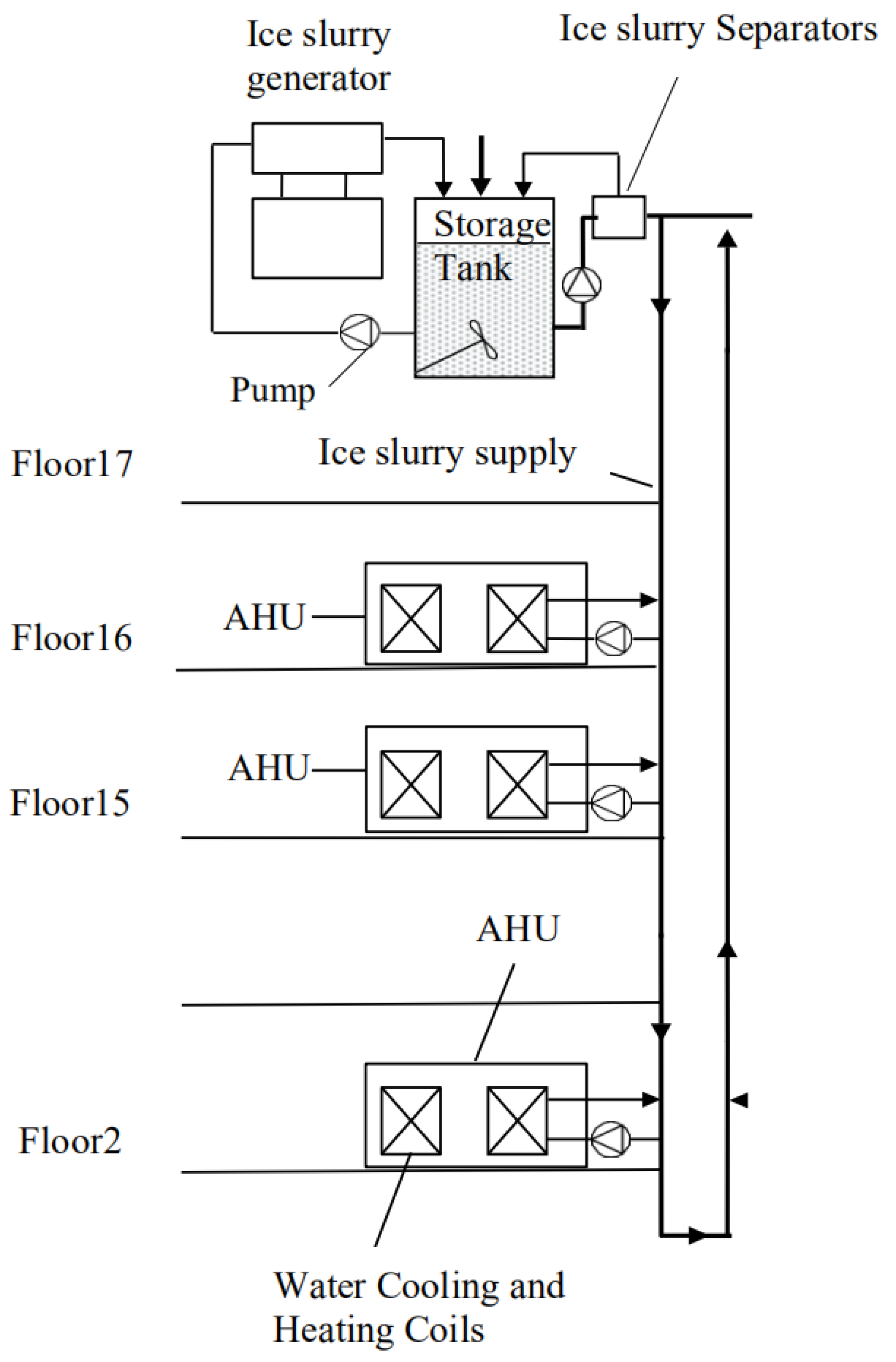
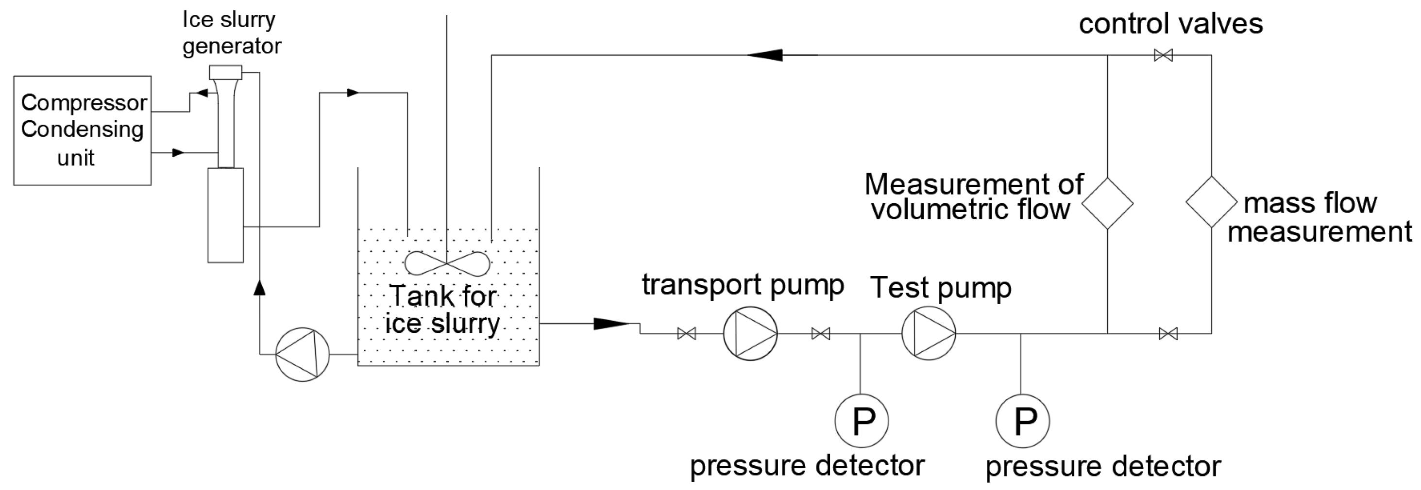
2.1. Ice Slurry Refrigeration System

The CAPCOM building [28] is located in the central district of Osaka, Japan, and is the R&D department of CAPCOM. It has 20 floors and a total floor area of 16,784 m2. The company’s offices are located on floors 2 to 16, each with an area of 570 m2. It has been calculated that the heat load in the office is 151 W/m2, which is relatively higher than that of the normal office building, due to the heat generated by the computers in the office. Thus, a gas-driven absorption refrigeration system was installed to provide cooling for the office area.
The cooling of the internal area of the office space of the building is provided by an ice slurry cooling system, as shown in Figure 1. The system consists of two ice slurry units, each with a cooling capacity of 272 kW. The ice slurry machine on the 17th floor produces ice stored in two tanks. The ice slurry from the storage tank is pumped to the air handling units on each floor through the ice slurry separator, which controls the ice mass fraction of the ice slurry up to 20%. Each of the 15 office floors has two air handling units with flow rates of 2.5 m3/s, which in turn provide six variable air volume (VAV) terminals. The low temperature of the ice slurry led to the choice of a cold air distribution temperature of 12 °C rather than 15 °C, which is a normal design practice in Japan. This reduced air flow requirements from 41 m3/h to 32 m3/h, resulting in smaller equipment sizes and lower power requirements for air distribution, and savings in capital and operating costs.
The working process of the ice slurry cooling system is shown in Figure 1 [29]. During the night time, the ice slurry was produced and stored in the tank as the electricity cost is relatively low during night time. In the daytime, owing to the increasing needs of the cooling demands, the ice slurry was pumped to the VAV terminals in each floor to compensate for the rising temperature in the offices. The ice slurry tank can be regarded as a cooling energy battery of the building. Thus, the energy cost and electricity bills are decreased by using this approach. Through the energy analysis of the system, the 16 layers that carry the ice slurry pipeline cost the main energy consumption. It is of great significance to study how to design the ice concentration and flow rate to reasonably reduce the pump power of the ice slurry system at different cooling capacity rates.

2.2. Simulation Models/Methods

According to their properties, fluids are usually classified as Newtonian or non-Newtonian. At present, the research on the flow characteristics of ice slurry, especially the non-Newtonian fluid characteristics, usually adopts two methods: fitting experimental data to obtain relevant empirical or semi-empirical formulae or using the existing non-Newtonian flow model to carry out theoretical calculation and analysis. Due to the limitation of experimental equipment, selection of working conditions, and slurry variability, the empirical or semi-empirical formulas obtained in the study have a certain applicable scope, and it is very difficult to determine the flow model of ice slurry accurately. Therefore, the work of this paper was not to study the pumping situation of ice slurry in the pipeline, but to determine the optimal concentration and flow of the pump inlet so that it can be transported to the pipeline through the internal pressure of the pump so as to reduce the consumption of pumping power and save energy.
The model of a single pump in the ice slurry system can be simplified as Figure 2, a simple ice slurry conveying pipeline composed of a storage tank, a transport pump, a test pump, and a control valve. The storage tank is the location of the ice slurry. The transport pump refers to all the pumps except the pump under study, and the test pump is the pump under study. The two flow meters and two pressure detectors in the figure are for data collecting. In this paper, the pumping model of ice slurry was studied by analyzing the experimental data of Nørgaard. The pump used in the experiment was a GrundfosCr2-50 centrifugal pump, in which the liquid solution was 16% propanediol, the diameter of the ice particles was between 0.1 mm and 0.3 mm, and the pump speed was 2800 r/min. Their experimental figure was selected as experimental data, and the data are shown in Table 1 and Table 2. According to the data in Table 1 and Table 2, MATLAB was used for data fitting, and the empirical formula related to ice concentration could be obtained by the pump efficiency calculation formula:
The ice concentration is defined by:
C = m i c e m
where:
C —the ice concentration in ice slurry (−),
m i c e —the mass of ice particles (kg),
m —the mass of ice slurry fluid (kg).
Pump efficiency calculation formula:
η = P e P × 100 %
where:
η —the pump efficiency (%),
P e —the pump power output (W),
P —the shaft power of the pump (W).
The pump power output can also be written as:
P e = ρ Q g H  
where:
P e —the pump power output (W),
ρ —the fluid density (kg/m3),
Q —the volume flow rate (m3/h),
g —the gravitational acceleration (m/s2),
H —the total head of the pump (m).
In ice slurry two-phase flow, the density of ice crystal and solution is different to some extent, and the density of ice slurry can be calculated by linear weighting of the two phase states:
ρ = 1 C ρ i + 1 C ρ S
where:
C —the ice concentration (−),
ρ —the fluid density (kg/m3),
ρ s —the density of the solution (kg/m3),
ρ i —the density of ice crystals (kg/m3),
According to the ASHRAE 2020 manual, the density of 16% propylene glycol solution is about 1020 kg/m3, and the density of ice is about 917 kg/m3.
Substituting Equation (3) into Equation (2), we can acquire [30]:
η = Q P · H · ρ · g
where:
η —the pump efficiency (%),
Q —the volume flow rate (m3/h),
P —the power consumption (i.e., the pump power) (W),
H —the total head of the pump (m),
ρ —the fluid density (kg/m3),
g —the gravitational acceleration (m/s2).
By using the curve fit tool of MATLAB to fit the data in Table 2, we can acquire Figure 3:
The R-square is 0.9117. R-square is generally used to evaluate the quality of the model in regression. The closer its value is to 1, the better the model performance is.
The fitting results are as follows:
H = 0.004873 Q 3 5.163 Q 2 C 22.33 C 2 Q 1267 C 3 2.025 Q 2 + 6.379 Q C + 527.1 C 2 0.378 Q 64.4 C + 45.74
where:
Q —the volume flow rate (m3/h),
H —the total head of the pump (m),
C —the ice concentration (−).
Such empirical formulas can only be applied in the range of 0% to 30% ice concentration.
By mathematically fitting the data of ice concentration and efficiency in Table 1 in the same way, we can acquire Figure 4 and Equation (7):
The R-square is 0.984. This shows that our model performs well.
η = 0.003569 Q 3 0.07549 Q 2 C 0.7032 C 2 Q 13.18 C 3 0.04356 Q 2 + 0.2108 Q C + 7.595 C 2 + 0.2584 Q 1.696 C + 0.1765
where:
Q —the volume flow rate (m3/h),
η —the pump efficiency (%),
C —the ice concentration (−).
Such an empirical formula of efficiency is applicable in a certain range and meaningless in another range. Meaningful ranges mainly include: the efficiency range being between 0 and 1, and therefore, the efficiency beyond this range is meaningless. Due to the performance of the pump, it does not make sense to exceed the flow rate and ice concentration that the pump can transport.
Substituting the above empirical head and efficiency Equations (5) and (6) into the theoretical pump efficiency Equation (4) mentioned above, the pump power can be obtained as follows:
P = ( 0.004873 Q 3 5.163 Q 2 C 22.33 C 2 Q 1267 C 3 2.025 Q 2 + 6.379 Q C + 527.1 C 2 0.378 Q 64.4 C + 45.74 ) / ( 0.003569 Q 3 0.07549 Q 2 C 0.7032 C 2 Q 13.18 C 3 0.04356 Q 2 + 0.2108 Q C + 7.595 C 2 + 0.2584 Q 1.696 C + 0.1765 ) 9.8 ρ Q / 3600
where:
Q —the volume flow rate (m3/h),
ρ —the fluid density (kg/m3),
C —the ice concentration (−).
We use (μ,λ) evolutionary strategy algorithm [31] for optimization. Here are the main steps of the algorithm [32]:
First, the problem to be solved by the algorithm must be determined. The problem of solving the optimal concentration into a mathematical problem should be transformed: solving the minimum value of Equation (7). The algorithm flow chart is shown in Figure 5.
Set up an initial population, which is the first generation of parents for evolution (which can be randomly generated). The parent should be a matrix composed of concentration and flow, the first behavior is concentration, and the second behavior is flow, one of which represents a set of solutions to the function P. Considering the running time and the accuracy of the results, the initial population size as 10 was set. That is, there are 10 solutions of P functions in the initial population matrix.
Next, the evolution of the population should be started [33]. Step one, cross out parents. For example, two groups of random solutions (concentration 0.1 flow 2) and (concentration 0.2 flow 1) in the parent, then the concentration or flow of the two groups of solutions needed to be interchanged, which becomes (concentration 0.1 flow 1) and (concentration 0.2 flow 2). This is to make the range of data solution more extensive, to avoid only small concentration against small flow, large concentration against large flow situations. Step two, the program has to start mutating, which is basically adding a variable to each of the two quantities of each set of solutions. This variable satisfies a Gaussian distribution of some zero mean and some variance. The variance is called the degree of variation in the evolutionary strategy algorithm. So, if you add this variable, you are adding a degree of variation to each of the solutions, which is an indication of how much the solutions have changed. When the population evolves to convergence, the degree of variation will also gradually decrease, making the whole population converge easier. In general, crossover and variation are designed to make the values of concentration and flow more “random” within the allowable range. In this way, the group of solutions which makes the pump power minimum has a higher probability of appearing.
The data completed by mutation, namely, the offspring, were selected. Generally speaking, the ratio of parents to offspring in (μ, λ) selection strategy was 1:7 [34]. Since the parent was set as 10 above, the offspring should be 70. The pump power matrix corresponding to the subgeneration solution can be obtained by calculating 70 subgenerations into the pump power formula. The pump power matrices of 70 groups of solutions were compared, and the 10 groups with the least pump power were finally selected. These 10 groups of solutions were taken as new parents, namely the second generation parents, so as to carry out the next evolution. Eventually, generation after generation, the population must converge to the optimal solution we need.
Essentially, this is an evolutionary strategy algorithm, a probabilistic algorithm that takes a random value and then calculates a comparative fitness [35]. The advantage of this algorithm is that the optimal concentration of ice slurry is a practical problem, and its mathematical model is necessarily very complicated, which is difficult to analyze by ordinary methods. By using the evolutionary strategy algorithm, the function properties can be ignored, the optimal value can be obtained easily [36], and the problem of local optimization can be avoided. However, with the increase of iteration times, the optimal value becomes more accurate, but the running time is also greatly increased.

3. Results

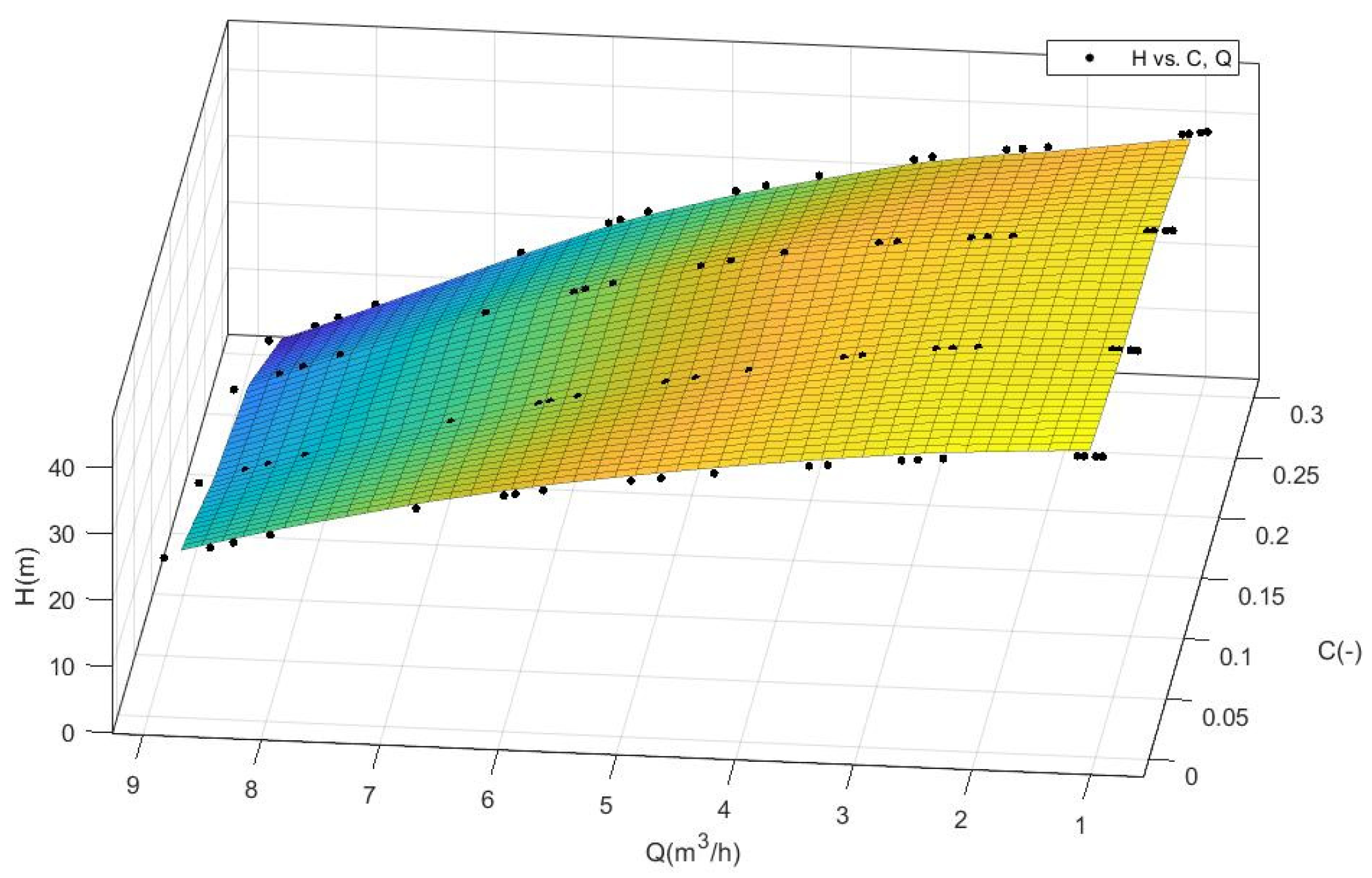
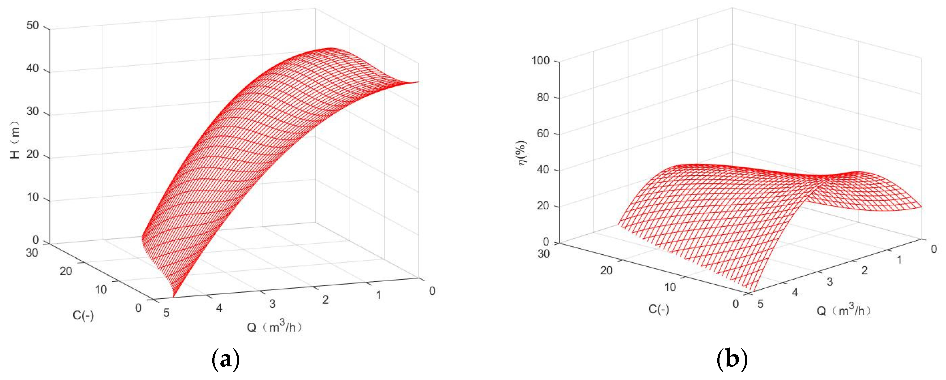
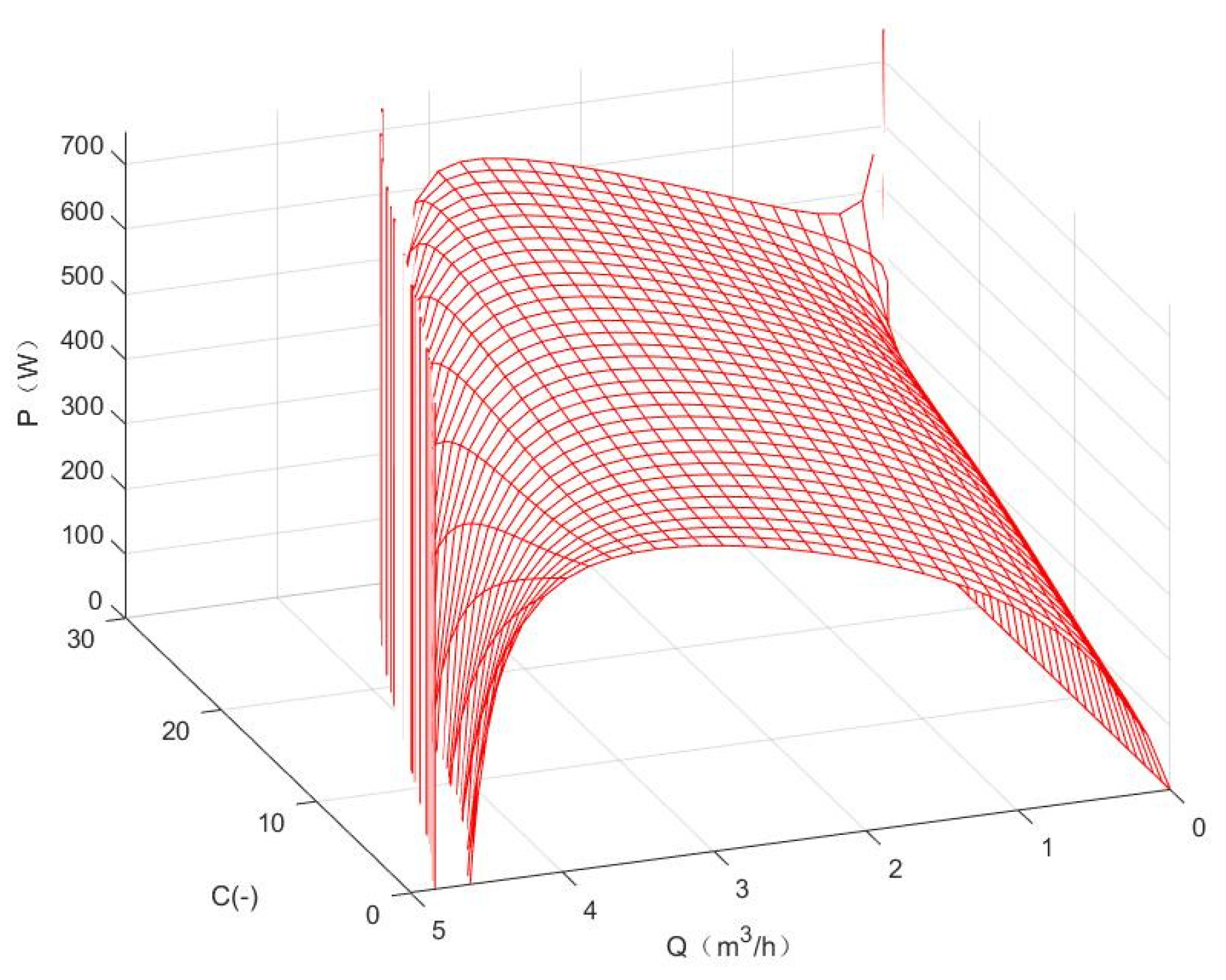
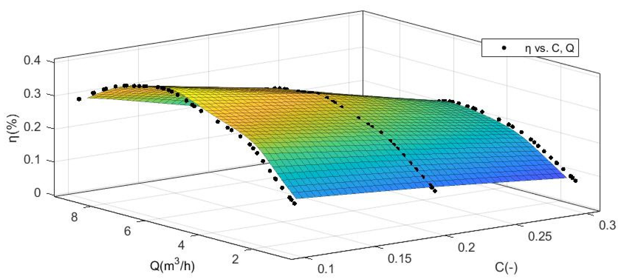
3.1. Empirical Function Diagram

MATLAB was used to draw Equations (6) and (7). The drawing range is 0~30% of ice concentration and 0~5 m3/h of flow, and Figure 6a,b can be obtained:
As can be seen from Figure 6a, when the concentration increased, the head of the pump did not change much at the same flow rate, but the flow that the pump can transport was even smaller. When the ice concentration reached the system limit of 30%, the pump flow was only about 0.5 m3/h. The reason for this situation is that the power of the pump has a limit. Under the condition of a certain speed, with the increase of concentration, the energy consumption of conveying ice slurry per unit flow rate is higher. In order to make the ice slurry reach the required head, only a small part of the ice slurry can be transported at the expense of the flow. It also shows that the properties of ice slurry are different from an ordinary water solution. Obviously, the energy consumption of conveying water is much lower than that of conveying ice slurry. Due to the Q-H characteristics of the pump itself, the flow rate must decrease with the rise of the head, but at high ice concentrations, the flow rate decreases more rapidly. Thus, in general, as the concentration increases, the pump can deliver less flow.
As can be seen from Figure 6b, when the concentration increased, the efficiency of the pump decreased continuously. That is to say, the higher the concentration, the more difficult the pump is to pump, which is consistent with the pump characteristics and the rise of the flow, so that the pump efficiency rose to the maximum value and then decreased. The flow rose to the level that pump can withstand the extreme value; at this time the pump power is infinite and meaningless, and the efficiency is zero.
According to the analysis of the above two figures, it is consistent with the influence of two-phase flow on the pump: when the concentration of conveying ice particles increased, the head decreased less at a small flow rate, but the drop was larger at a large flow rate. As the concentration increased, the maximum flow rate of the pump gradually decreased, and in order to achieve the required head, the power will increase and the efficiency will decrease. This also shows that such an empirical formula is valid in a certain range, and this analysis method has a certain practical significance.
Then, the pump power was analyzed in the same way, and Equation (8) was plotted using MATLAB. The drawing range was 0~30% ice concentration, 0~5 m3/h flow, and 0~750 W pump power, and Figure 7 could be obtained.
There are abnormal data in the upper left corner of Figure 7. This is because our models are based on experimental practice and only consider their mathematical characteristics. In fact, when the ice slurry transportation rate exceeds the pump’s capacity to transport the limit, the pump cannot work, which is shown in the mathematical model that the pump power is infinite. Obviously, too much flow and ice concentration can cause infinite pump power.

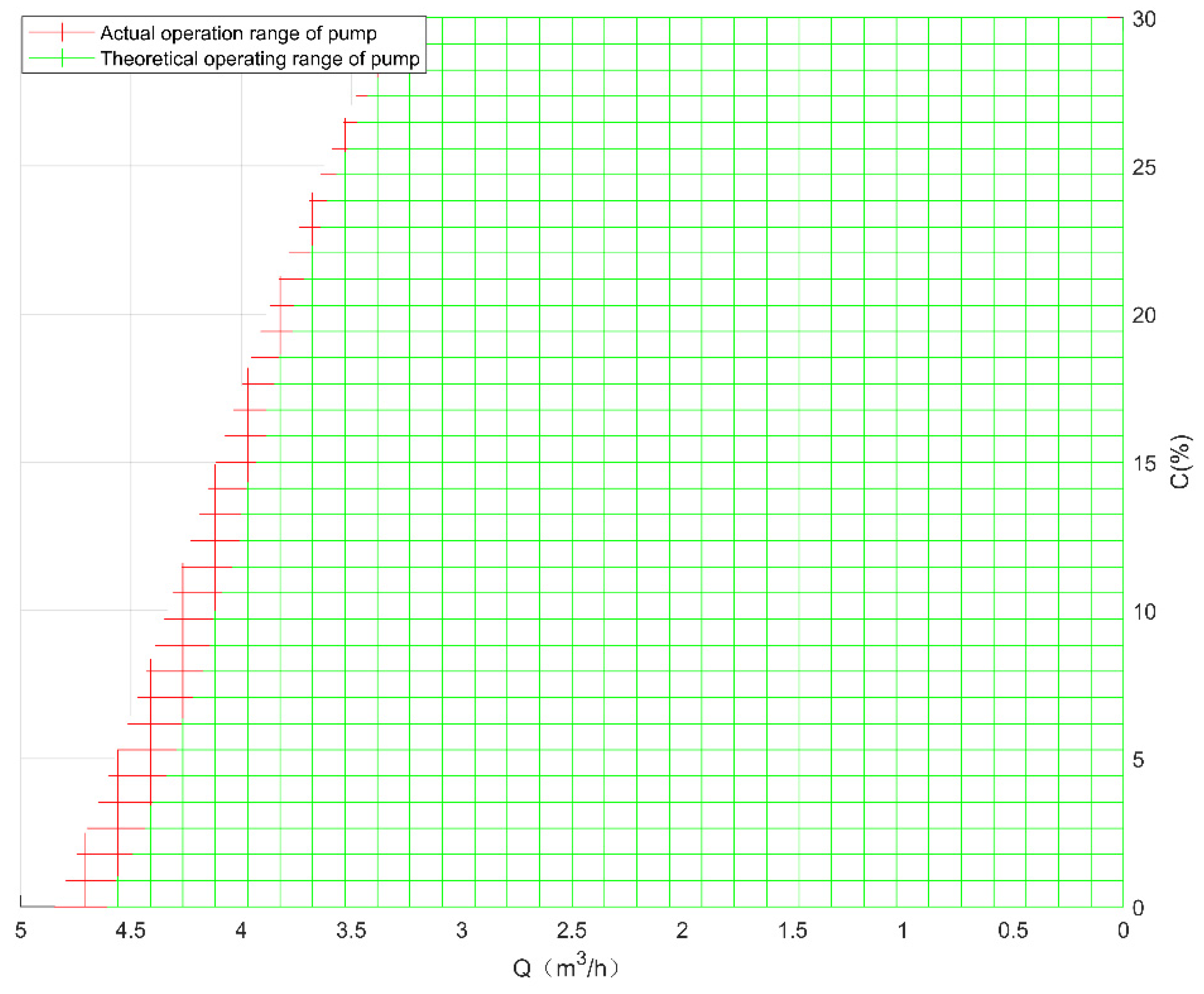
3.2. The Operation Range of Pump

Combining with the influence of flow rate and ice concentration, the flow rate of high ice concentration ice slurry transported by this system should not exceed 3.5 m3/h. The operating range of the pump is approximately shown in Figure 8.
The actual operating range of the pump is larger than the theoretical operation, and the actual range of the flow is larger. The reason is that, at a certain flow rate and at the ice concentration (where the flow does not exceed the maximum capacity of the pump), the pump efficiency is not zero (the pump is still running at rated power or over-rated power), but the it is already very small, and the pump power required to reach the pump required flow, although not infinite, exceeds the pump’s limit power, in which case the pump is prone to blockage, damage, and system failure. Therefore, in the design of the algorithm, we avoided this situation, so in theory, the flow rate of the pump runs in a smaller range [37].

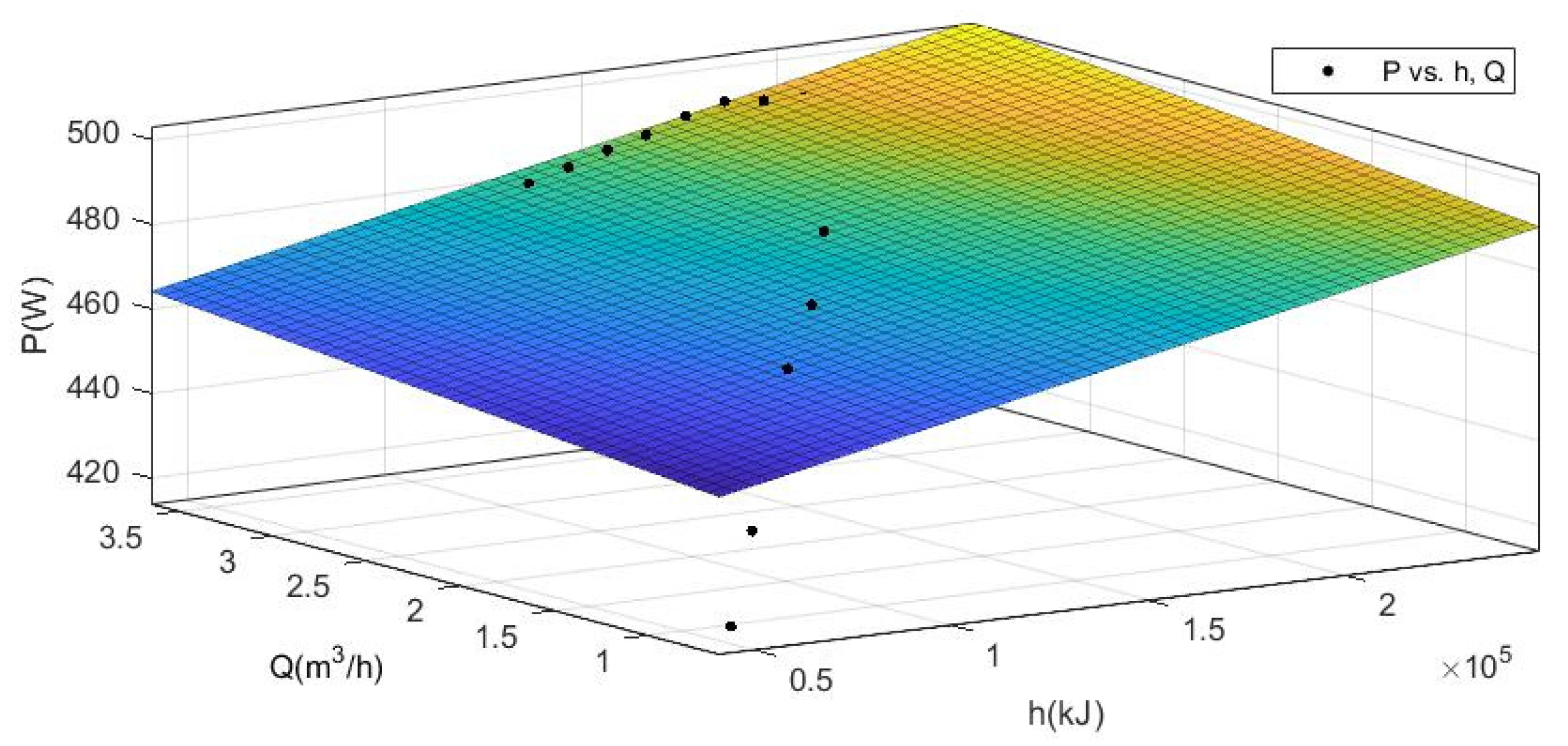
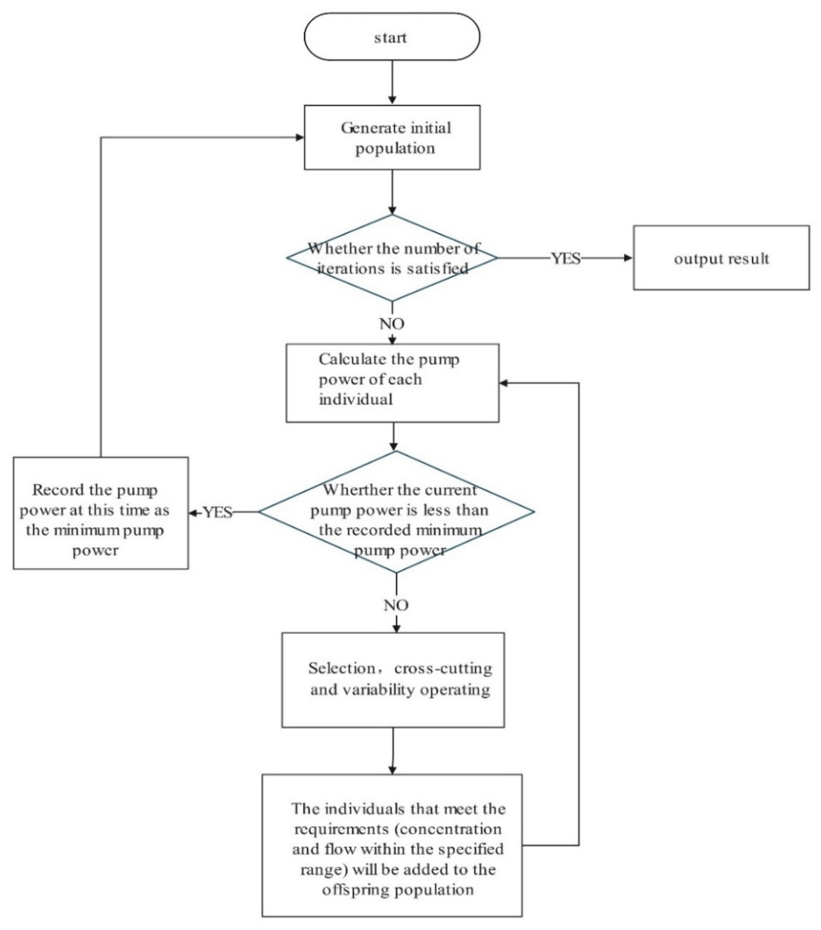
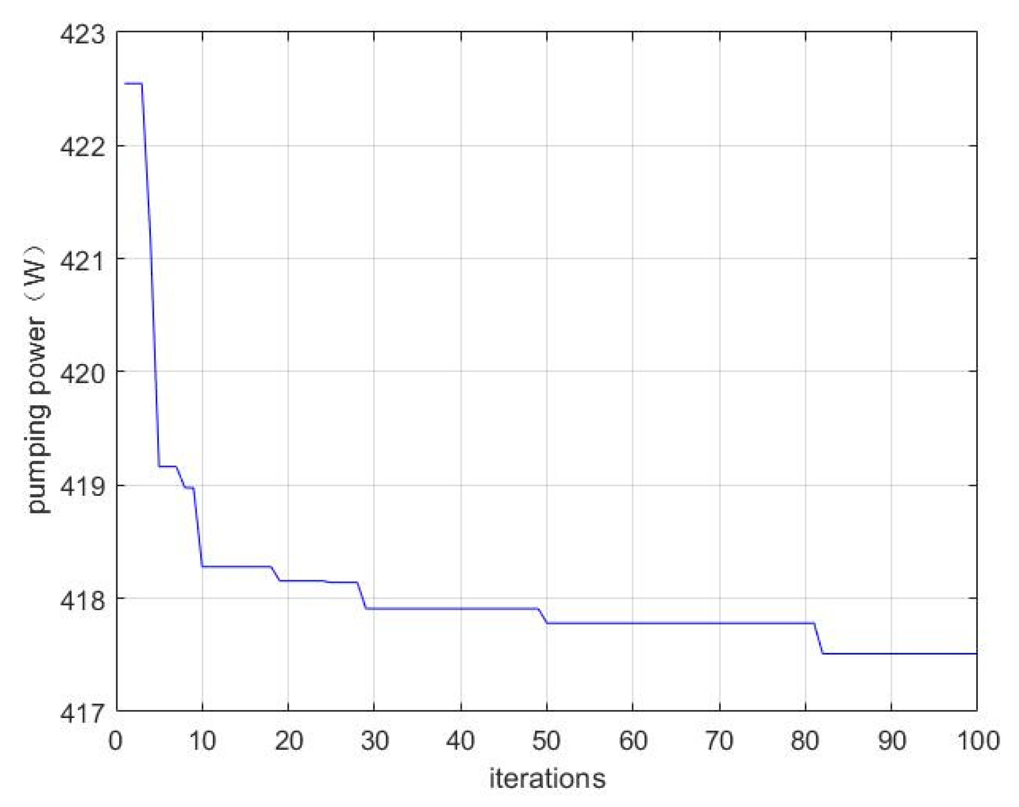
3.3. Apply the Optimal Algorithm

To apply the optimal concentration algorithm, first we should define what is “optimal”, which will be the key to the whole algorithm. The criterion of “optimal” was treated as the fitness in the evolutionary strategy algorithm. The process of finding the best fitness by the algorithm is the process of optimizing the concentration.
From the engineering practice, the optimal concentration is the concentration with the highest economic benefit. Therefore, it is defined that the concentration that minimizes the work of the conveying pump is the optimal concentration under the condition of satisfying an equal cooling capacity. In the algorithm, the pump power is the fitness. The smaller the pump power is, the better the fitness is.
The cooling capacity [38] of energy is set to meet the requirements. According to the energy absorbed by ice melting phase change and the conservation law of heat transfer, the following equation can be obtained:
h = Q ρ t h l s C
where:
h —the enthalpy change (J),
Q —the volume flow rate (m3/h),
ρ —the fluid density (kg/m3),
t —the time (s),
h l s —the latent heat of ice (kJ /kg),
C —the ice concentration (−).
The greater the change in enthalpy, the more energy is absorbed during the phase transition. Therefore, the larger is, the better its cold storage performance is. That is, when:
h < = 335 Q C ρ t
where:
h —the enthalpy change (J),
Q —the volume flow rate (m3/h),
ρ —the fluid density (kg/m3),
t —the time (s).
C —the ice concentration (−).
That is, it can be judged to satisfy the supply demand. This expression can be used as a selection condition of the algorithm. The optimal concentration was obtained by using the algorithm.
Taking h = 13.889 kWh (50,000 kJ) and the maximum operating power of the pump as 750 W, we can obtain Figure 9 and C = 0.1968 (the ice concentration) and Q   = 0.7587 (the volume flow rate).
Algorithm running results shows that when the required supply h = 13.889 kWh is met, the ice concentration is 19.68% and the volume flow rate is 0.7587 m3/h, that is, 2.1075 × 10⁻⁴ m3/s, making the pump power a minimum of 417.7 W.

3.4. Comparison under Different Cooling Capacity

Adjust the cooling capacity and put it into the algorithm. After multiple calculations, the data shown in Table 3 were obtained.
It can be found from Table 3 that the optimal concentration is stable at about 20% with little change, indicating that the optimal concentration does not change with the cooling capacity, while the optimal flow rate changes greatly. For that, we take concentration for a constant 20%, will be cooling capacity and flow rate, pump power, and data fitting, and acquiring the graphics as shown in Figure 10; as can be seen, the relationship is linear, and with the rise of the cooling capacity, the best flow and pump power will rise to meet the needs of cooling capacity, but after the flow rapidly rises, it reached the peak. Pump power is slowly rising due to the limitation of its own pump power, but also slowly reaches the peak, no longer rising.
It should be noted that there is a limit to the cooling capacity h that the system can supply for a period of time due to the upper limit of pump power. When applying the algorithm, be careful not to set the h value of cooling capacity beyond the limit, otherwise there will be operational error.

4. Conclusions

In this paper, a single pump in the ice slurry system was taken as the research object, and a set of optimal fluid pumping layout schemes were given by using the evolutionary strategy algorithm through the constructed pumping model. When the rated speed of Grundfos CR2-50 centrifugal pump or other centrifugal pumps with similar performance was 2800 r/min, to meet the cooling capacity of 13.889 kWh, the ice concentration at 19.68% and the ice slurry fluid flow of 2.1075 × 10⁻⁴ m3/s could minimize the pump operation and save transportation cost. In order to facilitate comparison, when the required cooling capacity was constant, the required concentration and flow were calculated by the algorithm. Only 417.7 W power is needed to meet the requirements. The calculation showed a 23% reduction in power consumption. In addition, the optimum concentration, flow rate, and pump power under different cooling capacities were analyzed, and the linear relationship was obtained. The ideas provided in this paper for the construction of ice slurry system are as follows: When the cooling demand needs to be calculated, we can optimize it from the algorithm level to get the best flow, concentration, and power so as to save energy and avoid wasting resources.

Author Contributions

Data curation, S.H.; Formal analysis, W.Z., S.H.; Funding acquisition, W.Z. and J.W.; Investigation, J.L.; Writing—original draft, S.H.; Writing—review & editing, S.H. and W.Z. All authors have read and agreed to the published version of the manuscript.

Funding

This research is sponsored by the Zhejiang Provincial Natural Science Foundation of China grant number LY21E060003 and Key Research and Development Plan of Zhejiang Province of China under Grant 2021C03034.

Institutional Review Board Statement

Not applicable.

Informed Consent Statement

Not applicable.

Data Availability Statement

Not applicable.

Acknowledgments

The author thanks the anonymous reviewers for their constructive comments and the editor for handling the paper.

Conflicts of Interest

The authors declare no conflict of interest.

References

  1. Illán, F.; Viedma, A. Heat exchanger performance modeling using ice slurry as secondary refrigerant. Int. J. Refrig. 2012, 35, 1275–1283. [Google Scholar] [CrossRef]
  2. Sosa, J.E.; Ribeiro, R.P.P.L.; Castro, P.J.; Mota, J.P.B.; Araújo, J.M.M.; Pereiro, A.B. Absorption of Fluorinated Greenhouse Gases Using Fluorinated Ionic Liquids. Ind. Eng. Chem. Res. 2019, 58, 20769–20778. [Google Scholar] [CrossRef]
  3. Purohit, P.; Oglund-Isaksson, L.H. Global emissions of fluorinated greenhouse gases 2005–2050 with abatement potentials and costs. Atmos. Chem. Phys. 2017, 17, 2795–2816. [Google Scholar] [CrossRef] [Green Version]
  4. Sosa, J.E.; Malheiro, C.; Ribeiro, R.P.; Castro, P.J.; Piñeiro, M.M.; Araújo, J.M.; Plantier, F.; Mota, J.P.; Pereiro, A.B. Adsorption of fluorinated greenhouse gases on activated carbons: Evaluation of their potential for gas separation. J. Chem. Technol. Biotechnol. 2020, 95, 1892–1905. [Google Scholar] [CrossRef]
  5. Bellas, I.; Tassou, S.A. Present and future applications of ice slurries. Int. J. Refrig. 2005, 28, 115–121. [Google Scholar] [CrossRef]
  6. Kumano, H.; Hirata, T.; Shirakawa, M.; Shouji, R.; Hagiwara, Y. Flow characteristics of ice slurry in narrow tubes. Int. J. Refrig. 2010, 33, 1513–1522. [Google Scholar] [CrossRef]
  7. Kauffeld, M.; Wang, M.J.; Goldstein, V.; Kasza, K.E. Ice slurry applications. Int. J. Refrig. 2010, 33, 1491–1505. [Google Scholar] [CrossRef] [Green Version]
  8. Vetterli, J.; Benz, M. Cost-optimal design of an ice-storage cooling system using mixed-integer linear programming techniques under various electricity tariff schemes. Energy Build. 2012, 49, 226–234. [Google Scholar] [CrossRef]
  9. Henze, G.P.; Krarti, M.; Brandemuehl, M.J. Guidelines for improved performance of ice storage systems. Energy Build. 2003, 35, 111–127. [Google Scholar] [CrossRef]
  10. Lee, W.; Chen, Y.T.; Wu, T. Optimization for ice-storage air-conditioning system using particle swarm algorithm. Appl. Energy 2009, 86, 1589–1595. [Google Scholar] [CrossRef]
  11. Ise, H.; Tanino, M.; Kozawa, Y. Ice Storage System in Kyoto Station Building. In Proceedings of the Information Booklet for the Technical Tour of the Fourth IIR Workshop on Ice Slurries, Kyoto, Japan, 13 November 2001; pp. 11–16. [Google Scholar]
  12. Kousksou, T.; Arid, A.; Majid, J.; Zeraouli, Y. Numerical modeling of double-diffusive convection in ice slurry storage tank. Int. J. Refrig. 2010, 33, 1550–1558. [Google Scholar] [CrossRef]
  13. Frei, B.; Huber, H. Characteristics of different pump types operating with ice slurry. Int. J. Refrig. 2005, 28, 92–97. [Google Scholar] [CrossRef]
  14. Nørgaard, E.; Sørensen, T.A.; Hansen, T.M.; Kauffeld, M. Performance of components of ice slurry systems: Pumps, plate heat exchangers, and fittings. Int. J. Refrig. 2005, 28, 83–91. [Google Scholar] [CrossRef]
  15. Kumano, H.; Hirata, T.; Shouji, R.; Shirakawa, M. Experimental study on heat transfer characteristics of ice slurry. Int. J. Refrig. 2010, 33, 1540–1549. [Google Scholar] [CrossRef]
  16. Žurovec, D.; Jezerská, L.; Nečas, J.; Hlosta, J.; Diviš, J.; Zegzulka, J. Spiral Vibration Cooler for Continual Cooling of Biomass Pellets. Processes 2021, 9, 1060. [Google Scholar] [CrossRef]
  17. Almeida, R.H.; Ledesma, J.R.; Carrêlo, I.B.; Narvarte, L.; Ferrara, G.; Antipodi, L. A new pump selection method for large-power PV irrigation systems at a variable frequency. Energy Convers. Manag. 2018, 174, 874–885. [Google Scholar] [CrossRef] [Green Version]
  18. Wu, Z.; Sha, L.; Yang, X.; Zhang, Y. Performance evaluation and working fluid selection of combined heat pump and power generation system (HP-PGs) using multi-objective optimization. Energy Convers. Manag. 2020, 221, 113164. [Google Scholar] [CrossRef]
  19. Zhang, J.; Chao, Q.; Xu, B. Analysis of the cylinder block tilting inertia moment and its effect on the performance of high-speed electro-hydrostatic actuator pumps of aircraft. Chin. J. Aeronaut. 2018, 31, 169–177. [Google Scholar] [CrossRef]
  20. Warguła, A.; Kukla, M. Determination of maximum torque during carpentry waste comminution. Wood Res.-Slovak. 2020, 65, 771–784. [Google Scholar] [CrossRef]
  21. Yoon, H.; Lee, J.; Kim, M.; Kim, E.; Shin, Y.; Kim, S.; Min, S.; Ahn, S. Power Consumption Assessment of Machine Tool Feed Drive Units. Int. J. Precis. Eng. Manuf. Technol. 2020, 7, 455–464. [Google Scholar] [CrossRef]
  22. Van Nang, N.; Matsuo, T.; Koumoto, T.; Inaba, S. Measurement of the properties of agricultural tire for tractor dynamic analyses (Part 1)-Determination of drive tire stiffness and damping from static tests. J. Jpn. Soc. Agric. Mach. 2009, 71, 55–62. [Google Scholar]
  23. Klarecki, K.; Rabsztyn, D.; Hetmańczyk, M.P. Influence of the Controller Settings on the Behaviour of the Hydraulic Servo Drive; Awrejcewicz, J., Szewczyk, R., Trojnacki, M., Kaliczyńska, M., Eds.; Springer International Publishing: Cham, Switzerland, 2015; pp. 91–100. [Google Scholar]
  24. Warguła, A.; Kukla, M.; Krawiec, P.; Wieczorek, B. Impact of Number of Operators and Distance to Branch Piles on Woodchipper Operation. Forests 2020, 11, 598. [Google Scholar] [CrossRef]
  25. Paryanto; Brossog, M.; Bornschlegl, M.; Franke, J. Reducing the energy consumption of industrial robots in manufacturing systems. Int. J. Adv. Manuf. Technol. 2015, 78, 1315–1328. [Google Scholar] [CrossRef]
  26. Kuchmacz, J.; Niezgoda-Żelasko, B. Ice slurry flow through a vertical slit channel. Int. J. Refrig. 2021, 128, 34–42. [Google Scholar] [CrossRef]
  27. Morimoto, T.; Komatsu, W.; Kimata, H.; Kato, M.; Kumano, H. Solidification behavior of an ice slurry flowing in a rectangular channel. Int. J. Refrig. 2021. [Google Scholar] [CrossRef]
  28. Kauffeld, M.; Kawaji, M.; Egolf, P.W. Handbook_on_ice_slurries. Int. J. Refrig. 2005, 3, 415–427. [Google Scholar]
  29. Davies, T.W. Slurry ice as a heat transfer fluid with a large number of application domains. Int. J. Refrig. 2005, 28, 108–114. [Google Scholar] [CrossRef]
  30. Kitanovski, A.; Vuarnoz, D.; Ata-Caesar, D.; Egolf, P.W.; Hansen, T.M.; Doetsch, C. The fluid dynamics of ice slurry. Int. J. Refrig. 2005, 28, 37–50. [Google Scholar] [CrossRef]
  31. Zhang, W.; Lin, L.; Gen, M.; Chien, C. Hybrid Sampling Strategy-based Multiobjective Evolutionary Algorithm. Procedia Comput. Sci. 2012, 12, 96–101. [Google Scholar] [CrossRef] [Green Version]
  32. Wu, G.; Pedrycz, W.; Suganthan, P.N.; Mallipeddi, R. A variable reduction strategy for evolutionary algorithms handling equality constraints. Appl. Soft Comput. 2015, 37, 774–786. [Google Scholar] [CrossRef]
  33. Arruda, E.F.; Kagan, N.; Ribeiro, P.F. Three-phase harmonic distortion state estimation algorithm based on evolutionary strategies. Electr. Power Syst. Res. 2010, 80, 1024–1032. [Google Scholar] [CrossRef]
  34. Liang, Z.; Hou, W.; Huang, X.; Zhu, Z. Two new reference vector adaptation strategies for many-objective evolutionary algorithms. Inf. Sci. 2019, 483, 332–349. [Google Scholar] [CrossRef]
  35. Ma, T.; Yan, Q.; Tian, W.; Guan, D.; Lee, S. Replica creation strategy based on quantum evolutionary algorithm in data gird. Knowl.-Based Syst. 2013, 42, 85–96. [Google Scholar] [CrossRef]
  36. Li, L.; Lin, W.; Lin, Q.; Ming, Z. Balancing Convergence and Diversity in Multiobjective Immune Algorithm. In Proceedings of the 2020 12th International Conference on Advanced Computational Intelligence (ICACI), Dali, China, 14–16 August 2020; pp. 102–109. [Google Scholar]
  37. Jin, N.; Tsang, E. Bargaining strategies designed by evolutionary algorithms. Appl. Soft Comput. 2011, 11, 4701–4712. [Google Scholar] [CrossRef]
  38. Jeong, E.S. Optimization of thermoelectric modules for maximum cooling capacity. Cryogenics 2021, 114, 103241. [Google Scholar] [CrossRef]
Figure 1. Schematic diagram of the ice slurry cooling system in the CAPCOM building.
Energies 14 06738 g001
Figure 2. The ice slurry pumping model of a single pump.
Energies 14 06738 g002
Figure 3. Fitting graph of pump Q-H data.
Energies 14 06738 g003
Figure 4. Fitting graph of pump efficiency data.
Energies 14 06738 g004
Figure 5. Algorithm flow chart.
Energies 14 06738 g005
Figure 6. (a) Empirical function diagram of ice concentration and head and (b) ice concentration and pump efficiency.
Energies 14 06738 g006
Figure 7. Empirical function diagram of ice concentration and pump power.
Energies 14 06738 g007
Figure 8. Operation range of pump.
Energies 14 06738 g008
Figure 9. Running results of optimal ice concentration algorithm.
Energies 14 06738 g009
Figure 10. Variation of the optimal flow rate and pump power as the cooling capacity changes.
Energies 14 06738 g010
Table 1. Pump efficiency Q-η data at different ice concentrations.
Q η
(C = 0%)
η
(C = 10%)
η
(C = 20%)
η
(C = 30%)
×10−4 (m3/s)%%%%
0.933 17.832 14.991 12.151 8.581
1.043 19.777 15.882 12.928 9.182
1.098 20.715 16.324 13.316 9.483
1.116 21.022 16.471 13.446 9.583
1.391 25.338 18.725 15.386 11.084
1.629 28.636 20.821 17.062 12.381
1.647 28.903 20.988 17.190 12.481
1.848 32.093 22.861 18.597 13.571
2.104 35.093 25.246 20.366 14.946
2.324 36.718 27.193 21.849 16.103
2.470 37.715 28.361 22.808 16.853
2.598 38.627 29.240 23.614 17.477
2.946 40.710 30.935 25.387 18.889
3.276 42.162 32.063 26.370 19.836
3.422 42.737 32.508 26.787 20.179
3.788 44.070 33.544 27.907 20.915
4.410 46.024 35.407 29.855 21.878
4.666 46.678 36.316 30.629 22.170
4.739 46.849 36.578 30.843 22.240
4.959 47.334 37.346 31.445 22.407
5.288 48.030 38.391 32.026 22.511
5.508 48.535 38.920 31.804 22.454
5.618 48.896 39.097 31.615 22.373
5.801 49.279 39.226 31.406 22.130
5.856 49.316 39.224 31.357 22.022
6.020 49.387 39.123 31.227 21.547
6.459 49.388 38.440 30.904 19.186
6.533 49.362 38.300 30.838 18.774
6.716 49.254 37.943 30.618 17.795
6.899 49.069 37.595 30.252 16.857
7.191 48.607 37.044 29.317 15.393
7.265 48.463 36.881 29.048 15.029
7.594 47.727 35.925 27.773 13.280
7.960 46.862 34.453 26.241 10.687
7.978 46.818 34.371 26.160 10.537
8.033 46.688 34.118 25.910 10.080
8.399 45.825 32.301 23.738 6.817
8.436 45.740 32.109 23.456 6.478
8.948 44.348 29.261 19.119 1.624
8.96644.285 29.153 18.943 1.449
Table 2. Q-H data at different ice concentrations.
QH
(C = 0%)
H
(C = 10%)
H
(C = 20%)
H
(C = 30%)
×10−4 (m3/s)(m)(m)(m)(m)
0.938 45.336 43.123 43.024 39.705
0.996 45.311 43.113 42.942 39.552
1.094 45.268 43.097 42.806 39.298
1.152 45.239 43.087 42.724 39.146
2.285 44.004 42.499 41.103 36.381
2.500 43.657 42.208 40.776 35.960
2.637 43.425 41.978 40.561 35.704
3.262 42.274 40.501 39.485 34.142
3.418 41.966 40.050 39.179 33.615
4.219 40.264 37.500 37.132 30.550
4.668 39.213 36.037 35.529 28.731
4.922 38.584 35.189 34.515 27.696
5.664 36.567 32.477 31.333 24.050
5.898 35.862 31.530 30.265 22.634
5.996 35.558 31.122 29.810 22.015
6.738 33.037 27.828 26.119 16.992
7.969 28.075 21.828 18.798 8.209
8.281 26.679 20.206 16.766 5.994
8.477 25.786 19.167 15.485 4.639
8.867 23.939 17.024 12.915 2.052
Table 3. C, Q, and P data of different h.
h
(kJ)
C
(−)
Q
(m3/h)
P
(W)
50,0000.20190.742417.7741
60,0000.21450.838438.0961
70,0000.22590.9281455.7548
80,0000.22441.068471.3064
90,0000.23241.1488484.3047
100,0000.23211.2917498.7775
110,0000.20453.4994475.4409
120,0000.23573.499477.3328
130,0000.20143.4985480.6834
140,0000.22193.4963483.3599
150,0000.20563.4978486.1921
160,0000.21363.4999488.5491
170,0000.21453.4994491.9074
180,0000.20963.4987494.1524
190,0000.21013.4998493.1199
200,0000.21213.4978492.5956
210,0000.21253.4984491.9436
220,0000.21183.4996491.8095
230,0000.21223.4995491.532
240,0000.21153.4993492.2494
Publisher’s Note: MDPI stays neutral with regard to jurisdictional claims in published maps and institutional affiliations.

