1. Introduction
A significant amount of greenhouse gas emissions are produced by the transportation sector. Particularly, internal-combustion-engine-powered heavy-duty vehicles (HDVs) fuelled with diesel are one of the highest energy-intensive freight modes and major greenhouse gas emitters. HDVs produce approximately 16% of the CO
2 worldwide [
1], and 20% of the transportation sector greenhouse emissions [
2] in the United States. HDVs are separated in the United States into classes defined by weight limits, where higher class numbers indicate a greater weight limit: Class 2b includes vans and heavy-duty pickup trucks, Classes 3–5 include city delivery trucks, Class 7 includes city buses, and Class 8 includes long-haul trucks and coach buses [
3] (similar to classes N and O in Europe). The global emissions from Class 8 heavy-duty long-haul trucks (Europe Class O4) will more than double in the near future in the absence of mitigating emission policies due to the continuing and strong growth of the on-road transportation sector, especially in developing countries [
4]. Policies and actions to mitigate harmful emissions from transportation include vehicle powertrain hybridization and electrification, reductions in carbon intensity of fuel, freight modal shifts, design for demand, and overall vehicle efficiency improvements. Many studies have shown the feasibility of increasing the fuel economy of HDVs up to 30% by using a variety of drive train technologies as summarized in [
4]. The impact of drive train technologies and fuel savings depends on the vehicle operation conditions, i.e., whether the vehicle is used for long haul shipments, highly characterized by long steady-state motion periods, or urban traffic, characterized by transient stop-and-go operation [
4].
The emission and fuel consumption reduction task is considered difficult due to the diversity and magnitude of the road transportation sector conditions in different countries [
4]. Lately, particular attention has been focused on the design, realization, and optimal operation of fully electric or hybrid vehicles [
5]. Specifically, an online optimal control strategy for a hybrid power split electric bus based on historical data was proposed in [
6]. Their goal is to fully exploit the fuel saving capability of a power split hybrid electric bus under a real-time operating cycle to achieve an effective strategy for solving the optimal calibration problem online. First, they constructed a procedure for synthesizing a real-time driving cycle based on the Markov method and clustered analysis. Second, an optimal controller based on dynamic programming (DP) was developed to investigate fuel economy potential. A rule control method was used as the basis for an online approximation of the DP controller, since DP is not practical for real-time applications. Lastly, a hardware in-the-loop test and offline simulation were conducted. Results showed that the proposed online control gives approximately similar fuel consumption minimization compared to the DP optimal control and achieves real-world improvements.
Lombardi et al. [
7] tested six heavy-duty Class 8 truck powertrain configurations: a conventional diesel engine, a diesel engine modified to operate on an organic Rankine cycle (ORC), a diesel-engine-based series hybrid system, an ORC diesel-based series hybrid system, a diesel-engine-based parallel hybrid system, and an ORC diesel-based parallel hybrid system. An optimal control strategy derived from Pontryagin’s Minimum Principle was used to minimize the total fuel consumption of the vehicle during the driving cycle and to provide power thresholds needed for a rule-based energy management control strategy. Simulations showed that the parallel hybrids result in the most fuel saving and CO
2 reduction.
Energy management control strategy of a hydraulic electric hybrid medium duty vehicle was investigated in [
8]. Mathematical models of a pure electric vehicle and a hydraulic electric hybrid vehicle were developed to model the variations of battery charging states and torque through the United States Environmental Protection Agency’s New York City Cycle. A rule-based energy management control was proposed. Adjustment of the rule control strategy was performed using a genetic algorithm to refine the vehicle electricity economic performance. Results show that the designed hydraulic hybrid vehicle electricity performance was improved by 36.5% compared to that of a pure electric vehicle. The energy consumption performance was improved by 43.7% after applying the genetic algorithm refined strategy.
A nonlinear model predictive control (NMPC) for heavy-duty hybrid electric vehicles using a random power prediction method was proposed in [
9]. They combined Markov chains and grey models to produce high-accuracy, ultra-short-term power prediction to account for the lack of navigation information. The predicted power is incorporated into a multi-objective NMPC optimization of bus voltage, a battery state of charge, and fuel consumption. The NMPC was validated in a hardware-in-the-loop simulation platform and compared against other control approaches: rule-based control, fuzzy logic, and dynamic programming. Results showed that the proposed control strategy gives a better all around performance compared to the rule-based and fuzzy approaches. However, the fuel consumption obtained by the online NMPC was approximately 7.7% more than that achieved by the offline dynamic programming global optimization strategy.
Zhang et al. [
10] proposed an adaptive real-time equivalent consumption minimization strategy (ECMS) for a heavy-duty hybrid electric truck. Three main efforts were presented. First, different kinds of driving cycles for a hybrid heavy-duty vehicle were obtained using a neural-network-based driving condition recognition algorithm and a hierarchical clustering algorithm. A particle swarm optimization was then applied to find the optimum ECMS control parameters under a specific driving cycle including a penalty function scale factor, an equivalence factor, and a vehicle speed threshold for engine start-up. Finally, the driving condition recognition and optimized ECMS parameters were combined into an adaptive ECMS. The proposed strategy was validated through a numerical simulation with fuel consumption lowered up to 14.8%.
Class 8 trucks with series and parallel hybrid powertrain configurations were simulated in [
11] to assess emission and fuel economy controls and component energy losses over highway and urban driving conditions. In this work, a comprehensive set of component models in Autonomie [
12] describing emission control, engine fuel consumption, battery energy management, and accessory power demand interactions were integrated and developed with the modeled hybrid trucks to investigate and understand technological barriers to heavy-duty hybrid trucks. Default Autonomie vehicle level hybrid controllers were utilized to manage powertrain components, such as the electric motor, the engine, and the transmission, as well as the fuel consumption minimization management. The study suggests that series hybridization is not practical for the fuel economy improvement of long-haul trucks because of the efficiency penalty that is associated with the dual step of the mechanical-to-electric-to-mechanical energy conversion. However, parallel hybrid technology, in combination with a 50% auxiliary load reduction, can reduce the fuel consumption by 5–7% in long-haul trucks. Their study also indicates that hybrid trucks produce fewer emissions, i.e., less hydrocarbons (HC) and carbon monoxides (CO), compared to that produced by the conventional trucks.
Fuel economy and emissions for hybrid and conventional Class 8 heavy-duty diesel trucks operating over multiple highway and urban driving cycles were simulated and compared in [
13]. Heavy and light freight loads were considered in this work, and all simulations included an aftertreatment system for particulate matter and NOx emission controls. The hybrid powertrain simulation was configured with a single electric motor between the gearbox and the clutch, and a pre-transmission parallel drive. For comparison, a conventional heavy-duty truck was simulated with a diesel engine and an aftertreatment system. Results showed that the hybridization can improve fuel consumption and emissions significantly in urban driving. The research indicates that there is less potential benefit of hybridization during highway driving due to fewer opportunities to utilize regenerative braking.
Alternative truck powertrains that incorporate a fuel cell have also been investigated in [
14,
15,
16]. In [
14], city buses with diesel, fuel-cell-only, fuel-cell-and-battery hybrid, and fuel-cell-and-battery-plug-in hybrid powertrains were investigated. Single objective optimizations (powertrain cost, life cycle CO
2 emissions, and fuel use) and multi-objective optimizations (cost and emissions, emissions and fuel use, and cost and fuel use) were performed over the European Transient Driving Cycle and a bus route using genetic algorithm solution methods. The hybrid powertrains were selected from four different fuel cells, four different electric motors, and eight different batteries. Results of the optimizations showed that the fuel cell powertrains under rule-based control reduced energy use by 58% and emissions by 67% with specific recommendations for the powertrain dependent upon vehicle usage and hydrogen and component costs. Di Ilio et al. [
15] considered a fuel cell and battery hybrid heavy-duty truck for roll-on/roll-off operation in ports. The proposed powertrain was operated according to a rule-based control and demonstrated the capability of meeting the operation profile while maintaining low hydrogen fuel consumption. Ferrara et al. [
16] explored fuel-cell-powered heavy-duty freight transport trucks using operation cycles based on extensive real-world data. Performance was evaluated with respect to the total hydrogen use and the fuel cell power rate of change (since high values result in a greater degradation over time). Six different energy management strategies were implemented including rule-based, model-predictive control, nonlinear programming, equivalent consumption minimization, and Pontryagin’s Minimum Principle to (i) minimize fuel use and (ii) maximize lifetime and minimize fuel use. Each control strategy resulted in different acceptable outcomes, with the model predictive control showing both low fuel use and a high lifetime. Additionally, Samsum et al. [
17] investigated the use of a fuel-cell-based auxiliary power unit to supply truck electrical loads during layovers, finding that practical system efficiency improved by 28%.
The novelty and contributions of this work are (1) the development of new, control-oriented, operating-mode-specific power flow models for a heavy-duty hybrid vehicle powertrain, (2) the definition of a complete set of Class 8 heavy-duty hybrid truck tractor parameters compatible with the power flow models, (3) the application of a recently developed distributed switched optimal control solution method to the power management of both a conventional and a hybrid truck tractor, and (4) the comparison of a conventional internal combustion engine (ICE) truck tractor and three different heavy-duty truck tractor configurations, delineated by their ICE engine displacements, with respect to fuel, total energy, and CO2 emissions over government regulatory driving cycles while moving a fully loaded trailer. These actions support the testing of the hypothesis that a through-the-road hybrid with a reduced engine displacement will result in reduced fuel use, total energy, and CO2 emissions compared to the original vehicle.
In the following,
Section 2 develops the needed control models for the combustion powertrain, electrical powertrain, and vehicle motion dynamics. Next,
Section 3 reviews the distributed switched optimal control with respect to hybrid truck tractor power management.
Section 4 gives control simulation results for an ICE-only truck tractor and three different hybrid truck tractor configurations over a short, severe-duty trapezoidal driving cycle and several government regulatory driving cycles. Comparisons are made between the performance of the ICE-only truck and the hybrid trucks with respect to fuel use, total energy use, and CO
2 emissions using regulatory profile results. Conclusions and future work directions are set forth in
Section 5.
2. Powertrain Models and Controls
The heavy-duty hybrid vehicle studied is a Class 8 6x4 (three axles with two drive axles) truck tractor with a high roof sleeper cab and a long dry van trailer with a maximum payload of
kg. The original combustion engine powertrain (CP) is taken from the United States Environmental Protection Agency’s Greenhouse Gas Emissions Model (GEM), version 3.8 [
18], with a 339 kW 15 L diesel engine and a transmission with gear ratios from 12.80 to 0.73. To create a hybrid vehicle, the combustion engine and transmission are connected to only one drive axle, while the other drive axle is connected to an electrical powertrain (EP).
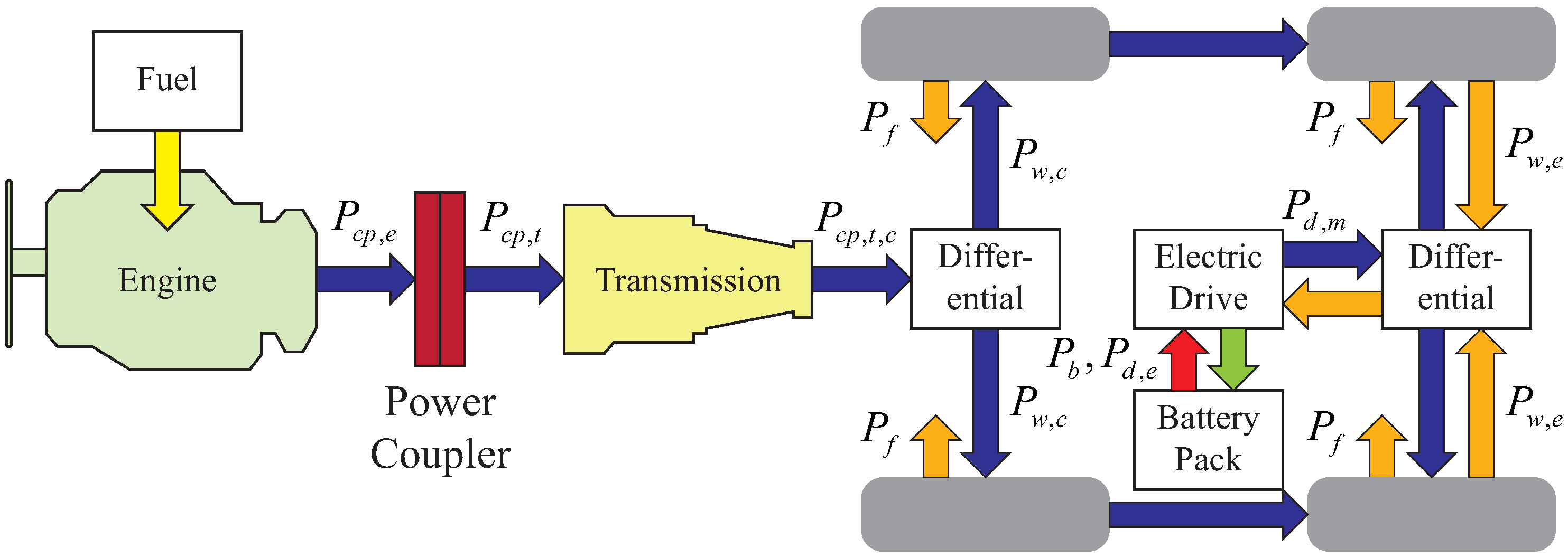
Figure 1 displays the potential power flows of the combined combustion-based and electrical-based propulsion systems. The vehicle is a through-the-road hybrid that can transfer mechanical power from the combustion engine to the battery through the road, as illustrated with the horizontal mechanical power (blue) lines from the left set of wheels (driven by the combustion engine) to the right set (connected to the electric powertrain); there is no driving-independent power transfer connection between the CP and EP. The electrical powertrain consists of a 225 kW induction motor, an AC-DC inverter electric drive system (EDS), and a 59.6 kWh lithium-Ion battery, common sizes already commercially available for light vehicles [
19]; the EP alone cannot provide for all driving duties. The hybrid truck tractor is modeled with the original 15 L engine as well as downsized diesel engines of 11 L (261 kW maximum power) and 7 L (149 kW maximum power).
The vehicle power management chooses the power flows of the CP and EP to both move the vehicle and consume kinetic energy to recharge the battery. The management control problem is a switched control problem since both the electric drive system and battery have unique dynamics based on the direction of the power flow. Switched control problems have been widely studied for a range of applications, cf. [
20,
21]. The EP has two modes of operation: EDS motoring/battery discharging and EDS generating/battery charging. The combined CP and EP power management is performed using a distributed switched system control introduced in [
19]. Accessory power loads are not considered, since they are often taken as constant values [
18], and our focus is on the dynamic power delivered to drive the vehicle. The component models and control cost functions are presented next. The different components are connected together using complicating variables, where the vector of complicating variables is
:
is the power at the CP transmission output,
is the CP transmission output angular velocity,
is the EP motor electrical power, and
is the EP motor angular velocity.
2.1. Combustion Engine Powertrain
The CP includes the diesel engine, transmission, and power coupler that joins them. The 15 L, 11 L, and 7 L diesel engine output power and fuel consumption models are derived from the data provided in GEM [
18]. The power and fuel consumption are algebraic models since the dynamics of the engine are much faster than that of vehicle motion:
where
is the maximum engine power regulated by
to obtain the output power
,
is the fuel mass flow rate,
is the engine angular velocity regulated by
,
and
are the lower and upper limits of
,
is the time constant of engine speed response, and
and
are fit coefficients. The forms of Equations (
1) and (
4) were determined empirically from the fitting of experimental engine data given in [
18]. Equation (
2) is a typical regularization to define control inputs over the unit interval to ease eventual numerical optimization. Equation (
3) prevents sudden changes in engine speed when it is decoupled from the transmission. The modeling parameters for Equations (
1)–(
4) for each engine are listed in
Table A1 and
Table A2 in
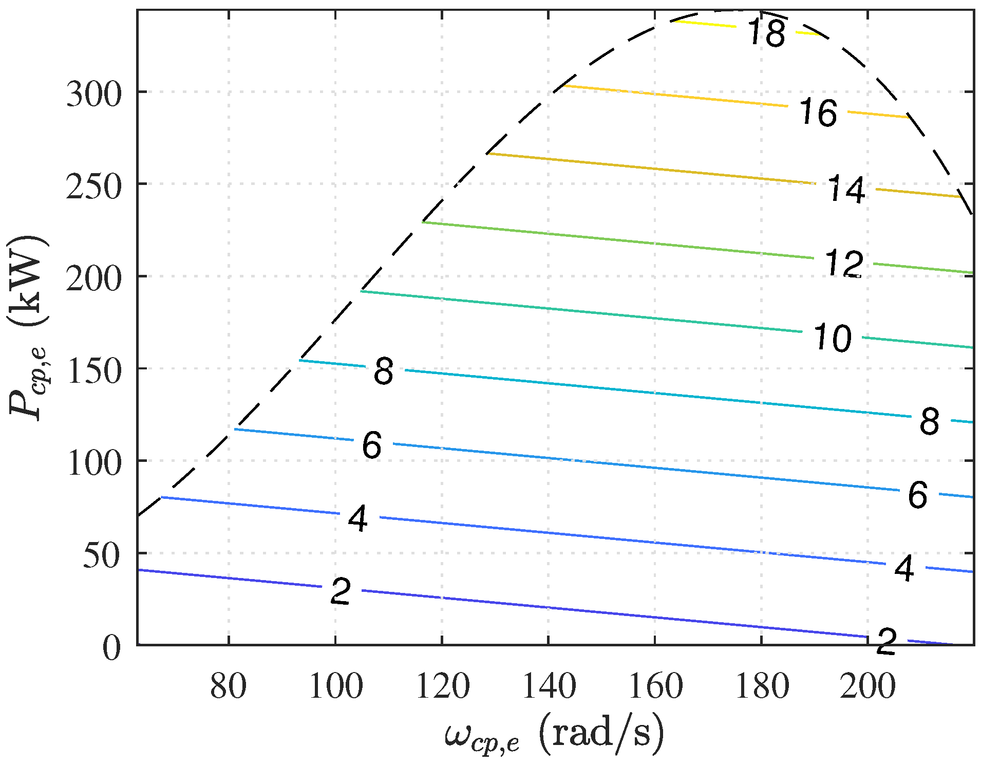
Appendix A;
Figure 2 shows the resulting maximum power curve and fuel flow contours for the 15 L engine.
The power coupler between the engine and transmission is an idealized device that transitions between the open and closed states in a nonzero finite time. In the open state,
is not transferred to the drive wheels, and the engine speed and transmission speed are independent. The open-to-closed transition is initiated when the time derivative of the vehicle longitudinal velocity reference (described in
Section 4) is increasing more than
m/s
over time, resulting in power transfer across the coupler:
where
is the power at the transmission input,
is the angular velocity at the transmission input, and
provides for starting the vehicle from zero velocity. The power coupler is considered closed when the transmission speed satisfies
. Upon closure,
and
(the latter constraint removes the choice of
). Conversely, the power coupler transitions from closed to open when the velocity reference is decreasing by at least
m/s
or more or the vehicle is stopped. The logic was sufficient to operate the original truck in simulation and is applied to the hybrid trucks as well. The forthcoming control regulates the engine power and speed such that
is sufficient to begin motion given rolling resistance, slopes, etc.
The transmission is a CVT with a gear ratio,
, the same span as the stepped transmission in [
18]. The output speed of the transmission is
, and the output power is idealized as
. The transmission is connected to the remainder of the vehicle with the complicating variables,
and
, which represent the power provided by the CP and the angular velocity at the transmission output, respectively:
where
,
is the vector of all complicating variables listed previously,
is the final drive gear efficiency between the transmission output and axle, and
and
are appropriate constant matrices needed for the control formulation in
Section 3.
The CP power management optimal control problem is
subject to Equations (
1)–(
6) and convex and compact variable bounds, where
is the power management prediction horizon,
is the current time, and
weighs the fuel use penalty. We note that penalizing fuel use is equivalent to penalizing CO
2 emissions as in [
18].
2.2. Electrical Powertrain
The electrical powertrain consists of the battery and EDS operating together. The EDS is a 225 kW maximum power induction motor coupled with a bidirectional AC-DC inverter. The EDS can either operate in motoring mode to propel the vehicle or battery regenerative mode to consume excess vehicle kinetic energy. The mode is controlled by a switched variable,
, that is 0 when motoring and 1 when generating. The EDS electrical dynamics are much faster than the vehicle motion dynamics and are modeled algebraically with motoring electrical power
:
Generating is modeled similarly with
:
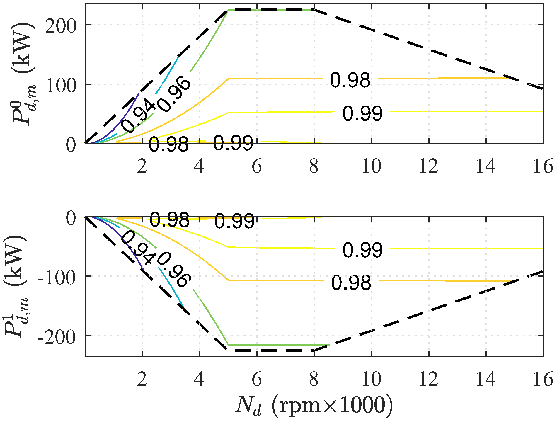
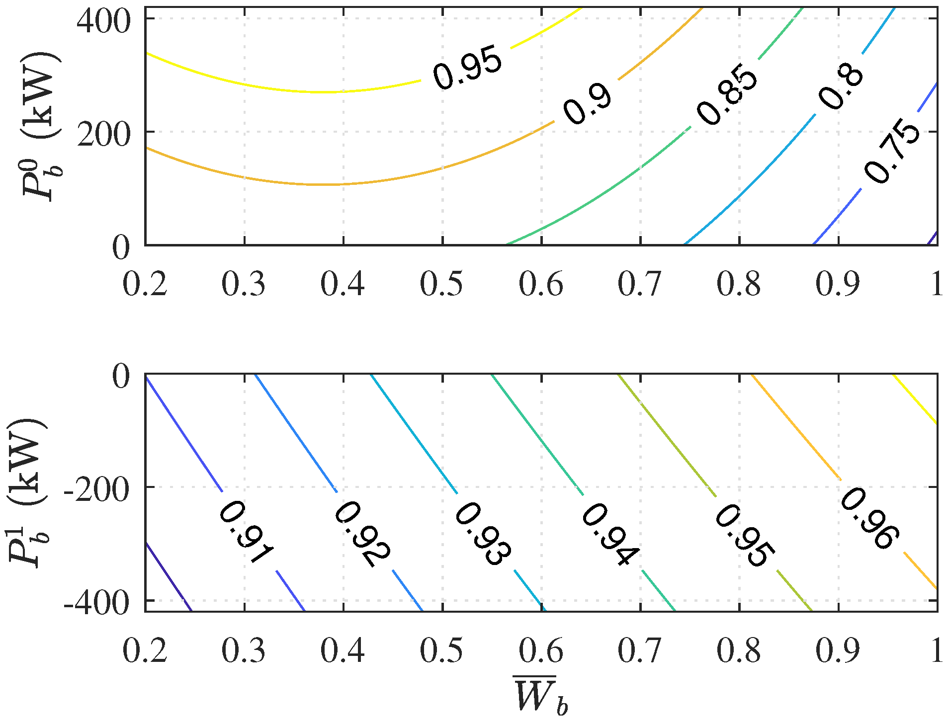
is the propelling/generating motor power transfer efficiency, shown in
Figure 3, developed from induction motor modeling, field-oriented control, and field-weakening control methods in [
22,
23] using data in [
24]:
where
is the motor shaft angular speed,
is the inverter efficiency,
captures the field weakening above the rated speed
rad/s,
and
are motor-parameter-derived constants,
is a regularization term to prevent division by zero at zero speed and/or zero mechanical power, and
regulates the maximum mechanical power, given in Equation (A1) in
Appendix A, in motoring and generating, respectively. The rated speed denotes the separation point in motor control: below the rated speed, the motor operates under field-oriented control with the maximum power set by the stator current limit and above the rated speed, the motor operates under field-weakening control where the maximum power begins to decrease linearly after
rad/s due to a maximum voltage limit.
Since there is not a single mechanical power value to use to connect with other components, a mode-weighted mechanical power value,
, is formed:
The lithium-ion battery that is connected to the EDS inverter to supply and absorb energy stores 59.6 kWh. The battery has two modes of operation, discharging and charging, which correspond to the EDS motoring and propelling modes. The mode switched dynamics are
where
is the state of charge (SOC),
is the battery’s maximum energy,
is the battery mode switch variable with
for discharge and
for charge,
is the mode-specific battery power with
kW for discharge and
kW for charge,
is the discharge/charge efficiency, and
/
and
/
,
, are discharge/charge fit coefficients.
Figure 4 displays the discharge/charge efficiencies from values in
Table A3 in
Appendix A, which was sourced from data in [
24].
The battery power is rate-limited to prevent battery damage from high frequency operation:
where
kW/s is the power rate limit magnitude determined from previous electric vehicle work [
24].
The battery and EDS are joined together by mode-specific connections
and the overall EP is connected to the complicating variables,
and
, with
where
and
and
are appropriate constant matrices needed for the control formulation in
Section 3.
The EP can operate in either motoring/discharging or generating/charging modes, which results in a switched optimal control problem:
subject to Equations (
8)–(
19) and convex and compact variable bounds where
is the penalty weight on the deviation of the SOC from the desired value.
2.3. Vehicle Operation Motion
The total vehicle includes the 6x4 truck tractor and trailer. The vehicle dynamics are modeled using energy conservation applied to point-mass, linear motion:
where
(
v is velocity),
is the drag force power,
is the rolling resistance,
is the power due to the body gravity force,
is the wheel power from the CP,
is the wheel power from the EP,
is the total frictional braking power,
is the vehicle mass including load,
is the product of the vehicle frontal area and drag coefficient,
is the tire rolling resistance,
is the ambient air density, and
is the road grade angle. The total truck tractor and trailer braking is proportional to the velocity:
where
is the maximum braking power,
is the maximum velocity, and
controls the applied braking power; note that a braking force is applicable at zero velocity.
The vehicle is joined to the CP and EP with complicating variables,
,
,
, and
:
where
is the angular velocity of the axle shafts,
is the wheel radius,
is the final drive ratio between the CP and axle,
is the final drive ratio between the EP and axle,
, and
and
are appropriate matrices needed for the control formulation in
Section 3. All vehicle parameters are listed in
Table A4 in
Appendix A.
The vehicle motion optimal control is to perform velocity reference tracking and frictional braking management. The control problem is
subject to Equations (21)–(
23) and convex and compact variable bounds where
weighs the deviation of the tracking from the reference
, and
weighs the use of friction braking to make regenerative braking preferred.
3. Distributed Control
The total vehicle power management must coordinate the combustion powertrain and electrical powertrain composed of the battery and EDS to meet the vehicle driving demands. The continuous-time component level control problems are approximated in discrete-time with a time step of
h using forward-Euler and trapezoidal numerical integration. The discrete-time control problems are solved in a receding horizon and distributed manner using the method presented in [
19] that is based on the popular alternating direction method of multipliers. To apply the method in [
19], the discrete-time component level cost functions are expanded to include the complicating variable connection constraints and a penalty on the connection constraint violation, resulting in the optimal control problem:
subject to
where
k is the time index;
N is the prediction horizon;
i indicates the component;
is the trapezoidal numerical integration representation of the cost function;
with
, where
is the state vector,
is the algebraic variables vector,
is the continuous control inputs vector, and
are the mode switches;
, with
denoting the complicating variables at
;
is the feasible region that is dependent on
, the initial state, and includes the dynamic and algebraic constraints and convex and compact variable bounds. With respect to the distributed control formulation,
is the dual variable, and
is a penalty parameter. The distributed solution method in [
19] iterates until the convergence conditions are met:
where
is the Kronecker product that results in an
matrix with a diagonal arrangement of
blocks repeated
N times,
is a similar Kronecker product to
,
l is a solution algorithm index,
is the number of connected components, and
and
are tolerances.
The EDS and battery are both switched components and have control problems that include discrete-valued mode switches. To avoid the computational complexity associated with discrete-valued mode switches [
20], the embedding method is applied, where
are relaxed to
, i.e., replaced with
. The resulting problems with all continuous-valued variables are embedded optimal control problems (EOCPs). If an EOCP solution results in any
, then the embedded solution must be projected back to
, and the projected optimal control problem (POCP) must be solved to obtain the control inputs to be applied. Here the projection utilizes the connection power values. For the EDS when
, if
, then the mode is propelling and generating otherwise. If projection is necessary, the distributed control is solved a second time with the projected mode values enforced. The optimal control problems formulated for the distributed solution meet the conditions for the existence of an EOCP solution and convergence of the distributed solution as outlined in [
19,
20].
4. Control Simulation
The Class 8 heavy-duty tractor truck with a trailer is simulated over three different driving cycles while transporting the maximum load of
kg: a trapezoidal driving cycle, the California Air Resources Board Highway’s Heavy-Duty Diesel Transient driving cycle with varying road angles, and the new European driving cycle. The latter two driving cycles are used to evaluate the hypothesis. The maximum load is chosen since it puts the most stress on the powertrain and control as well. The simulation time step is
s, and the prediction horizon is
. The distributed control is applied with
. We do not assume that the control has perfect knowledge of either the driving cycle velocity or road angle over the prediction horizon. The driving cycle velocity is linearly extrapolated from velocity at the current time and the requested velocity. These velocities are squared to create the reference kinetic energy:
where
is the current velocity at
, and
is the desired velocity that is delayed to one step ahead (the velocity is delayed since the velocity cannot instantly change). The road angle is not linearly extrapolated over the prediction horizon like the velocity; rather, the angle value at
, the driving cycle time associated with the start time of the current control calculation, is held constant over the prediction horizon.
The control of the different truck tractor powertrains utilizes the same component cost function penalty weights that were chosen after experimentation:
,
,
, and
where
is the minimum SOC, and
;
penalizes the decrease of the SOC more as it falls further below the reference value but does not penalize lowering the SOC, i.e., the use of the battery, when the SOC is above the reference. The starting SOC in all simulations is 0.8. Further, the simulations are performed in units of m, kg, W, radians, and seconds. The 15 L original ICE powertrain is referred to as 15L-ICE, and the hybrid vehicles are referred to by engine displacement as 15L-H, 11L-H, and 7L-H.
4.1. Trapezoidal Drive Cycle
The trapezoidal driving cycle consists of a 35 s constant acceleration to
m/s (25 mph), a 5 s constant velocity portion, and then a constant deceleration to zero over the final 35 s. The short time profile is meant to demonstrate the operating behavior of the powertrain compared to much longer regulatory profiles with many acceleration/deceleration events.
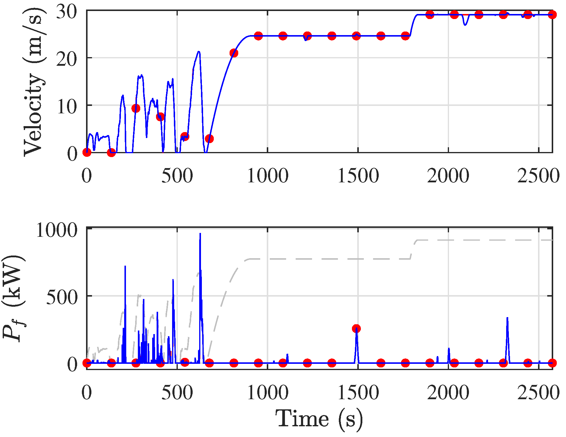
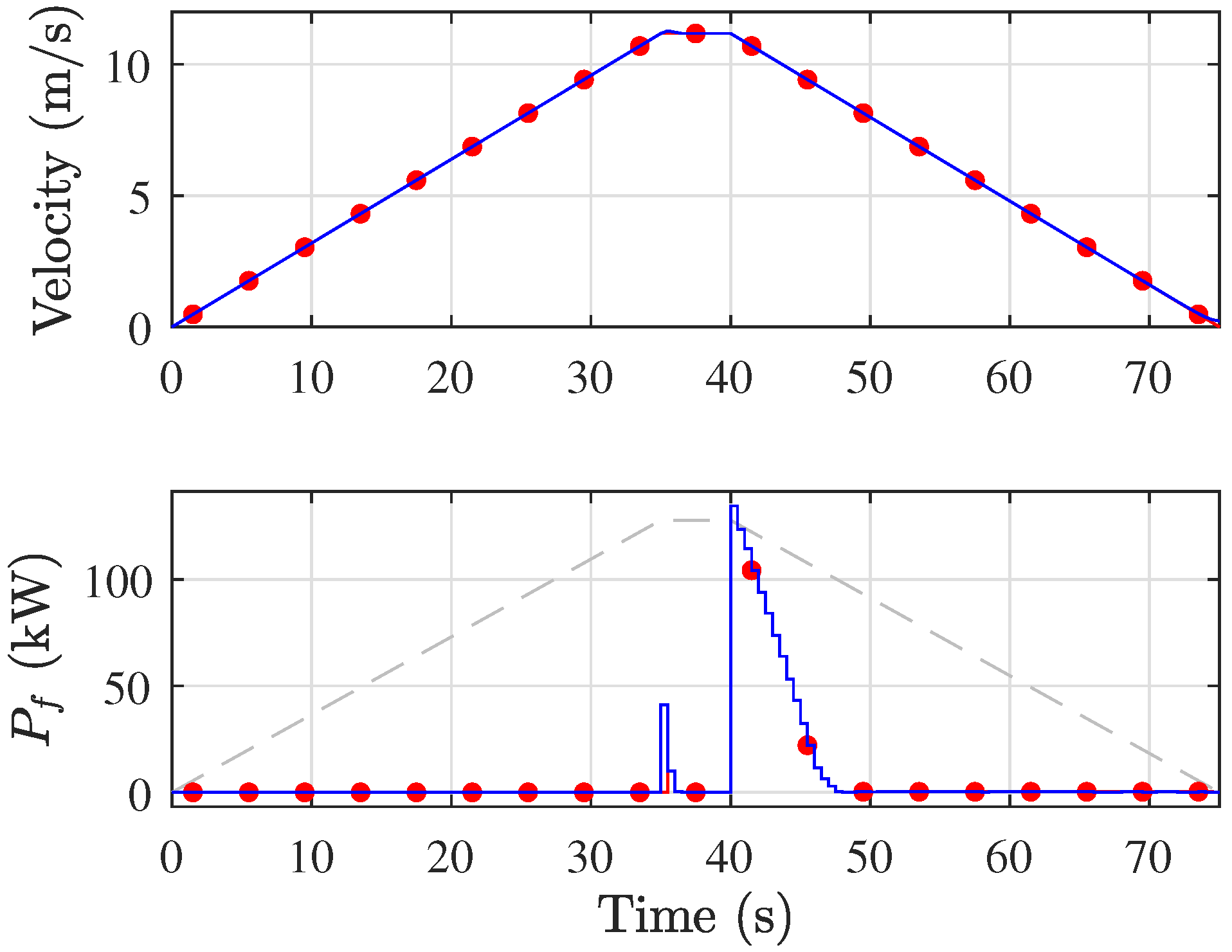
Figure 5 shows the performance of the 15L-H over the velocity profile, and
Table 1 shows the mean absolute percentage error (MAPE), the 2-norm normalized error N2NE (the 2-norm normalized error is equal to
), the final battery SOC, and the total fuel use. All of the powertrains result in acceptable velocity tracking with the greatest MAPE of 0.78% and an N2NE of 0.34%. The hybrids have effectively the same SOC at the end of the profile and a lower fuel use than the 15L-ICE, with 15L-H 87.3% less, 11L-H 87.7% less, and 7L-H 83.1% less. Even over the short trapezoidal profile, the ability to use the battery and regeneratively brake provides a benefit compared to the 15L-ICE.
To better understand the hybrid operation, the 15L-H CP and EP performance is examined.
Figure 6 shows the engine power, cumulative fuel use, and engine speed of the 15L-H. The power rises with velocity, stays relatively unchanged over the constant velocity portion while providing motoring power, and then the engine is idle during deceleration. The 15L-ICE shows a much larger, nearly linearly increase in power with velocity during the acceleration portion since there is no EP to provide support. The maximum 15L-H engine power is
kW, while the 15L-ICE is
kW, an increase of
. Further, the maximum 11L-H ICE power is similar to the 15L-H value, but the 7L-H value is lower at
kW.
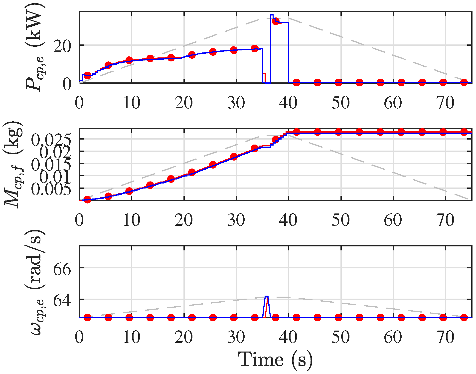
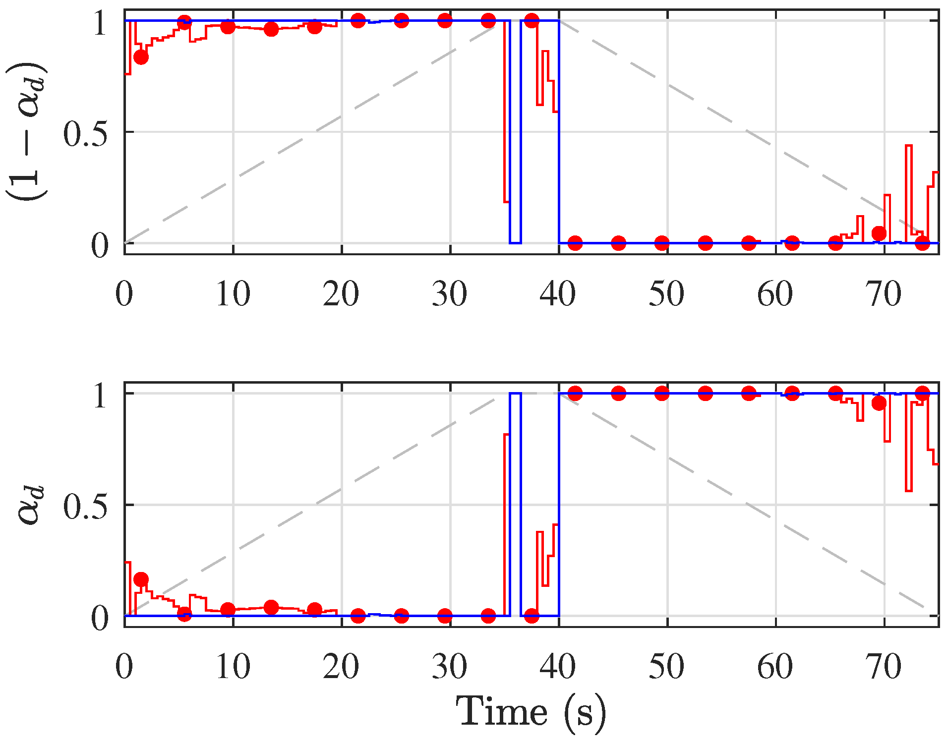
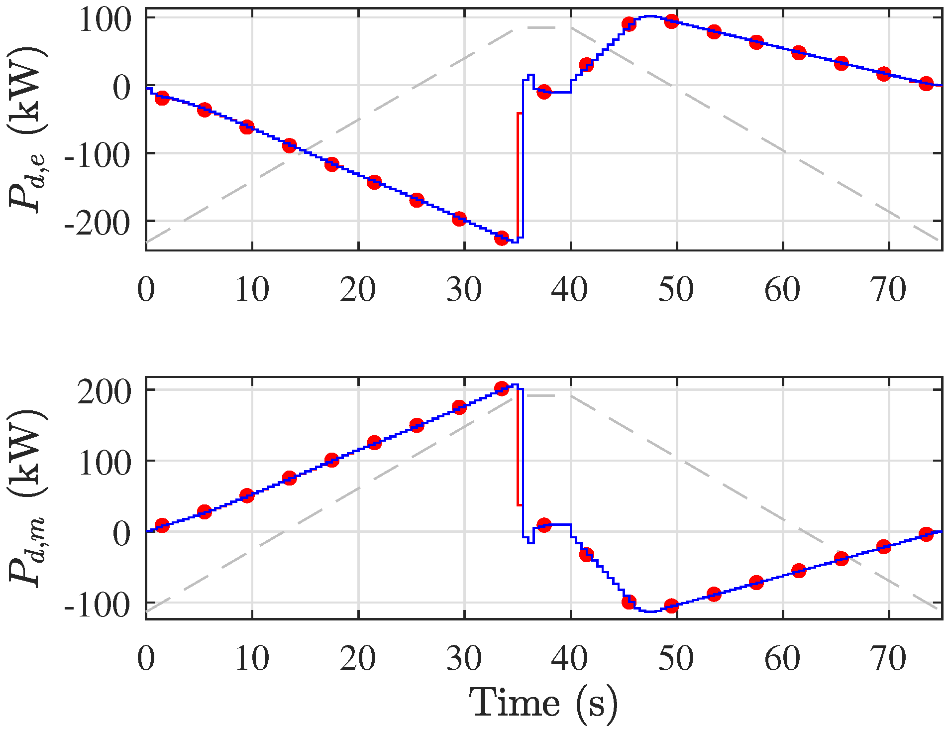
Figure 7 and
Figure 8 show the EP mode selection and EDS electrical power and mechanical power over time. In the mode over the acceleration, the first 35 s is motoring/discharging, meaning the CP and EP are working together to propel the truck. At 35 s, the embedded mode value is closer to generating/charging, but the projected value is motor/disgcharging, since the EP power connected to the vehicle is positive, indicating propulsive force. Over 35.5 to 36.5 s, the generating/charging mode is active in capturing vehicle kinetic energy; similarly, the mode is active during the entire deceleration portion, corresponding with the preference for regenerative braking and charging the battery. An additional numerical experiment with an enforcement of generating/recharging over
s showed that the initial transition from acceleration to constant velocity at 35 s is kept at motoring/discharging by the controller to save fuel, with a reduction of engine use; the use of the electric motor is constrained by the battery power rate limitation, resulting in the small use of frictional braking. EP mode projection was required 36% of the time (38.7% for 11L-H and 30.0% for 7L-H), thus bang-bang or switched solutions were obtained from the EOCP the majority of the time. The mechanical power in
Figure 8 rises with the overall powertrain demand over the constant acceleration portion of the cycle and turns negative during the regenerative braking over 35.5 to 36.5 s and 40 s onward. Frictional braking, shown in
Figure 5, is used at 35 s and during the first 7.5 s of the deceleration. Frictional braking is applied at 35–36 s to maintain the velocity tracking, given that the braking power rate limit and mode selection does not allow for sufficient regenerative braking otherwise. During the first 7.5 s of the deceleration, the frictional braking is active again because of the battery power rate limit. After 47.5 s, the battery charging power has reached a high enough value that the braking can be entirely regenerative. Similar EP trends are observed in the 11L-H and 7L-H results.
4.2. Regulatory Drive Cycles
Table 2 summarizes the results of the performance over the California Air Resources Board’s Highway Heavy-Duty Diesel Transient driving cycle (HHDDT) and the new European driving cycle (NEDC). The driving cycles are reported without and with a charge sustaining (CS) operation. A charge sustaining operation is achieved by enforcing a lower bound
that is dependent upon the remaining drive time and current SOC:
where
is the duration of the driving cycle, and the value 2 was tuned to give a suitable final charge. The charge sustaining inequality is only applied when
, the power coupler is closed, the change in reference velocity is less than
m/s between points over the prediction horizon, and the vehicle velocity is not more than
m/s less than the reference velocity at
.
Figure 9 shows the 15L-H performance on the HHDDT (the NEDC profile is more well known than HHDDT and is not shown due to space considerations). Very good tracking is demonstrated by the 15L-H, and frictional braking is only used briefly on the commanded deceleration segments when regenerative braking saturates.
Table 2 shows the hybridization results: significantly reduced fuel and a lower total energy use, where total energy includes the fuel energy plus additional energy from a 1 MW fast charger to charge the battery pack back to the original 0.8 SOC. The hybrid fuel savings are greater when CS is off, which is expected since the final SOC can be less than it is with CS. Without CS, the minimum fuel savings compared to the 15L-ICE is the 15L-H over the HHDDT at
%, and the maximum is the 7L-H at
% over the NEDC. With CS, the minimum fuel savings are
% over the HHDDT, and the maximum is
% over the NEDC. However, total energy savings without CS are less compared to using CS, indicating differences between the two approaches in how the battery is used and fast charger inefficiencies. Considering the velocity tracking, the 15L-H and 11L-H demonstrate that the MAPE and N2NE are similar to 15L-ICE. If the 7L-H powertrain is removed from consideration because of large MAPE and N2NE errors, then the maximum fuel savings are
% for the NEDC CS and
% for the NEDC without CS. In line with the CO
2 modeling approach adopted by the United States Environmental Protection Agency’s Greenhouse Gas Emissions Model [
18], tractor CO
2 emissions are taken to be directly proportional to fuel use, so the changes in CO
2 are the same as the fuel changes. The simulation data presented can inform and guide the commercial adoption of hybrid truck tractors as either retrofit or new products. The greater the energy savings, the faster the recovery of additional costs incurred through hybridization.
The regulatory driving cycle results, with respect to the tested profiles, support the hypothesis that a through-the-road hybrid with a reduced engine displacement will result in reduced fuel use, total energy, and CO2 emissions compared to the original vehicle. The results indicate that the combination of reduced engine displacement from 15 L to 11 L, hybridization, and CS operation results in nearly as good or better velocity reference tracking while achieving lower total energy, fuel use, and emissions compared to the 15L-ICE and 15L-H. We caution that additional evaluations of different driving cycles are needed to understand the wider applicability of this conclusion.
4.3. Penalty Weight Study
Table 3 shows the results of changing the velocity reference tracking and fuel use penalty weights without CS,
and
, respectively. We observe that increasing/decreasing
alone results in better/worse reference velocity tracking. Similarly, increasing/decreasing
alone results in better/worse fuel economy and worse/better SOC. Combinations of changing
and
follow similar trends. These results demonstrate that there are many reasonable options for control tuning, and the values chosen for the previously presented results are not the only ones that may produce acceptable results.
5. Conclusions
The application of hybrid power to a Class 8 6x4 truck tractor with a high roof sleeper cab and a long dry van trailer was investigated under distributed switched optimal control and different engine sizings. The heavy-duty hybrid truck is a through-the-road hybrid with one axle driven by a combustion powertrain and the other axle driven by an electrical powertrain composed of an electric drive system and a battery with two modes of operation: motoring/battery discharging and generating/battery charging. Control-oriented power flow models were created for the combustion powertrain and given for the electrical powertrain. A recently developed distributed switched system control algorithm was used to manage the interactions between the combustion powertrain, the electric powertrain, and the vehicle operation. The algorithm is based upon the embedding method for solving switched optimal control problems with discrete-valued mode switches, such as the power flow direction of the electrical powertrain. A conventional 15 L displacement ICE-only truck and hybrid trucks with 15 L, 11 L, and 7 L engine displacements were simulated over test and regulatory driving cycles. The control tuning was kept consistent between all powertrains and tests to form a consistent basis of comparison. Hybridization results showed less fuel consumption, fewer CO2 emissions, and less total energy use, even accounting for the charge sustaining operation and energy needed to return the battery’s state-of-charge to the initial value, and the savings increase as the engine displacement is reduced. The drawback to the engine downsizing is that velocity reference tracking suffers over the regulatory cycles. The reasons are that the peak powers of the combustion and electrical powertrains do not align, resulting in less total deliverable power at certain engine speeds than is possible from the original 15 L ICE alone. However, the results indicate that the combination of a reduced engine displacement from 15 L to 11 L, hybridization, and CS operation results in nearly as good or better velocity reference tracking while achieving lower total energy, fuel use, and CO2 emissions compared to the 15L-ICE and 15L-H, supporting the hypothesis that improvements with hybridization and engine downsizing are achievable. We caution that additional different driving cycle evaluations are needed to understand the wider applicability of this conclusion.
Future work will include the incorporation of different electrical powertrains with peak power near that of the tested ICEs to produce a power curve similar to that of the 15 L ICE in an effort to reduce velocity reference tracking error while keeping significant energy savings; this will include the addition of a transmission between the axle and the current electrical powertrain. Different driving cycles will be evaluated as well to understand the broader applicability of the approach and potential benefits. Moreover, additional vehicle classes will be considered for hybridization to better understand the specific needs of commercial vehicle hybridization and how to best lower total operating costs. Further, additional optimization algorithm tunings are of interest to better understand the penalty weight effects on performance given that the control problem is nonlinear.


