Effective Permutation Encoding for Evolutionary Optimization of the Electric Vehicle Routing Problem

Abstract

This paper addresses the problem of route planning for a fleet of electric vehicles departing from a depot and supplying customers with certain goods. This paper aims to present a permutation-based method of vehicle route coding adapted to the specificity of electric drive. The developed method integrated with an evolutionary algorithm allows for rapid generation of routes for multiple vehicles taking into account the necessity of supplying energy in available charging stations. The minimization of the route distance travelled by all vehicles was taken as a criterion. The performed testing indicated satisfactory computation speed. A real region with four charging stations and 33 customers was analysed. Different scenarios of demand were analysed, and factors affecting the results of the proposed calculation method were indicated. The limitations of the method were pointed out, mainly caused by assumptions that simplify the problem. In the future, it is planned for research and method development to include the lapse of time and for the set of factors influencing energy consumption by a moving vehicle to be extended.

1. Introduction

1.1. Background

In order to meet social, economic and environmental challenges and adjust to global trends, it is necessary to implement a coherent and sustainable program for the development of transport systems, including: increasing competitiveness through integrated logistical solutions covering various means of transport; application of technologies ensuring the reduction of fuel consumption and enabling the use of alternative energy sources; adjusting transport policy to energy policy, aimed at improving its efficiency and giving it a pro-environmental character; and reduction of greenhouse gases and noise.

Electrically-powered vehicles are being promoted as a key factor in building a sustainable mobility system and there are indications that they will break the long-term dependence of mankind on internal combustion engines and diesel fuel as a means of meeting its transportation needs. Increasing the use of electric vehicles, in particular when powered by renewable energy, can play an important role in reducing greenhouse gas emissions and in the transition to a low-carbon economy in the future.

The growing popularity of electric drives in passenger vehicles and delivery trucks has prompted researchers around the world to turn their attention to electric drive operation, and to search for ways of efficient use in transportation and methods of managing fleets of such vehicles. As a result, knowledge in the area of Vehicle Routing Problems (VRPs) that has been developed for decades has reached a new level that includes environmental aspects. This is part of a broader development trend, the so-called (in the literature) Green Vehicle Routing Problem (G-VRP) or Environmentally Friendly Vehicle Routing Problem (EF-VRP) [1].

1.2. Literature Review

Electric vehicles (EVs) have unique characteristics that limit the application of classic VRP methods. Electric Vehicle Routing Problems (E-VRPs) examined in the literature often take into account many additional aspects, including maximum vehicle battery capacity, maximum range per charge, charging time, and infrastructure parameters such as charging station availability [2]. An extensive review of the different variants of the E-VRP problem is found in [3].

Many researchers place electric vehicles in a broader group called Alternative Fuel Vehicles (AFV), which includes vehicles powered by biodiesel, ethanol, hydrogen, methanol, and natural gas. These fuels strongly limit the vehicle range given the current state of technology. The concept of the Alternative Fuel Vehicle Routing Problem (AF-VRP) was introduced in the publication [4], whose authors deal with biodiesel-powered vehicles.

A characteristic distinguishing electricity from other alternative fuels is the nonlinear battery charging time. This phenomenon is particularly noticeable when batteries are charged to above 80% of their capacity [5]. The charging time from 80 to 100% is so long that during a working day, it is more cost-effective to charge the batteries more frequently to the 80% level than to charge them less frequently to the 100% level. Models that take these aspects into account are called Electric Vehicle Routing Problems with Nonlinear (E-VRP-NL) Charging Functions. In [6], three variants of the charging station were adopted: fast, moderate, and slow. The uncertainty and risk of queues at the stations have been included as a new occurrence, leading to a dynamic routing problem. Many authors address the E-VRP-NL problem simultaneously with the analysis of battery charging strategy and the development of the charging station network [7,8,9]. The consideration of the effect of a vehicle load level on its range is also an interesting expansion of the model [10].

As further restrictions and criteria are introduced, theoretical models proposed by authors are becoming more complex. The high complexity of theoretical models makes the methods for finding optimal solutions require using heuristics and limits their practical applicability.

Mixed integer linear programming (MILP) introduced by Gheysens [11] is a well-established (in literature) method of encoding VRP solutions. In this approach, the solution to the problem is encoded in a binary matrix, which assumes a gigantic size for non-trivial problems. Therefore, matrix-based encoding of VRP problems does not support the presentation and interpretation of results by the user. For the MILP method, a solution is usually a sparse matrix, which leads to the need to assume many constraints and excessive computation time for relatively simple problems. As a result, an optimization algorithm must check each solution against the requirements:

• Each customer is visited exactly once (2n repetitions of the constrain test, where n is the number of customers visited);
• All customer demands are satisfied (n repetitions of the constrain test);
• The load and capacity of vehicles are consistent;
• Goods travel routes are synchronized with vehicles’ routes (n²—n repetitions of constrain test);
• Number of vehicles dispatched and provided in the depot are consistent;
• The route is not disconnected.

The MILP method is widespread in many varieties of VRP problems, and each additional complexity of the model imposes further constraints. When considering multiple types of vehicles [11], multiple types of goods [12], time windows [13], or dynamically changing demand [14], the number of checked conditions multiplies.

The MILP method dedicated to vehicles with alternative energy sources was proposed in [4]. The authors extended the set of assumptions by adding conditions:

• Non-negative level of fuel in vehicles;
• Sufficient fuel to continue the journey at each point of the route; and
• The amount of replenishment at stations.

Matrix coding is also commonly used in E-VRP problems. The study conducted by [3] indicates the very high popularity of the MILP method based on the analysis of 175 literature items. The method is readily adapted by the authors of the publications to various types of problems, e.g., charging time and variable travel time [15], time windows and path flexibility [16], and nonlinear charging time [5,6,17].

An alternative to matrix modeling of the vehicle route is the permutation notation. It is important to distinguish between the use of permutations to represent the solution obtained with the MILP method and the direct execution of calculations on permutation codes. The first of these two approaches appears in many of the publications mentioned above. The second proposal was applied first to the relatively simple Traveling Salesman Problems (TSP) [18], then to the increasingly complex VRP. The linear programming approach was judged to be too slow when solving TSP [19]. The authors pay attention to long computation times and the need for a lot of memory space. In the work [20], a method of permutation coding of the route of many vehicles was proposed. It was noted that such coding allows for simultaneous modeling of the divisions of visited points between vehicles. This method is applicable to VRP, but has not yet been adapted to electric vehicle route planning. In the methods review [3] the permutation coding is omitted.

The article [21] reviews the coding methods in terms of the possibility of using evolutionary algorithms for optimization. The effectiveness of combining permutation coding with the evolution optimization of the TSP was noted. In the work [22], the mutation operators acting on permutations were compared. The conclusions point to the inversion, displacement, and pairwise swap methods as computationally fast solutions.

1.3. Contribution of this Paper

The article presents a mathematical model for the E-VRP problem with a simplified consideration of the nonlinear charging time problem. The simplification results from the omission of the problem of time in the model. Based on the literature review, it was assumed that a rational level of charge obtained in the station is 80% of the maximum capacity of the battery.

A novelty in the developed model is the use of two levels of coding solutions. At the basic level, the solution is represented by a numerical sequence that directly defines the order of the visited points along the route, including the CS and the depot point. As the model is designed with the aim of conducting optimization calculations as fast as possible, a higher level of coding has been introduced, where only the order of visited customers is taken into account. The main advantages of this approach are that in every possible solution:

• Every customer will be visited;
• There are no returns to a previously visited customer;
• The route is continuous.

The above features are not obvious for other encoding methods (MILP for example) and often require many additional constraints, the fulfilment of which must be verified. The comparative tests described in Section 4 show that permutation encoding is generally more efficient than the matrix-based approach, both in terms of the speed and quality of the results obtained.

An important element of the developed model is the encoding algorithm which, on the basis of permutation coding, enables determining when the vehicle must replenish energy and at which station and when it must return to the depot in order to load the goods.

The proposed approach to the E-VRP makes it combinatorial. Therefore, it is advisable to use an evolutionary algorithm as a method to find the optimal solution. For this purpose, appropriate genetic operators have been designed. When planning the optimization calculations, you can appreciate the advantages of the proposed permutation coding. Generating a random first population is a simple combinatorial problem and all obtained solutions are feasible. There is no need to use various penalty functions that help maintain evolution in the area of feasible solutions. In the test, calculations roulette selection and the order crossover method were used. The crossover of permutations generates solutions that are always feasible, which affects the running time of the algorithm. Mutation of permutations is also performed with a simple numerical operation.

The problem with permutation coding of VRP is that the points sequence has to be broken down into parts served by different vehicles. In the case of problems focused on the control of vehicle loading, this division results from the amount of goods needed by consecutively visited customers. The point (customer) where the load capacity of one vehicle is exceeded must be served by the next vehicle. However, the application of permutation encoding to the E-VRP requires developing a method that considers additional matters:

• The need to recharge the battery while travelling a route;
• Supervision of the range of a vehicle—preventing it from “getting stuck” on the route;
• Selecting a charging station and taking into account the additional distance that the vehicle has to travel.

This paper has the objectives to implement the above functions by permutation encoding and to investigate the performance of the solution in real-life conditions.

Vehicle parameters, such as range, carrying capacity (payload), and battery charging time are variables in the theoretical model, but in the test calculations, they are chosen in a way that corresponds with the current state of the art. The goal is to verify not only the validity of the theoretical model, but also its effectiveness in the computational solving of real problems in a reasonable time.

2. Problem Formulation

2.1. Assumptions

The problem addresses routing for multiple electric vehicles. All vehicles share a common task and are managed by a single forwarder. The theoretical model has been developed, starting with the following assumptions:

• A fleet of identical EV is waiting in the depot to set off to customers and deliver to each of them a certain quantity of goods that they ordered;
• All EVs set off from the depot with 100%-charged batteries, which allows covering the established distance;
• The carrying capacity of a single EV is limited by a fixed value which may not be exceeded;
• No customer requests more than the maximum capacity of one vehicle;
• In the area handled by the vehicle fleet there are charging stations allowing the batteries to be recharged in an acceptable time to level 80%;
• Each charging station can handle multiple vehicles at the same time;
• The route plan for each vehicle must include any need to replenish energy and return to the depot after the goods have been delivered;
• Between points on the map (depot, charging stations, and customers), the route distances that the vehicle must cover are given;
• The distance of a route between any two points is affected by the existing road infrastructure and is determined from empirical data or navigation. The route distances can be expressed in km, or in time units, which will allow the inclusion of additional aspects related to speed limitations on certain roads and delays due to traffic lights and periodic traffic congestion. Obviously, time data is more susceptible to variability than distance expressed in units of length.

The model does not take into account the wear of batteries and the associated reduction in capacity.

Another simplifying assumption is the linear decrease in the vehicle range as the distance is travelled. The effects of speed and vehicle loading are not considered. The model also does not consider the quality of the road surface, the slope of the route, the traffic volume, or the weather.

2.2. Mathematical Model

The following notations are used in the proposed mathematical model:

s = 1, 2, …, S	numbering of charging stations,
c = 1, 2, …, C	numbering of customers,
P	the total number of nodes considered in the planning (the depot, CSs and customers),
b, b1, b2 = 1, 2, …, B	numbering of elements in the solution vector y,
z = (z1, z2, …, zC)	vector of orders,
Lmax	carrying capacity of a single EV,
Rmax	range of EV with fully-charged batteries,
R80	range of EV with 80%-charged batteries—after visiting CS,
D = (di,j)P × P	the distance matrix, with rows and columns correspond to nodes, as shown in the Figure 1.

The task is to find a travelling route y to deliver ordered good to all the customers at the minimum distance:

$$\min D\left(y\right)={\displaystyle \sum _{b=1}^{B-1}{d}_{y_b,y_{b+1}}}$$

(1)

where y = (y₁, y₂, …, y_B) is a vector of decision variables, whose components represent the numbers of nodes successively visited by one or more vehicles, B is the number of visited nodes depending on the number of returns to the depot and the number of visits to the charging stations. The customer numbers are separated with CS numbers and depot station (number 1) in selected positions.

It should be noted that we define the range of variable values as a closed interval: [], which is understood as a certain subset of natural numbers. Therefore, we interpret the values in the vector y as EV is visiting in the step b:

y_b ∈ [1, P]—one of all considered nodes,

y_b ∈ [S+2, P]—one of the customers,

y_b ∈ [1, S+1]—the depot or one of the CSs,

y_b ∈ [2, S+1]—one of the CSs.

The solution y should satisfy the following constraints:

$$B\ge C+2$$

(2)

$$\forall b_1,b_2\in \left[1,B\right]:y_b\in \left[1,P\right]$$

(3)

y₁ = y_B = 1

(4)

$$1<b_1\ne b_2<B:y_{b_1},y_{b_2}\in \left[S+2,P\right]\Rightarrow y_{b_1}\ne y_{b_2}$$

(5)

$$\forall b_1,b_2\in \left[1,B\right]:y_{b_1}\in \left[1,S+1\right]\Rightarrow {\displaystyle \sum _{b=b_1}^{b_2-1}{d}_{y_b,y_{b+1}}}\le \delta \cdot R_{max}+\gamma \cdot R_{80}$$

(6)

where δ is the quantity of values 1 and γ is the quantity of values from the set {S+2, 3, …, S+C+1} in the segment of the vector y: $\left(y_{b_1},\dots ,y_{b_2}-1\right)$.

$$\forall b_1,b_2\in \left[1,B\right]:y_{b_1}=1\Rightarrow {\displaystyle \sum _{\underset{y_b>S+1}{b=b_1+1}}^{b_2}{z}_{y_b-S-1}}\le \delta \cdot L_{max}$$

(7)

Constraint (2) means that the vector y must contain at least enough elements to leave the depot, visit all clients and return to the depot; (3) defines the set of elements of the vector y; (4) means starting and ending the route at the depot. There may be additional values of 1 in the vector y, which means that the route consists of several loops; (5) ensures that each customer is visited only once; (6) checks if any part of the route after charging at the depot or CS is not greater than the range obtained from charging; (7) controls the vehicle loading level in relation to customer demand.

Additional assumptions relate to the definition of the problem:

$$\forall c\in \left[1,C\right]:z_c\le L_{max}$$

(8)

$$\forall j\in \left[S+2,P\right]:d_{1,j}\le R_{max}\vee \exists i\in \left[2,S+1\right]:d_{i,j}\le R_{80}$$

(9)

Constraint (8) ensures that no request exceeds the maximum capacity of a vehicle; (9) checks that no customer is too far from the depot or one of the charging stations.

The problem described by the model can be solved directly by evolutionary methods. However, the search for a vector y that satisfies all the constraints and minimizes the function (1) may be long term and give results far from the global optimum. Coding a solution in the form of a vector y is not computationally efficient; therefore, the aim of the presented research is to find a coding method that would narrow the search space to a set of acceptable solutions and thus speed up the calculations.

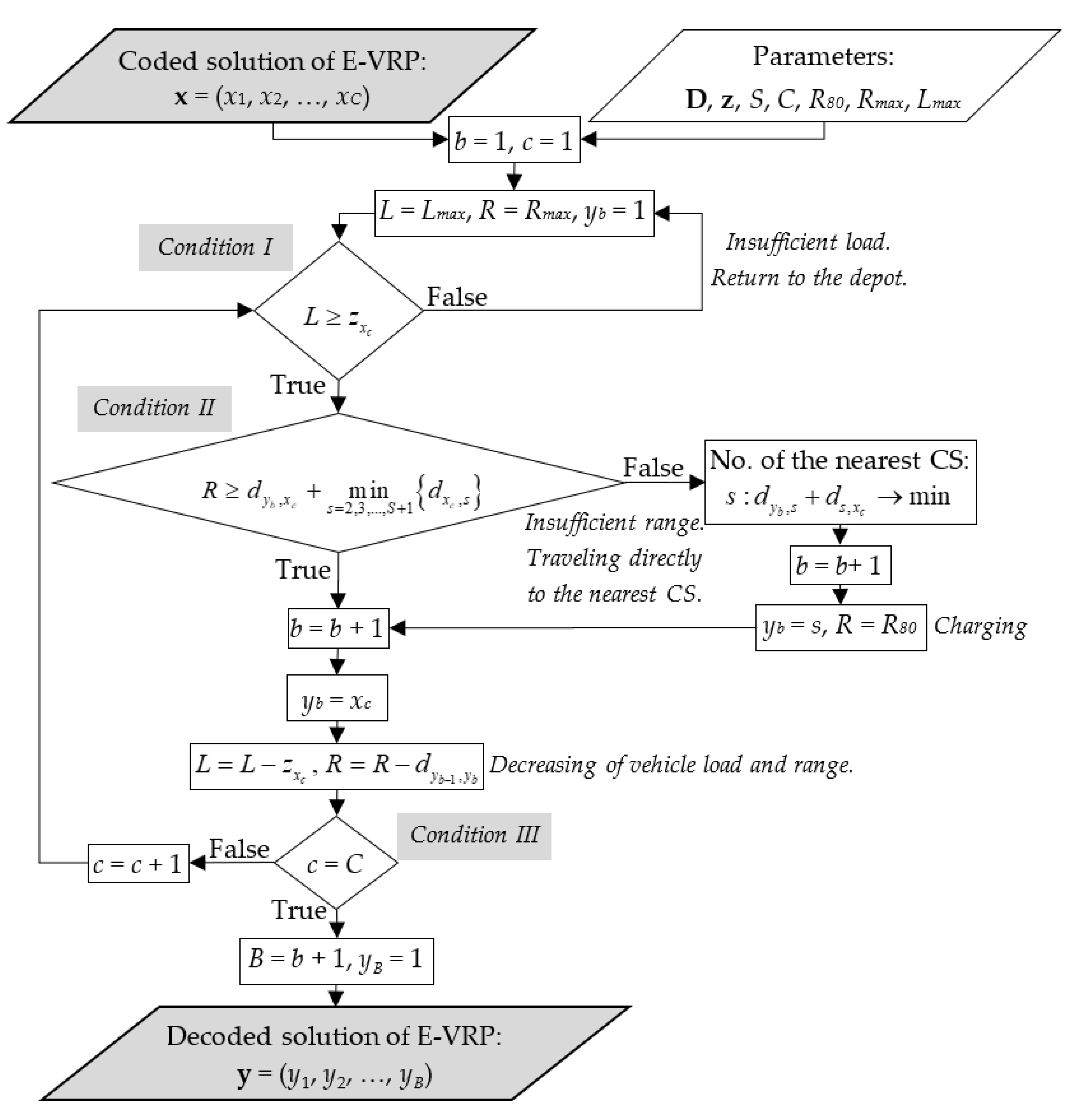
2.3. Permutation Encoding of Solution

The proposed solution is based on the conclusion that if we want to serve customers by covering the shortest possible route, we have to charge the battery and load goods as rarely as possible. In this case, for any given order of visiting customers, we can clearly determine when to replenish the load (i.e., visit the depot) and charge the battery (i.e., visit one of the CSs). In the proposed method, any solution to the E-VRP may be represented as a permutation of customer numbers:

x = (x₁, x₂, …, x_C),
∀c, c₁, c₂ = 1, 2, …, C: x_c∈[S+2, P], x_c1 ≠ x_c2

(10)

To find out when the vehicles visit the depot and CS’s, we need to decode solution x taking into account additional information such as the distance matrix D and the vector of orders z = (z₁, z₂, …, z_C).

The proposed function that decodes solution x is the computational algorithm presented in the Figure 2. Two indexes are used in the calculations. The index b numbers the elements of the result vector y. Index c numbers the elements of the input vector x. The algorithm includes three logical conditions that check: the quantity of goods (condition I), the vehicle range (condition II), and the end of the operation (condition III). As a result, calculations take fractions of a second even for large sets of customers. The tests performed in the Matlab environment allowed the conclusion that the performance enables using the algorithm in evolutionary calculations.

For example, we take the depot number 1, two charging stations numbers 2 and 3, and five customers with numbers 4, 5, …, 8. Let’s assume that:

• The maximum reach of the vehicle is 10;
• The maximum payload of the vehicle is 1;
• The charging station replenishes energy up to level 0.8;
• The encoded solution of the problem is a vector x = (7, 5, 4, 6, 8).

Assumed significant distances between points and the quantity of ordered goods are shown in Figure 3. The graph on the left shows the theoretical route that the vehicle would have to travel if the decoding function was not used. It can be seen that the total distance to be travelled according to solution x is 14, while the total requirement is 1.6. Therefore, a vehicle cannot cover this distance, and it cannot deliver goods to all customers in one loop without replenishing energy and cargo.

We can follow the operation of the decoding function.

Table 1. Calculation steps of the decoding function.

b	Vehicle Location yi	Vehicle Reach R	Vehicle Load L	c	Next Customer xc	Step Results
1	1	10	1	1	7	Conditions I and II—met. Travelling from 1 (the depot) to 7.
2	7	9	0.7	2	5	Conditions I and II—met. Travelling from 7 to 5.
3	5	6	0.5	3	4	Condition II—not met. Travelling to 3 (the nearest CS).
4	3	8	0.5	3	4	Conditions I and II—met. Travelling to 4.
5	4	5	0.1	4	6	Condition I—not met. Travelling to 1 (the depot).
6	1	10	1	4	6	Conditions I and II—met. Travelling from 1 (the depot) to 6.
7	6	6	0.8	5	8	Conditions I and II—met. Travelling from 6 to 8.
8	8	4	0.3	-	-	Condition III—met. End of route, return to 1.
9	1	-	-	-	-

shows the vehicle’s reach and load changes during the trip. The influence of testing conditions on the decisions about visiting the CS or returning to the base is visible. The vehicle sets off from the depot to customer 7, then travels to customer 5, then replenishes energy at charging station 3. After replenishing energy, it delivers the goods to customer 4 and returns to the depot because it has disposed of all the goods. The second vehicle sets off from the depot to customer 6, then drives to customer 8, and then returns to the depot. After decoding, we obtain vector y = (1, 7, 5, 3, 4, 1, 6, 8, 1). Charging station 2 is not used in this plan. Both vehicles can leave the depot at the same time. It is also possible that one vehicle returns to the depot, is loaded again, and begins another run. The allocation of tasks among vehicles is a separate problem that is not addressed in this paper.

3. Example Study

With the formulated model, example optimisation calculations were performed for the following set of points (Figure 4):

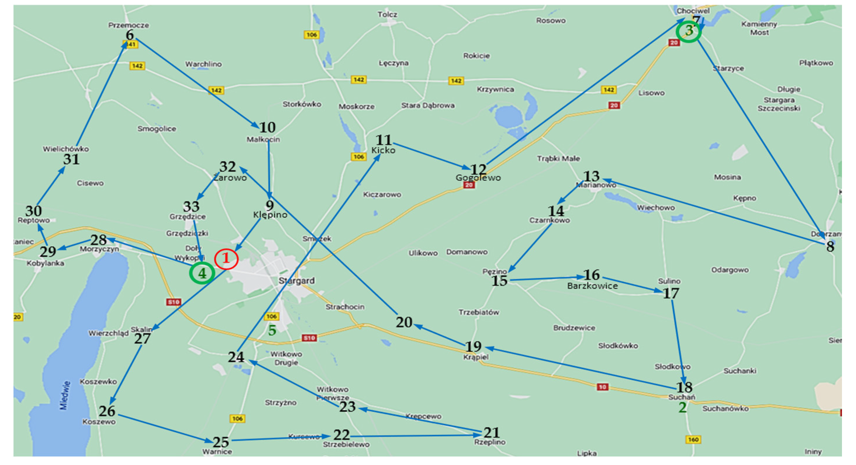
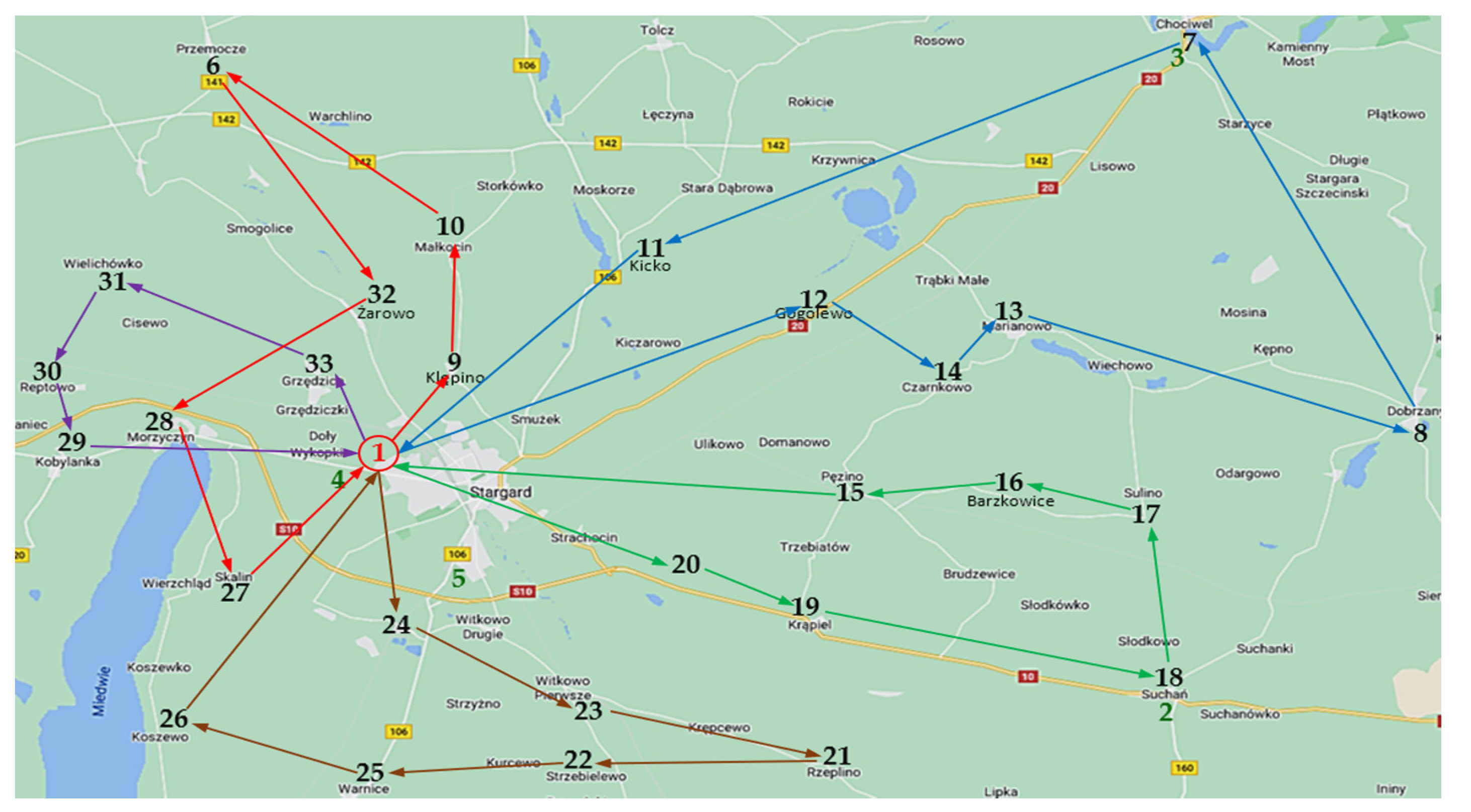
• Point 1—the depot—Stargard City located in north-western Poland;
• Points 2, 3, 4, 5—charging stations—located in the small cities of Suchań, Chociwel and on the outskirts of Stargard;
• Points 6, 7, …, 33—customers located in the vicinity of Stargard.

The listed points are actual locations on the map. The city of Stargard is the largest town in the area and is the base for many delivery companies. Charging stations have been proposed at points that are located on important routes and are easily accessible. Small towns, mainly villages, were established as clients. From the locations of points, the distance matrix D was determined. The best routes between points were selected based on the author’s experience and conversations with the drivers of courier companies. The values used for the calculations are shown in Appendix A in

Table A1. Distance matrix for exemplary study—part 1—destination points 1–17.

	Base	Charging Points				Customers
	1	2	3	4	5	6	7	8	9	10	11	12	13	14	15	16	17
1	0	25.1	30.4	3.3	6.2	20.8	30.4	35.6	6.5	10.6	14.7	14.5	23.4	20.3	17.5	26.2	29.9
2	24.5	0	29.2	26.6	21.6	40.2	29.2	13.4	24.1	28.2	28.8	24.6	14.4	16.9	12.6	10.9	7.4
3	30.4	29.3	0	32.5	28.4	33.1	0	17.2	27.1	25	21.8	15.6	14.8	19.7	23.9	19.9	21.8
4	1.2	24.8	30.2	0	6	20.8	30.2	35.4	6.5	10.6	14.5	14.6	23.5	20.1	17.3	23.5	29.7
5	6.2	22.5	28.4	8.3	0	22.6	28.4	33.5	8	12.1	12.7	12.8	21.7	18.3	15.5	21.7	27.4
6	21	45.1	33.1	19.8	22.4	0	33.1	42.6	16.1	12	18.1	27.6	30.7	33.1	30.3	35.8	37.7
7	30.4	29.3	0	32.5	28.4	33.1	0	17.2	27.1	25	21.8	15.6	14.8	19.7	23.9	19.9	21.8
8	35.6	13.4	15.9	37.7	33.6	42.6	15.9	0	32.3	34.6	31.3	20.8	11.9	15.6	19.8	16.7	11.4
9	6.5	24.6	27.1	8.8	7.9	16.1	27.1	32.3	0	4.1	11.4	11.5	20.4	17	14.2	20.5	27.4
10	10.6	28.7	25	12.9	12	12	25	34.7	4.1	0	10.1	15.6	22.7	21.1	18.3	24.6	28.3
11	14.6	29.1	21.8	16.9	12.7	18.3	21.8	31.4	11.3	10.3	0	8.5	19.5	17.1	11.2	20.5	24.3
12	14.8	24.6	15.6	16.9	12.8	27.6	15.6	20.8	11.5	15.6	8.5	0	8.9	5.5	9.7	13.3	15.9
13	23.8	14.4	14.9	25.9	21.8	30.8	14.9	11.9	20.5	22.7	19.5	9	0	3.7	7.9	5.1	7
14	20.3	16.9	19.7	22.4	18.4	33.1	19.7	15.6	17	21.1	17.1	5.5	3.7	0	4.2	7.8	10.7
15	17.5	12.6	23.9	19.6	15.5	30.3	23.9	19.8	14.2	18.3	11.2	9.7	8	4.2	0	6.3	10
16	23.8	11.1	19.9	25.9	21.8	35.8	19.9	16.7	20.4	24.5	20.5	13.2	5.2	7.8	6.3	0	5.3
17	29.4	7.4	20	32.8	25.8	37.7	20	11.4	24.2	28.3	24.3	15.9	7	10.7	10	5.3	0
18	24.5	0	29.2	26.6	21.6	40.2	29.2	13.4	24.1	28.2	28.8	24.6	14.4	16.9	12.6	10.9	7.4
19	14.5	10	34.5	16.6	11.6	30.2	34.5	23.4	14.1	18.2	18.8	14.6	12.8	9.1	4.9	10.4	14.1
20	8.2	16.9	28.1	10.3	6.2	23.6	28.1	30.3	7.8	11.8	12.5	12.5	19.7	16	11.8	18	21.7
21	18.6	17.1	40.8	20.7	13.4	35	40.8	29.2	20.4	24.5	25.1	25.2	30.2	30.7	27.9	26.7	23.2
22	14.3	24.8	36.5	16.4	9.1	30.7	36.5	36.9	16.1	20.2	20.8	20.9	29.8	26.4	23.6	30.8	30.9
23	10.6	25.1	32.8	12.7	5.4	27	32.8	37.2	12.4	16.5	17.1	17.2	26.1	22.7	19.9	26.1	30.8
24	9.9	22.8	32	12	3.8	25.8	32	35.8	11.6	15.7	16.4	16.4	25.3	21.9	17.6	23.9	27.6
25	13.8	26.7	36	15.9	8.2	30.2	36	40.1	14.6	19.7	20.3	20.4	29.2	25.8	21.6	27.8	31.6
26	14.5	33.3	41	13.3	14.7	30.9	41	46.1	19.8	23.9	25.3	25.4	34.3	30.9	28.1	34.3	38.1
27	9.2	26.7	34.4	8	8.2	25.6	34.4	39.6	12.8	18.2	18.8	18.9	27.7	24.4	21.5	27.8	31.6
28	6.5	30	35.1	4.9	10.9	22.5	35.1	40.3	11.4	15.5	19.4	19.5	28.4	25	22.2	28.4	34.9
29	9.7	33.2	38.3	8.1	14	25.7	38.3	43.4	14.6	18.7	22.6	22.7	31.6	28.2	25.4	31.6	38.1
30	11.7	35.3	40.6	10.4	16.4	24.7	40.6	50.9	17	21.1	25	25	40.3	36.6	30.4	38.6	42.3
31	17.5	37.6	36.5	16.7	19.4	8.3	36.5	46	18.4	14.2	21.5	26.3	34.1	31.9	29	39.2	41.1
32	7.2	27.3	31.6	6.5	9.1	13.3	31.6	36.8	8.1	12.2	16	16	24.9	21.6	18.7	25	31.9
33	5.1	28.6	33	3.8	9.8	16	33	38.2	9.5	13.6	17.4	17.4	26.3	23	20.1	26.4	33.3

and

Table A2. Distance matrix for exemplary study—part 2—destination points 18–33.

	Customers
	18	19	20	21	22	23	24	25	26	27	28	29	30	31	32	33
1	25.1	15.1	8.2	18.7	14.4	10.6	9.8	13.8	14.4	9.1	6.5	9.7	11.6	17.5	7.2	4.9
2	0	10	16.3	17	24.8	25.1	23.3	27.3	33.7	27.2	29.3	32.5	37.3	36.9	26.7	28
3	29.3	28.8	28.3	40.9	36.6	32.9	32	36	41	34.5	35.2	38.4	46.8	36.5	31.7	33.1
4	24.8	14.8	8	18.4	14.1	10.4	9.5	13.5	14.4	9.1	6	9.2	11.6	17.8	7.5	4.9
5	22.5	12.5	6.2	13.4	9.1	5.4	3.8	8.1	14.6	8	12.2	15.3	18.9	19.6	9.3	9.8
6	45.1	30.7	23.7	34.9	30.6	26.8	26	30	30.8	25.6	22.5	25.6	29.7	8.3	13.3	16
7	29.3	28.8	28.3	40.9	36.6	32.9	32	36	41	34.5	35.2	38.4	46.8	36.5	31.7	33.1
8	13.4	23.4	29.7	29.1	36.9	37.2	36.7	40.7	46.2	39.6	40.4	43.6	50.7	45.9	36.9	38.3
9	24.6	14.6	7.8	20.4	16.1	12.3	10.8	15.5	19.8	12.8	11.5	14.7	18.7	18.4	8.1	9.5
10	28.7	18.7	11.9	24.5	20.2	16.4	14.9	19.6	23.9	16.9	15.6	18.8	22.8	15.3	12.2	13.6
11	29.1	19.1	12.6	25.1	20.8	17.1	16.3	20.2	25.2	18.7	19.4	22.6	26.6	21.7	15.9	17.3
12	24.6	14.6	12.7	25.3	21	17.3	16.4	20.4	25.4	18.9	19.6	22.8	26.8	26.4	16.1	17.5
13	14.4	12.8	19.2	30.2	30	26.3	25.4	29.4	34.4	27.8	28.6	31.8	40.1	34.1	25.1	26.5
14	16.9	9.1	15.5	30.8	26.5	22.8	21.9	25.9	30.9	24.4	25.1	28.3	36.4	31.9	21.6	23
15	12.6	4.9	11.2	28	23.7	20	18.2	22.2	28.1	21.5	22.3	25.5	31	29.1	18.8	20.2
16	11.1	10.4	16.7	28.1	30.2	26.2	23.3	27.7	34.1	27.6	30.4	37.2	37.7	38	27.7	26.4
17	7.4	14.8	21.2	23.1	30.9	30.7	27.1	31.4	37.9	31.3	34.2	40.9	41.4	41	31.5	33.4
18	0	10	16.3	17	24.8	25.1	23.3	27.3	33.7	27.2	29.3	32.5	37.3	36.9	26.7	28
19	10	0	6.4	24.6	19.2	16.5	13.3	17.3	23.7	17.2	19.3	26.8	27.3	27	16.7	18.1
20	16.9	6.9	0	18.7	14.4	10.6	8.9	12.9	18.8	12.2	13	16.2	21.7	20.6	10.3	11.7
21	17.1	24	18.6	0	7.7	8	13.6	16.4	22.9	19.6	23.4	26.6	30.6	32.1	21.8	22.3
22	24.8	19.7	14.3	7.7	0	3.7	7.8	8.7	15.2	13	19.5	22.7	25.1	27.8	17.5	18
23	25.1	16	10.6	8	3.7	0	5.6	9.9	17.1	11.6	17	20.2	23.7	24	13.7	14.2
24	22.8	12.8	8.5	13.6	7.8	5.6	0	5.9	11.7	5.2	11.7	14.9	17.2	23.5	13	13.5
25	26.7	16.7	12.5	16.4	8.7	9.9	5.9	0	7.1	11.2	17.6	20.8	23.2	27.2	16.9	17.4
26	33.3	23.3	18.8	22.9	15.1	17.1	11.8	7.1	0	6.5	11.7	14.9	17.3	23.6	17.6	14.9
27	26.7	16.8	12.2	19.7	14.3	11.7	5.2	12.4	6.5	0	6.5	9.7	12	18.3	12.3	9.6
28	30	19.7	15.8	23.3	18.5	15.3	11.7	16.6	11.7	6.5	0	3.2	5.5	11.8	9.2	6.5
29	33.2	23.2	19	26.5	21.7	18.5	14.9	19.8	14.9	9.7	3.2	0	2.7	9	12.4	9.7
30	35.3	27.5	21.3	29.4	24	21.4	17.3	22.1	17.3	12	5.5	2.7	0	6.3	14.8	12.1
31	37.6	27.6	20.7	31.9	27.6	23.8	23	27	23.6	18.3	11.8	9	6.3	0	10.3	7.6
32	27.3	17.3	10.5	21.6	17.3	13.5	12.7	16.7	17.5	12.3	9.2	12.4	16.4	10.3	0	2.7
33	28.6	18.7	11.8	22.2	17.9	14.2	13.4	17.3	14.8	9.6	6.5	9.7	13.7	7.6	2.7	0

.

The following assumptions were made when analysing the offers of new electric- powered delivery vehicles available on the market:

• The maximum payload of the vehicle is L_max = 1700 kg;
• The maximum reach of the vehicle is R_max = 120 km.

During the calculations, we consider the nonlinear charging time function and, simplifying it, assume that the charging station only replenishes energy up to 80% of the maximum capacity.

Firstly, it was checked how long it takes to decode a single solution x using the algorithm described in Section 2.2. For 100 randomly generated permutations of customer numbers, an average decoding time of 0.00015 sec. was obtained. Calculations were performed on a mid-range computer that featured Intel(R) Core(TM) i7-6700 3.40Ghz and 16 GB RAM. All computational procedures were coded in Matlab R2020a.

The next step was the testing of evolutionary optimisation. Firstly, an initial population is generated, with each individual being a random permutation. Secondly, each individual is decoded according to the developed algorithm (shown in Figure 2). Then the value of the fitness function (1) is determined for each individual. In the next step, the roulette method is used to choose the parents. The recombination of the parents’ chromosomes takes place by the order crossover method described in detail in [11]. The creation of a new population ends with the use of the mutation operator, (i.e., random selection of individuals in which the order of visited points is randomly changed).

The number of individuals in population (G), the number of elite individuals (E), and the probability of mutation (P) are the parameters of the model and must be determined during the initial calculations for a particular problem. Obviously, the larger the population, the slower the calculation. The number of elite individuals is normally less than or equal to two. When the probability of mutation is being increased, the algorithm is prevented from converging to a local optimum. However, too many mutating individuals may interfere with the convergence of evolution.

All calculations were performed for the described set of points, including the depot in the city of Stargard and four charging stations. Customers demand for goods was assumed as variable parameters. The following scenarios were studied:

• Scenario 1: Each customer needs 60 kg of goods, so the demand vector is z = (60, 60, …, 60)_{1 × 28}. In this scenario the total demand of the customers equals: 28 × 60 = 1680 kg, which is within the payload of one EV. The evolutionary algorithm is expected to look for a solution where a vehicle returns to the depot only after visiting all customers.
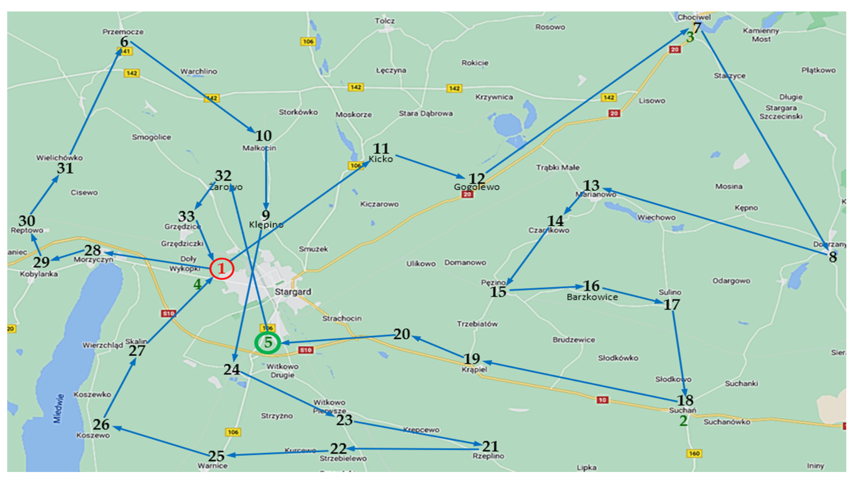
• Scenario 2: Each customer needs 121 kg of goods, so the demand vector z = (121, 121, …, 121)_{1 × 28}. The total demand of the customers equals: 28 × 121 = 3388, which is within the carrying capacity of two EVs.
• Scenario 3: Each customer’s demand is a random number from interval [100,1700]. Ten different demand vectors were generated. It was analysed how the sum of the customers’ demands affects the delivery plan.

After preliminary test calculations for different values of control parameters, it was assumed that satisfactory convergence of the evolutionary algorithm is achieved for:

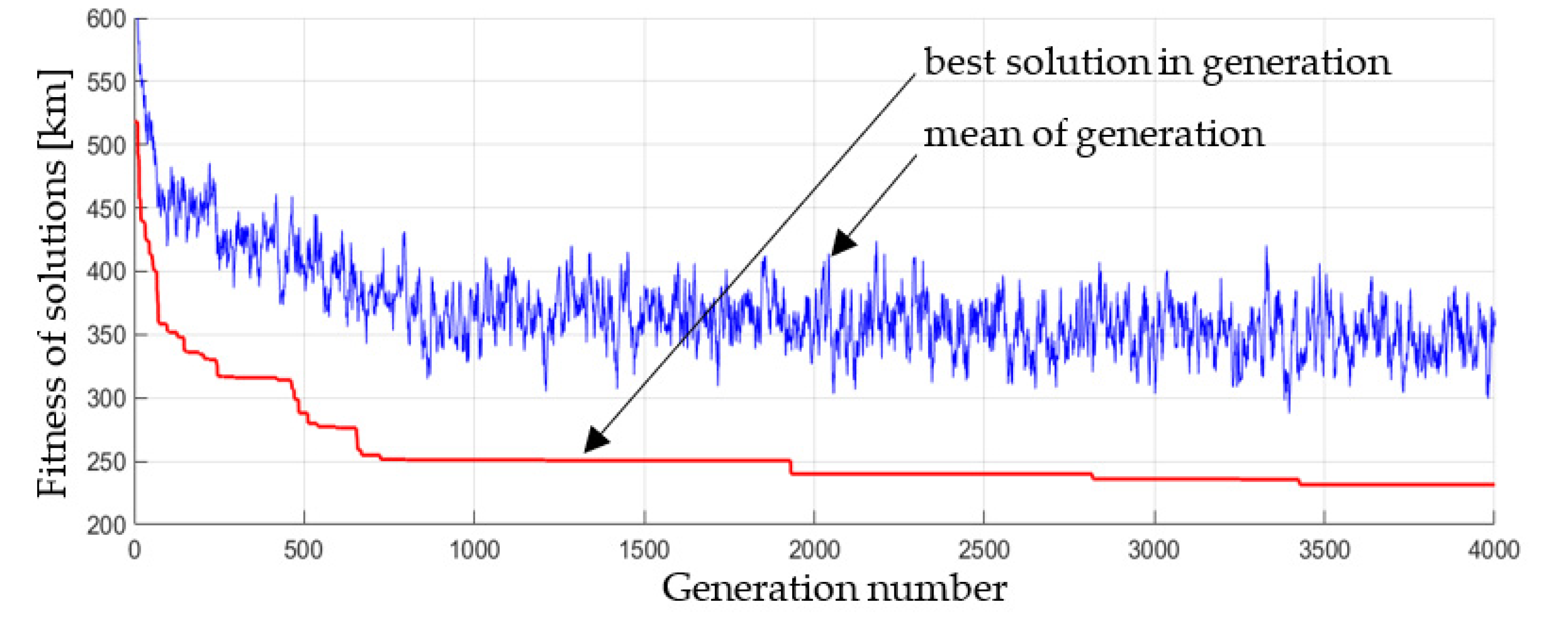
• Population size: G = 40;
• Number of elite individuals: E = 2;
• Mutation probability: P = 0.3;
• Number of populations: 20,000.

The computation time for the above parameters set is approximately 40 s.

Figure 5 shows the process of evolution for the first scenario. By using elite individuals, the best solution in each generation is preserved. It is represented by a red line that falls as better solutions are found. The figure also shows the average adaptation of individuals in each generation. This gives an idea of how much diversity of solutions is maintained by the mutation operator.

In solving the first scenario, the algorithm worked correctly and found a solution where one EV serves all the customers. During operation, it is necessary to charge the battery twice. In total, the vehicle covered a distance of 231.5 km. The best solution found is the following plan:

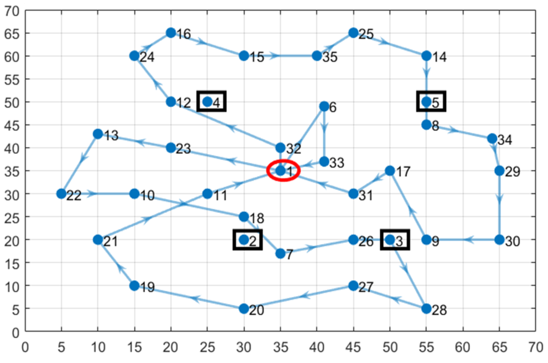
• Departure from the depot;
• Supplying the customers: 27, 26, 25, 22, 21, 23, 24, 11, 12, 7;
• Charging the battery in point 3 (Chociwel);
• Supplying the customers: 8, 13, 14, 15, 16, 17, 18, 19, 20, 32, 33;
• Charging the battery in point 4 (Shopping centre—Lipnik);
• Supplying the customers: 28, 29, 30, 31, 6, 10, 9;
• Return to the depot.

Figure 6 shows the order of the visited points on the map. The depot (1) and the visited charging stations (3 and 4) are highlighted. Charging stations 2 and 5 remain unused. The straight arrows between the points are symbolic. The vehicle is driven on real, much longer routes. It is worth noting that the route includes the three distinctive loops. After travelling to the southern loop, the vehicle heads to the north-eastern loop, where it charges the battery first. After travelling to the second loop, the battery is charged for the second time and the route is completed on the north-western loop.

For the second scenario, as expected, a plan for two EVs was obtained. The vehicles ‘shared’ the customers, so they had shorter routes to cover. One of the vehicles needs to replenish energy before returning to the depot. The evolutionary algorithm has found the following plan:

• Two EVs leave the depot;
• The first EV supplies the customers: 11, 12, 7, 8, 13, 14, 15, 16, 17, 18, 19, 20;
• The first EV charges the battery in point 5;
• The first EV supplies the customers: 32, 33;
• The second EV supplies the customers: 28, 29, 30, 31, 6, 10, 9, 24, 23, 21, 22, 25, 26, 27;
• Both EVs return to the depot.

The above plan requires the vehicles to cover 241.2 km, which is slightly more than in the first scenario. The visualization of the solution is shown in Figure 7.

During the implementation of the second adopted scenario, vehicle 1 mainly serves the eastern part of the region, while vehicle 2 initially travels north-west, then visits points south of Stargard.

The next stage of the study was to analyse the cases of randomly diversified customer demand. The number of vehicles needed to implement the plan depends on the total demand of all customers. For each sum, the minimum number of vehicles with a specific loading capacity can be specified—Table 1. For example, for the demand sum of 10,271, the result is 10,271/1700 ≈ 6.04, which means that at least seven vehicles are needed to deliver the ordered goods to all customers.

It is expected that the proposed algorithm for solving the E-VRP problem will be able to find delivery plans that require as few vehicles as possible. By comparing the number of vehicles required theoretically (

Table 2. The results obtained for scenario 3.

Random Problem No.	Demand Sum [kg]	Minimum Number of EVs	Solution Distance [km]	Used EVs
1	3358	2	304	2
2	7109	5	303	5
3	10,271	7	357	7
4	14990	9	454	10
5	19,992	12	542	13
6	22,814	14	611	15
7	37,251	22	891	28
8	14,475	9	428	9
9	15,155	9	432	10
10	15,589	10	446	10

, third column) with the number determined by the algorithm (Table 2, fifth column), it can be seen that in half of the cases, the algorithm found a solution with the minimum number of vehicles. In four cases, the solution includes one vehicle more than the minimum value (problem no. 4, 5, 6 and 9).

Problem number 7 is special. In this case, each customer demands more than 1000 kg of goods. As a result, a single vehicle can serve only one customer, even though it will not use all of its payload. Therefore, the algorithm correctly established the only possible plan which required 28 vehicles.

Figure 8 shows the solution to problem 2. The algorithm in this case found a plan that requires the minimum number of vehicles. Each vehicle travels a compact loop. Potential doubts can be raised by the inclusion of points 27 and 28 into the ‘red’ loop. However, it should be borne in mind that an important constraint is the quantities of goods ordered by the customers.

4. Assessment of the Performance of the Proposed Algorithm

The performance of the proposed coding method was assessed on the basis of two E-VRP instances described in [23]. The first example counts 25 points and the second one 35 points. In both cases, the point sets contain four charging stations. The order of point numbering has been changed to keep the numbering rule in the following order: base point, charging stations, customers.

To ensure the comparability of the obtained results, the maximum payload of the vehicle L_max = 200 and maximum reach of the vehicle R_max = 100 were adopted. The calculations were performed on the same computer as the example study in Section 3.

The proposed calculation algorithm based on permutation coding combined with evolutionary optimisation allowed obtaining the best solution of the first instance at the level of 247.4 km of the travelled route, which is the same result as obtained by Wang et al. [23]; however, the computation time was 4.8 s, which is slightly shorter than the Tabu search method and much better than the CPLEX method. In the solution of instance 1, customers are served by two vehicles. Each vehicle replenishes energy once during the tour.

Figure 9 shows the vehicle routes designated for the first instance. Point 1 is the depot and points 2–5 are the charging stations.

For the second of the examined cases, a much better solution was found than that published in [23]. Visiting all customers requires the use of three vehicles, two of which have to recharge energy during the tour. The third vehicle takes a short route visiting only two points. The total length of the route is 394.76 km. The calculations took 7 s. The solution is shown in Figure 10. The markings of the points are the same as in the first instance.

The results are compared in

Table 3. Comparison of the results obtained with the proposed method with the results published in the literature.

Method	Node Number	Result [km]	Time [s]	Reference
MILP encoding + Tabu search	20	247	5	[23]
	30	422.56	5
MILP encoding + CPLEX	20	247	49	[23]
	30	422.56	358
Permutation encoding + Evolutionary optimisation	20	247	4.8	proposed method
	30	394.76	7

. Two methods tested in [23] were referred to. Both are based on matrix coding, but differ in the method of solving the optimisation problem. On the basis of the obtained results, it can be concluded that permutation coding in combination with evolutionary optimisation has significant advantages and allows to quickly achieve solutions that are better than in other methods.

5. Discussion and Conclusions

The case study performed for north-western Poland concerned different scenarios of the demand for goods. The results allow us to observe that the developed evolutionary algorithm solves the defined E-VRP in a short time, generating formally correct and good results with respect to the adopted criterion. Of course, the evolutionary method does not guarantee finding the optimum, but the relatively low complexity of the example problem and visualisation of solutions on the map allow rating highly obtained solutions.

Figure 11 summarises the results for all tested scenarios. The impact of the uniform distribution of customer demand on the distance travelled by the vehicles. In particular, it illustrates the comparison of scenario 2 and the first random problem of scenario 3. Both cases are related to a similar total demand for goods, but the route determined for the random problem is 25% longer than for scenario 2. The uniform distribution of demand gives vehicles more freedom to choose their next customer. However, the great variation in demand may make it necessary for a vehicle to bypass certain customers and search for remote customers with a demand matching the volume of the carried cargo.

In addition to the case study, the algorithm performance was assessed in terms of computation time as well as its ability to find good solutions. For this purpose, the obtained times and quality of solutions were compared with the published results for two E-VRP instances. The conclusions from the comparison to other methods are promising. The proposed calculation algorithm is comparably fast and allows finding much better solutions.

The algorithm can be used to solve E-VRP-NL problems with the assumption that a critical point is identified for the function of battery charging time. This point sets the level, up to which vehicles are charged during a working day. Charging above this point takes too long and happens only during a long halt in the depot, for example at night. Therefore, the algorithm allows for the nonlinearity in a simplified manner, but this is in line with the practical operation of EVs by their drivers, who are forced to replenish energy within a limited time frame.

The model is restricted by the static distances between the landmark points on the map. The proposed method can be made more useful in practice by adding the time-of-travel criterion. In this way, the actual speed limits of vehicle traffic can be considered.

The implementation of the method in the dynamic fleet management system makes it possible to retrieve up-to-date data about disturbances related to increased traffic intensity and accidents on selected routes. Ongoing monitoring would allow for the method to be used for dynamic updating of the optimum vehicle route to avoid particularly congested sections. Extending the model to link it to the time axis is a planned direction for further research.

Depending on the needs of the users, the method can easily be extended to include the drop in the batteries’ capacity after a certain number of charging cycles. This is an issue that will begin to become more important during the next few years of the EVs’ operation.

The implementation of the method in practice may require additional experimental tests to be carried out on selected vehicle models to determine the energy consumption as a function of variable speed, load carried, and selected route.

In addition to ad hoc delivery planning, fleet management companies can use the proposed tool to simulate scenarios of fleet growth, diversification of vehicle size, driver hiring policies, diversification of delivery costs by customer location, etc.

The presented method can also be used as a tool to support investment decisions on the number and location of electric vehicle charging stations. Of course, such decisions must take into account not only the predicted needs of shipping and transportation companies but also the evolving market for passenger vehicles.

References

1. Ghorbani, E.; Alinaghian, M.; Gharehpetian, G.B.; Mohammadi, S.; Perboli, G. A Survey on Environmentally Friendly Vehicle Routing Problem and a Proposal of Its Classification. Sustainability 2020, 12, 9079. [Google Scholar] [CrossRef]
2. Wang, L.Y.; Song, Y.B. Multiple Charging Station Location-Routing Problem with Time Window of Electric Vehicle. J. Eng. Sci. Technol. Rev. 2015, 8, 190–201. [Google Scholar] [CrossRef]
3. Erdelić, T.; Carić, T. A Survey on the Electric Vehicle Routing Problem: Variants and Solution Approaches. J. Adv. Transp. 2019, 2019, 5075671. [Google Scholar] [CrossRef]
4. Erdoğan, S.; Miller-Hooks, E. A green vehicle routing problem. Transp. Res. Part E Logist. Transp. Rev. 2012, 48, 100–114. [Google Scholar] [CrossRef]
5. Montoya, A.; Guéret, C.; Mendoza, J.E.; Villegas, J. The electric vehicle routing problem with nonlinear charging function. Transp. Res. Part B Methodol. 2017, 103, 87–110. [Google Scholar] [CrossRef] [Green Version]
6. Kullman, N.; Goodson, J.; Mendoza, J.E. Electric Vehicle Routing with Public Charging Stations. Transp. Sci. 2021, 55, 3. [Google Scholar] [CrossRef]
7. Zuo, X.; Xiao, Y.; You, M.; Kaku, I.; Xu, Y. A new formulation of the electric vehicle routing problem with time windows considering concave nonlinear charging function. J. Clean. Prod. 2019, 236, 117687. [Google Scholar] [CrossRef]
8. Koç, Ç.; Jabali, O.; Mendoza, J.E.; Laporte, G. The electric vehicle routing problem with shared charging stations. Int. Trans. Oper. Res. 2019, 26, 1211–1243. [Google Scholar] [CrossRef]
9. Lee, C. An exact algorithm for the electric-vehicle routing problem with nonlinear charging time. J. Oper. Res. Soc. 2020, 1–24. [Google Scholar] [CrossRef]
10. Kancharla, S.R.; Ramadurai, G. Electric Vehicle Routing Problem with Non-Linear Charging and Load-Dependent Discharging. Expert Syst. Appl. 2020, 113714. [Google Scholar] [CrossRef]
11. Gheysens, F.; Golden, B.; Assad, A. A comparison of techniques for solving the fleet size and mix vehicle routing problem. OR Spektrum 1984, 6, 207–216. [Google Scholar] [CrossRef]
12. Bula, G.A.; Gonzalez, F.A.; Prodhon, C.; Afsar, H.M.; Velasco, N.M. Mixed Integer Linear Programming Model for Vehicle Routing Problem for Hazardous Materials. IFAC-PapersOnLine 2016, 49, 538–543. [Google Scholar] [CrossRef]
13. Madankumar, S.; Rajendran, C. A mixed integer linear programming model for the vehicle routing problem with simultaneous delivery and pickup by heterogeneous vehicles, and constrained by time windows. Sādhanā 2019, 44, 39. [Google Scholar] [CrossRef] [Green Version]
14. Xiang, X.; Tian, Y.; Zhang, X.; Xiao, J.; Jin, Y. A Pairwise Proximity Learning-Based Ant Colony Algorithm for Dynamic Vehicle Routing Problems. IEEE Trans. Intell. Transp. Syst. 2021. [Google Scholar] [CrossRef]
15. Shao, S.; Guan, W.; Ran, B.; He, Z.; Bi, J. Electric Vehicle Routing Problem with Charging Time and Variable Travel Time. Math. Probl. Eng. 2017, 2017, 5098183. [Google Scholar] [CrossRef] [Green Version]
16. Wang, L.; Gao, S.; Wang, K.; Li, T.; Li, L.; Chen, Z. Time-Dependent Electric Vehicle Routing Problem with Time Windows and Path Flexibility. J. Adv. Transp. 2020, 2020, 3030197. [Google Scholar] [CrossRef]
17. Froger, A.; Mendoza, J.E.; Jabali, O.; Laporte, G. Improved formulations and algorithmic components for the electric vehicle routing problem with nonlinear charging functions. Comput. Oper. Res. 2019, 104, 256–294. [Google Scholar] [CrossRef] [Green Version]
18. Flood, M.M. The Traveling-Salesman Problem. Oper. Res. 1956, 4, 61–75. [Google Scholar] [CrossRef]
19. Abdoun, O.; Abouchabaka, J. A Comparative Study of Adaptive Crossover Operators for Genetic Algorithms to Resolve the Traveling Salesman Problem. Int. J. Comp. App. 2011, 31, 49–57. [Google Scholar] [CrossRef]
20. Iwańkowicz, R.; Sekulski, Z. Solving of vehicle routing problem by evolutionary algorithm. Adv. Sci. Technol. Res. J. 2016, 10, 123–134. [Google Scholar] [CrossRef]
21. Malhotra, R.; Singh, N.; Singh, Y. Genetic Algorithms: Concepts, Design for Optimization of Process Controllers. Comput. Inf. Sci. 2011, 4. [Google Scholar] [CrossRef]
22. Chieng, H.H.; Wahid, N. A Performance Comparison of Genetic Algorithm’s Mutation Operators in n-Cities Open Loop Travelling Salesman Problem. In Recent Advances on Soft Computing and Data Mining; Springer: Berlin/Heidelberg, Germany, 2014. [Google Scholar] [CrossRef]
23. Wang, Q.; Peng, S.; Liu, S. Optimization of Electric Vehicle Routing Problem Using Tabu Search. In Proceedings of the 2020 Chinese Control and Decision Conference, Hefei, China, 22–24 August 2020. [Google Scholar] [CrossRef]
Figure 1. The structure of distance matrix D.
Energies 14 06651 g001
Figure 2. Solution decoding algorithm.
Energies 14 06651 g002
Figure 3. Example of E-VRP solution decoding.
Energies 14 06651 g003
Figure 4. Deployment of the depot (1), charging stations (2–5) and customers (6–33).
Energies 14 06651 g004
Figure 5. History of the evolution of the adaptation function during the optimization for the first scenario.
Energies 14 06651 g005
Figure 6. The visualization of the found solution for the first scenario.
Energies 14 06651 g006
Figure 7. The visualization of the found solution for the second scenario.
Energies 14 06651 g007
Figure 8. The visualization of the solution for problem 2 according to the third scenario.
Energies 14 06651 g008
Figure 9. Routes of the best solution (instance 1).
Energies 14 06651 g009
Figure 10. Routes of the best solution (instance 2).
Energies 14 06651 g010
Figure 11. The distance of the route depends on the total demand of customers.
Energies 14 06651 g011