MHD R&D Activities for Liquid Metal Blankets

Abstract

According to the most recently revised European design strategy for DEMO breeding blankets, mature concepts have been identified that require a reduced technological extrapolation towards DEMO and will be tested in ITER. In order to optimize and finalize the design of test blanket modules, a number of issues have to be better understood that are related to the magnetohydrodynamic (MHD) interactions of the liquid breeder with the strong magnetic field that confines the fusion plasma. The aim of the present paper is to describe the state of the art of the study of MHD effects coupled with other physical phenomena, such as tritium transport, corrosion and heat transfer. Both numerical and experimental approaches are discussed, as well as future requirements to achieve a reliable prediction of these processes in liquid metal blankets.

1. Introduction

As stated in the most recent European roadmap for a DEMO reactor [1,2], one of the candidate driver blankets that will be investigated in ITER is the Water Cooled Lead Lithium (WCLL) blanket concept. It uses water as a coolant at typical pressurized water reactor conditions (290–325 °C, 15.5 MPa) and lead lithium PbLi in eutectic composition as tritium breeder, neutron multiplier and tritium carrier. Other concepts, such as the Helium Cooled Lead Lithium (HCLL) and the Dual Coolant Lead Lithium (DCLL) blankets, are still being considered, in limited R&D activities, as potential long-term options.

In liquid metal (LM) blankets, the electrically conducting PbLi moves in the system under the action of the intense magnetic field that confines the fusion plasma.

It is well known that electromagnetic forces induced by the interaction of magnetic field and velocity significantly modify liquid metal flow behavior compared to hydrodynamic conditions [3]. The peculiar magnetohydrodynamic (MHD) flow distribution affects all phenomena that depend on the near-wall velocity profile, such as transport of tritium and corrosion products, and heat transfer. In addition, significant temperature gradients are present in breeding blankets, giving rise to buoyancy forces.

Recently, a review paper has been published aiming to identify the main MHD issues related to the design of liquid metal blankets and to present the state of the art of the study of some fundamental MHD phenomena that occur in these complex systems [4]. In the present paper, we want to provide a complementary description of multiphysics MHD phenomena, focusing on recent progress and fusion-relevant applications. For instance, tritium transport and corrosion in hydrodynamic LM systems have been studied extensively for different cases and operating conditions. However, those processes in MHD flows have been investigated only in a few publications. Since transport processes depend on the velocity distribution, the MHD flow that results from the interaction of the moving LM with the external magnetic field has to be used as input for their analysis. Features to be taken into account are, e.g., increased velocity at electrically conducting walls aligned with the magnetic field, turbulence anisotropy, reversed flows caused by magneto-convection and electromagnetic coupling.

Models have been proposed to integrate into the analysis of MHD flows corrosion and tritium transfer across material interfaces, permeation through structural materials and into the coolant. In order to identify the fundamental steps for a long-term strategy aimed at implementing and validating accurate and robust modeling tools for application to fusion technology, it is first required to outline the actual state of the art of the different R&D topics. Therefore, a review of modelling approaches, validation experiments and future requirements for analyses of coupled MHD phenomena is presented in this paper. Another important step towards a better understanding of multiphysics MHD flows in complex systems is the development of system codes. The main features, advantages and limitations of these predictive tools are discussed as well.

2. Problem Description

We consider in the following the general equations governing the magneto-convective flow of an electrically conducting fluid in a magnetic field B. They describe the conservation of momentum and mass:

$$\rho \left(\frac{\partial \mathit{v}}{\partial t}+\left(\mathit{v}\cdot \nabla \right)\mathit{v}\right)=-\nabla p+\rho \nu {\nabla }^2\mathit{v}-\rho \beta \left(T-T_0\right)\mathit{g}+\mathit{j}\times \mathit{B},\nabla \cdot \mathit{v}=0,$$

(1)

where v denotes the velocity, p is the deviation of pressure from isothermal hydrostatic conditions at the reference temperature T₀, $\mathit{g}$ stands for gravitational acceleration, and $\mathit{j}\times \mathit{B}$ is the electromagnetic Lorentz force induced by the interaction of imposed magnetic field B and electric current density j. The latter is determined via Ohm’s law $\mathit{j}=\sigma \left(-\nabla \varphi +\mathit{v}\times \mathit{B}\right)$ that, combined with the condition for charge conservation, $\nabla \cdot \mathit{j}=0$, results in a Poisson equation for the electric potential $\varphi$:

$$\nabla \cdot \nabla \varphi =\nabla \cdot \left(\mathit{v}\times \mathit{B}\right).$$

(2)

Density changes due to temperature variations in the liquid metal are described by the Boussinesq approximation. The physical properties of the fluid, density ρ, kinematic viscosity ν, volumetric thermal expansion coefficient β, and electric conductivity σ are taken at the reference temperature T₀.

The temperature distribution in the fluid is given by the energy balance equation

$$\rho c_p\left(\frac{\partial T}{\partial t}+\left(\mathit{v}\cdot \nabla \right)T\right)=k{\nabla }^{2}T+Q$$

(3)

where c_p is the specific heat of the fluid at constant pressure, k the thermal conductivity and Q a volumetric thermal source.

The flow can be characterized by three dimensionless groups, the Hartmann number $Ha$, the Reynolds number $Re$ and the Grashof number $Gr$,

$$Ha=LB\sqrt{\frac{\sigma }{\rho \nu }},\hspace{1em}Re=\frac{u_{0}L}{\nu },\hspace{1em}Gr=\frac{g\beta L^3\Delta T}{{\nu }^2}.$$

(4)

The former one gives a nondimensional measure for the strength B of the imposed magnetic field and its square quantifies the ratio between electromagnetic and viscous forces. The second expresses the ratio of inertia to viscous forces. Alternatively, the interaction parameter $N=H{a}^2/Re$ can be used to weigh the relative importance of electromagnetic and inertia forces. The Grashof number characterizes the intensity of buoyancy. The quantities L and u₀ are a typical size and mean velocity in the considered geometry. A characteristic temperature difference ΔT can be defined for instance through the volumetric heat as ΔT = QL²/k.

Equations (1)–(3) are solved in the fluid and Equations (2) and (3) also in electrically and thermally conducting solid structures, by applying appropriate boundary conditions. The fluid velocity vanishes at walls (no-slip condition) and continuity of wall-normal currents and electric potential is assumed at interfaces (perfect electrical contact between fluid and solid material). At external surfaces towards an electrically insulating environment, wall-normal currents vanish. At the entrance to the computational domain, the flow is prescribed and often assumed as being fully developed, while at the exit an advective outflow condition can be applied.

3. Theoretical Description of MHD Flows

The design of test blanket modules (TBMs) for ITER and breeding blankets for DEMO requires accurate and reliable predictive tools. Depending on the application, the type of information required, and the level of detail, different methods can be employed to study theoretically MHD flows under fusion-relevant conditions.

In the following, we discuss the advantages, limitations, development progress, and application examples of various approaches, such as Computational Fluid Dynamics (CFD) simulations, asymptotic analysis and system codes.

3.1. Numerical Simulations

CFD codes provide a detailed description of flow features, since the domain discretization is highly refined. Moreover, they may be used to simulate turbulent flows, heat transfer and other coupled MHD phenomena.

Preliminary numerical simulations prior to the start of an experimental campaign can serve to determine which system’s parameters need the highest measurement accuracy. This type of information is very useful during the experiment’s conceptual phase, since it helps to select the type of sensors based on their accuracy when recording the desired quantity and hence it increases the consistency of experimental and numerical results. Simulations can provide indications for a suitable arrangement and for the needed number of sensors in specific zones of interest in the system. Numerical simulations can also be used to analyze the sensitivity of a model to the variation of given parameters.

The simplicity of the electromagnetic part of the governing Equations (1)–(3) can be misleading. In fact, accurate numerical simulation of flows at blanket-relevant high values of Ha is a computationally challenging task, significantly more than in the case of hydrodynamic flows at the same Re and Gr. The key reason is the numerical stiffness of the problem, which manifests itself as thin boundary and internal shear layers and the very large ratio between the largest and smallest typical time and length scales (see Section 3.4 as well as [3,5] for a more detailed discussion). One significant consequence of the stiffness is that high-Ha flows, especially those with unsteady behavior, are not directly amenable to analysis by general-purpose CFD codes based on finite-volume or finite-element discretization on unstructured grids. A review of numerical methods and outstanding questions can be found, e.g., in [3].

Another important factor in analyses of unsteady flows is the availability of effective, accurate and well parallelizable solvers for elliptic equations. A time steep in a numerical solution of the system (1)–(3) inevitably requires solving two such equations, one for electric potential (2) and one for pressure (here we assume that a projection method is used to satisfy incompressibility). The typically very small Prandtl number, $Pr=\rho \nu c_p$/$k$, of liquid metals means that the heat conduction term in the energy Equation (3) has to be treated implicitly in order to avoid severe limitations on the size of the time step, so another elliptic equation for temperature must be solved. Implicit treatment of viscous terms in (1) is also often applied, which implies another three elliptic equations for velocity components. It is not uncommon that over 90% of the computational time in an analysis of an unsteady high-Ha flow is spent on the solution of elliptic equations. High-performance computing based on massive parallelization becomes necessary in many cases (see, e.g., [6]).

In recent years, considerable advances have been made in the numerical prediction of coupled MHD-heat transfer phenomena in complex blanket-relevant geometries and under fusion conditions [7,8]. However, even when relatively small computational domains are considered, large computing resources are needed, which results in long simulation time. The latter can be reduced by introducing some assumptions in the flow modelling, as described in the following section for the asymptotic numerical approach.

3.2. Asymptotic Analysis

While the study of MHD flows under very strong magnetic fields represents a considerable challenge for numerical simulations, asymptotic analyses benefit from flow conditions that are typical for fusion applications. From a mathematical point of view, steady-state flows in strong magnetic fields constitute a singular perturbation problem. One may neglect inertia and viscous forces in comparison with the strong Lorentz and pressure forces (which largely balance each other) in the core of the flow domain if $N\to \infty$ and $Ha\gg 1$. Viscous effects at walls can be taken into account by a boundary layer analysis, which allows satisfying the no-slip condition at fluid–solid interfaces. Asymptotic analyses can be used to study fully developed flows in long straight pipes and ducts (see, e.g., [9,10]). However, the method has been also applied to some 3D flows such as those in ducts with variable cross-section [11] or in non-uniform magnetic fields [12]. For the latter case a good agreement with experiments has been achieved for $Ha\gg 1$.

The initial idea of an asymptotic description of general 3D flows, which dates back to Kulikovskii [13], has been reformulated in tensor notation, extended by a boundary layer analysis, and developed to treat walls of arbitrary electric conductivity [14]. The latter approach takes advantage of the fact that variations of all flow quantities along magnetic field lines are analytically known, which allows for a kind of “projection” of the 3D problem onto the duct walls, where the remaining 2D equations for pressure and electric potential are numerically solved using boundary-fitted coordinates. In a final step, the entire 3D flow is reconstructed by analytical means. The method allows for fast computations (seconds to minutes) on standard PCs, even for relatively complex geometries. On very coarse grids, one already achieves a good approximation of flow quantities, as shown by the example of a 3D flow in a fringing magnetic field displayed in Figure 1. The validity of the method has been verified by comparison with analytical solutions, full 3D simulations, and experiment [12,15]. The general formulation of the code allows calculations for quite complex domains, as illustrated by the examples in Figure 2, which shows the entrance and exit flows of a DCLL blanket sector, or in a model geometry of a DCLL blanket module.

While asymptotic methods give accurate results with almost negligible numerical effort, they are unable to predict the influence of inertia on MHD flows. Even if the core flow remains almost inertialess for $N\gg 1$, inertia at sharp corners or in high-velocity boundary layers may lead to local flow separation or instabilities that cannot be predicted by the latter method. If such phenomena are expected to occur, one has to perform full 3D time-dependent numerical simulations.

3.3. System Codes

System thermal-hydraulics (SYS-TH) codes are a class of numerical tools developed since the 1970s in the framework of nuclear reactor safety technology for fission reactors [18]. SYS-TH codes aim to represent with sufficient accuracy all the main phenomena occurring in a nuclear reactor during operational and accidental transients and, as such, are used to perform deterministic safety analyses for licensing purposes. A SYS-TH model is created through a process called “nodalization” that subdivides the reactor into control volumes in which a set of linearized algebraic equations, derived by variants of the finite volume and difference methods, are solved to obtain the distribution of physical properties (temperature, velocity, pressure, etc.) in a set of nodes. The key features of SYS-TH codes are the quite coarse spatial resolution and the reliance on closure laws derived empirically to model complex phenomena. Modelling choices are available to represent reactor components with an increasing level of fidelity from lumped (0D) or 1D modules to simulate flow in primary and secondary loops, up to fully 3D to recreate the phenomena occurring in the reactor core. Notable examples of SYS-TH codes are, among others, RELAP5, TRAC/TRACE, ATHLET and CATHARE.

SYS-TH codes are often described as multiphysics, best-estimate, safety and industrial computational tools [18]:

• Multiphysics: to include all relevant phenomena encountered in a nuclear reactor from two-phase thermal-hydraulics to neutron kinetics diffusion equations and fuel thermomechanics.
• Best-estimate: to provide an accurate prediction of selected figures of merit and to be as close as possible to the physical reality that one aims to simulate.
• Safety: suitable to demonstrate the reactor safety for licensing purposes, namely developed according to a clearly defined quality assurance (QA) methodology, accompanied by uncertainty quantification (UQ), extensively verified and validated to prove the code scalability.
• Industrial: i.e., robust and computationally inexpensive to allow simulations on a wide test matrix for sensitivity analysis and UQ in a reasonable timeframe.

In the past two decades, SYS-TH codes have been further developed to make them able to represent dominant characteristic phenomena in fast breeder reactors (FBR) and other innovative Generation IV fission reactor concepts [19]. The development of a DEMO design has also motivated lines of research aimed at improving the capability of SYS-TH codes to deal with fusion reactor environment for both liquid metal and solid breeder blankets [20,21]. Despite the progress achieved, SYS-TH codes for fusion applications are still far from an acceptable maturity. In particular, the prediction of MHD effects in liquid metal blanket systems is still very challenging due to the limited availability of closure laws to describe them [22,23]. This is in stark contrast with the advancements made in recent years in the field of CFD analysis, where both commercial and open-source codes are nowadays able to simulate liquid metal MHD flows at reactor-relevant magnetic field intensity and at blanket scale [24].

Relying on closure laws to ensure accurate representation of physical reality is not necessarily associated with a lack of accuracy, and, in fact, the experience of the nuclear industry has clearly demonstrated that SYS-TH codes can provide reliable results for reactor safety and design if closure laws of sufficient quality are available [18]. The possibility of performing system-scale coupled thermal-hydraulics/MHD analyses at largely reduced computational cost is attractive for performing sensitivity and uncertainty analyses even when mature CFD codes for fusion modelling are available. The critical point is to develop closure laws for MHD effects, such as MHD pressure drop, electromagnetic coupling and heat transfer, based on current knowledge, as discussed in the next section, and to define future R&D steps for their improvement.

3.3.1. MHD Pressure Loss, Electromagnetic Coupling and Heat Transfer

Among the various MHD effects that influence liquid metal blanket performance, pressure losses and modified heat transfer coefficients are often considered the most critical ones [25]. Therefore, it is reasonable that they should be prioritized for implementation in SYS-TH codes.

Regarding MHD pressure losses, SYS-TH codes must be able to predict distributed (2D) and concentrated (3D) losses and how they are impacted by electromagnetic coupling, buoyancy and Q2D turbulence. Pressure losses in fully developed flows at fusion-relevant parameters are well characterized by theoretical and experimental works and scaling laws are available for both circular pipes and rectangular ducts [4,26,27].

The prediction of 3D MHD losses is more demanding due to the wider range of governing parameters involved and the need to take into account the effects of inertia and viscous forces. Moreover, they are caused by many scenarios, such as the presence of fringing magnetic fields of general orientation, discontinuous wall conductivity, and complex geometry (bends, cross-section variation, etc.) [26]. Therefore, it is difficult to develop a scaling law that has universal validity. The needed coefficients have to be chosen by experienced analysts, from detailed numerical simulations or dedicated experiments in representative and specific conditions. A recent review of theoretical and experimental works on 3D MHD losses may be found in [4].

While 2D and many 3D phenomena in MHD duct flows are reasonably well understood and ready for implementation in SYS-TH codes by adaption of friction factors, other phenomena that do not occur in hydrodynamic flows make their implementation in SYS-TH codes challenging. One example is the electromagnetic coupling caused by leakage currents between parallel channels that share electrically conductive walls. Its effect depends on the number of coupled channels, their orientation with respect to the magnetic field, the conductivity of the walls, etc. [4]. Analytical solutions exist only for very special electrical boundary conditions [28] so that for applications in complex blanket geometries only coupled 2D or 3D simulations can provide the relevant friction coefficients when general scaling laws do not exist [29,30,31]. The problem becomes even more complex for flows in multiple coupled bends, where the coupling can be responsible for strongly increased flow in external ducts, while the flow in the central channels is significantly reduced, as predicted by Madarame et al. [32] and shown in experiments by Stieglitz et al. [33].

Another phenomenon that is difficult to implement in SYS-TH codes is the buoyancy force that aid or hamper the forced flow circulation if directed upward or downward, respectively [26]. While it is straightforward to take changes of cross-section averaged density into account in modified correlations for friction coefficients, strong temperature gradients across channels may lead to flow separation and the formation of vortices (preferentially Q2D in strong magnetic fields) with unexpected impact on pressure distribution and heat transfer [34].

The development of closure laws for heat transfer modelling in liquid metals is still a topic under active research for advanced SYS-TH codes for fusion reactor applications. Since these fluids are characterized by a small Prandtl number, $Pr$ $\ll$ 1, the Nusselt number, Nu, cannot be predicted by correlations originally developed for air and water. For forced convection, we have in general Nu = Nu(Pe, Pr), where $Pe=\rho u_0{c}_{p}L/k$ is the Peclet number [35]. For applications in fusion blankets, in which the flow is subject to strong magnetic fields, heat transfer in terms of the Nusselt number depends in addition on MHD parameters, Nu = Nu(Pe, Pr, Ha, N). For N $\gg 1$ and Ha $\gg$ 1, the magnetic field is expected to dampen velocity oscillations in the flow and revert it to a laminar state, thus degrading the heat transfer [27,36]. Nevertheless, experiments have demonstrated that MHD velocity profiles can promote a higher heat transfer than hydrodynamic flows. This is partially attributable to thin MHD boundary layers. Likewise important are the high-amplitude large-scale flow structures (vortices and jets) that develop in flows with intense magnetic field and other strong forcing. Such structures often significantly increase rates of mixing and local heat transfer (see the recent review [5] and references therein). An important example of this general phenomenon is flow in ducts with electrically conducting walls, where high-velocity jets at the sidewalls may become unstable and locally enhance the heat transfer [37,38]. Heat transfer in turbulent pipe flow at moderate Hartmann numbers has been studied in [39] and summarized in a correlation Nu(Pe, Ha). Despite these findings, the knowledge accrued has yet to be consolidated in scaling laws that can be then implemented in SYS-TH codes.

3.3.2. State-of-the-Art of MHD Modelling in SYS-TH Codes

To the best of our knowledge, there are five SYS-TH codes that feature some MHD modelling capabilities for liquid metal blanket systems: RELAP5 [40], MARS-FR [41], MELCOR [42], MHD-SYS [43] and GETTHEM [44]. They are listed in

Table 1. SYS-TH capabilities for MHD modelling.

Code	2D Loss	3D Loss	Coupling	Heat Transfer
RELAP5-3D [40]	Yes	Only for fringing magnetic field	No	No
RELAP5/MOD3.3 [23]	Yes	Yes	No	No
MARS-FR [45]	Yes	No	No	No
MELCOR 1.8.5/1.8.6 [46]	Yes	No	No	No
MHD-SYS [43]	Yes	Estimated through coupling	Based on analytical relations	Based on analytical relations
GETTHEM [47]	Yes	Yes	No	No

with regard to their capacity to predict MHD pressure losses, electromagnetic coupling, and heat transfer. RELAP5-3D is the only code that provides MHD modelling capabilities out-of-the-box, whereas all the others have been modified with custom models for this purpose. MHD-SYS has been developed specifically to simulate MHD effects.

Prediction of MHD pressure losses for fully developed flows (2D loss) is implemented in all the codes with a similar approach, i.e., the modification of the friction loss coefficient. Different implementations are instead adopted for 3D losses, and it should be highlighted that no SYS-TH code is currently able to cover all the scenarios that can cause these additional pressure drops. MARS-FR and MELCOR do not provide any support for this feature, whereas RELAP5-3D uses an ad hoc treatment only for the special case of a fringing magnetic field. MHD-SYS is unable to directly calculate 3D losses, but it supplies boundary conditions to a coupled CFD tool (the mhdFoam solver of OpenFOAM) to estimate them. A more general modelling of 3D losses is used by RELAP5/MOD3.3 that supports the automatic calculation of 3D loss coefficients through the specification of geometrical parameters in reserved words within the input deck, e.g., due to the presence of bends, cross-section variation and discontinuous electrical insulation. GETTHEM follows a similar approach for bends, whereas cross-section changes are represented with a fixed loss coefficient. No support is provided for insulation discontinuities, while a preliminary model for pressure penalty due to obstacles is available.

Electromagnetic coupling and heat transfer modelling are features present only in MHD-SYS. The used models rely exclusively on analytical solutions for very special combinations of wall conductivity and orientation of the magnetic field so that their generalization to blanket relevant applications is not possible.

3.3.3. A Validation Exercise for SYS-TH Code MHD Modelling: HCLL TBM Mock-Up

To illustrate the capability of a SYS-TH code including MHD effects, the custom module for RELAP5/MOD3.3 developed at Sapienza University of Rome is used to reproduce pressure distribution measured in a scaled mock-up of a HCLL TBM [48]. The experimental campaign predicts the global isothermal flow distribution in the considered blanket concept. This experimental data can be regarded as a good approximation of an integral effect test (IET) to validate the developed module. A full description of the validation exercise and the models implemented can be found in [23].

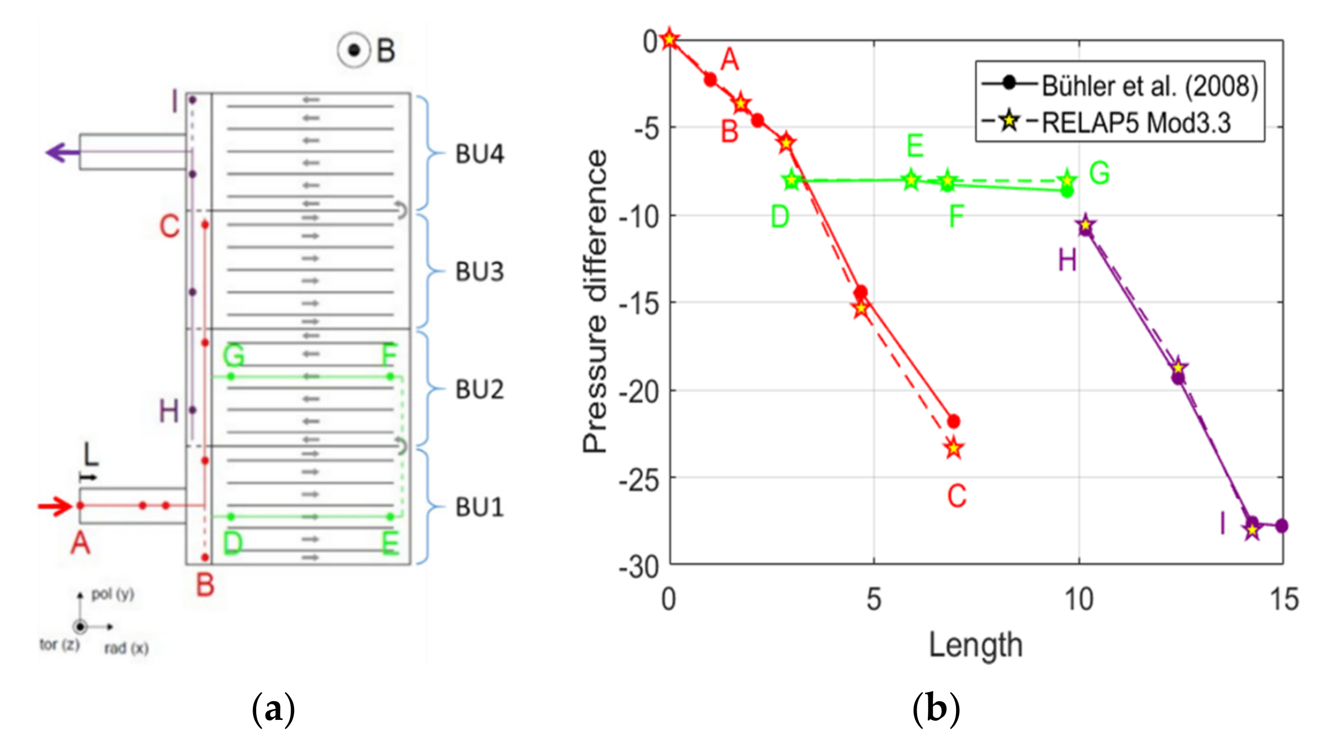
Figure 3a depicts a poloidal–radial view of the mock-up, pressure taps (A–E), and the liquid metal (NaK) flow path: feeding pipe (A), inlet manifold (B,C), inflow in BU1 (D,E) and outflow in BU2 (F,G), outlet manifold (H,I). The liquid metal flow path consists of numerous bends and cross-section variations, which introduce significant 3D MHD pressure losses, and features electromagnetic coupling of neighboring fluid domains, since the walls are electrically conducting.

In Figure 3b, the comparison between the experimental and RELAP5/MOD3.3 results for nondimensional pressure drop is shown for Ha = 3000 and Re = 3360. As scaling parameters we choose the toroidal half-length of a BU, L = 0.045 m, and the pressure scale p₀ = σu₀LB². The reference pressure value is imposed at location A. The code shows an excellent agreement with the experimental data in terms of total pressure loss and local values (−1% < ε < +14%), even without a model to represent electromagnetic coupling. The latter does not affect the overall pressure loss estimate due to the low contribution from BUs. On the contrary, the system code is not able to reproduce the flow distribution in the BUs, since it is significantly influenced by coupling [49]. Further model development is required to provide accurate predictions of flow distribution in Bus, in particular when heat transfer has to be quantified.

3.4. Requirements for Theoretical Analysis under Fusion Conditions

Common to all analysis methods discussed in Section 3, is the need for a database containing experimental data for validation of implemented models. Some of the experimental results that can be used for such a purpose are discussed in Section 4.

Various types of benchmark experiments have to be planned depending on validation purposes, e.g., tests to validate specific models or to improve the accuracy of parameters that are required for calculations. Both single effect and integrated multiple effect experiments have to be foreseen. The latter ones are also referred to as mock-up experiments. They include all essential features of a blanket concept with the aim to improve and finalize the design.

In the following section, we present some of the requirements for a proper theoretical investigation of fusion-relevant problems both by means of CFD and by using system codes.

3.4.1. Grid Generation

One of the most challenging aspects of numerical simulation of MHD flows in a strong magnetic field is the resolution of very thin boundary and internal layers, which form along walls and in the fluid at electrical or geometrical discontinuities of the wall. In order to properly resolve these layers, a minimum number of grid points is required [3]. For this purpose, non-uniform meshes that are coarser in the core regions and refined towards the layers have to be employed. MHD boundary layers are best resolved by using a prism layer. In general, structured grids, i.e., orthogonal and with non-skewed cells, lead to better performance. However, when studying MHD flows in complex geometries related to fusion blankets, hybrid unstructured meshes seem more suitable to meet the resolution requirements without excessive computational costs. This type of grid has some advantages compared to structured meshes, since it facilitates re-meshing and local refinement due to the possibility of clustering nodes in selected zones. For the study of MHD flows in complex geometries, as present in fusion reactors, the meshing tool should allow an automatic generation of the computational grid starting from a CAD model and permit effective control of local refinement in shear layers and regions of interest. In Section 3.4.2 an example of the influence of grid topology on the accuracy of the solution is discussed.

An option to be taken into account is the use of an adaptive mesh refinement (AMR) technique to adjust the accuracy of the solution within certain sensitive regions of the simulation domain by refining the mesh during runtime dynamically and locally according to given criteria [50].

Due to the very large number of nodes expected to be required to discretize a blanket related geometry, high-performance parallel computing is essential to reduce the computational time. However, simulation of MHD flows in an intense magnetic field, coupled with mass and heat transport phenomena, in realistic blanket models, remains a challenging time- and resource-consuming procedure.

3.4.2. Numerical Schemes

When simulating MHD flows at large Hartmann numbers, there exists a strong dependency of numerical errors in the solution on the grid topology. If unstructured meshes are used, discretization corrections are required, which account for non-orthogonality and skewness of the cells. A significant source of error can also originate from the numerical diffusion that arises from the truncation error. By using second-order discretization schemes and mesh refinement, the effects of numerical diffusion on the solution are reduced.

Discretization schemes with good conservation properties (conservation of mass, momentum, internal and kinetic energy, and, critically, electric charge) appear to be a preferable choice for flows at high Ha [6,7,8]. For instance, Ni et al. [51,52] developed an algorithm, which retains the conservative properties of the current density field, by using a proper interpolation procedure of current fluxes from cell-faces to cell-centers. Numerical errors can also derive from the computation of the electric current via Ohm’s law in flow regions where j is very small. This is because the two terms $\nabla \varphi$ and $\mathit{v}\times \mathit{B}$ are of nearly the same magnitude but with opposite signs. The computation of gradients of electric potential requires appropriate numerical schemes, such as Least-Squares (LS) or skew-corrected Green–Gauss (GG_corr) [53].

As an example to show the influence of grid topology on the prediction of MHD flows and the need for suitable corrections for the discretization of the potential gradient when using unstructured meshes, the MHD flow in an electrically insulating pipe at Ha = 1000 has been calculated. Two types of grids have been considered. The former one represents a block-structured mesh, a so-called O-grid, which consists of a central square block surrounded by four blocks that adapt to the curved pipe wall (see Figure 4a). The grid corners of the inner block, highlighted by red circles, represent discontinuities in the mesh structure that can introduce numerical errors in the solution. The second mesh, created by using the software STAR-CCM+, consists of polygonal cells in the duct cross-section (Figure 4b). In both grids, boundary layers are resolved by hexahedral elements with adequate grading in wall-normal direction. In Figure 4 only the core grid is visualized.

Simulations have been performed by changing the discretization scheme used for the calculation of the electric potential gradient. The results displayed in red in Figure 4 have been obtained by using the Green–Gauss scheme without skewness correction (GG_uncorr), the blue curve by Green–Gauss combined with a linear interpolation for the correction (GG_corr), and the green profile by a least square (LS) scheme. For insulating walls, the determination of the electric potential gradient by means of GG_uncorr introduces an error whose magnitude depends on the mesh topology, and this scheme is very sensitive to grid irregularities. Applying either corrected GG_corr or LS for the electric potential gradient leads to a significant improvement of the solution. Skewness-related perturbations are minimized so that errors are caused mainly by the grid cell size and not by the mesh type. However, for very large Ha (fusion conditions) the most accurate results for MHD flow in circular pipe have been obtained by using a grid with a structured core, a layer of hexahedral elements to resolve the boundary layers, and an unstructured mesh to connect both of them, together with LS scheme for electric potential gradient discretization [56].

3.4.3. Suitable Closing Laws for SYS-TH Codes

In SYS-TH codes the main issue is the absence of closure laws able to describe the effects of electromagnetic coupling and MHD velocity modifications which affect heat and mass transfer. In addition, the coefficients to be used for scaling laws to estimate 3D MHD losses have to be determined. Experimental and numerical data available in the literature must be expanded for these purposes. On the same note, it is challenging to demonstrate the code’s scalability since no past experimental work qualifies as IET and among planned ones, only the ITER campaign will satisfy all requirements (cf. Section 4 and [57]). Therefore, it would be highly desirable to plan separate effect tests to obtain experimental data for the development of SYS-TH models, which can be integrated with numerical activities performed with validated CFD tools. Moreover, there is the need for at least one IET to provide support for SYS-TH code validation before the experimental campaigns in ITER.

4. Experiments

Despite the great progress of computational tools, made possible by the increased availability of high-performance computing, numerical codes are not yet able to simulate all types of 3D MHD flows at fusion-relevant parameters in blanket geometries with enough reliability and accuracy. Empirical research remains, therefore, the principal method for advancing the knowledge of complex blanket flows, and experiments are necessary for the validation of computational tools.

MHD flow in an outboard blanket module in ITER for a typical magnetic field B = 4 T, length L = 0.1 m, u₀ = 0.1 m/s and for PbLi properties as shown in

Table 2. Thermophysical properties of PbLi at 400 °C and examples of possible model fluids that allow experimentation at room temperature. Nondimensional parameters have been evaluated for experimental conditions with B_exp = 2 T, L_exp = 0.05 m and u₀ = 0.1 m/s. For the Grashof number Gr a wall heat flux of 10 W/cm² is assumed.

	ρ kg/m3	ν × 106 m2/s	σ × 10−6 1/Ω/m	k W/m/K	β × 103 1/K	Re	Ha	Gr
PbLi 400 °C	9719	0.161	0.849	22.4	0.122	29,585	2273	1.2 × 109
Hg 20 °C	13,546	0.115	1.04	8.72	0.181	43,478	2584	9.6 × 109
GaInSn 20 °C	6353	0.340	3.32	24	0.122	14,706	3920	2.7 × 108
NaK 20 °C	868	1.06	2.87	21.8	0.29	4717	5585	7.3 × 107

, is characterized by a Hartmann number close to Ha = 9000. Experimental reproduction of such numbers is challenging for several reasons. In laboratory experiments, the strength of the magnetic field is limited to about B_exp $\lesssim$ 2 T when normal conducting copper magnets are used. Moreover, the available space in the magnets reduces the typical length scale for mock-up experiments by at least a factor of two (see, e.g., [58]), i.e., L_exp $\lesssim$ 0.05 m. If thermal insulation is required, L_exp could become even smaller. Therefore, Hartmann numbers in PbLi mock-up experiments are limited to Ha < 1000–2000. Higher values of Ha are possible only in superconducting solenoids, where, however, the length of channels with transverse magnetic field is limited by the size of the magnet bore [59]. In addition to this, MHD experiments with PbLi have to be performed at high temperatures. This results in thermoelectric disturbances of signals of the measured induced electric potential and difficulties in operating the flow meters and pressure transducers.

Given the problems associated with the high-temperature operation of PbLi loops, one may consider using model fluids, such as mercury, Hg [60], alloys such as gallium indium tin, GaInSn [61,62], or sodium potassium, NaK [63,64,65], which allow for MHD experiments at room temperature. As shown in Table 2, Hg is a preferred choice for studying mixed magneto-convection since its usage leads to Gr values one or two orders of magnitude higher than other liquid metals in the same conditions. The highest Hartmann numbers may be reached by using NaK. The drawback of using Hg is toxicity and for NaK is its chemical reactivity with oxygen or water, so that special precautions are required during preparation and conduction of experiments. NaK has the advantage that good electrical contact between fluid and wall is established after wetting, and corrosion issues do not exist in the temperature range of operation. Reasonable Hartmann numbers can be reached also with GaInSn, but electrical contact at the interfaces suffers from poor wetting capability. This requires special manual treatment of all surfaces exposed to the alloy in MHD experiments, since contact resistance by residual oxide layers influences the flow behavior in terms of pressure drop, velocity and potential distribution [66].

MHD experiments with model fluids fall into two major categories: fundamental or applied research. The first group includes experiments in generic geometries such as pipes, ducts, expansions and bends, for investigations of stability of laminar flows, transition to turbulence, heat transfer and buoyant flows. The results from these experiments constitute a valuable database for the validation of numerical tools [3,4].

The other type of experiment aims at demonstrating the feasibility of technological aspects, such as a reduction in pressure drop by electrically insulating coatings or flow channel inserts [67,68], or at studying complex electrically coupled MHD flows in scaled mock-ups of entire blanket modules.

Before discussing some examples of MHD experiments, it is worth mentioning a few aspects concerning measuring techniques for MHD flows at high Hartmann numbers.

Measurements of flow rate, pressure differences, and electric potential are straightforward, at least for model fluids. In experiments performed, e.g., in the MEKKA facility at KIT [64], it is possible to determine flow rates up to 25 m³/h, differential pressure between 30 pressure taps, and distribution of potential by up to 600 sensors on the wall or at the fluid–wall interface. The latter ones are of particular importance, since for $Ha\gg 1$, potential is constant along magnetic field lines and hence, the wall data give a good picture of the values inside the core of the fluid. Moreover, it is possible to calculate from Ohm’s law the components of velocity in the plane perpendicular to the magnetic field according to

$${\mathit{v}}_{\perp }=\frac{1}{B^2}\left(-\nabla \varphi \times \mathit{B}\underset{\approx 0}{\underbrace{-\frac{\nabla p}{\sigma }}}\right),$$

where for flows in insulating or thin-wall ducts, the current density (or pressure gradient) is negligible compared to potential gradients. Therefore, the potential $\varphi$ may be interpreted as an approximate stream function of the flow and we can determine the velocity field from wall potential measurements, i.e., $u\approx B^{-1}\partial \varphi /\partial z$ and $w\approx -B^{-1}\partial \varphi /\partial x$. As an example, Figure 5 shows the distribution of axial velocity determined from wall potential measurements in a circular pipe flow in a spatially varying magnetic field $\mathit{B}\left(x\right)=B\left(x\right) \widehat{\mathit{y}}$ for Ha = 5485 and Re = 10,043. The strength of the transverse magnetic field is displayed in nondimensional form as $Ha\left(x\right)$. For further details, see [69].

Using the same principles, i.e., measuring potential differences Δϕ between tips of local traversable probes at distance Δz, allows for the investigation of time-resolved velocity profiles $u\approx {\mathit{B}}^{-1}\mathsf{\Delta }\varphi /\mathsf{\Delta }z$ in the core of duct flows and even across field-aligned parallel layers. These probes, called Liquid metal Electromagnetic Velocity Instruments (LEVI) [70] or conduction anemometers, can be used to study the stability of laminar flows or to quantify turbulent properties. Slight asymmetries in measured velocity profiles, observed among others, e.g., in [70], can be explained by the formation of internal field-aligned layers tangential to the probe shaft, which partially blocks a fraction of the duct cross-section [71]. The latter reference further shows that higher accuracy may be obtained by proper calibration of the probe.

Another example of MHD experiments is the study of magneto-convection in a geometry relevant to the WCLL blanket concept. It addresses the topic of magneto-buoyant flow in a liquid metal filled box with internal obstacles. Due to the presence of cooling pipes generating large thermal gradients in the breeding zone and the slow circulation of the liquid metal, the major flow in a WCLL blanket is expected to result from the balance of buoyancy and electromagnetic forces. To examine generic buoyancy-driven MHD flows, a simplified rectangular model geometry has been considered in which two parallel pipes are inserted (Figure 6b). Both pipes are kept at constant temperature T₁; and T₂ > T₁; to generate the horizontal temperature gradient driving the flow. To provide clear boundary conditions, the pipes were made of copper to ensure that their temperature is as uniform and constant as possible. Their outer surface is coated with a very thin electrically insulating layer to prohibit induced currents from closing into their walls and to avoid parasitic thermoelectric effects that could occur in contact with the model fluid GaInSn. The box is made of PEEK plastic and thermally insulated to provide adiabatic conditions before being inserted in the MEKKA magnet that produces a vertical magnetic field (Figure 6a). Temperature and electric potential were recorded with high-accuracy instrumentation at the most pertinent locations identified by preliminary simulations [72]. As an example of the data collected, nondimensional temperature profiles measured at the center of the cavity for hydrodynamic flows (Ha = 0) and various Gr are presented in Figure 6c. A convection cell forms in the center of the cavity, between the two pipes, and the buoyant flow results in a thermal stratification with the hot fluid staying on the top and the cold fluid on the bottom. Experiments have been performed for a variety of temperature differences (Gr) and magnetic field strengths up to Ha = 3000.

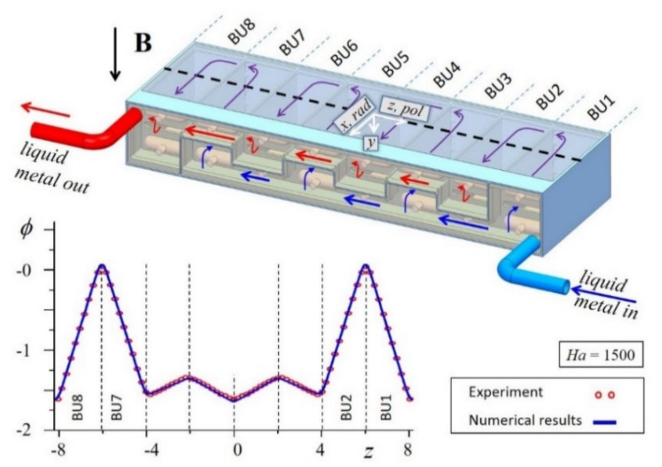
As mentioned above, a second class of experiments exists for the investigation of MHD flows in scaled mock-ups of entire TBMs. As an example, the results of potential measured on the surface of a mock-up for a HCLL TBM are shown in Figure 7. The test section consists of eight breeder units (BUs) which are fed and drained by a system of manifolds. From the experimental results (symbols) of the potential measurements in the middle of the module, it can be seen that higher gradients exist in external BU pairs, i.e., BU1-BU2 and BU7-BU8, while the values in the central ones are considerably smaller. Since potential gradients may be interpreted as an approximation of core velocities, it is obvious that there is a flow imbalance between external and central pairs of BUs. A numerical simulation of eight electrically coupled BUs agrees well with the experimental data on the middle plane of the mock-up and additionally yields details of the velocity profile, including flow in field-aligned boundary layers that cannot be detected from potential measurements on the Hartmann wall [73]. In this sense, numerical simulations and experiments are complementary.

The observation that external BUs receive more flow than the central ones is confirmed by measurements of pressure drop along typical flow paths in manifolds and BUs. This behavior originates from the design of manifolds whose cross-sections do not adjust to the changing flow rates when the fluid is distributed and collected along the poloidal direction.

More recently, the trend towards the development of PbLi MHD facilities gathers speed with the purpose of promoting integrated experiments and supporting TBM development. Related PbLi activities have been reported from China [74,75], India [76], Japan [77], Korea [78], Russia [79], Europe [80] and the USA, which operated the MaPLE facility [81]. The latter, initially built by the University of California Los Angeles, has been upgraded by a joint EU–US collaboration. It has been transferred to Europe and it is currently being reassembled at KIT, where it will contribute to the EUROfusion blanket program. MaPLE will provide experimental data on MHD heat transfer in blanket-typical geometries allowing different inclinations of the test section with respect to gravity and various orientations of the magnetic gap (horizontal, inclined, vertical). The ability to lift and tilt the 20-ton magnet to any desired position is a unique feature of this installation compared to other existing liquid metal facilities (see Figure 8). In MaPLE it is further planned to test measuring techniques to record pressure, flow rate and electric potential at reactor-relevant temperature and to gain experience in long-term operation of a PbLi MHD facility.

5. MHD Phenomena and Coupling with Heat and Mass Transfer

The occurrence of MHD effects can give rise to counterintuitive phenomena that can affect blanket performance. This is the case for flows in parallel electrically conducting ducts, in which electromagnetic forces induced by currents leaking across common walls modify flows in individual channels. Other examples are so-called coupled MHD phenomena, i.e., heat and mass transport in MHD flows. When multiple factors, such as induced currents and thermal gradients, determine the velocity distribution, the action of the resulting flow on material corrosion and tritium transfer is significantly different than in case of isothermal hydrodynamic conditions.

5.1. Electromagnetic Flow Coupling

When a LM moves in electrically coupled channels flow imbalance, reversal and recirculation may occur, which can cause the formation of regions of stagnant flow [25]. The latter is a primary concern for reactor safety, since it can lead to the accumulation of tritium and increased permeation towards coolant and structures, or to the formation of hotspots, in which the temperature exceeds the maximum allowable value of the structural materials.

5.1.1. Flow Distribution in Electromagnetically Coupled Parallel Channels

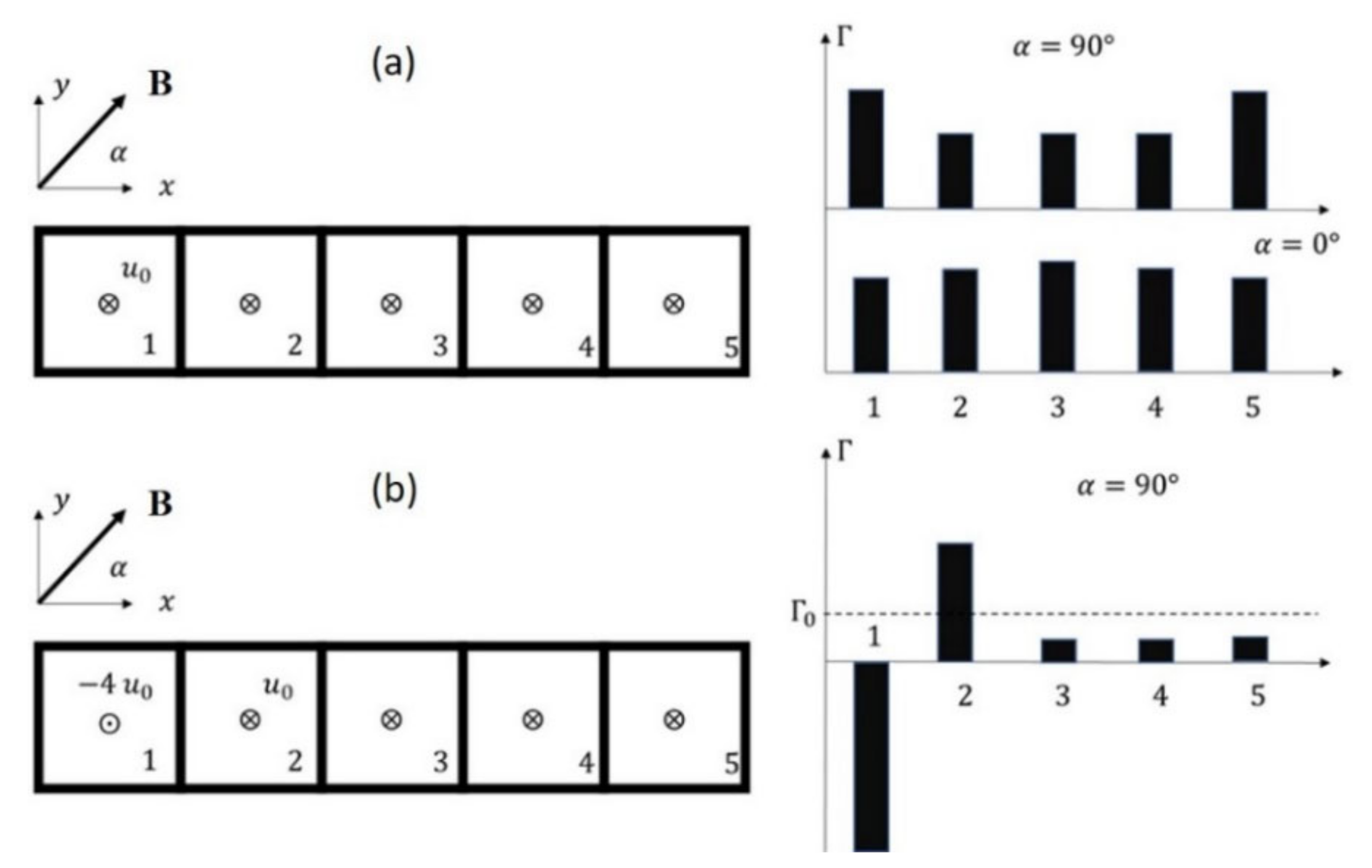
In Figure 9 an example of velocity distribution in five stacked electrically coupled ducts is depicted, where α is the angle between the horizontal coordinate x and the imposed magnetic field. In general, any inclination angle is possible between the two following limiting cases where:

• Channels are stacked along magnetic field direction, α = 0° (Hartmann wall coupling);
• Channels are stacked transverse to the magnetic field, α = 90° (sidewall coupling).

Let us consider the case of an array of channels where the flow in each duct is driven by the same imposed pressure head.

For α = 0°, mean velocity is predicted to increase in central channels [28]. Figure 9a shows qualitatively the variation of the flow rate depending on the duct number. Experiments conducted at the Efremov Institute [65] confirm the predicted effect and find a 13% increase in flow rate for the central duct in an array of three subchannels coupled at Hartmann walls.

For α = 90°, the velocity in each core is almost the same and sidewall jets in the boundary layers along the internal walls are suppressed. Because high-velocity layers, which are still present at external sidewalls, are able to carry a significant amount of flux, the flow rates in these external channels are increased compared to the inner ducts [82]. This effect is also qualitatively shown in Figure 9a.

Flow imbalance can also be observed when counter-flowing channels with different mean velocity are coupled through sidewalls (α = 90°). An example is found in the Lead Lithium Ceramic Breeder (LLCB) in which a number of ascending poloidal channels are electrically coupled with a descending return duct that carries their combined flow rates [83]. A qualitative representation of a similar case is displayed in Figure 9b. The high mean velocity in the return channel (no. 1) induces strong electric currents that leak in the adjacent duct and generate Lorentz forces. The latter ones draw more than double the flow rate into that channel from the manifold compared with the other ducts.

In general, in the breeding zone of a blanket, none of both limiting coupling modes exists. Solutions for 0° < α < 90° cannot be obtained just by superimposing the ideal cases described above. Only numerical simulations with a correct inclination of the magnetic field may reveal the complex physics determined by the electromagnetic flow coupling at common conducting walls, characterized by the spreading of internal layers along magnetic field lines [84]. When internal layers originating from singularities (e.g., corners) in one duct hit a common wall, the electromagnetic disturbance in potential and currents is transferred to the neighboring channel, in which the layer continues developing along field lines. This effect may even cause unexpected local flow reversal in parts of the neighboring channels depending on the driving pressure gradients. An example of flows coupled at common conducting walls and exposed to an inclined magnetic field (α = 67.5°) is displayed in Figure 10. Here, velocity contours are plotted on the cross-section of the channels together with the velocity profile along the central line of the duct array. Internal layers divide fluid regions inti cores with a uniform velocity that spans across the walls.

5.1.2. Coupled Flow in Manifolds of LM Blankets

Due to the complex geometry of fusion blankets and the fact that the major pressure drop arises from manifolds, it is not guaranteed that the driving pressure heads in all parallel channels of BUs are equal. The influence of manifolds on the flow in eight electrically coupled BUs of a HCLL blanket has been investigated experimentally and the electric potential measurements show that the BUs at the mock-up extremities are characterized by higher flow rates compared with central BUs (see Figure 7). The velocity profiles deduced from electric potential data are consistent with coupling through sidewalls and the strong difference in flow rates is linked to significantly different pressure heads driving the flow in individual BUs [73] (see also Section 4).

Electromagnetic coupling can also cause the appearance of flow reversals. This phenomenon is an issue in the breeding zone but particularly in the outflow manifold, where one wishes to avoid stagnation of the tritium-rich breeder. Coupling-mediated flow reversals may appear in co-flowing manifold channels of HCLL [85] or WCLL [30] blankets. They are associated with different flow rates or pressure heads between adjacent channels that, in turn, lead to an imbalance in mean flow velocity and leaking currents. For instance, the co-flowing feeding and draining manifolds in the WCLL TBM, in which flow rates reduce and increase, respectively, along the poloidal direction, are coupled through common conducting Hartmann walls [30]. At the top and bottom of the TBM, the mean velocity difference between manifold channels is the highest and currents leaking into the duct with the lower velocity tend to drive its core. The pressure build-up there leads to a reversed flow in the side layers that can reach a significant fraction of the flow rate.

As an example of a different manifold concept, we discuss the case of the co-axial manifold proposed for the WCLL blanket [31,86], where a reverse flow was observed even for equal imposed flow rate in the two concentric channels due to the higher mean velocity in the internal duct [31]. The flows in the two channels are along z, isothermal, steady and fully developed, and a uniform toroidal magnetic field is imposed in x-direction. The liquid metal enters the blanket through the external duct and exits it through the internal one. As a result, the external channel flow rate (Γ_in) decreases, moving towards the top of the blanket, while the internal duct flow rate (Γ_out) increases. Local flow reversals caused by electromagnetic coupling can be observed in Figure 11. In general, it is advisable to tailor the manifold configuration to ensure that all the channels have a similar mean velocity along their length in order to avoid coupling-mediated flow reversals.

5.2. Turbulence and Heat Transfer

Turbulent fluctuations in a flow of an electrically conducting fluid are suppressed by an imposed magnetic field via conversion of their kinetic energy into heat by Joule dissipation of induced electric currents. As a result, MHD flows are found in a laminar or transitional state at much higher Reynolds and Grashof numbers than their hydrodynamic counterparts. For example, transition to turbulence in isothermal flows in ducts and pipes with electrically insulating walls and an imposed transverse magnetic field occurs at Re growing with Ha so that Re/Ha remains in the range between 200 and 400 [87]. Even when turbulence occurs, it is transformed into an anisotropic state with suppressed flow gradients in the direction of the magnetic field lines [88,89,90].

Practically, the suppression of turbulent fluctuations by a magnetic field implies that conventional (three-dimensional, albeit anisotropic) turbulence can occur in typical blanket conditions only if poorly electrically conducting fluids, such as the molten salts FLiNaK or FLiBe, are used as working liquids. In that case, turbulent flows with high Re and moderate Hartmann number, Ha~100, are anticipated. The properties of such flows include decreased fluctuation amplitude, anisotropy, reduced rate of energy transfer to small length scales and the corresponding (steeper slope) transformation of the energy power spectrum. Moreover, reduced rates of turbulent transport, and development of flow regimes with localized turbulent zones and large-scale spatio-temporal intermittency are observed (see, e.g., [5,6,90,91,92,93,94]). Modeling of such flows can be accomplished by LES or RANS methods, but models have to be adapted for the peculiar nature of MHD turbulence (see, e.g., [5] and references therein for a discussion of this interesting topic). The models commonly applied in conventional hydrodynamics (for example, the $k-\epsilon$ model in RANS or the classical Smagorinsky model in LES) do not produce accurate results due to their excessive dissipation and inability to reproduce anisotropy and intermittency effects.

In the case of strongly electrically conducting fluids, such as PbLi, Ha~10⁴ typical for blanket conditions implies that 3D turbulence cannot occur. This does not mean that the flow necessarily becomes laminar and steady-state. From the general physical perspective, it is evident that even a very strong magnetic field cannot prevent the growth of hydrodynamically unstable perturbations, if the perturbations are quasi-two-dimensional (with nearly zero velocity gradients along the magnetic field outside the boundary layers) and, therefore, do not generate significant Joule dissipation. The physical nature of such instability may vary. For example, growth of perturbations has been demonstrated for shear-flow instability of the Kelvin–Helmholtz type, thermal convection, or a combination of the two (see, e.g., [95,96,97,98,99,100,101,102] or the review [5] for further examples).

The growth occurs in the absence of conventional turbulent mixing, in the conditions of quasi-two-dimensionality, and, typically, at high values of control parameters, such as Re or Gr. The often-observed outcome is an ultimate flow state in the form of unsteady regimes with strong inertia effects. The flows can be characterized as experiencing quasi-two-dimensional turbulence with friction imposed on the flow at walls perpendicular to the magnetic field. More important than this classification is that the properties of such flows are very different from the ones predicted at the same parameters by models based on assumptions of a steady-state and laminar or inertialess behavior. The flows are dominated by large-scale quasi-two-dimensional vortices and jets. Temperature oscillations of high amplitude (up to 50 K) and low frequency have been observed in experiments and obtained in calculations at moderately high Gr and Ha achievable in a laboratory [5]. The state of the flows at higher Gr and Ha typical for blanket conditions is debatable, but there are strong indications that fluctuations of even higher amplitude are to be expected [98,102]. Should such high-amplitude low-frequency fluctuations occur in components of a liquid metal blanket, potentially serious consequences include a substantial increase in the rates of transport of heat and tritium, the modification of balances controlling corrosion, and strong unsteady thermal stresses in the walls.

5.3. Tritium Transport

Tritium consumption for a 2000 MW fusion power reactor is about 112 kg per full power year, which is an enormous amount when compared with the actual worldwide availability, estimated as 20–30 kg [103]. Even if tritium can be produced from lithium, the bred tritium has to be almost completely recovered for subsequent use as fuel. This means that tritium self-sufficiency represents one of the most challenging issues for future deployment of fusion electricity. Therefore, an efficient characterization of processes and technical solutions to manage and control tritium transfer and release is mandatory.

For the development of liquid metal breeding blankets, the assessment of fusion reactor safety and the ability to breed tritium, it is necessary to accurately predict how tritium transport is affected by complex phenomena such as diffusion, surface reactions, MHD effects and heat transfer. Therefore, mathematical models and computational codes have to be developed to quantify tritium distribution, inventory, retention in PbLi and structural materials, and permeation losses from PbLi to the coolant, to the reactor building and the environment. Among the different phenomena affecting tritium inventories and losses, one should mention Sieverts’ law describing solubility in metals, but also surface reactions and the possibility of tritium becoming trapped in the structure.

Hydrogen isotope solubility in PbLi (Sieverts’ solubility constants), including that of tritium, suffers from uncertainties of up to three orders of magnitude depending on the adopted measurement technique (absorption or desorption). The huge difference between the two techniques needs to be better understood. For these reasons, experimental campaigns are being conducted in Europe in order to re-evaluate PbLi properties including crosschecking of data from different laboratories under controlled conditions of PbLi manufacturing and chemical composition.

For the determination of tritium inventory and flux in different materials, which are in contact, it is necessary to define suitable interface conditions. Tritium concentration $c_T$ (mol m⁻³) at a certain interface is linked to tritium partial pressure $p_T$ through Sieverts’ law [104]

$$c_T=k_S\sqrt{p_T},$$

(5)

where $k_S$ (mol m⁻³ Pa^−0.5) is the Sieverts’ constant. At the interface between liquid metal and steel, the continuity of $p_T$ is assumed,

$$p_{T,ls}=p_{T,sl},$$

(6)

where the subscripts ls and sl indicate the liquid phase at a steel interface and steel at an interface to a liquid, respectively. Substituting Equation (5) into Equation (6) yields a concentration discontinuity related to the ratio of Sieverts’ constants of liquid metal and steel, $k_{s,l}/k_{s,s}$, called the partition coefficient

$$\frac{c_{T,ls}}{c_{T,sl}}=\frac{k_{s,l}}{k_{s,s}}.$$

(7)

As a result, the uncertainty in the PbLi solubility directly translates into a lack of confidence in tritium permeation rate and inventories. To deal with these uncertainties in a conservative way, most of the tritium models use the lowest available solubility values, which provide the highest permeation rates from PbLi to the coolant.

Tritium permeation rate across interfaces of different materials is affected by surface conditions. Oxidized or clean walls have different properties, e.g., absorption, desorption, and recombination constants, with consequences on tritium permeation fluxes, especially at lower tritium partial pressures, i.e., when the limiting process characterizing the permeation is due to surface effects. The recombination constant, $\sigma k_2 \left[{\mathrm{m}}^4 {\mathrm{mol}}^{-1} {\mathrm{s}}^{-1}\right]$ is related to the Sieverts’ constant as $k_s^2=\sigma k_1/\sigma k_2$, where $\sigma k_1 \left[{\mathrm{mol} \mathrm{m}}^{-2}{\mathrm{s}}^{-1}{\mathrm{Pa}}^{-1}\right]$ is the dissociation constant and σ the sticking probability [105]. The recombination constant is strictly dependent on the condition of the material surface and therefore its value suffers from huge uncertainties. In addition, up to now consolidate reference values for transport properties in Eurofer are still lacking and properties of Optifer-IV steel are typically used instead.

In addition to the aforementioned uncertainty of physical parameters, tritium trapping in solid structures, which can result from impurities and material defects or neutron irradiation damages, can considerably affect tritium inventory and losses. The density of trap sites increases with the damage induced by neutron irradiation. Tritium implantation depends on the ion flux density and energy, and the peak implantation usually occurs at few nanometers under the surface of the metal. Permeation, therefore, depends on surface conditions of plasma-facing components and on defect traps, hence it can increase on contaminated surfaces.

Recent calculations with system-level codes for WCLL blankets estimate a total tritium release to the coolant without any mitigation strategy of 38 g/d, which is about 11.7% of the total tritium generated. This implies high tritium inventories retained in the water circuits, surpassing the safety limit in few days of operation [106]. Therefore, the reduction of tritium permeation is a primary issue for the licensing of a DEMO reactor [107].

In order to mitigate tritium release to the coolant two main strategies are foreseen. The first one concerns the adoption of efficient tritium extraction systems able to guarantee low inventories reducing the gradients of concentration, which are responsible for permeation phenomena. Among the different technologies, the most promising ones [12] are the Gas-Liquid Contactor (GLC), which is the reference technology for ITER, the Permeator Against Vacuum (PAV) and the Vacuum-Liquid Contactor (VLC). It must be kept in mind that the scalability of these tritium extraction units from ITER to DEMO has to be addressed from the point of view of technological feasibility and costs. A second approach to reduce tritium losses is the use of anti-permeation barriers (APB) [108]. This strategy appears to be required when considering practical and economic limits on the size and hence the efficiency of tritium extraction systems. The APB performance in terms of permeation flux reduction is quantitatively assessed by the Permeation Reduction Factor (PRF), which quantifies the ability to reduce the permeation of hydrogen isotopes. The PRF is defined as the ratio of tritium permeation fluxes through an uncoated wall ($j_{T_2}^{uncoated}$) to that across a coated one ($j_{T_2}^{coated}$),

$$PRF=j_{T_2}^{uncoated}/j_{T_2}^{coated}.$$

(8)

Several coatings have been proposed over the years [109], among which the most promising ones in terms of PRF are Er₂O₃, ZrN, Al-Cr-O, Al₂O₃. These coatings may guarantee PRF higher than 1000 in the range 400–700 °C. Alumina Al₂O₃ serves also to mitigate corrosion of Eurofer steel and represents the reference coating for DEMO [107]. Additional research is necessary in order to ensure high adhesive strength of coatings, compatibility with complex shapes, and good performance in a radiation environment.

5.3.1. Tritium Analysis Methods, Transport Modeling and Coupling with MHD

Tritium transport in blankets is complex, since it includes many different phenomena and involves a large number of physical properties and parameters, many of which have not yet been determined with an adequate level of accuracy. Moreover, simplified models, which use empirical coefficients and are employed to obtain a first estimate of tritium inventory, have often limited applicability in terms of operating conditions. Therefore, they are less relevant for DEMO applications. The physics included in modelling tools for investigation of tritium cycle in fusion blankets should have a sufficient complexity, in order to support the design of TBMs and the definition of the experimental program for ITER. Additionally, models should allow exploiting experimental data from ITER and to extrapolate them to DEMO conditions. A four-step structure of the development strategy for tritium transport modeling tool is presented in [110]. It is proposed to keep a modular structure of the predictive tool, starting from the description of single components and by including progressively subsystems, such as TBM and ancillary systems, up to the complete test blanket system.

Tritium analyses can be performed either by employing system-level models for computing the global performance of blankets and ancillary systems, or by detailed 3D models and numerical simulations for spatially limited domains and critical regions. System-level models, which are discussed in more detail in Section 3.3, consider at most 1D equations [111]. Flowing PbLi is taken into account via imposing a mass transfer coefficient at interfaces between liquid metal and walls. This is the case of TMAP7 [112], FUS-TPC [113], EcosimPro or mHIT [114], which have been used for estimating tritium transport and inventory in different blanket concepts and divertors, and performing parametric sweeps. Exercises of verification of these codes against analytical solutions, validation against experimental data and benchmarking between them have been performed [112,114]. Most of the validation procedures are performed in solid systems and are devoted to validating processes such as diffusion, surface recombination, chemistry reactions, trapping, etc. System-level codes present important limitations when dealing with MHD coupling, since correlations between the Sherwood, Reynolds and Hartmann numbers are not known in blanket conditions. The Sherwood number Sh describes the ratio of effective mass transfer to the rate of diffusive mass transport. Therefore, these codes use either classical hydrodynamic correlations or an analogy with heat transfer. However, the latter type of correlations has been derived for relatively low Hartmann numbers ($Ha<375$ [39]) and they are not applicable to blanket conditions.

Regarding detailed models, various finite volume and finite elements models have been developed for simulating tritium transport coupled with MHD effects. Several academic codes typically use the outputs of available MHD solvers as input for the velocity field in the calculations of mass transfer. This includes, for example, the case of CATRYS [115], which solves the equations for tritium transport and uses the velocity field from the MHD HIMAG code as input. Other tritium transport codes have been developed with an integrated MHD solver (e.g., [116]).

Another category comprises 3D simulations with commercial multiphysics codes, such as ANSYS-Fluent and COMSOL-Multiphysics. These simulation platforms include customization capabilities, where MHD modules can be integrated into available fluid dynamic solvers. For validation of non-MHD mass transfer in these codes, there are few facilities available where hydrogen isotopes are dissolved in flowing PbLi, as described in [117] or the recently constructed CLIPPER loop [118] at CIEMAT. At ENEA Brasimone, the TRIEX-II facility is able to qualify GLC, PAV and VLC technologies at different temperatures, PbLi mass flow rates and hydrogen isotopes concentrations [119]. Unfortunately, in none of the existing facilities can a magnetic field be applied on a section of the flow path.

Because of this experimental limitation, tritium transport codes have been validated using experiments under hydrodynamic conditions or verified against analytical solutions [120,121,122]. These exercises do not ensure code validation in MHD flows, but once the hydrodynamic transport of dissolved species has been verified, there is high confidence that the transport equations for passive scalars are implemented in a correct way, taking into account all relevant physical phenomena and applying them to MHD velocity distributions as well. The degree of uncertainty in numerical modeling, due to a lack of validation against MHD experiments, seems far less compared to the poor knowledge of physical parameters (orders of magnitude differences) required for the simulations.

5.3.2. Tritium Transport under Fusion-Relevant Conditions

WCLL DEMO blanket. A number of studies have been performed to address the effect of MHD on tritium transport for the WCLL blanket concept for DEMO reactor [123,124]. In particular, flow in a portion of the breeding unit, as shown in Figure 12 on the top, has been simulated adopting a novel coupling strategy for the physics involved, and differences between pure hydrodynamic (Gr = 4.78 × 10¹⁰, Ha = 0) and magnetohydrodynamic (Gr = 4.78 × 10¹⁰, B = 4 T, Ha ≈ 11,000) conditions have been highlighted. In both models, the system has been assumed to be operated at steady-state conditions. Buoyancy effects have been introduced using the Boussinesq approximation. The radial profile of the volumetric nuclear heating on the equatorial midplane has been determined by means of the MCNP Monte Carlo code.

Figure 12 shows the comparison between the velocity field on a radial–poloidal plane in the middle of the central submodule of the BU for the two cases. The presence of the magnetic field changes completely the velocity distribution and its magnitude. Near the piping region, the PbLi is quasi-stagnant in the hydrodynamic case in Figure 12a, whereas in the MHD case (Figure 12b), jets are found near the electrically conducting walls parallel to the toroidal magnetic field and a fast recirculating zone, driven by buoyancy forces, occurs between the pipes.

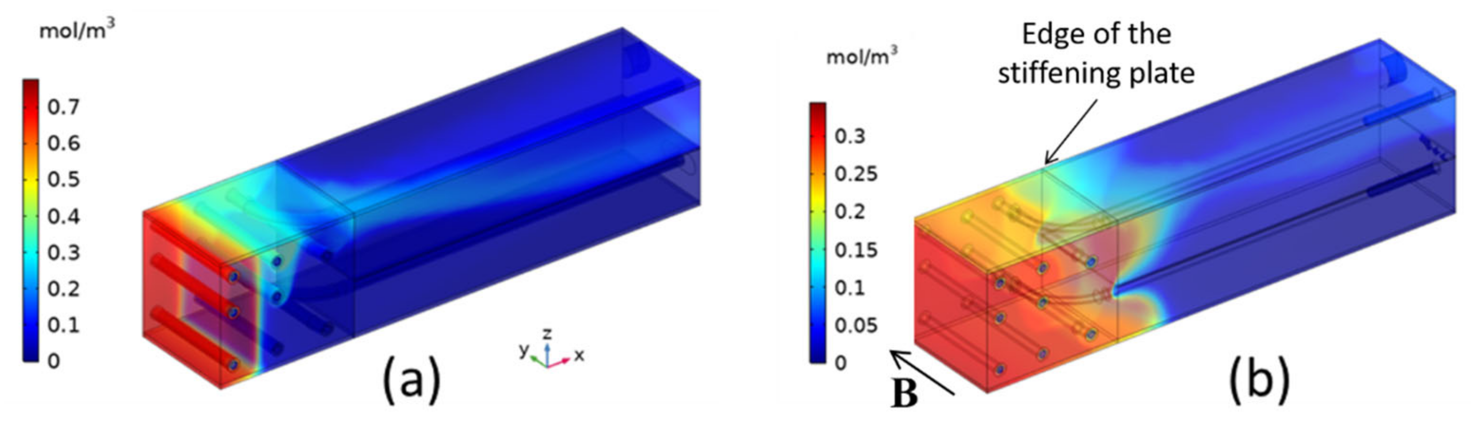
The MHD velocity distribution has, as expected, a significant effect on tritium transport. In the performed analysis, the Sieverts’ constant of tritium in PbLi is the one proposed by Reiter [126]. In Figure 13, the steady-state tritium concentrations in the PbLi and Eurofer domains are shown for the hydrodynamic and MHD cases. In the former one, most of the tritium is found in the zone between the first wall and the first pipe column, reaching values greater than $0.7$ mol/m³. By applying a toroidal magnetic field, the concentration is much more evenly distributed between the first wall and the edge of the stiffening plate, and the maximum value is smaller than $0.4$ mol/m³. Nevertheless, the presence of recirculation zones increments the tritium mean permanence time in the breeder unit, and the tritium concentration decreases rapidly with the radial coordinate.

The major effect caused by the different velocity fields is on the distribution of the tritium fluxes out of the blanket. In Figure 14, the comparison between the tritium that leaves the BU in the PbLi (Out) and the tritium that permeates through the piping system into the water (Permeation) is shown. As evident, MHD has a beneficial effect, and the permeation rate is reduced by around 60%.

Concerning tritium inventories in PbLi, Eurofer and water, there is no significant difference between hydrodynamic and MHD cases. Only a slight reduction in water has been found in case of MHD flow.

DCLL breeding blanket. The DCLL blanket concept is characterized by relatively high PbLi velocities compared to the WCLL blanket. The MHD pressure drop is reduced by electrically decoupling the PbLi flow from the metallic structure by using insulating Flow Channel Inserts (FCI) [127]. In the case of the European DCLL blanket design [128], a sandwich-type insert is proposed, which consists of a thin alumina layer protected by two Eurofer sheets. The FCI divides the flow into two regions: the core flow and the gap flow between insert and wall.

From the tritium transport perspective, the latter is probably the most critical region in the DCLL blanket. This is due to the fact that, since alumina is a very effective permeation barrier, only the tritium generated in the gap is suitable to permeate into the coolant. Assuming that the alumina is a perfect electrical insulator, fully developed models of the gap flow can be applied independently from the flow in the core. This kind of simulation has been launched using the ANSYS-Fluent MHD solver.

In Figure 15 (left) the velocity profile in the gap is shown for the pressure-driven MHD flow at $Ha=7630$ and $\partial p/\partial x=1740$ Pa/m representative for the frontal channel of the central outboard module. The resulting flow is characterized by quasi-stagnant PbLi regions in the gaps perpendicular to the magnetic field (Hartmann gaps), while most of the flow goes through the gaps parallel to the magnetic field (side gaps). The obtained velocity profile has been used as input for a 3D tritium transport model of the complete annular channel between external wall and FCI. This model considers an exponentially decreasing volumetric tritium generation along the radial direction and constant transport properties [129].

Figure 15 (right) displays concentration contours in the midsection of the channel. In spite of the volumetric generation being maximal next to the FW, the high-velocity jets in the side gaps are able to effectively transport most of the tritium to the channel outlet. In steady-state, this results in low tritium concentrations in the parallel gaps and larger concentrations in the quasi-stagnant Hartmann gaps. Inside these gaps, the concentration decreases with the radial direction. This is a consequence of the exponential shape of the tritium source. Analogous conclusions are described in [115], showing the causal connection between very low velocities in the Hartmann gaps and larger tritium concentration.

In Figure 15 (right) the concentration discontinuity due to the different solubilities of PbLi and Eurofer can be observed at both PbLi/wall and PbLi/FCI interfaces. There is one order of magnitude of difference in tritium concentration in side and Hartmann gaps. The steady-state permeation rate, from the gap flow into the helium channels, is around six times higher than the value predicted by a system-level model that considers an evenly distributed flow rate through the gaps [129]. This comparison highlights the need for 3D transport models to predict tritium distribution in liquid metal blankets in order to reduce uncertainties and inaccuracy caused by assumptions, geometrical approximations and simplifications of the physics, as used in system models. In particular, the MHD velocity distribution and the complexity of the blanket configuration have a noticeable influence on the results.

In [130] parametric studies have been carried out to quantify the major factors that govern tritium transport and permeation in the DCLL blanket. Tritium solubility significantly affects these phenomena, since it directly influences tritium partial pressure. The parameters that determine the velocity distribution in the liquid metal gap between FCI and wall, such as Hartmann number, FCI and wall electrical conductivity, also have a strong impact on the tritium permeation rate.

5.4. Corrosion

In the frame of blanket engineering for DEMO and ITER, the chemical compatibility of Reduced Activation Ferritic-Martensitic (RAFM) steel Eurofer in contact with the corrosive flowing liquid PbLi represents a serious problem for fusion blanket development. Along with the possible wall thinning in the hotter part of the liquid metal loop that could lead to a deterioration of the mechanical integrity of the blanket structure, critical safety issues are related to the transport of corrosion products in the PbLi loop [131]. They can be activated by the intense neutron flux giving rise to local accumulation of activated materials in the liquid metal system. Moreover, their precipitation in its cold section results in the potential plugging of the loop.

Corrosion in heavy liquid metals originates from physical-chemical phenomena involving the dissolution of the alloying elements, their transport, chemical reactions with dissolved non-metallic impurities (oxygen, nitrogen, etc.), and the formation of intermetallic compounds with the liquid metal and/or other dissolved metal impurities [132].

In PbLi environment, RAFM steels experience degradation phenomena mainly related to solution-based mechanisms [133,134,135]. In particular, almost-uniform dissolution of the main alloying elements (Fe, Cr) is observed on the exposed surface, and subsequent penetration of PbLi along grain boundaries. The higher diffusion rate of Cr in PbLi and its slower diffusivity in the steel matrix result in a selective leaching up to some µm of depth at the interface, with consequent surface enrichment of the low-solubility elements (e.g., W in Eurofer) [134,135]. Porous Cr-poor ferrite with PbLi penetration is then formed at the surface. Interactions with dissolved impurities such as O and N have not been reported.

Corrosion experiments carried out over the last two decades on RAFM steels have shown that corrosion occurs in two steps [136]. The first one consists of the non-uniform dissolution of the native oxide layer on the steel surface. This process occurs during the “incubation time”, whose duration depends on PbLi temperature and flow. The second step is the dissolution of the bulk via leaching of Fe and Cr. According to some experiments, the incubation time for RAFM steels in flowing PbLi is shorter than under stagnant conditions and is reported to be 500 h at 550 °C [137] and it can last up to 1000 h at 480 °C [138].

Besides the effect on the incubation time, PbLi temperature and fluid-dynamic conditions are the main parameters that influence the rate of corrosion of RAFM materials [133,137,138]. Larger temperature enhances the dissolution effect because of the increased solubility and diffusivity of the alloying elements in the liquid metal. The increased flow rate and the transition from laminar to turbulent regime raise the mass transfer in boundary layers. Finally, erosive effects, such as the spall-off of the porous Cr-poor ferrite layer, are inherent to flowing conditions. This is shown by experimental studies that found a corrosion rate for Eurofer steel at 550 °C of about 400 µm/yr at 22 cm/s [137], 220 µm at 10 cm/s [133], and 18 µm in static PbLi [135]. The strong impact of elevated temperature becomes obvious when corrosion rates are compared with results for lower temperatures for which, e.g., at 480 °C, rates of only 90 µm/yr at 22 cm/s are observed [138].

Dissolved corrosion products and impurities are reported to have an influence on the corrosion of the materials in PbLi in isothermal systems, since they reduce the corrosion rate of steel in comparison with “fresh” melt [139]. However, dissolved corrosion products are expected to participate in re-crystallization and deposition phenomena in colder sections of non-isothermal dynamic systems, such as PbLi loops. Crystallized particles may move with the melt flow or be deposited on colder surfaces where plugging may occur in the narrow sections, affecting PbLi circulation.

5.4.1. Modelling of Steel Corrosion in PbLi

Although the PbLi loop piping will be internally coated by alumina ceramics to face the high corrosiveness of PbLi and to reduce tritium permeation to the coolant and environment [109], theoretical predictions are needed to assess the feasibility and safe operation of breeding blankets for DEMO and ITER. Modelling tools have to be validated against experimental data [140]. Several experimental campaigns have been performed to study the corrosion of RAFM steels in flowing PbLi. Some of the most relevant recent results are reported in Table 3 and briefly described in the following.

The PICOLO loop at KIT (Germany) was extensively used to perform long-term exposure of different RAFM steels (Manet I, F82H-mod, Optifer IVa, CLAM), Eurofer and ODS-Eurofer at 480 and 550 °C in turbulent flowing conditions (10 and 22 cm/s) up to 12,000 h [133,137,141,142]. The loop has a “figure-of-eight” configuration, with a cold leg equipped with magnetic trap, electromagnetic pump, and magnetic flow meter.

LIFUS-2 loop at ENEA (Italy) was used to test Eurofer steel at 480 °C in laminar flowing conditions (1 cm/s) up to 4500 h [143]. In the “figure-of-eight” loop PbLi flow rate was ensured by a mechanical pump in the cold leg. An upgraded configuration was recently proposed to study the effect of the dissolved impurities, including cold-trap, sampling system for PbLi chemical analysis and the use of a coating on the internal piping of the loop [144].

DRAGON PbLi loop series at INEST-CAS (China) are foreseen to study PbLi corrosion in both thermal and forced convection conditions [75]. The DRAGON-IV loop was also constructed to investigate the corrosion behavior at high temperature (480–800 °C) with flow up to 1 m/s under magnetic field (B = 2 T) and stress-applied conditions in PbLi.

An Indian loop was also recently put in operation at IPR (India) to study PbLi corrosion. An experimental campaign on IN-RAFM steel was conducted in flowing PbLi at 465 °C, 10 cm/s up to 5000 h [136].

Table 3. Most relevant corrosion data of RAFM steels in flowing PbLi.

Material	Loop	Thot °C	Tcold °C	Velocity m/s	Corrosion µm/year	Reference
IN-RAFM	Indian	465	400	0.10	31–44	[136]
Eurofer	LIFUS 2	480	400	0.01	40	[143]
Manet I, F82H-mod, Optifer IVa, Eurofer	PICOLO	480	350–400	0.22	90	[138]
CLAM, Eurofer, ODS-Eurofer	PICOLO	550	400	0.10	200–220	[141,142]
Eurofer	PICOLO	550	400	0.22	400	[137]

Table 3. Most relevant corrosion data of RAFM steels in flowing PbLi.

Material	Loop	Thot °C	Tcold °C	Velocity m/s	Corrosion µm/year	Reference
IN-RAFM	Indian	465	400	0.10	31–44	[136]
Eurofer	LIFUS 2	480	400	0.01	40	[143]
Manet I, F82H-mod, Optifer IVa, Eurofer	PICOLO	480	350–400	0.22	90	[138]
CLAM, Eurofer, ODS-Eurofer	PICOLO	550	400	0.10	200–220	[141,142]
Eurofer	PICOLO	550	400	0.22	400	[137]

During experimental campaigns, correlations have been identified in order to explain the experimental results from loop facilities and to extrapolate data to other operating conditions. For instance, Sannier’s correlation serves to calculate the metal loss of steels at a given temperature and PbLi flow rate in turbulent/mixed regime [145]. Good agreement between experimental results was found for data obtained from PICOLO and the Indian loop on Eurofer and RAFM steels [133,136], but no consistency was found for data in the laminar regime, which exhibit some scattering.

Since corrosion in fusion blankets is a complex phenomenon that includes kinetics of solution and deposition mass transfer and interaction with impurities, the development and validation of modelling tools is necessary for predictive design input data. To date, the code MATLIM found validation against corrosion data of RAFM steels in turbulent/mixed regime [140,146], but validation still needs to be performed in laminar conditions, as expected in BUs of WCLL blankets, where the PbLi velocity is few mm/s. Hence, experimental campaign in relevant conditions of flow and thermal gradients should be performed for code validation, also considering the effect of magnetic field and applied stress.

For reliable application of predictive tools, values for solubility and diffusivity of dissolved species have to be known with better accuracy. These properties are very important for the implementation of models as they reflect the mass transfer coefficients [140,145]. Solubility values of Fe in PbLi were obtained experimentally by various authors, but they differ by orders of magnitude [147]. The solubility value of Cr is completely missing. In addition, in most of the experimental campaigns no monitoring of impurity levels, e.g., of dissolved metals and non-metal impurities, has been performed [140]. The presence of dissolved corrosion products and the formation of precipitates affect the evaluation of corrosion rates during the tests. Moreover, the influence of impurities, such as H, O, N, on the corrosion of structural materials has never been investigated experimentally.

5.4.2. Corrosion with Magnetic Field

A review of possible effects of a magnetic field on corrosion and deposition in flowing PbLi is given in [148]. The major influence of the magnetic field on corrosion processes is related to the change in the velocity profile due to the action of the induced electromagnetic forces, which results in steeper velocity gradients in the near-wall region and modified transport properties in the flow. Depending on the electric characteristics of the wall material, the flow rate inside the boundary layers at the walls parallel to the magnetic field can reach very large values. The thickness of the boundary layers reduces with increasing magnetic field strength; hence, the diffusion layer becomes thinner. Moreover, MHD flow in electrically coupled ducts can be characterized by flow reversals (cf. Section 5.1), and turbulent MHD flow is typically anisotropic with formation of Q2D turbulent structures (see Section 5.2). All these aspects determine the velocity distribution close to the fluid–solid interface, which controls mass transfer phenomena. In addition to that, the effect of the magnetic field on chemical reactions at the material surface should be taken into account, together with an electrodissolution mechanism due to induced currents entering the walls, as discussed in [149] for the corrosion of Hartmann walls.

Only a few experimental investigations are available in the literature in which the influence of a magnetic field on steel corrosion is studied, as required for fusion applications.

The compatibility of PbLi with austenitic (316 L) and martensitic (1.4914) steel under the influence of an imposed magnetic field (1.4 T) perpendicular to the module axis has been analyzed in the devices CELIMENE and ALCESTE [150,151]. The liquid metal (PbLi) was filled in a 30 mm annular space between a hot and a cold tube. In the former loop, the weak flow was due only to natural convection; in the second one, equipped with an electromagnetic pump for PbLi circulation, the mean velocity in a section was about 1 mm/s. It was observed that by applying a magnetic field, the corrosion rates of the two types of steel in semi-stagnant LM increase by about 50% for 316 L steel and 30% for 1.4914 steel compared to hydrodynamic conditions. The corrosion process is mainly due to dissolution of iron in the liquid metal. Concerning the deposition rate, it was found to be larger in the direction parallel to the magnetic field.

At IPUL (Latvia) experiments with samples of both P-91 steel [152,153] and Eurofer [154] have been carried out to study the influence of a magnetic field on corrosion phenomena in flowing PbLi. The loop consists of a cold and a hot part. The test section with samples is located partly in the magnetic field and partly outside, so that corrosion rates in hydrodynamic and MHD flows can be compared.

In this loop, non-isothermal corrosion of Eurofer steel has been investigated in a PbLi flow with a mean velocity of (5 ± 0.5) cm/s, a maximum operating temperature of 550 °C and a magnetic field of 1.7 T [154]. During a 2000 h experimental session, an intensification of corrosion processes was observed due to the presence of the magnetic field. Mass losses for the samples in the magnetic field were 1.5 ÷ 2 times higher than for the ones in the region with B = 0. It was also observed that samples in hydrodynamic conditions had a rather smooth surface, while those in MHD flow had a regular wavy pattern on the Hartmann walls, in the form of grooves oriented in the PbLi flow direction [155,156]. A more detailed observation of the sample surfaces revealed that, differently than in hydrodynamic flow, where corrosion takes place predominantly at grain boundaries, when applying a magnetic field, the bulk is also involved in the process due to a deeper dissolution. The diffusion of elements (e.g., Fe and Cr) from Eurofer into the liquid metal is enhanced by the magnetic field (faster erosion) [156]. Experimental results have also shown that the Eurofer corrosion rate is significantly affected by the temperature of the melt.

Experimental corrosion data of FM steels in flowing PbLi, in the presence of a magnetic field, are summarized in

Table 4. Experimental corrosion data of FM steels in flowing PbLi with magnetic field.

Material	Loop	Thot °C	Tcold °C	Velocity m/s	B T	Exposure h	Corrosion µm/year	Ref.
P-91 steel	IPUL/Riga	550	370–430	0.15–0.3	1.7	1000–2700	320–360	[152,153]
				0.15–0.3	Entrance	1000–2700	200–226	[152,153]
				0.15–0.3	Exit	1000–2700	100–218	[152,153]
Eurofer				0.05	1.7	1000		[156]
				0.05	1.7	2000	+50 ÷ 100%	[154]
		550	350	0.05	1.8	1000	+80 ÷140%	[155]
		515	350	0.05	1.8	2500	+80 ÷ 180%	[155]
316 L 1.4914	CELIMENE ALCESTE	thermal gradient DT = 40K, convection		0.001 and 0	1.4		÷50% +30%	[151]
316 L	CELIMENE annular geometry	thermal gradient		Natural convection movements	1.4	Corrosion rate in quasi- stagnant conditions is larger on average than with B = 0 Magnetic field results in dissymmetry between dissolution and deposition rates in directions ⊥ or θ to B		[150]

. When available, the results for hydrodynamic conditions with the same parameters are also indicated for a direct comparison.

A small number of theoretical investigations have been carried out to predict corrosion of Eurofer in PbLi exposed to a magnetic field. Data related to the diffusion coefficients of metallic elements in liquid PbLi are very limited; for instance, values of diffusivity and saturation concentrations of iron in PbLi exhibit a large scattering. The latter parameter is one of the most important in corrosion models, such as the one developed by Smolentsev et al. [147]. The code called TRANSMAG uses a fully developed 2D MHD flow model and solves in 3D mass and heat transfer equations. In [147], in order to improve the available data on the saturation concentration of iron, the values for this property are reconstructed from experimental results in turbulent hydrodynamic flow by solving an inverse problem. The obtained data are approximated by a new correlation, which is employed to predict corrosion in laminar MHD flow in rectangular channels. The results confirm the experimental observations: the corrosion rate increases when imposing a magnetic field, the appearance of the corroded surface depends on the orientation of the wall with respect to B, and a larger mass loss occurs at the sidewalls (2–3 times stronger corrosion rates if compared to the Hartmann wall). These studies highlight the need for further experimental campaigns to increase the amount and the accuracy of corrosion data in MHD flows. Moreover, the method used to achieve improved correlations for the properties needed for corrosion modelling by matching calculated and experimental data, represents a valid procedure to obtain reliable predictions of corrosion rates in MHD flows.

Numerical investigations of corrosion have been also carried out in MHD turbulent flows [157,158]. Since the magnetic field tends to suppress turbulent motions, smaller corrosion rates were found compared to the case B = 0, in contrast with observations in MHD laminar regime. The reduction of the corrosion rate depends on the orientation of the magnetic field with respect to the flow direction, due to the anisotropic action of Joule dissipation, and on the intensity of the field. A magnetic field perpendicular to duct walls leads to the largest reduction in the corrosion rate [157].

6. Conclusions and Future R&D

The development of engineering designs for liquid metal TBMs for ITER and blankets for a DEMO reactor requires profound knowledge about magnetohydrodynamics coupled with multiphysics phenomena such as heat transfer, neutron physics, tritium breeding and transport, and the corrosion of wall material.

The progress in the numerical modelling of MHD flows combined with the availability of high-performance computing makes it possible to attain detailed insights into flow properties (pressure, velocity, temperature, electric potential) for various types of geometries and parameters close to those in fusion applications. There exists good confidence in the validity and accuracy of predictions, since numerical codes have been carefully validated against analytical solutions and model experiments. Often experiments and theoretical analyses are complementary since measured data are required for code validation or derivation of design correlations, and numerical results may support the interpretation of experimental observations.

The complexity of engineering designs represents a challenge for the numerical prediction of MHD flows in blanket-relevant geometries, since it implies special requirements for grid generation and for the employed numerical schemes. The computational meshes have to provide reasonable resolution of boundary layers, but, unlike in hydrodynamics, they also have to account for thin internal layers that spread along field lines from wall singularities and electrical discontinuities. Future research should find strategies for automatic grid generation that consider these particular needs. Discretization algorithms have to preserve conservation of mass, momentum, internal and kinetic energy, and electric charge.

Numerical investigation of coupled MHD effects in liquid metal blankets by means of CFD codes has achieved remarkable progress in recent years in terms of prediction accuracy and the complexity of the geometry and physics that can be modelled. However, even by using HPCs, simulations of large problems are still very time-consuming. Therefore, the use of SYS-TH codes for fusion applications represents a valuable option that should be significantly promoted. As pointed out, the prediction of MHD effects in liquid metal blanket systems by means of SYS-TH codes is still very challenging and far from suitably mature. Pressure drops in blanket components and heat transfer can be well described by friction coefficients and Nusselt number correlations. On the other hand, further effort should be put into the determination of reliable closure laws for the description of coupled MHD phenomena, such as electromagnetic coupling and mass transport, and for the prediction of blanket accidental transients. A number of studies are available in the literature on coupled system/CFD codes for thermal-hydraulics and safety analyses for nuclear reactors. Methods of coupling, of data transfer processing between CFD and system codes, as well as validation procedures have been reviewed in [159] and they may also be applied in fusion engineering.

Apart from heat transfer, where buoyancy may directly affect the flow, all other coupled phenomena may be considered as convective diffusive transport problems of passive scalars, i.e., dissolved tritium or corrosion products. The inventory and flux of dissolved species can be described by a convection–diffusion equation and the solution is straightforward as in hydrodynamics, once the PbLi velocity is known from MHD analysis. The major drawback in these analyses is the low precision of thermophysical properties such as solubility and diffusivity, since their reported values in the literature differ by orders of magnitude, as well as unknown kinetics of reactions at interfaces. As a result, the major uncertainties in theoretical predictions derive from scattering in the temperature-dependent thermophysical properties of PbLi required for the analyses. Smolentsev et al. [147] showed the importance of exploiting the synergy between experiments and simulations in order to obtain more reliable correlations for parameters used, for instance, in the numerical studies of corrosion in MHD flows. As long as precise input data for numerical simulations are not available, sensitivity studies by varying the uncertain quantities in a wide range may be used to achieve preliminary conservative estimates for corrosion rates or tritium permeation losses.

Once a precise measurement of material properties is available, target-oriented benchmark experiments have to be performed to validate models for tritium and corrosion transport in MHD flows. For instance, models for tritium transfer analysis are validated only against hydrodynamic experiments, and validation of the implemented coupled phenomena is missing. Therefore, experimental data are essential to increase the reliability of these models.
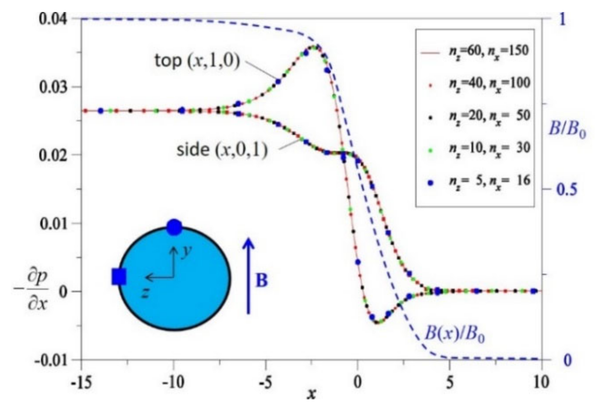
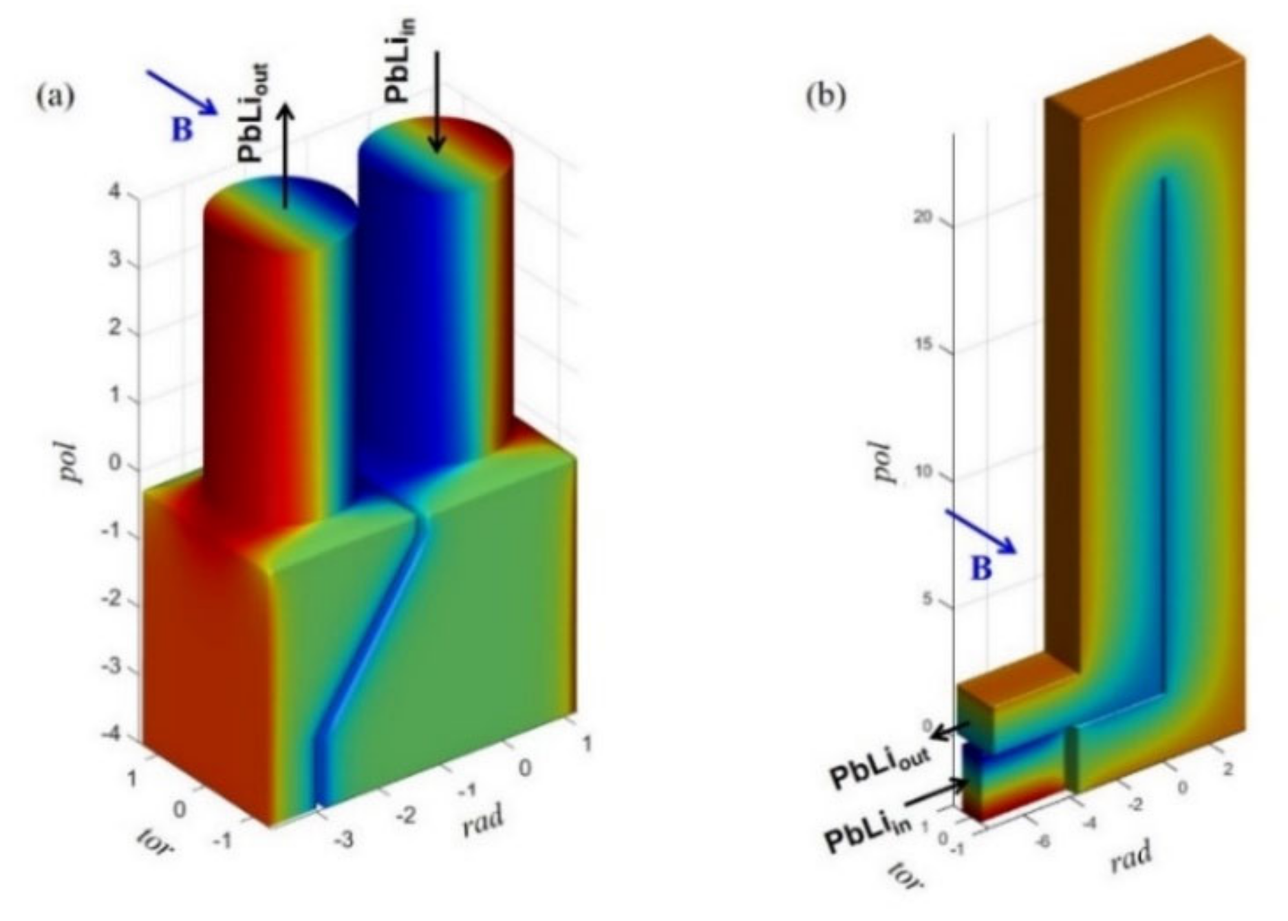
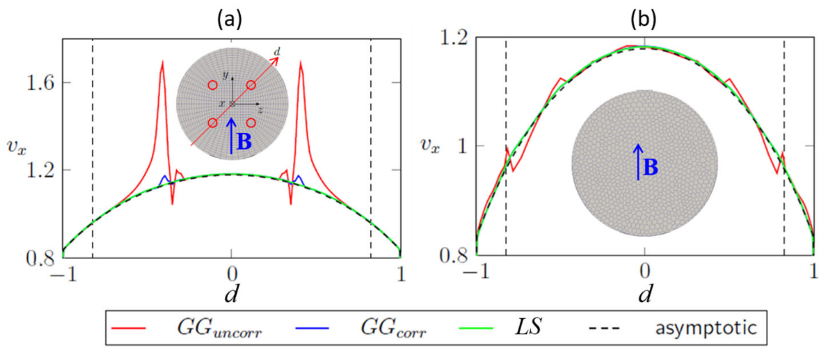
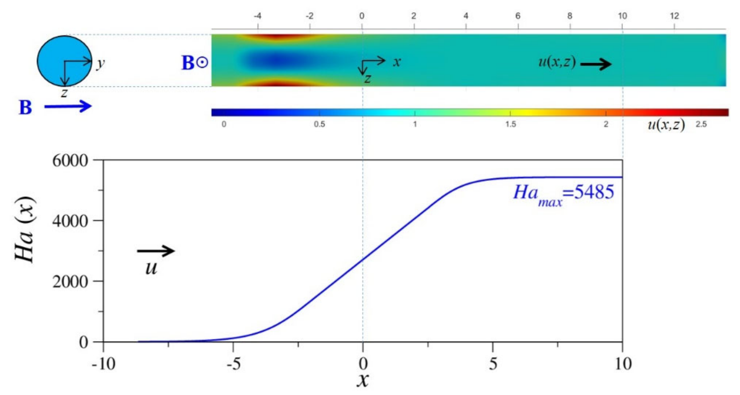
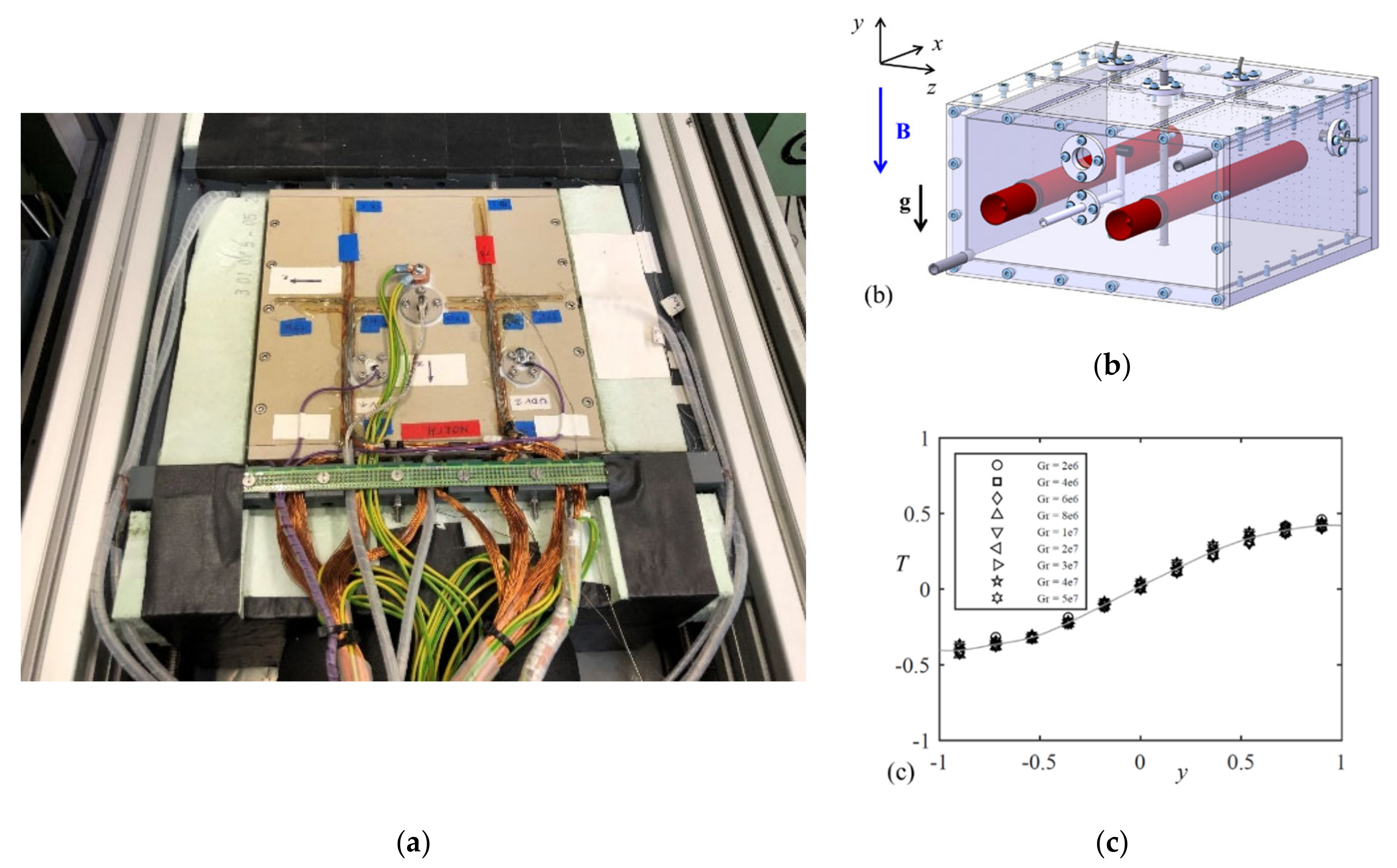
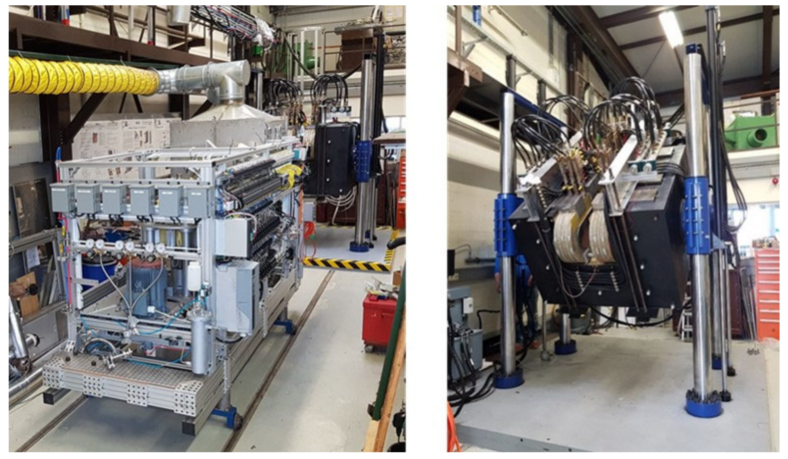
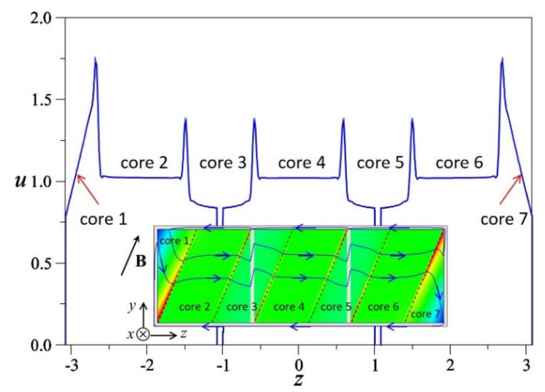
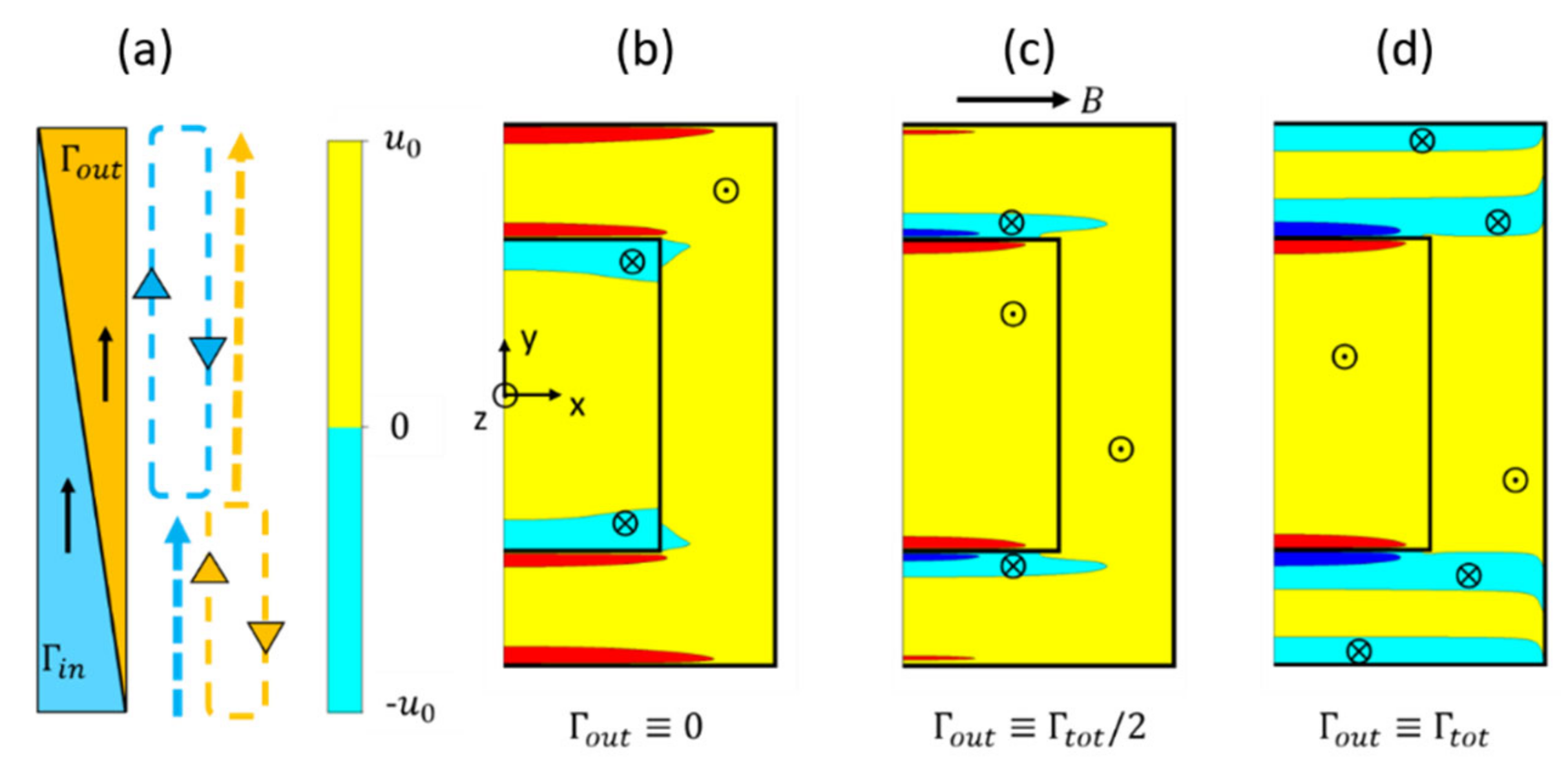
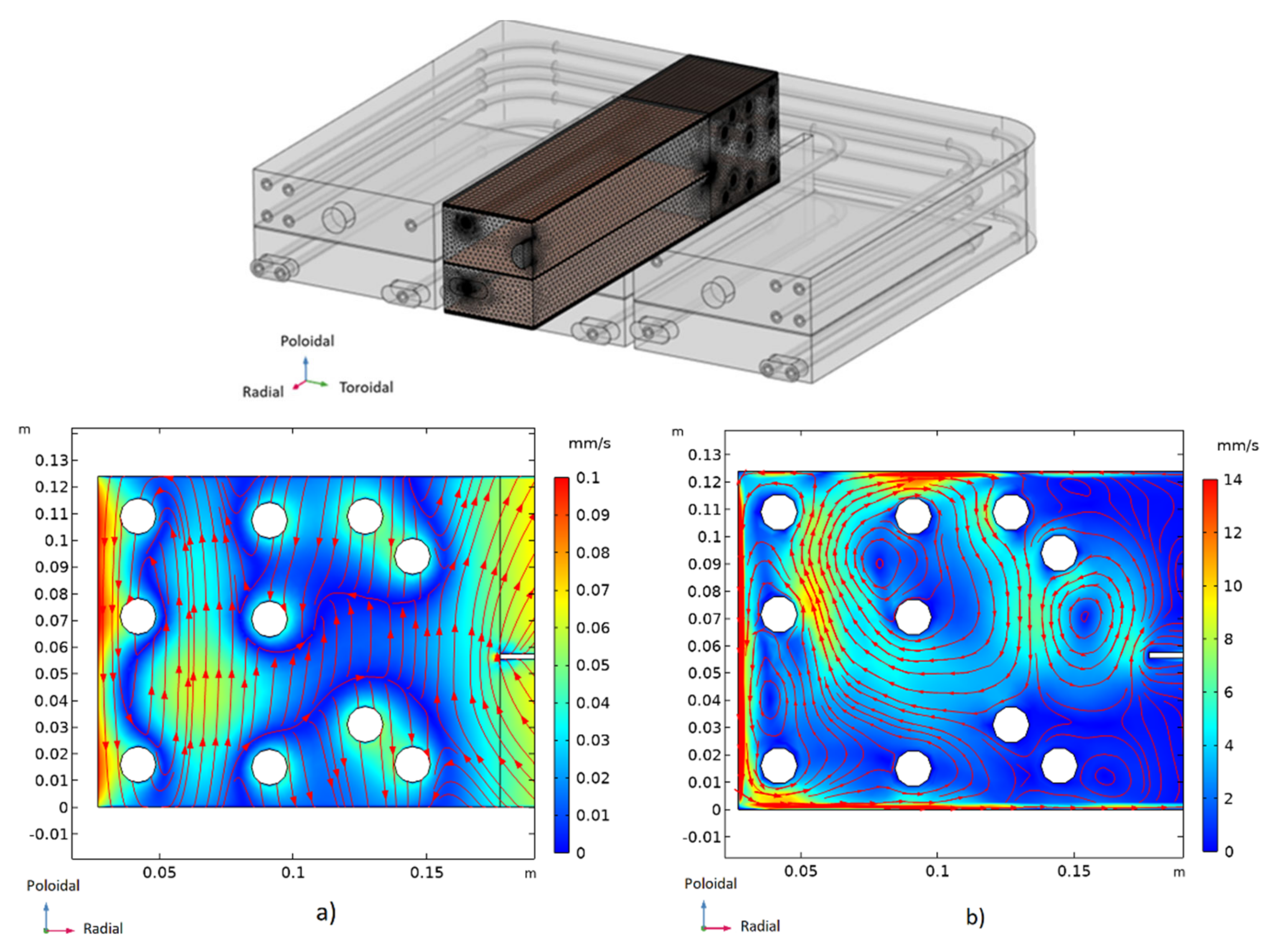
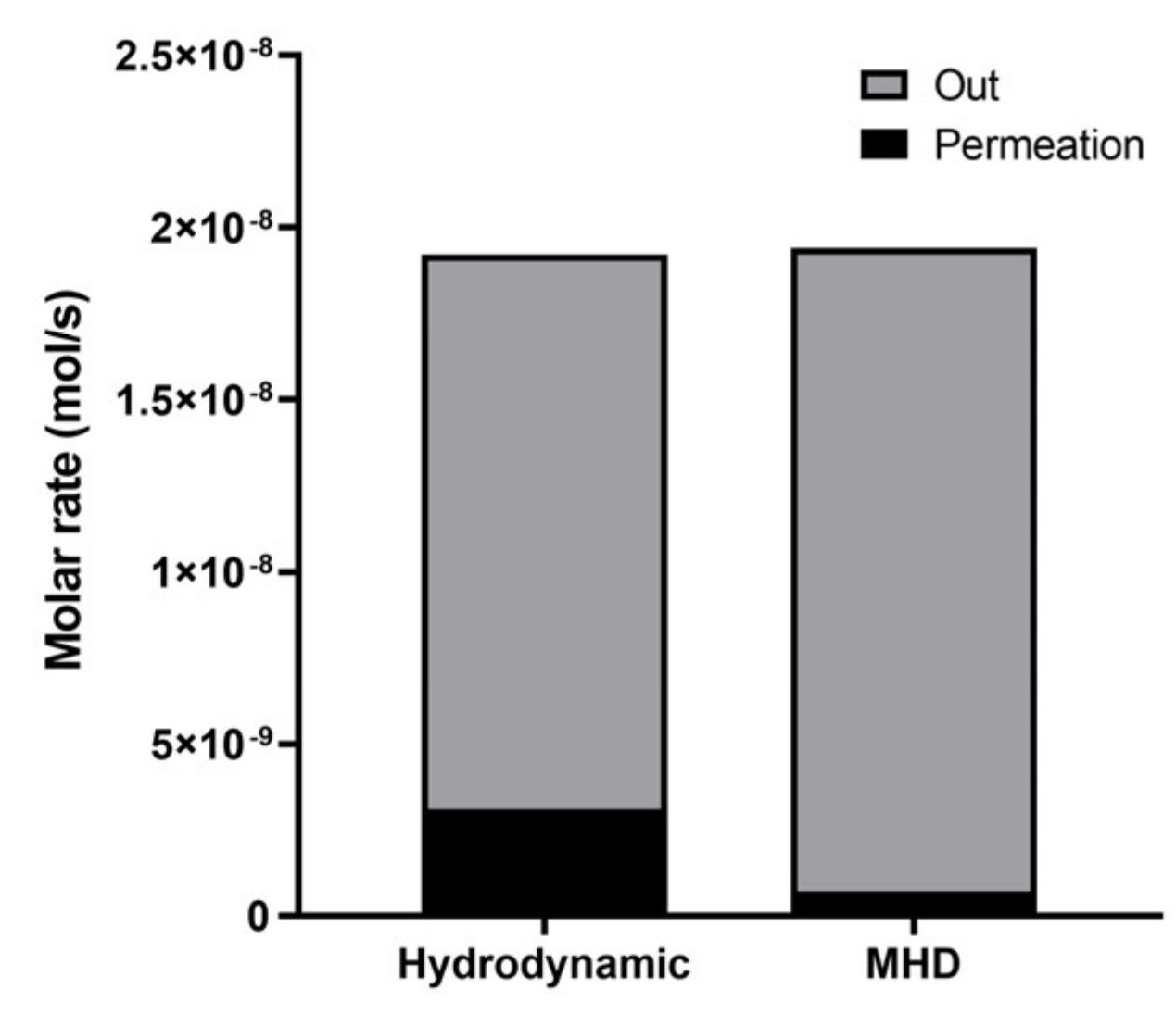
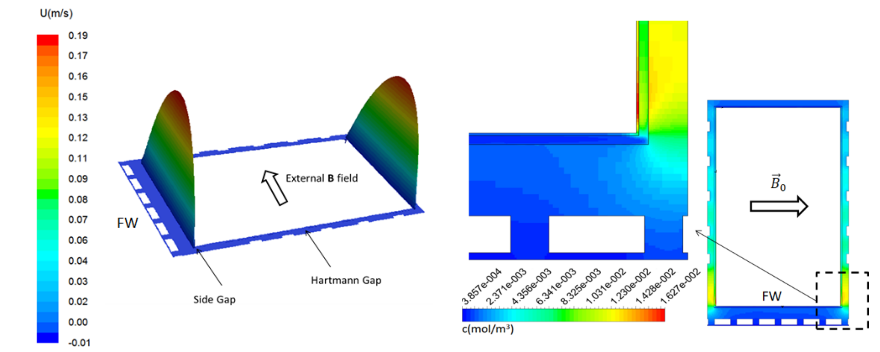