Self-Learning Pipeline for Low-Energy Resource-Constrained Devices

Abstract

The trend of bringing machine learning (ML) to the Internet of Things (IoT) field devices is becoming ever more relevant, also reducing the overall energy need of the applications. ML models are usually trained in the cloud and then deployed on edge devices. Most IoT devices generate large amounts of unlabeled data, which are expensive and challenging to annotate. This paper introduces the self-learning autonomous edge learning and inferencing pipeline (AEP), deployable in a resource-constrained embedded system, which can be used for unsupervised local training and classification. AEP uses two complementary approaches: pseudo-label generation with a confidence measure using k-means clustering and periodic training of one of the supported classifiers, namely decision tree (DT) and k-nearest neighbor (k-NN), exploiting the pseudo-labels. We tested the proposed system on two IoT datasets. The AEP, running on the STM NUCLEO-H743ZI2 microcontroller, achieves comparable accuracy levels as same-type models trained on actual labels. The paper makes an in-depth performance analysis of the system, particularly addressing the limited memory footprint of embedded devices and the need to support remote training robustness.

1. Introduction

Maturation of machine learning (ML) is enabling embedding intelligence in Internet of Things (IoT) devices [1]. Various effective machine and deep learning models have been deployed on resource-constrained devices to gain insights from collected data. Field devices, such as microcontrollers, consume significantly less energy than larger devices, especially if their memory footprint is minimized and huge edge-cloud raw data transmission can be spared by only sending high-level information.

Typically, ML models are trained on high-performance computers in the cloud and then deployed on IoT devices to perform the target inference task. However, in real-world applications, statically trained models are not able to adapt to the environment, which could reduce accuracy for new samples. Training a ML model on the device, instead, has the ability to learn from the physical world and update the system locally. This allows for lifelong incremental learning [2] updating its knowledge, as well as personalizing the device thus improving performance by learning the characteristics of the specific deployment context.

Moreover, as millions of new IoT devices are produced every year [3], vast amounts of unlabeled data in various domains (e.g., industrial, healthcare, environmental, etc.) are generated. Designing systems based solely on supervised learning, which requires a labeled dataset, is not ideal for IoT scenarios. Creating labeled IoT datasets is expensive and hardly feasible [4]. Therefore, it is of utmost importance to smartly leverage the quantity of unlabeled data produced by the end devices deployed in the field.

Semi-supervised and self-supervised learning techniques have shown encouraging results in learning from unlabeled data. The former approach exploits a partially labeled dataset [5], while the latter trains a model using automatically generated pseudo-labels [6,7]. Fully automated solutions look particularly suited for applications deployable in hostile environments, possibly due to difficulties in communications or the need to keep energy consumption and/or costs low. Target applications may involve, for instance, remote agriculture, farming, mining, manufacturing, emergency, or the military.

We have explored feasibility of a self-supervised learning system in an embedded environment in [7]. In this new paper, we are interested in going more in depth with the performance analysis, also tackling three research questions. First, we investigate the possibility of increasing robustness in a sample selection for automated training, as the training data in such an autonomous system should be as compact and noiseless as possible to avoid performance degradation. We are interested in sample selection rather than feature selection (which is another method of dataset reduction), as we assume that the sensor configuration of a device deployed in the field is already optimized according to the target application. Second, we investigate the possible advantages of a memory management algorithm for limited resource field devices to minimize the memory occupation associated with the continuous flow of samples that may be used for the training set. Third, we perform a timing analysis on a state-of-the-art microcontroller to evaluate the overall system’s ability to meet real-time performance requirements.

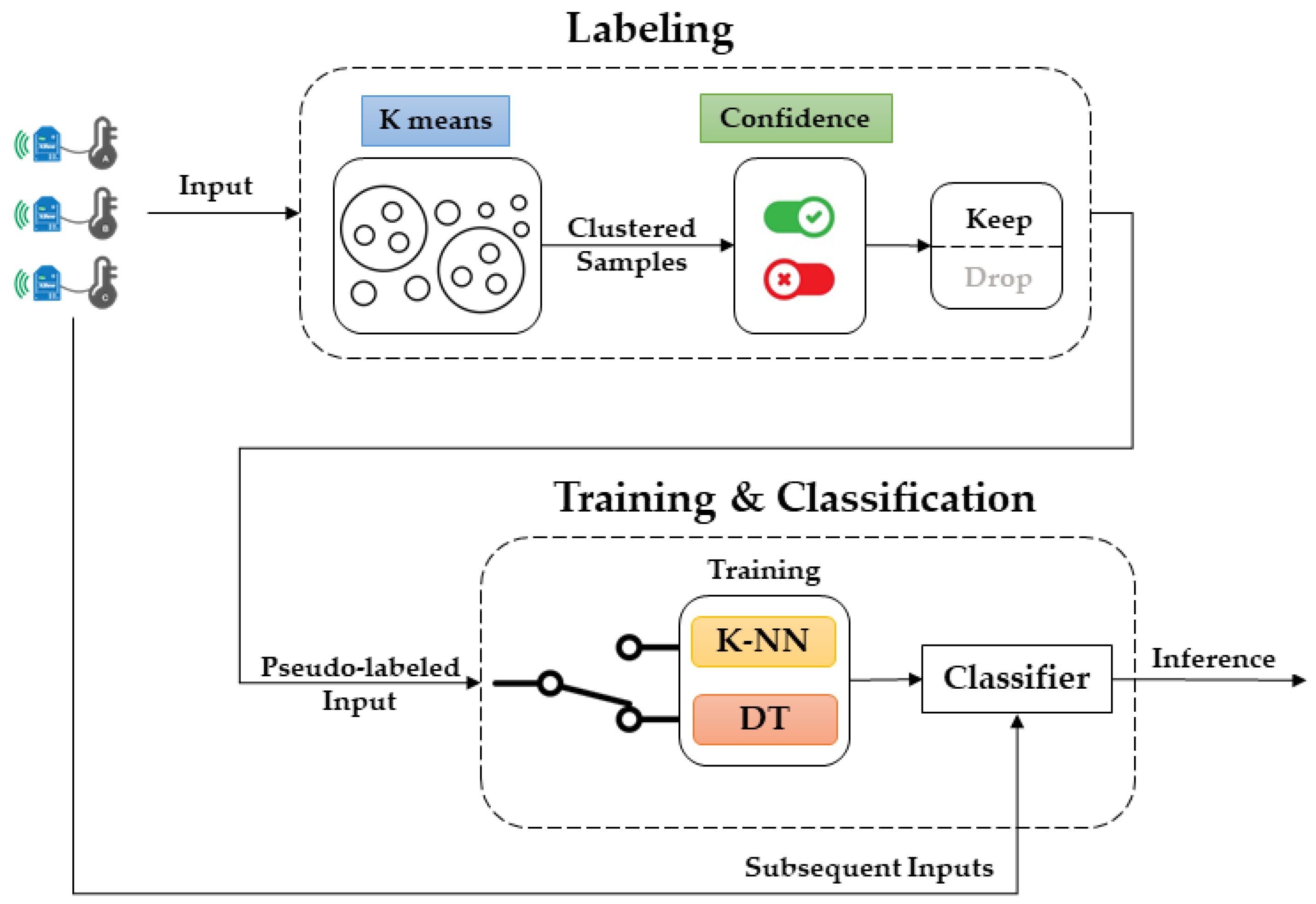
We have performed this analysis on the Self-Learning Autonomous Edge Learning and Inferencing Pipeline (AEP) system. AEP is a software system we have developed for resource-constrained devices. Besides the inference capability, the AEP allows autonomous field training by means of a two-stage pipeline, involving a label generation with a confidence measure step and on-device training. This paper presents an in-depth evaluation of the proposed system on two publicly available datasets for IoT applications, using the NUCLEO-H743ZI2 microcontroller.

The remainder of this paper is organized as follows: Section 2 reviews related work, and Section 3 provides some background on the algorithms employed in the pipeline. Section 4 presents the proposed system, and Section 5 the experimental analysis. Section 6 concludes the paper and indicates possible directions for future research.

2. Literature Review

A large research effort has been devoted to learning from unlabeled data. We can identify three main research areas in the field: combining clustering with classification, semi-supervised learning, and self-supervised learning, as shown in this section.

2.1. Combining Supervised and Unsupervised Learning

Qaddoura et al. [8] propose a three-stage classification approach for IoT intrusion detection. In the first stage, the IoT training data is reduced by 10% after grouping the data using k-means clustering. Then, oversampling is performed to address the lack of minority class instances. In the final stage, the enlarged dataset is used to train a single hidden layer feed-forward neural network. The authors claim that the proposed approach outperforms other approaches on the selected dataset. Reference [9] proposes a method to improve the classification accuracy by applying clustering techniques, namely k-means and hierarchical clustering, to the dataset before the classification algorithms. Their experimental analysis shows that higher accuracy is achieved after applying the classification algorithms, namely naïve Bayes and neural network, to the clustered data. The work in [10] presents a hybrid framework that uses network traffic to protect IoT networks from unauthorized device access. For each device type in the dataset, a binary one-vs-rest random forest classifier is trained, and the model is stored. During prediction, if all saved classifiers failed to classify the feature vector as a “known” device, the OPTICS clustering algorithm is used to group devices with similar behavior together. Experimental results on ten IoT device types (three types are provided without labels) show good accuracy levels, and reduced runtime and memory requirements due to the use of an autoencoder. Reference [7] proposes an autonomous edge learning and inferencing pipeline with a k-NN classifier, which is periodically trained with the labels obtained from clustering the dataset via k-means. This embedded system performs only slightly worse than manually labeled k-means in terms of accuracy, particularly with small data subsets.

2.2. Semi-Supervised Learning

Semi-supervised approaches refer to training a specific classifier using a small amount of annotated data in conjunction with a large amount of unlabeled data [5]. The general workflow first consists of training a classifier using the small set of labeled training data. Then, the classifier is used to predict the outputs (pseudo-labels) of the unlabeled data. The final step is to train the model on the labeled and pseudo-labeled data.

In [11], Zhou et al. designed a semi-supervised deep learning framework for human activity detection in IoT. The proposed method exploits two modules. The auto-labeling module is based on reinforcement learning and assigns labels to the input data before sending it to the LSTM-based classification module for training. The evaluation of the framework shows the effectiveness of the proposed method in the case of weakly labeled data (i.e., large amount of unlabeled data and a small amount of labeled data). Ravi and Shalinie [12] propose a mechanism for distributed denial of service (DDoS) mitigation and detection based on an extreme learning machine algorithm trained in a semi-supervised manner. They demonstrate the effectiveness of the proposed approach compared to other ML algorithms. Rathore et al. [13] propose a fog-based framework that integrates a semi-supervised fuzzy c-means with an extreme learning machine classifier for efficient attack detection in IoT. The proposed framework achieves better performance and detection time when compared to cloud-based attack detection frameworks.

2.3. Self-Supervised Learning

The idea behind self-supervision is to find a surrogate task for the network to learn that does not require explicit labeling, but rather the inherent structure of the data that provides the labels. Self-supervised learning is a branch of unsupervised training in which pseudo-labels are automatically generated from the data itself [6]; then, a model is trained through supervised learning exploiting such pseudo-labels (e.g., [14]).

In this area, Wu et al. [15] propose a framework for on-device training of convolutional neural networks that consists of two approaches: a self-supervised early instance filtering of the data to select important samples from the input stream, and an error-map pruning algorithm to drop insignificant computations in the backward pass. The framework reduces the computational and energy costs of training with little loss of accuracy. Human activity detection with self-supervised learning is introduced in [16]. Signal transformation is performed as a pretext task for label generation and various activity recognition tasks are performed on six public datasets. The results show that self-supervised learning enables the convolutional model to learn high-level features. Saeed et al. [17] present a self-supervised method that learns representations from unlabeled multisensory data based on wavelet transform. The approach is evaluated on the datasets with sensory streams and achieves comparable performance to fully supervised networks.

2.4. IoT Infrastructure and Data

The Internet of Things refers to billions of devices connected to the Internet, which collect and share data from the field [18]. Typical IoT architectures consist of a set of technological layers, bringing scalability, modularity, and configurability (e.g., [19,20]). The first layer (namely, the perception layer) consists of smart objects equipped with sensors, such as fiber optic sensors (FOS), microelectromechanical systems (MEMS), sensors, radio frequency identification (RFID) sensors, etc. The second layer is the network layer. Current networks, often connected with very different protocols, have been deployed to support machine-to-machine (M2M) networks and their applications. There may be a local area network (LAN), such as Ethernet and Wi-Fi connections, or a personal area network (PAN) such as ZigBee, Bluetooth, and ultra wideband (UWB). Sensors that require low power and low data rate connectivity typically form networks commonly known as wireless sensor networks (WSNs). Besides the sensor aggregators, the connection to backend servers/applications in the cloud is made over wide area networks (WAN) such as GPRS, LTE, and 5G protocols that are widely used for IoT, including constrained application protocol (CoAP), message queuing telemetry transport (MQTT), extensible messaging and presence protocol (XMPP), etc. Finally, the application layer is responsible for delivering services to the user exploiting the IoT field data. This layer also includes data storage, management, and processing. The data management infrastructure includes common data stores, such as relational or non-relational databases, distributed file systems, such as the hadoop distributed file system (HDFS), etc. The data processing techniques are generally based on machine learning or artificial intelligence and pattern recognition algorithms.

The overall application latency is typically dominated by the propagation delay between the edge and the data centers on the cloud. Another significant performance penalty factor is given by packet losses [21]. This, together with consideration about bandwidth, energy consumption, and privacy, suggests the importance of edge computing, thus keeping the computation as much as possible close to the information source [22].

Reference [23] singles out four main characteristics of IoT data in cloud platforms: multisource high heterogeneity, huge scale dynamic, low-level with weak semantics, and inaccuracy. These characteristics are important, as they highlight key features that should be provided by an effective IoT data framework (e.g., source characterization, variety of source data configurations/aggregation, outlier computation) [24].

IoT data characteristics are largely dependent on delay, incompletion, and dynamic variation.

3. Autonomous Edge Pipeline (AEP) Algorithms

Before presenting the AEP system architecture and the supported workflow, we give a short overview of the underlying algorithms. Particularly, we use k-means clustering for unsupervised learning, which provides the binary labels for training a decision tree or a k-NN classifier (supervised learning), which is used for the actual classification of the samples.

3.1. Unsupervised Learning

Unsupervised learning is a branch of ML that derives interesting patterns and insights directly from unlabeled datasets. Clustering consists of the unsupervised classification of (unlabeled) samples into groups or clusters such that data points in the same group are similar to each other and different from data points in other clusters [25].

In the AEP implementation, we use one of the most common clustering methods, namely k-means clustering. This algorithm works iteratively to partition a set of observations into k (predetermined) distinct and non-overlapping clusters based on feature similarity. It first selects k random data points as initial centroids. In the next step, each data sample is assigned to the closest centroid based on a certain proximity measure. Once all the data points are assigned and the clusters are formed, the centroids are updated with the mean of all the data samples belonging to the same cluster. The algorithm iteratively repeats these two steps until a convergence criterion is met [26]. One drawback of the standard k-means is its sensitivity to the initial placement of centroids. Therefore, our AEP implementation uses the k-means++ algorithm [27], which combines the standard k-means with a smarter initialization of the centroids. k-means++ first chooses a random point from the data as the first centroid. Then, for each instance in the dataset, k-means++ computes the distance to the nearest centroid previously selected. Then, it selects the next centroid from the remaining data points, such that it has the largest distance to the closest centroid previously selected. These steps are repeated until k centroids are chosen.

As we will see in Section 4.2 (“Development Challenges”), the AEP also exploits the soft k-means enhancement, which provides a confidence value when assigning samples to clusters, thus allowing an increase in robustness of the system.

3.2. Supervised Learning

Supervised learning is the most common branch of ML and is implemented by our AEP system to classify the samples based on the pseudo-labels generated through the unsupervised learning module. Supervised learning is the process of deriving a function that maps an input to an output, based on labeled training data. Each training example is a pair consisting of an input vector (features) and a desired output (class or value, for classification and regression, respectively) [28].

The AEP system currently features two supervised learning algorithms:

• k-nearest neighbor (k-NN) [29] is a non-parametric lazy-learner algorithm used for classification and regression. k-NN stores all the available dataset and classifies a new sample based on the feature similarity between this new case and the available data, assigning the most numerous class of the nearest k labeled points. The performance of this algorithm depends only on the number of neighbors N to be considered in each decision;
• Decision tree (DT) [30] is a well-established ML technique that belongs to the supervised learning family. As the name suggests, it uses a tree-like model of decisions. The training phase takes as input a training set and recursively partitions the samples into subsets to improve a “label” column purity score in each partition. The purity score is a method based on the proportion of each class in a mixture of class labels. The higher the proportion of one of the classes, the purer the subset.

We have selected these three algorithms (one for labelling and two alternative for classification), at least as an initial choice, keeping into account the limitations on memory and computational resources of the targeted edge devices [31]. The k-means method is efficient with guaranteed convergence, and fast when running on small processors with low capabilities [26]. k-NN is a simple algorithm with good performance and requires no training [29]. Finally, DTs require little to no data preprocessing effort and can effectively handle missing values in the data [30].

4. Autonomous Edge Pipeline (AEP)

4.1. Framework Overview

The self-learning AEP (Figure 1) is an iterative pipeline that alternates between clustering/training and classification. Particularly, k-means clustering is periodically executed on the input stream and provides the pseudo-labeled clustered data. The labeling results are then evaluated by a confidence algorithm (if enabled by the user), presented in Section 4.2, which makes a binary decision whether to keep or discard each instance. Once important samples with their corresponding pseudo-labels are selected, the training process is executed (this applies to the DT case only, since k-NN does not involve a training phase). The resulting classifier then continuously classifies the incoming samples. Given the resource limitations of the target devices, a memory management strategy is implemented to prevent memory overflow, which is explained in the following subsection.

4.2. Development Challenges

In the following, we discuss the main challenges we faced in developing the AEP system: filtering of samples to be used for the training; dataset management on the edge and DT training on the edge.

• Filtering of samples to be used for the training. k-means is a hard clustering algorithm, as the data points are assigned exclusively to one cluster. However, in some situations (e.g., in our case in which clustering is used to define labels to train a classifier), it is important to find out how confident the algorithm is in each one of its decisions. The soft k-means improvement calculates a weight that determines the extent to which each data sample belongs to each cluster [26]. Higher values indicate a certain or strong assignment, and lower weights indicate a weak assignment. The soft k-means weights can also be computed a posteriori, using cluster centers obtained by a hard k-means, exploiting Equation (1):

$$w_{ij}=\frac{1}{{{\displaystyle \sum }}_{k=1}^c{\left(\frac{\parallel x_i-c_j\parallel }{\parallel x_i-c_k\parallel }\right)}^{\frac{2}{m-1}}},$$

(1)

where x_i is a data point, c_j is the coordinates of the jth cluster center, and m is a parameter that controls the fuzziness of the algorithm, typically set to 2 [26]. Once the soft k-means weights for each sample are computed (using the Euclidean distance), a confidence threshold can be set (e.g., with a value of 0.9), so to remove all samples that cannot be assigned to a cluster with a higher weight than the threshold. This approach is beneficial in terms of removing outliers or data points in uncertain regions, and can improve clustering results and overall system performance, particularly robustness;

• Dataset memory management on the edge. In resource-constrained scenarios, there is a need to manage the amount of data to prevent memory overflow caused by continuous sampling and consequent increase in the training set. Additionally, the k-NN algorithm is also very memory hungry as it needs to store the entire training set for the inference phase. To tackle these challenges, we implemented three memory management algorithms: first in, first out (FIFO), which removes the older samples, when the memory is full; random memory filtering (RND); and CONF memory filtering, which retains in memory samples having higher confidence values. The impact on performance of these memory management strategies is compared in the experimental analysis section.
• Training the decision tree on the edge. The DT training algorithm used in the AEP is implemented from scratch in C language, as we could not find a publicly available version for Cortex-M microcontrollers. The implemented training algorithm is classification and regression trees (CART), which constructs binary trees using the features and thresholds that yield the largest information gain at each node [32]. Our implementation allows the user to specify two hyper-parameters for tree configuration, maximum depth of the tree, and a minimum number of samples required to split an internal node. To simplify the implementation on the target device, we implemented only the “Gini” splitting criterion, which is less computationally intensive than the entropy criterion.

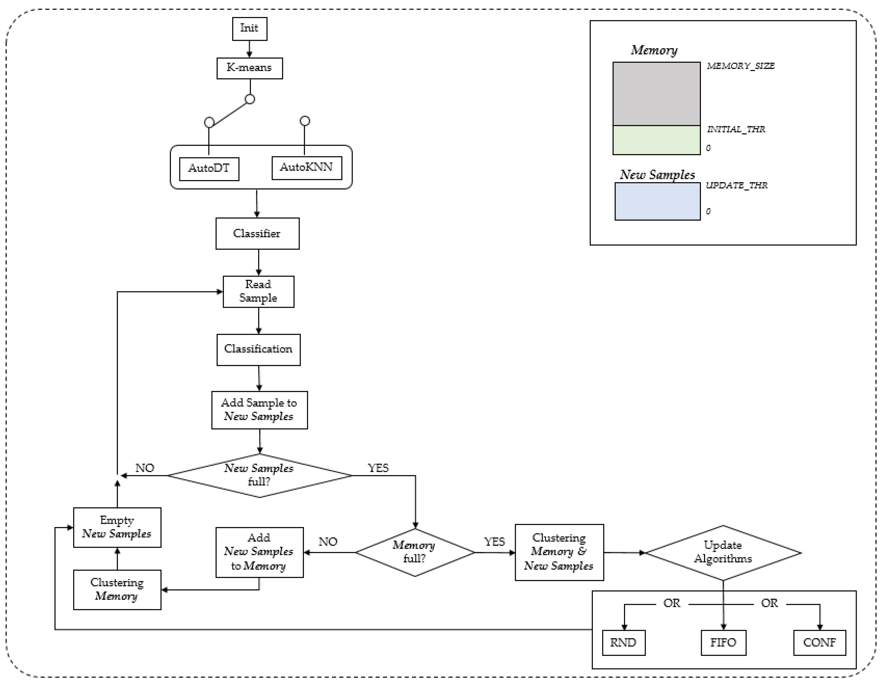
4.3. AEP Workflow and Memory Management

The workflow supported by the AEP is sketched in Figure 2. In the picture, the term AutoDT refers to a decision tree classifier trained on the pseudo-labeled data (obtained by the k-means clustering algorithm running on the field device). Similarly, AutoKNN is the alternative k-NN classifier, which requires no training but directly exploits the pseudo-labeled input dataset.

At start-up, the AEP has no knowledge nor data. The initial phase thus consists of filling the memory with data samples up to a user-specified initial threshold (i.e., INITIAL_THR). Once the threshold is reached, the k-means clustering is run on the recorded samples and returns their pseudo-labels. If the user sets the AutoDT option, the DT training algorithm is executed. As anticipated, the user can set the max tree-depth and min split-samples hyper-parameters for this algorithm. On the other hand, if AutoKNN is selected, the collected samples together with their corresponding pseudo-labels are ready to be used by the k-NN classifier, and the only user-selectable hyper-parameter is the number of neighbors, N.

After this start-up, the operation loop can begin. The trained model is used to classify the subsequent sample stream. In order to improve (or adapt) the classifier performance, the new samples can also be stored in a dedicated memory section called “New Samples” until an update threshold specified by the user is reached (e.g., UPDATE_THR). Then, k-means clustering is performed again for all samples in memory, providing the new set of pseudo-labels and updating the classifier accordingly. If the memory is full, one of the three data filtering algorithms available (i.e., RND, FIFO, or CONF—cfr. Previous sub-section) is run in order to prevent memory overflow. We should emphasize that the samples are considered independent and identically distributed (iid). In machine learning theory, the iid assumption is made for datasets to imply that all their samples have the same probability distribution and are mutually independent (e.g., the data distribution does not change over time or space).

The AEP is written in platform-independent C language (i.e., it does not use native OS libraries), which enables code mobility across different platforms. The proposed pipeline is integrated with the edge learning machine (ELM) framework [33,34] and can be used also on various types of microcontrollers and resource-constrained devices.

5. Experimental Analysis and Results

The experimental analysis was performed using a NUCLEO-H743ZI2 board with an Arm Cortex-M7 core running at 480 MHz, with 2 MB flash memory and 1 MB SRAM. The STM32 H7 series is a family of high performance microcontrollers offering higher security and multimedia features [35].

To characterize the performance of the AEP, we selected two binary classification datasets representing major IoT domains, such as health and industry. The first one is the well-known Pima Indians Diabetes Database (768 samples × 8 features), used for diabetes detection and prediction based on diagnostic measurements [36]. The second one is the semiconductor manufacturing process data (SECOM) (1567 × 590), which consists of signals generated from the semiconductor device to detect anomalies [37]. We chose two datasets from very different application domains in order to assess the proposed system in a significant range of field data typologies.

To make the datasets fit into the MCU memory and mimic a field device environment, we reduced both the datasets to only four features by applying feature selection using the scikit-learn library f_classif [38]. f_classif is used only for categorical targets and based on the analysis of variance (ANOVA) statistical test. To evaluate the effect of this dataset feature reduction (DFR), we tested the performance (accuracy) on the selected datasets of the two classifiers used in this work, namely DT and k-NN, before and after DFR, as shown in

Table 1. Classifiers’ performance (accuracy) before and after DFR.

Dataset	DT		k-NN
	Original	After DFR	Original	After DFR
Diabetes	85.0%	81.2%	83.1%	77.9%
SECOM	94.3%	92.2%	95.8%	92.2%

. We emphasize that the results in Table 1 are also the comparison reference for the various AEP implementations we will analyze later. Scikit-learn exhaustive grid search cross-validation [39] was used to select the best hyper-parameter values. In all experiments, the accuracy is measured with the same 20% test set.

The results show a 3% and 5% performance decrease in the diabetes dataset for DT and k-NN, respectively, while a 2% and 3% decrease was observed in SECOM. We thus argue that the applied DFR does not significantly affect the classifiers’ performance, and the resulting datasets can be used to evaluate the proposed AEP. Of course, in the AEP experiments, we did not use the actual labels in the training phase, but only as ground truth for comparing the classification results.

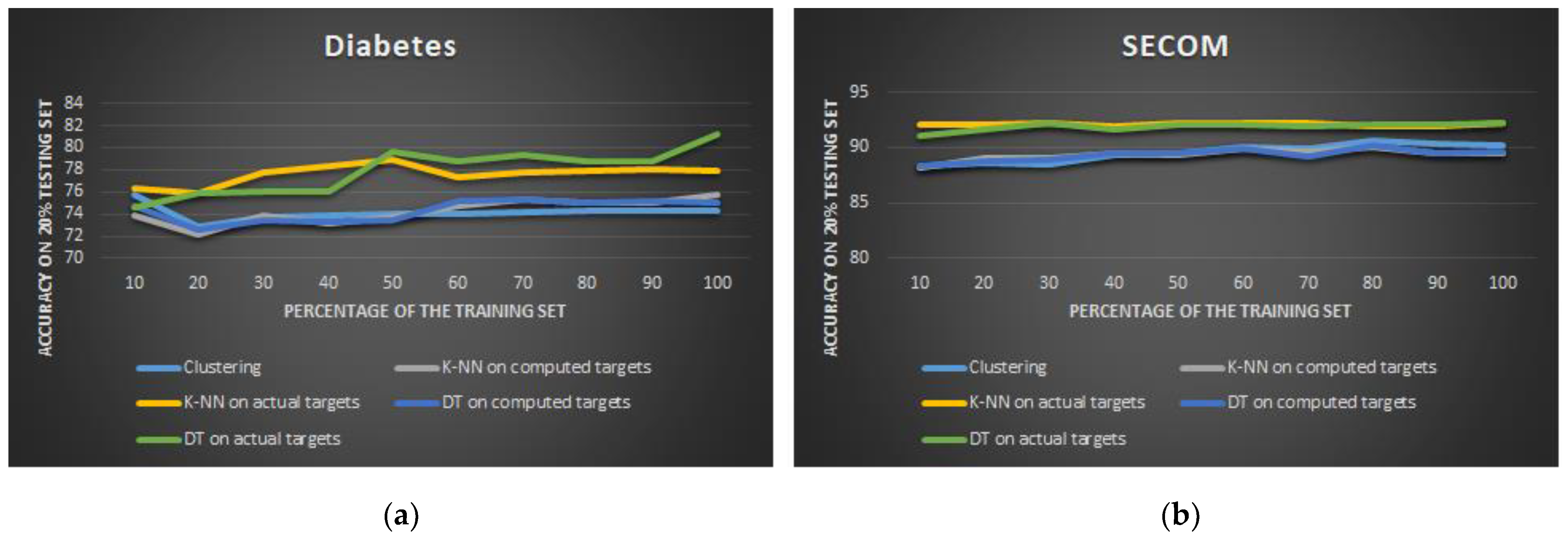
5.1. Learning Curves

Learning curves (LCs) are a commonly used diagnostic tool in ML for algorithms that learn incrementally from a training dataset, such as, in our case, described in Section 4.3. Learning curves are used to represent the predictive generalization performance as a function of the number of training samples. It is a visualization technique that can show how much a model benefits from adding more training examples [40].

As a first step, for each dataset, Figure 3 plots the learning curves for the two classifiers trained on the pseudo-labels obtained by k-means clustering (namely, AutoDT and AutoKNN), as a function of the size of the training set, which varies from 10% to 100% (out of the whole 80% training set size). For comparison, we also present the performance of the two classifiers trained on actual labels (DT and k-NN), as well as the performance of the k-means clustering only (clustering).

In Figure 3, we can see that, for the diabetes and SECOM datasets, the AEP (AutoDT and AutoKNN) is able to achieve accuracy levels comparable to the models of the same type (DT and k-NN) trained on actual labels. Performance of the SECOM dataset quickly saturates with a small percentage of training data. The “Clustering” approach almost always had similar accuracy levels as AEP. This is reasonable, as the latter exploits the labels generated by the k-means clustering algorithm to train its classifiers in the field.

AEP generally achieves fairly similar performance to the original supervised approach trained with actual labels (DT and KNN on actual labels). However, AEP has limitations, as the data in high-density areas affects the k-means clustering performance.

In the following subsections, we go more in depth with the analysis of the AEP, considering the three research questions reported in the introduction, analyzing the various steps and alternatives of the workflow described in Section 4.3.

5.2. Robustness in Sample Selection for Automated Training

The first research question investigates the possibility of making a self-supervised learning system robust in sample selection for automated training in the field. We thus explore the effect of not including in the training memory samples having a low confidence value, which is obtainable from the soft k-means algorithm.

5.2.1. AEP: AutoDT on the NUCLEO-H743ZI2

We evaluated the AEP with and without the confidence feature of the soft k-means algorithm (Section 4.2), with a confidence threshold of 0.9. We empirically identified this value as a good trade-off after several tests. A lower threshold means that more samples are retained, increasing the likelihood that points are in an uncertain (or dense) region, thus reducing the label robustness, while higher values may cause some representative data points to be discarded. In order to keep into account the memory limitations, we use the RND filtering strategy. For the performance analysis on the target device, we set the memory threshold values (MEMORY_SIZE, INITIAL_THR, and UPDATE_THR) to 200, 50, and 100 data samples, respectively. The best hyper-parameters for the AutoDT classifier are reported in

Table 2. Decision tree training hyper-parameters for the AutoDT.

Dataset	Max Depth	Min Samples
Diabetes	3	10
SECOM	2	10

, after multiple tests on the AEP. The learning curves for AutoDT are shown in Figure 4.

As described in the workflow in Section 4.3, the AEP starts learning incrementally until it reaches the MEMORY_SIZE threshold (200). At this point, the filtering strategy starts executing and the AEP is then only trained on MEMORY_SIZE samples.

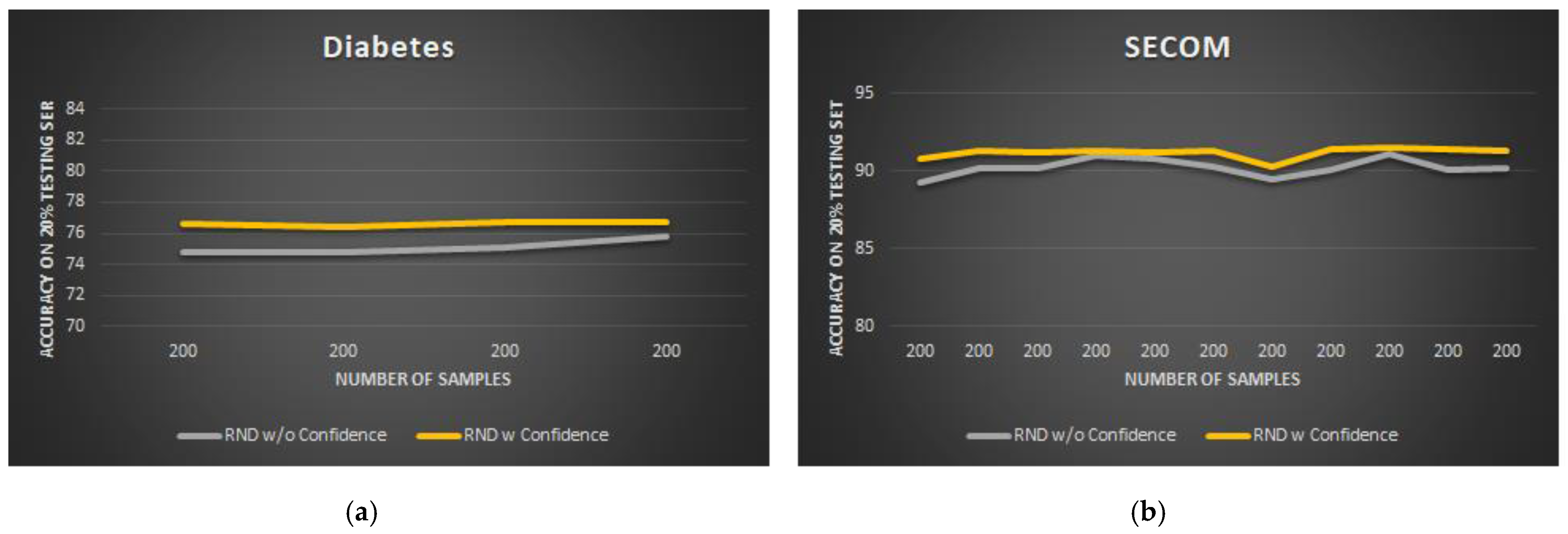
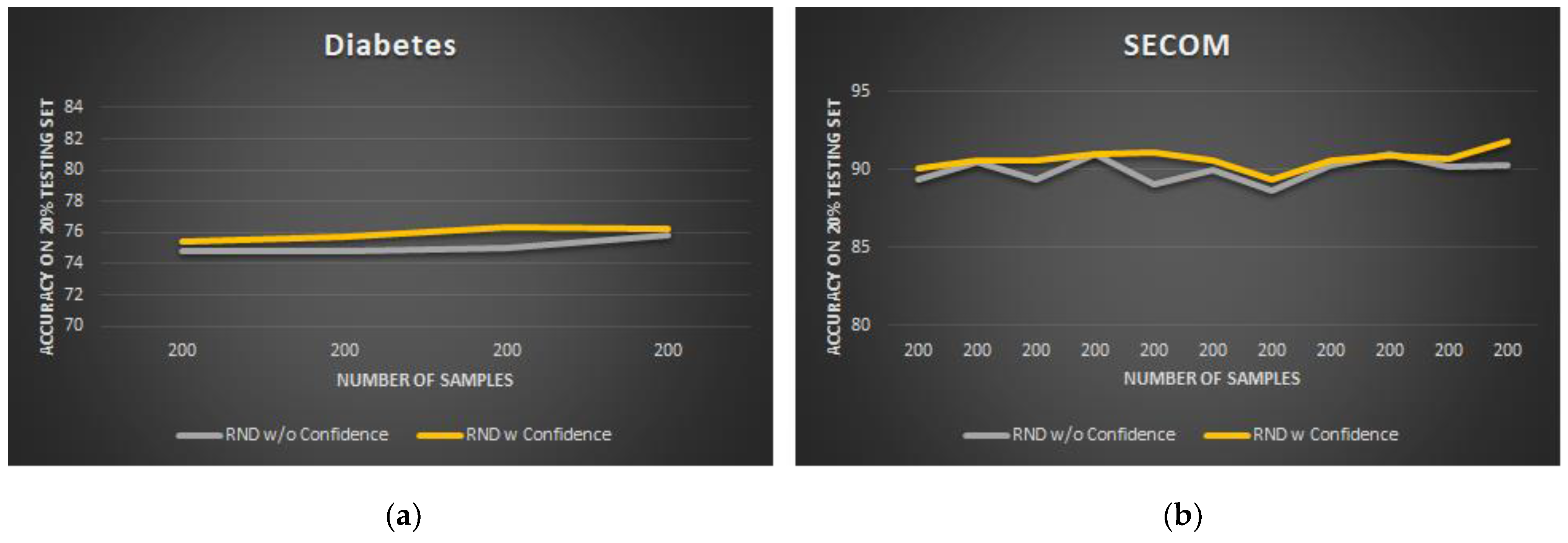
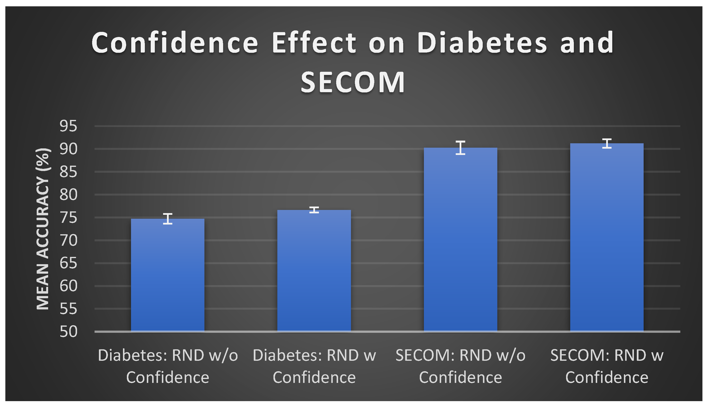
Overall, the learning curves in Figure 4 show that the Confidence algorithm leads to a certain accuracy increase in both the datasets (+1.9% for diabetes, +1.0% for SECOM). For better result presentation, the bar graphs in Figure 5 show the average accuracy and standard deviation of AutoDT on both the datasets in the MEMORY_SIZE occupation level case.

When we compare the above results with the DT classifier from Table 1 (after DFR), we can observe the following:

• Diabetes: the AutoDT model with confidence enabled achieves a 76.6% average accuracy, compared to 81.2% of the baseline DT model.
• SECOM: the AutoDT model with confidence achieves a 91.2% average accuracy compared to 92.2% of the baseline DT model.

5.2.2. AEP: AutoKNN on the NUCLEO-H743ZI2

For the memory part, the procedure for the AutoKNN case is the same as for AutoDT, which is described in the previous sub-section. The best hyper-parameter values for the AutoKNN classifier are reported in

Table 3. Number of neighbors for the AutoKNN.

Dataset	N Neighbors
Diabetes	5
SECOM	5

, after multiple tests on the AEP. The learning curves for AutoKNN are reported in Figure 6.

Overall, the AutoKNN learning curves for the diabetes and SECOM datasets show a limited improvement introduced by enabling the soft k-means confidence algorithm (+0.8% for diabetes, +0.7% for SECOM), but it should be noted that embedded performance is close to the reference desktop implementation (Table 1). To better illustrate the results, Figure 7 shows the mean accuracy and standard deviation of AutoKNN on the test datasets in the MEMORY_SIZE occupation level case.

Comparing the bar charts result with the baseline k-NN classifier from Table 1 (after DFR), we can observe the following:

• Diabetes: AutoKNN with confidence achieves a 76.07% average accuracy compared to 78.0% of the baseline k-NN model.
• SECOM: AutoKNN with confidence achieves a 90.7% average accuracy compared to 92.2% of baseline k-NN model.

5.3. Effect of Memory Management

In this section, we address the second research question, by comparing performance of the three implemented memory filtering strategies, namely RAND, FIFO, and CONF. Given the iid nature of our test dataset samples, we expect that the results of the RND and FIFO strategies should be very similar. An improvement is expected with the CONF strategy, since it should incrementally improve the dataset by retaining the samples with higher confidence values.

5.3.1. AEP: AutoDT on the NUCLEO-H743ZI2

The procedure for this analysis step is the same as for the first research question. As an additional comparison term, we compare the memory filtering strategies with a “one-shot” implementation of the AEP, where clustering and training are performed only the first time the threshold MEMORY_SIZE samples (200 samples in this case) is reached, without any further update of the classifier. Given its added value, soft k-means confidence thresholding is enabled in all the reported test cases, except for the one-shot scenario (as samples are never removed in this case). 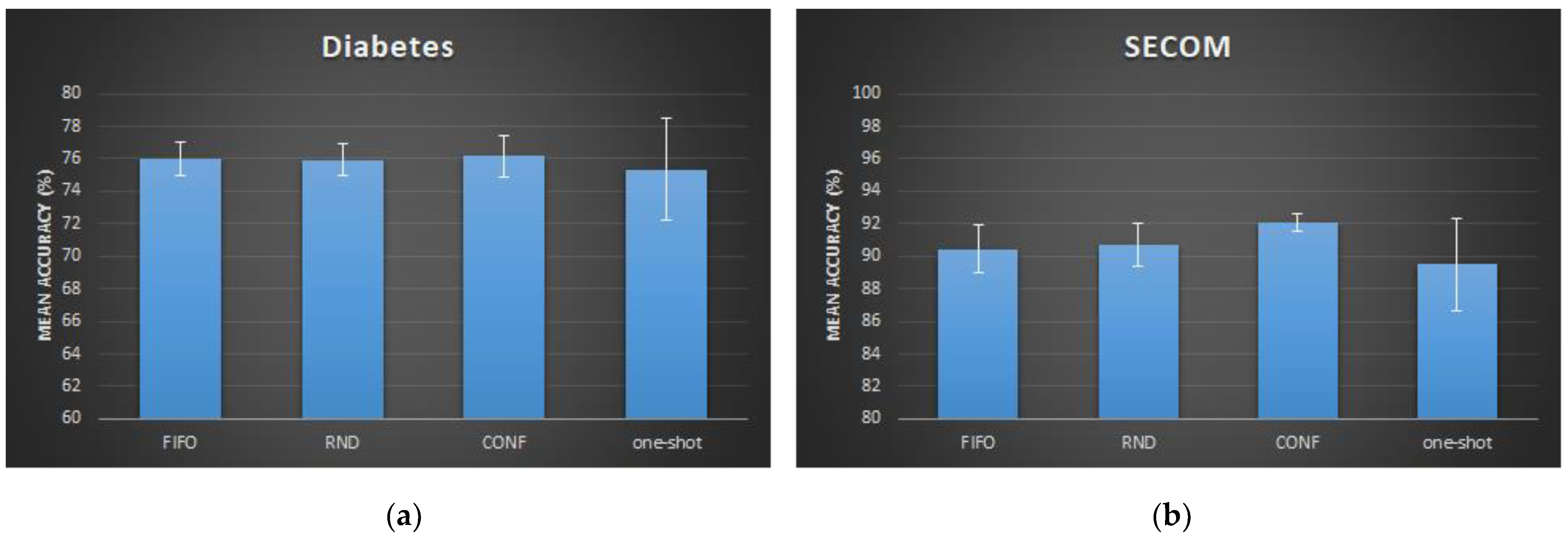Results are shown in the bar graphs in Figure 8.

Observing the bar chart results, we can see that the three filtering strategies have a similar accuracy for the diabetes dataset, with the CONF approach being slightly superior. However, the “one-shot” implementation had the lowest accuracy, because the confidence algorithm is disabled, and only the first MEMORY_SIZE samples are used. Additionally, for the SECOM dataset, the CONF memory filtering had the highest accuracy level, and the “one-shot” approach had the lowest one.

Comparing the above results with the baseline DT classifiers from Table 1 (after DFR), we can observe the following:

• Diabetes: the AutoDT model with CONF memory filtering and confidence enabled achieves a 76.7% average accuracy, compared to 81.2% of the baseline DT model.
• SECOM: the AutoDT model with CONF memory filtering and confidence enabled with 91.8% average accuracy, compared to 92.2% of the baseline decision tree model.

5.3.2. AEP: AutoKNN on the NUCLEO-H743ZI2

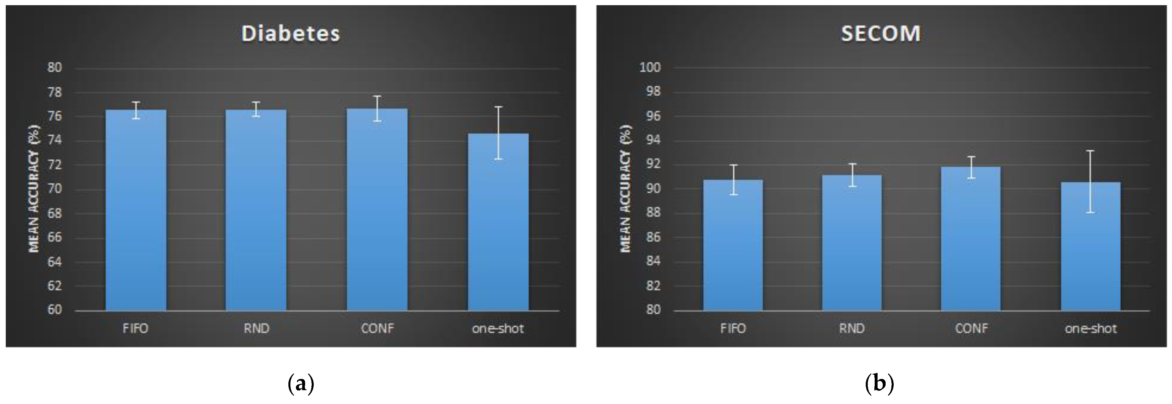
The same procedures as for AutoDT were applied for performance assessment of the AutoKNN module as well. The resulting bar charts are shown in Figure 9:

For the diabetes dataset, the three filtering strategies had an approximately equal accuracy levels with a slight superiority of the CONF strategy. Again, the “one-shot” implementation showed the lowest accuracy due to confidence disabling. The effect of the CONF filtering strategy is more pronounced in the SECOM dataset, with about 2% higher accuracy.

Comparing the bar chart result with the baseline k-NN classifiers from Table 1 (after DFR), we can observe the following:

• Diabetes: the AutoKNN model with CONF memory filtering and confidence enabled reaches a 76.2% average accuracy, compared to 77.9% of the baseline k-NN model.
• SECOM: the AutoKNN model with CONF memory filtering and confidence enabled reaches an 92.1% average accuracy, compared to 92.2% of the baseline k-NN model.

Similar to AutoDT results, the CONF strategy had the highest accuracy levels for both datasets.

5.4. Timing Performance Analysis

In the following subsections, we address the third research question by analyzing the timing performance of each AEP component (e.g., clustering, filtering, training, and classification) on the NUCLEO-H743ZI2 MCU running at 480 MHz (max).

5.4.1. k-Means Clustering Time

Table 4. k-means clustering time performance on the edge device with confidence algorithm enabled.

Dataset	Clustering Time (ms)
	Number of Samples
	50				150				200
	Min	Mean	Max	Stdev	Min	Mean	Max	Stdev	Min	Mean	Max	Stdev
Diabetes	52	52.6	53	0.6	156	156.6	157	0.6	261	300.5	315	26.1
SECOM	52	53.0	54	1	158	159.3	161	1.5	262	314.8	327	16.7

and

Table 5. k-means clustering time performance on the edge device with confidence algorithm disabled.

Dataset	Clustering Time (ms)
	Number of Samples
	50				150				200
	Min	Mean	Max	Stdev	Min	Mean	Max	Stdev	Min	Mean	Max	Stdev
Diabetes	52	52.0	52	0.0	143	148.0	152	4.6	220	288.9	319	43.5
SECOM	50	52.0	54	2.0	157	158.3	160	1.5	262	312.2	324	15.8

show the timing performance for the k-means clustering module of the AEP on the datasets with and without confidence algorithm enabled, respectively. This latency is important because it periodically affects the inference process, which is stopped (assuming a single-thread system) in order for the classifier to get the updated pseudo-labels.

The AEP first performs clustering on 50 samples and then, repeatedly, on 200 filtered samples (see Section 4.3). We thus report minimum, maximum, average, and standard deviation (three different runs under the same operating conditions) in the cases of: 50 samples (INITIAL_THR), 150 samples (INITIAL_THR + UPDATE_THR), and 200 samples, which represents the steady state condition and the most critical case (also because clustering and training with fewer samples happens only at the beginning of the operation). The minimum time for clustering given in Table 4 and Table 5 is achieved in the case of 50 samples, and the maximum time is achieved in the case of 200 samples. The comparison between Table 4 and Table 5 shows that enabling confidence results in slower clustering, which is due to the computational overhead (running the confidence algorithm on the clustering results).

Moreover, slight variations in the clustering time occurred due to the stopping criterion of the k-means clustering adopted in the AEP, which stops the algorithm once the centroids of the newly formed clusters stop changing. This criterion depends on the choice of the initial centroids, which affects the convergence speed. In all AEP tests, the maximum number of iterations of the k-means algorithm is set to 50 (the stopping criterion is met before this number in all tests).

5.4.2. Filtering Time

This latency is important, because filtering is performed at regular intervals and affects the inference process.

Table 6. Filtering time performance on the edge device with different strategies.

Datasets	Filtering Time (ms)
	FIFO w/o Confidence	FIFO w Confidence	RND w/o Confidence	RND w Confidence	CONF
Diabetes	1	<1	1	<1	9
SECOM	1	<1	1	<1	10

shows the timing performance for the three filtering strategies used in the AEP: FIFO, RND, and CONF.

The filtering is performed repeatedly to keep only MEMORY_SIZE samples (200 samples in this case). From the above results, for both datasets, we can see that FIFO and RND have the same timing performance, with a slightly faster filtering time when confidence is enabled. This is because the confidence algorithm removes some uncertain samples after clustering, resulting in a smaller number of samples that need to be filtered (e.g., instead of 200 out of 300 samples, 200 out of 280 samples would be filtered). The CONF strategy takes more time due to the execution of the sorting algorithm needed to identify the MEMORY_SIZE samples having higher confidence.

5.4.3. Decision Tree Training Time

Another significant AEP system latency factor is given by the DT training time, which is summed with the clustering time and filtering time discussed in the previous sub-sections. The results in

Table 7. Decision tree training time on the edge device.

Dataset	DT Training Time (ms)
	Number of Samples
	50				150				200
	Min	Mean	Max	Stdev	Min	Mean	Max	Stdev	Min	Mean	Max	Stdev
Diabetes	5	6.0	7	1.0	37	43.3	50	6.5	104	127.5	139	11.2
SECOM	10	10.6	11	0.6	86	90.6	94	4.2	71	133.3	198	36.5

illustrate the minimum, maximum, and average training latency on the datasets using the hyper-parameter configuration reported in Table 2.

While starting from an empty dataset, which is continuously updated, the training time varies with the number of samples, so three cases were considered: the case with 50 samples (INITIAL_THR samples), the case with 150 samples (INITIAL_THR + UPDATE_THR), and the case with 200 samples (steady state condition). Confidence is enabled in all cases, and the CONF filtering method is used for the 200 sample case (the temporal effects of the filtering strategies are analyzed in the previous section).

The minimum training time, reported in Table 7, is achieved in the 50 sample case, and the maximum time is achieved in the 200 sample case. The average AutoDT training time and standard deviation analysis are also shown in Table 7 after three different runs in the same operational conditions.

5.4.4. Inference Time:

The time for inference with the DT and the k-NN classifiers in the AEP is shown in

Table 8. Inference time performance on the edge device for the two supported classifiers.

Dataset	Inference Time (ms)
	DT	KNN
Diabetes	<1	1
SECOM	<1	1

. We always consider the 200 samples case, which is the steady-state condition.

The inference time with the DT classifier is relatively low (less than 1 ms) for both datasets. This is because the DT algorithm produces a simple model despite the size of the training set. For the k-NN classifier, the inference time is slightly higher (1 ms for both datasets), because the k-NN inference algorithm requires the exploration of the entire training set, and thus its size plays an important role in the timing performance.

5.5. AEP vs. Full Supervised Scenario on the Edge

As a final experiment, we compared the performance of the baseline models from Table 1 in a fully supervised scenario (i.e., training on the cloud then deploy the model) with the performance of AEP (accuracy and latency), and the results are shown in

Table 9. Performance evaluation between base models and AEP on the NUCLEO-H743ZI2 board.

Dataset	DT		AutoDT		k-NN		AutoKNN
	Accuracy	Inference Time	Accuracy	Inference Time	Accuracy	Inference Time	Accuracy	Inference Time
Diabetes	81.16%	<1 ms	76.67% (−5.53%)	<1 ms	77.90%	4 ms	76.17% (−0.22%)	1 ms
SECOM	92.22%	<1 ms	91.83% (−0.42%)	<1 ms	92.22%	7 ms	92.07% (−0.16%)	1 ms

. The base models are deployed with the Micro-LM module of the ELM framework [33].

From the results, we can see that the AEP accuracy drop wrt the baseline models is up to 5.5% and 0.4% for diabetes and SECOM, respectively. The inference time is relatively short in all cases, with partially better performance on the AEP (since fewer samples are processed, MEMORY_SIZE = 200 samples).

However, it is important to emphasize that the inference time performance reported in Table 8 does not take into account the specific case of the samples coming every UPDATE_THR samples (100 new samples in this case study), when a new clustering and training run is performed by the AEP. For such samples, the latency is thus given by Equations (2) and (3), for AutoDT and AutoKNN, respectively.

Table 10. Inference time for the first sample after each UPDATE_THR.

Dataset	Inference Time (ms)
	AutoDT	AutoKNN
Diabetes	437.2	310.7
SECOM	458.2	325.9

shows the computed inference time for this sample for both datasets:

$$AutoD{T}_{latency@UT}=inference\_tim{e}_{DT\_Table\_8}+ae{p}_{clustering\_time}+ae{p}_{filtering\_time}+ae{p}_{DT\_training\_time}$$

(2)

$$AutoKN{N}_{latency@UT}=inference tim{e}_{KNN\_Table\_8}+ae{p}_{clustering\_time}+ae{p}_{filtering time}$$

(3)

The “one-shot” AEP option avoids the periodical update, at the cost of an accuracy drop with respect to the full AEP system reported in Table 9. The comparison is provided in

Table 11. “One-shot” AEP performance accuracy (and accuracy drop with respect to the full AEP system) on the NUCLEO-H743ZI2 board.

Dataset	Accuracy		Accuracy Drop
	AutoDT	AutoKNN	AutoDT	AutoKNN
Diabetes	74.67%	75.32%	2.00%	0.85%
SECOM	90.58%	89.48%	1.25%	2.59%

. For the diabetes dataset, a 2% decrease in accuracy is observed when using AutoDT, while a marginal loss in accuracy of less than 1% is observed when using AutoKNN. For the SECOM dataset, a degradation in accuracy by 1.25% and 2.59% is observed for AutoDT and AutoKNN, respectively.

5.6. Summative Considerations

As a summary, we can state that the AEP (AutoDT and AutoKNN) provides accuracy levels comparable to the models of the same type (DT and KNN) trained on actual labels and with the full dataset. This stresses feasibility and effectiveness of the proposed self-learning pipeline. Our experience has also shown that not including in the training memory samples having a soft k-means confidence value under a certain threshold is a good option to enhance overall system robustness, especially in the case of overlapping clusters, and leads to performance improvement in all cases. Robustness—which is particularly critical in remote, autonomous systems—can be further increased by implementing a sample filtering strategy (e.g., CONF, which outperforms FIFO and RND), which allows us to incrementally improve the dataset (while not increasing its size) by retaining the samples with higher confidence values. In our tests, the achieved accuracy improvements are relatively limited (under 3%) but allow us to move closer to the reference values of the supervised learning implementation. We also argue that the test datasets are already optimized, while actual field operation may deal with noisy measurements, in which case the robustness enhancing solutions presented in this paper should be more relevant.

Considering the timing performance, the inference time is relatively low in all cases, but the overhead incurred by periodic clustering and training may be unacceptable in some real-time application cases due to the interruption of the usual (inference) flow. To avoid this temporal overhead, a simple “one-shot” execution implementation is available from the AEP at the cost of a slight decrease in accuracy. A better solution could be achieved by parallelizing the inference and clustering/training tasks in a real-time embedded operating system, provided that the inference task does not already consume the whole CPU time, if the system is not multi-core.

6. Conclusions and Future Work

With the rapid development of IoT technologies, end-devices deployed in the field are becoming ever more powerful and able to process data before delivery to the cloud, thus reducing transmission rates, bandwidth, and energy consumption. Processing data through ML models typically requires supervised training, which requires labeled datasets. Manual labelling of datasets is a bottleneck that is addressed in literature through development of semi-supervised learning and self-supervised learning techniques.

The advancement over state-of-the-art advancements aimed by this paper is twofold. First, we have proposed the autonomous edge pipeline (AEP), a system that combines unsupervised clustering, supervised learning, and inferencing in order to autonomously classify binary samples on the edge. The system is implemented in pure C, which makes it available for any microcontroller and resource constrained device. The system also features training memory management strategies in order to deal with the limited footprint of embedded devices and keep the energy demand low. To support the research activity in the field, the AEP is made available open source in the context of the ELM platform [33] (https://github.com/Edge-Learning-Machine/AEP (accessed on 16 September 2021)).

Second, we have explored the performance of the system in order to obtain a quantitative characterization of self-learning in an embedded environment. An experimental analysis of two publicly available IoT datasets shows that the AEP achieves similar performance levels as the corresponding models trained on actual labels and with the full dataset. Our experience stresses the importance of filtering some samples in order to select the most effective samples for building the training set. This can be achieved by setting a proper threshold for the confidence value provided by the soft k-means algorithm. Classification performance can be slightly increased over time by keeping in the training memory only the samples with higher confidence values, and periodically executing new training sessions. In terms of timing performance, the inference time is very short, but the overhead incurred by periodic clustering and training penalizes the timing performance. This extra time overhead can be avoided by a “one-shot” implementation, where clustering and training are performed only once when the threshold MEMORY_SIZE samples is reached, resulting in a slight drop in accuracy.

The AEP system is completely application independent. Potential benefits are expected to be significant in several application domains, for instance as it would allow introducing checks that are currently not foreseeable because of the need for manual sample labeling. For example, it could be possible to extend quality control in industrial plants by applying the AEP to detect defects and anomalies in several stages of a manufacturing chain. This application scenario is also close to the one represented by the SECOM dataset studied in this paper. Of course, the loss in accuracy wrt a supervised-learning-based system should be carefully considered in a complete system/product design perspective, particularly for health/safety-related applications, for which unsupervised learning looks critical. More generally, human factor aspects, such as privacy, invasiveness, and dignity, must be always taken into account when designing real-world applications.

In the future, we plan to extend the implementation of the AEP to support other labeling methods and classification algorithms, paying particular attention to the computational cost of the training phase, which could be particularly critical on resource-scarce devices and may require some optimizations. We are also interested in exploring an AEP extension addressing time-series. Moreover, task parallelism or an escape algorithm is required to avoid the inference latency overhead caused by the labeling and training phases needed at each model update.