Global Liquified Natural Gas Trade under Energy Transition

Abstract

With the recent rising attention and debates on the role of natural gas, especially liquid natural gas, in energy transition, it is critical to have a consistent approach in assessing uncertainties and dynamics in the global gas market during the next two to three decades. There are two objectives of this paper. The first one is to estimate and discuss the impacts of the global liquified natural gas (LNG) trade under a low-carbon scenario using a partial equilibrium model. The second objective is to discuss the role of a structural economic model in empirical analysis and strategy design under a regime shift, such as an energy transition, for the global natural gas market.

1. Introduction

As natural gas replaces oil and coal in the energy system of many countries, this has led to a significant expansion of the gas trade, and as a result, major changes have occurred in gas transmission from the source to consumer markets. With a global movement to cut greenhouse emissions, there is an ongoing debate across the energy industry about the role of natural gas. Natural gas has been considered an important bridge fuel in the energy transition in recent years, as natural gas is expected to replace coal and reduce net emissions in the future energy system.

However, the role of natural gas as a “bridge fuel” has been challenged by some, led by the new energy report of the Net Zero roadmap by the International Energy Agency (IEA). The IEA published its own scenario, Net Zero by 2050 (NZE) [1]. The IEA NZE is aligned with the even more challenging 1.5-degree pathway. The IEA NZE is much more pessimistic about gas, forecasting a 55% lower gas demand by 2050 compared with 2020. IEA NZE assumes gas demand will be disrupted by higher energy efficiency, more rapid penetration of hydrogen, and wider use of bioenergy combined with CCS. IEA NZE sees no need for investment in a new gas supply. While it expects LNG prices to eventually trade at a premium to oil by 2050, this scenario clearly envisions a very drastic reduction in terms of fossil fuel demand to lower the carbon dioxide output with relatively less in the way of offsets. This scenario has outlined a vision of the future that is sharply different from many net-zero or low-carbon scenarios released so far by large energy companies and industry consultants. Since the publication of the IEA NZE scenario, others in the industry have expressed strong opinions, too.

The Gas Exporting Countries Forum (GECF), an intergovernmental coalition of 19 of the world’s leading gas producers, released a statement opposing some key recommendations in the International Energy Agency (IEA)’s recent report, Net Zero by 2050, and projected an increase of 24% over the next three decades, boosted by cumulative economic and population-growth drivers. The GECF pointed out that “the only approach to achieve energy market stability, responsible and inclusive economic growth, as well as sustainable development goals is to consider natural gas as a destination fuel that will always be an essential element in achieving a lower-carbon energy system.” Other major think tanks and industry consultancies have also shared their views on the role of natural gas in the long term. McKinsey [2] concluded in its 2021 February outlook release that “while there were high levels of volatility in 2020, the outlook for gas and LNG shows strong growth, resilience, and changing expectations for emissions amid widespread carbon-neutrality aspirations.”

It is not the intention of this paper to participate in the debate about the role of natural gas. However, one thing is clear: the global natural gas sector faces risks and opportunities across the value chain as the energy sector accelerates its transition to a lower-carbon operation, and this could imply regime shifts in terms of natural gas sectors.

Due to the broad range of perspectives, it is critical for market participants in the natural gas value chain to understand the range of outcomes and impacts to their businesses and assets in the medium to long term, especially in certain regional markets such as Europe. Depending on how the policy plays out, natural gas could play the role of a bridge fuel during a transition phase or serve as the main backup fuel for intermittent renewable power generation. However, natural gas could also be steadily phased out and substituted for by non-fossil fuel alternatives, which will quickly become economical under stringent climate policies. The European Energy Roadmap to 2050 proposes development in the latter direction, with natural gas consumption declining over the next few decades.

This paper mainly focuses on modeling LNG trade as part of the natural gas market under such a transition and how to analyze impacts on global trade flows because of such a change. This paper estimates the potential impacts on global LNG trade dynamics through scenario simulation via a structural economic model, G2M2^® developed by RBAC Inc. Besides demonstrating the scenario outcomes and implications, this paper also attempts to provide an objective assessment of the pros and cons of a structural model, such as a partial equilibrium linear programming model here, from a modeler and user’s standpoint.

The paper is organized using the following major components. Section 2 provides a comprehensive literature review highlighting the gaps in knowledge aligned to the objective of the current study. Section 3 covers the basic concepts and methodology of the G2M2^® model, including an overview of the calibration process to ensure the validity of its forecasts. Section 4 lays out the basic points of view of the global gas market through 2050. Section 5 focuses on discussing the alternative scenario of the low-carbon Europe scenario in comparison to the base case scenario of its LNG trade flows by country. Section 6 concludes with key findings, discussing the limitations and areas of improvement of the current study.

2. Literature Review

There are three bodies of literature from which the current study draws reference and identifies gaps in knowledge.

The first body of literature is on LNG market development. The importance of the natural gas trade has been recognized and demonstrated by many publications and research works, such as the 2018 Energy Statistical Yearbook by United Nations [3], and BP statistical review of world energy [4]. The LNG trade is the fastest-growing sector in the natural gas trade, integrates geographically dispersed gas markets, and attracts a great deal of attention from industry and researchers in response to strong regional growth, especially in Asia [5,6]. The liberalization of natural gas and LNG commodities has accelerated the progression to a more competitive market structure at a global level [7,8,9], with a statistically validated integeration among Europe, East Asia and North America markets [10]. LNG markets are becoming more competitive compared to the traditional LNG regime of bilateral and long-term contracts with destination restrictions and oil-linked prices [11]. Chen et al. [12] found that the consumption competitiveness of LNG significantly improved between 2008 and 2015. As the market evolution has been recognized by researchers, there is more interest in how LNG trade could impact the rest of the natural gas market. Geng et al. [11] argued that the network of LNG-trading countries is more closely linked relative to the network of pipeline gas trading countries. Barnes and Bosworth [13] used a gravity model and found evidence supporting the deregionalization of the total natural gas market because of the development of the LNG trade. Recently, Zhang et al. [14] employed a gravity model to identify the determinants of the development of LNG trade flows, namely, economics, supply and demand, price, energy structure, trade feasibility, and politics. International Gas Union [15] found evidence that LNG short-term trading has been increasing globally in the past decade, and Asia is likely to remain dominant in the global LNG trade. Most LNG market development research has highlighted the important trend emerging in the marketplace without being able to explicitly illustrate its long-term impact on the future.

As the importance of LNG trading grows, there is a second body of literature that branches out from the first category but focuses more on modeling techniques to describe the competitive decision making of LNG suppliers/buyers and trade. Arora and Cai [16] employed a computable general equilibrium (CGE) model to assess the potential costs and benefits for US natural gas importers and exporters in a global framework. They found evidence of strategic gain for world economic activities when the U.S. exported additional natural gas and discussed the different gains of gas importers versus gas exporters. Based on complex network theory, Chen et al. [17] employed an LNG trade competition network method to analyze the global competition pattern and national role in the LNG trade market. A limitation is that their method can only measure the magnitude of the competition intensity between LNG exporters. The network method cannot quantify the bilateral competition outcome. By using vessel movement data, Shibasaki et al. [18] shed light on the details of the shipping pattern of the LNG trade and quantitatively clarified the functions of each element in the LNG supply chain in terms of efficiency and competitiveness.

As many of the LNG trade models also conclude, there is a common caveat that most of the researchers are not representing—the supply or demand decisions that are beyond the local market as an exporter or importer. The global market exists as a network of regional markets with local supply and demand options, and exogenous assumptions of exporting and importing decisions may drive opposite and counterintuitive price results. To explicitly address the fundamental market factors that drive LNG trade, we also reviewed a third body of literature on designing a market-network model that provides forecasts for natural gas or/and LNG trade at a regional or global level via some structural-economic-modeling methodology. Although LNG and pipeline transportation are not the same, they share some modeling challenges and approaches. There are a handful of market-forecasting models for the natural gas market with different regional focuses and several decades of experience and practice.

There are also a few market-forecasting models for the natural gas market with different regional focuses and several decades of experience and practice. Busch [19] has reviewed a list of eight natural gas market models in order to compare and redesign the internal natural gas transmission and distribution module (NGTDM), for the Energy Information Agency (EIA) of the United States. One of the key intentions of the NGTDM’s redesign effort is to accommodate market changes that are not necessarily tied to the previous year’s numbers. This is where structural models such as LP/NLP and an agent-based model bring positive improvement, albeit in many cases at the cost of computation and complexity. This report includes several LP and agent-based models that cover either the North American market or the world gas market. Goryachev [20] provides a detailed review of world gas models, after the EIA’s review, including the Nexant World Gas Model, the University of Maryland World Gas Model, the Rice World Gas Trade Model, and the Deloitte MarketPoint World Gas Model. The selection of models considers the depth and detailed elaboration of the original data, the breadth of their geographical coverage, and the uniqueness of the applied algorithm. One interesting point made in this study in the comparison of the models is about the trade-off of behavioral strategies at the agent level versus the elaboration of details for linear models versus nonlinear models. Behavioral changes and strategies can only be analyzed in running exogenously assigned scenarios. Conversely, nonlinear models allow behavioral changes as defined through optimization functions at the individual level.

Besides discussing the methodology of the structural approach, several research studies also bring the theory and model to address meaningful and timely matters and trends in the market. Egging et al. [21] used a partial equiliburm model Global Gas Model (GGM) to investigate the prospects for U.S. LNG to European energy market. NERA Economic Consulting [22] published a study focusing on a wide range of scenarios of future U.S. LNG exports, assessing the likelihood of different levels of unconstrained LNG exports from 2020 to 2040, using NERA’s Global Natural Gas Model (GNGM). Possible future export levels in the scenarios evaluated include very unlikely extreme cases, and the study focused on measuring the impacts of these scenarios based on macroeconomic metrics for the U.S. economy. Richter and Holz [23] have also utilized the Global Gas Model to examine the energy security in Europe with regard to various gas export disruption scenarios from Russia. Kotek et al. [24] also compared results from three models from different institutions and evaluated European gas infrastructure development over the period 2015–2050 with the same input data.

There are three key contributions from current papers relative to existing literature:

First, this paper covers the emerging LNG market trend, explicitly assumes LNG long-term contract terms on the source and destination restriction, and assumes take-or-pay terms based on available public data and market research. This paper illustrates the impact on LNG market development in the next three decades with sufficient granularity on the evolution of supply and demand balances for key markets.

Second, this paper expands the knowledge base of the world gas model by introducing the global gas market model G2M2^®, developed by RBAC, which is the global network model of natural gas covering both transportation via pipeline and LNG through a linear-programing-partial-equilibrium model. From the database coverage standpoint, G2M2^® has provided one of the most comprehensive and granular databases for natural gas at the global level with great improvements on emerging markets such as Asia. The G2M2^® model has endogenous assumptions on both demand and supply for each market node in the model, which are the fundamental drivers of LNG decisions of each market. This scenario analysis could provide insights through the simulation of the interaction of the LNG trade in terms of flow change and competitiveness of suppliers and potential price competition of exports versus domestic consumption.

Lastly, similar to past research, this paper also illustrates the value of structural modeling through a meaningful market scenario. It is worth noting that this current study expands the body of knowledge on using a structural model for real decisions with robust methodology and sufficient data in two specific aspects. Unlike a regionally focused study, like past research, it has provided a complete global scenario of LNG trade through 2050. Furthermore, this paper discusses the value of using scenario planning of a structural model to provide insights under a regime switch—an energy transition to a low-carbon economy.

3. Method and Data

It is important to emphasize the structural model approach to help differentiate it from reduced-form relationships. The central payoff of a structural econometric model is that it allows an empirical researcher to go beyond the conclusions of conventional, reduced-form, casual relationships. Structural models cannot only define the relationship of how outcomes are related to preferences, input values, and relevant factors in a market or economic environment but can also identify and describe the mechanisms that determine outcomes. That is how a structural model can be designed to analyze counterfactual scenarios, quantifying impacts on specific outcomes as well as effects in both the short and long run. Additional insights come with trade-offs. Structural economic models cannot possibly capture every aspect of reality, and any effort to do so would make them unwieldy for either theoretical insight or applied analysis. There will always be some economic choices left out of any model. The key question is how to judge which aspects to leave out without rendering the quantitative conclusions of the model irrelevant. The principle of a structural economic model, advocated in Low and Meghir [25], is to “focus on the question of interest, to achieve parsimony, and to understand how much the model distorts reality is the concept of separability.” This paper examines a highly complex structural economic model of the natural gas market, discusses its basic methodology and trade-offs, and tests its ability to forecast under a regime shift.

The G2M2^® modeling system is a structural economic model. A structural economic model has a key feature of close connection and being rooted in a theoretical framework, and if designed well, the model should also have a strong link to actual data. Through a structural economic model, key parameters can be calculated through an identification process based on data. In a structural model, the set of assumptions that describes the scope and conditions under which the model interferences should be clear, and the clarity of the assumptions is what gives value to structural models (Low and Meghir 2017). The rest of this section focuses on the basic assumptions and structure of G2M2^®.

The basic economic principle of the G2M2^® model is a partial equilibrium model assuming a competitive market. In a competitive market (e.g., the natural gas market), the most important feature is that producers and consumers are considered price-takers. Utility maximization at the individual level determines behaviors, and summing over individual demand determines the aggregate demand. Demand is assumed to be a nonincreasing function of price. Similarly, profit maximization by individual firms describes the individual supply, and summing individual supply (asset) determines aggregate supply, which is assumed to be a nondecreasing function of price. Adam Smith’s invisible hand acts to bring the market together where supply equals demand. This is known as competitive equilibrium, and it provides information about the quantity of output that will be produced/consumed and the price that will be charged.

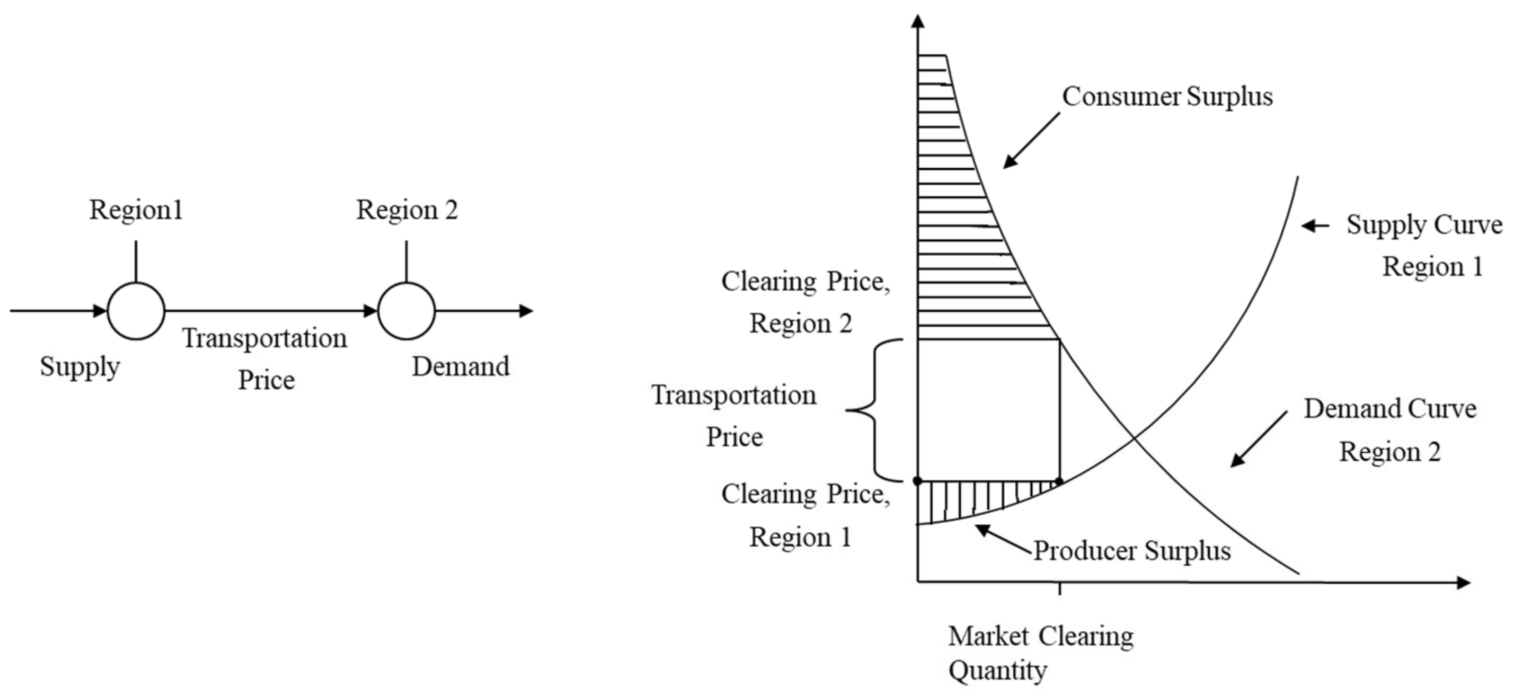
This simplistic model assumes that one can determine the functional form of the supply and demand curves relative to price in each local market. In most markets, however, either the supply or the demand is only indirectly known because it is a composite of several potential suppliers spatially separated from the market for consumption (or several potential customers spatially separated from the market for production). In the natural gas market, the supply of natural gas can be consumed by a local market, but there are options for the supply to travel through transportation pipelines and LNG cargos to be “exported” from one market into another.

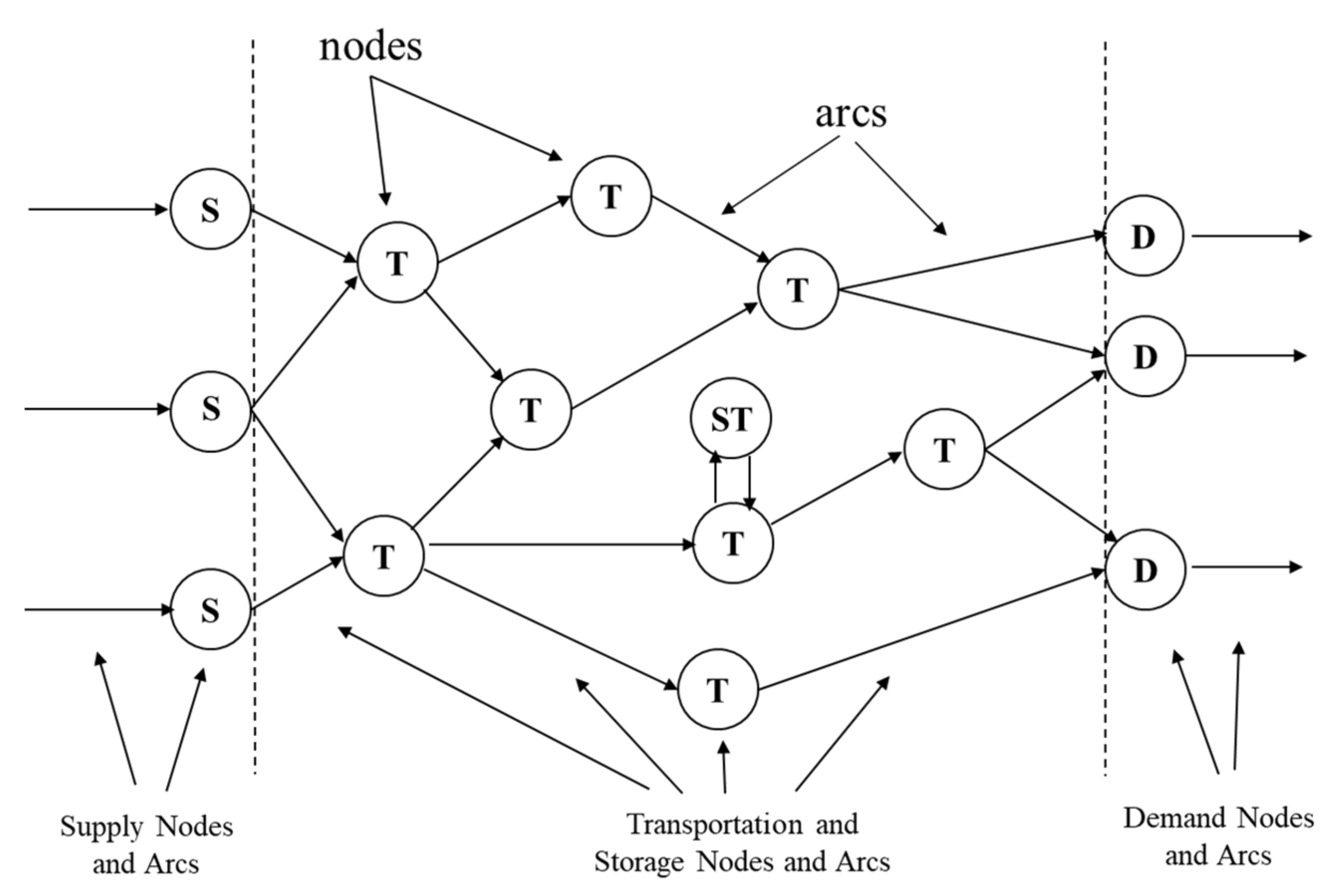
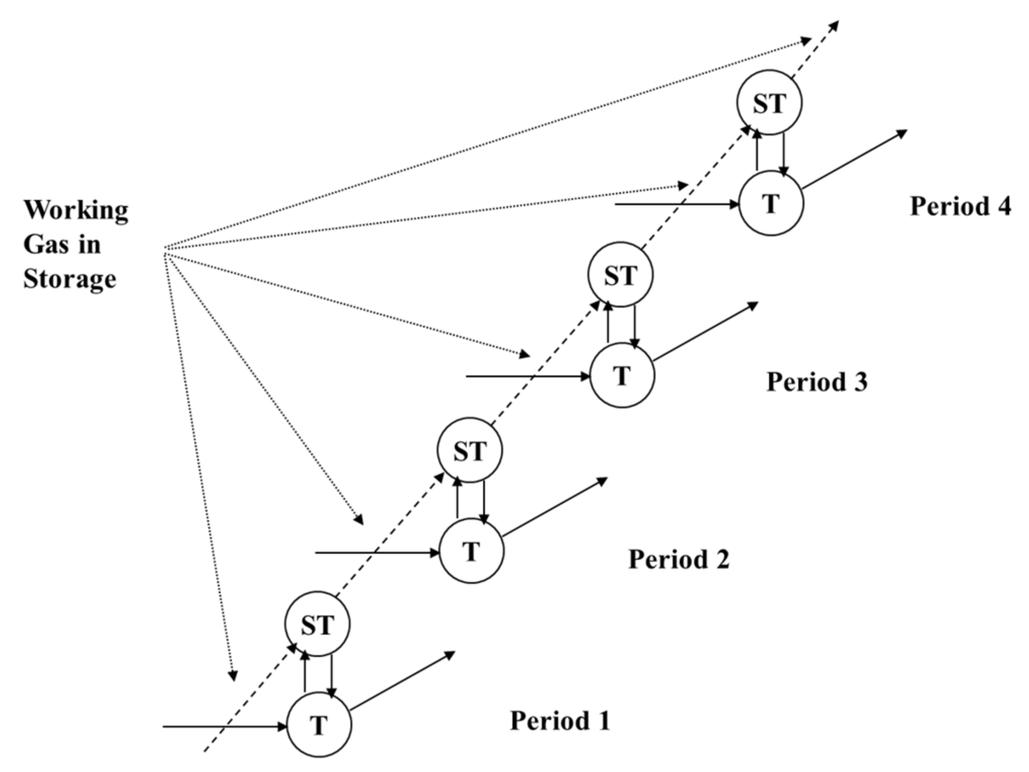
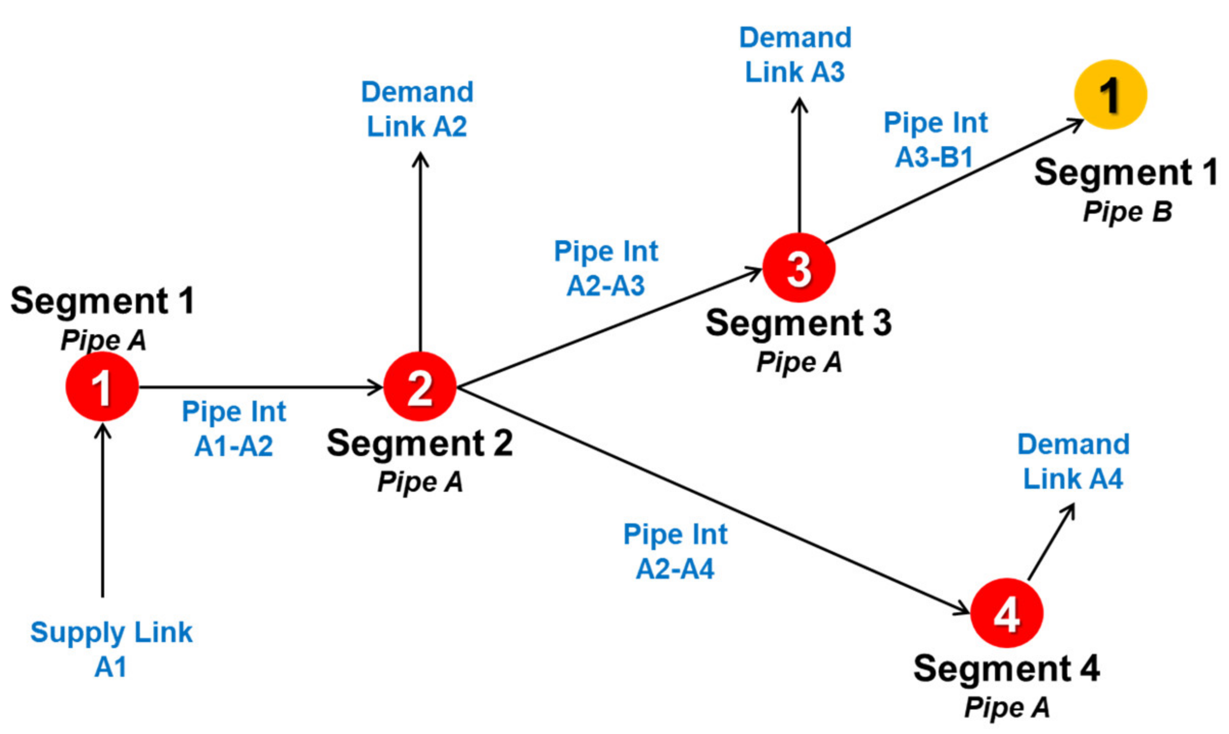
G2M2^® is designed as a network model, which is possibly the most important of the special structures in linear programming. Figure 1 presents a common scenario of a network-flow problem arising in industrial logistics concerns the distribution of a single homogeneous product from the supply (origins) to demand, such as consumer markets (destinations). The product need not be sent directly from source to destination but may be routed through intermediary points with further capacity restrictions that limit some of the transportation links. The objective is to minimize the variable cost of producing and shipping the products to meet consumer demand. The sources, destinations, and intermediate points are collectively called nodes of the network, and the transportation links connecting nodes are termed arcs. In reality, the model often represents a continuous market through time, with storage being one important infrastructure feature that can link a node from one period to the next, This is essentially the same idea as a network, except in a different dimension, as in Figure 2 Natural gas underground storage is modeled as a link between periods of the network model in G2M2^®.

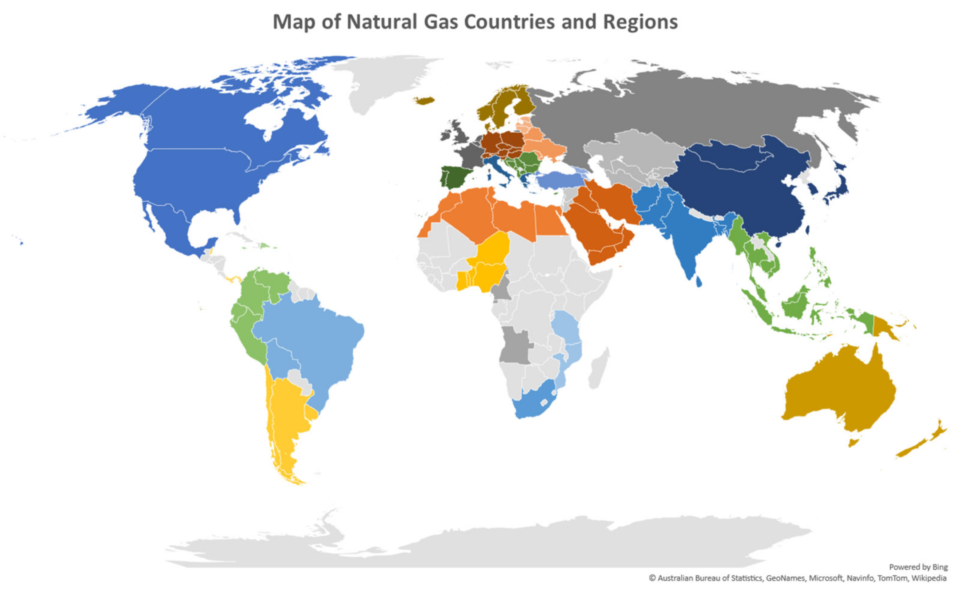
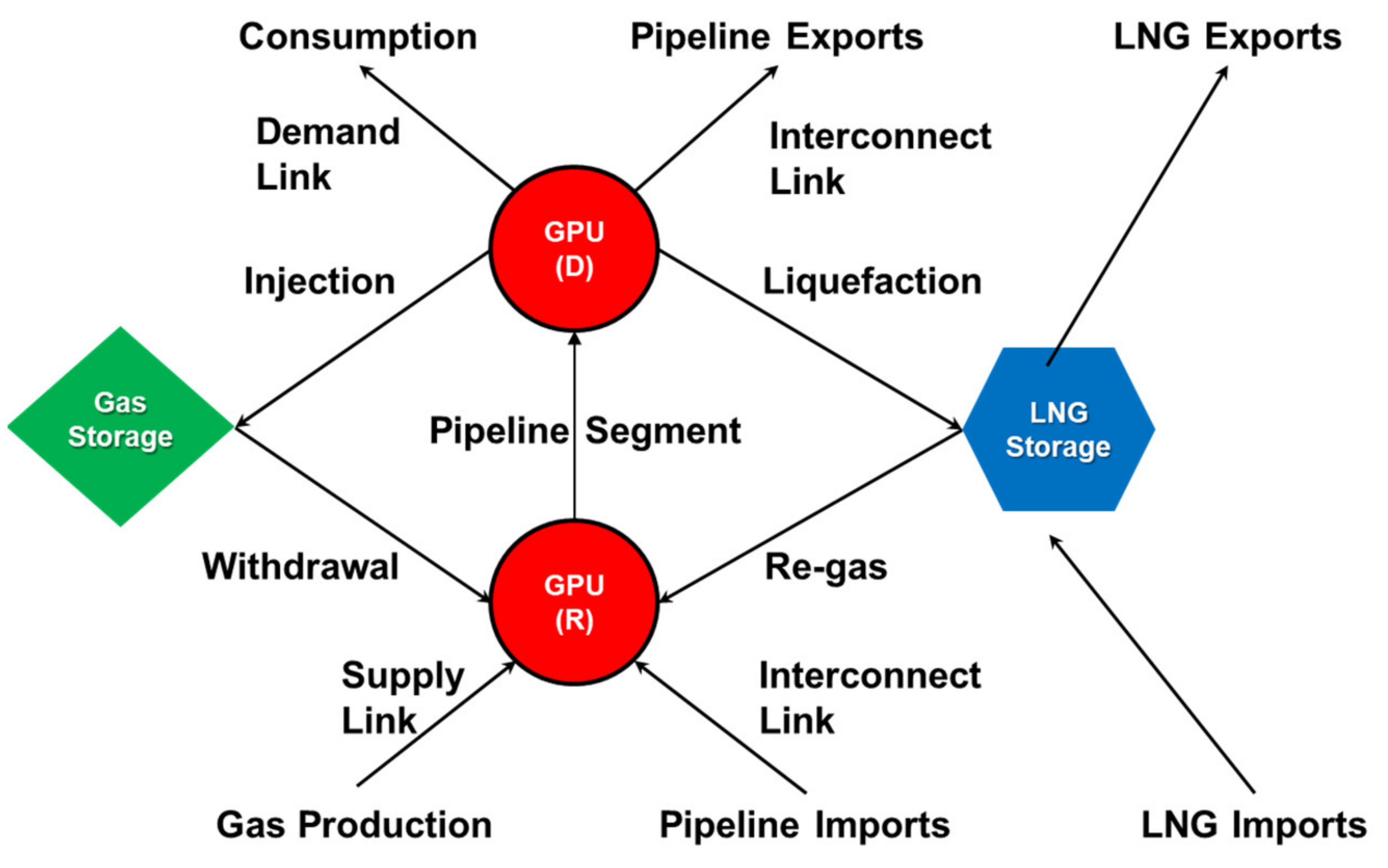
In G2M2^®, it covers all the countries that produces and consumes nautral gas in the world, in Figure 3. The most basic unit of the market is called a GPU, or geopolitical unit. In most cases, these are equivalent to a country, whereas for some large countries, such as China, Russia, and Australia, there can be multiple GPUs. For the full list of definition, see Appendix A. Each GPU as a locally defined market has its necessary components of a market, if that applies. Unlike the classic example of a network model in each GPU there are a complete set of definitions of a market node, including the options of having local demand, local supply, and infrastructure (pipeline, storage, and LNG)shown in Figure 4.

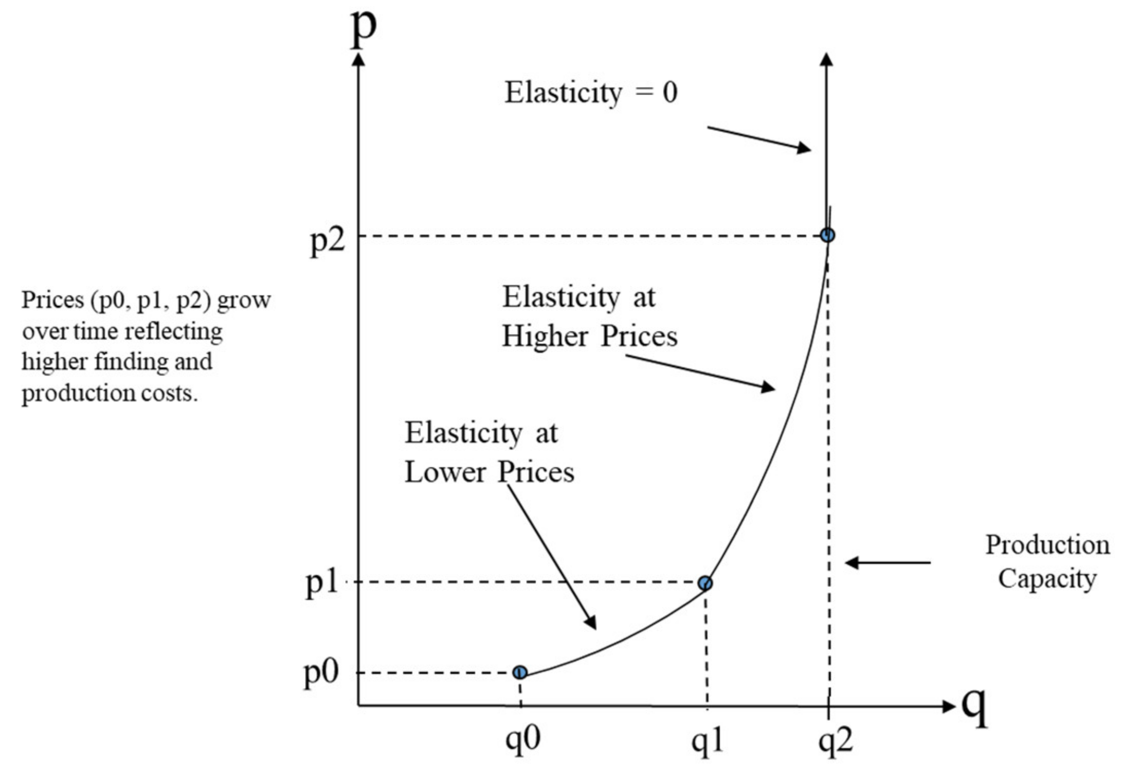
In the classic textbook version, the total number of units produced at each supply node and the total number of units delivered at each demand node are assumed to be known. In G2M2^®, the local supply and demand are described as functions of prices. For function, it is defined as a multisegment curve. This is because there are operational limits in how supply can respond to price changes. While supply responds nonnegatively to price increases, when it becomes closer to the production capacity limit for a given period, supply elasticity of price decreases. This is an important and practical assumption; although there is some flexibility of operation, the supply response in natural gas follows a production plan that leads to lagged supply responses, and a short-term capacity limit exists.

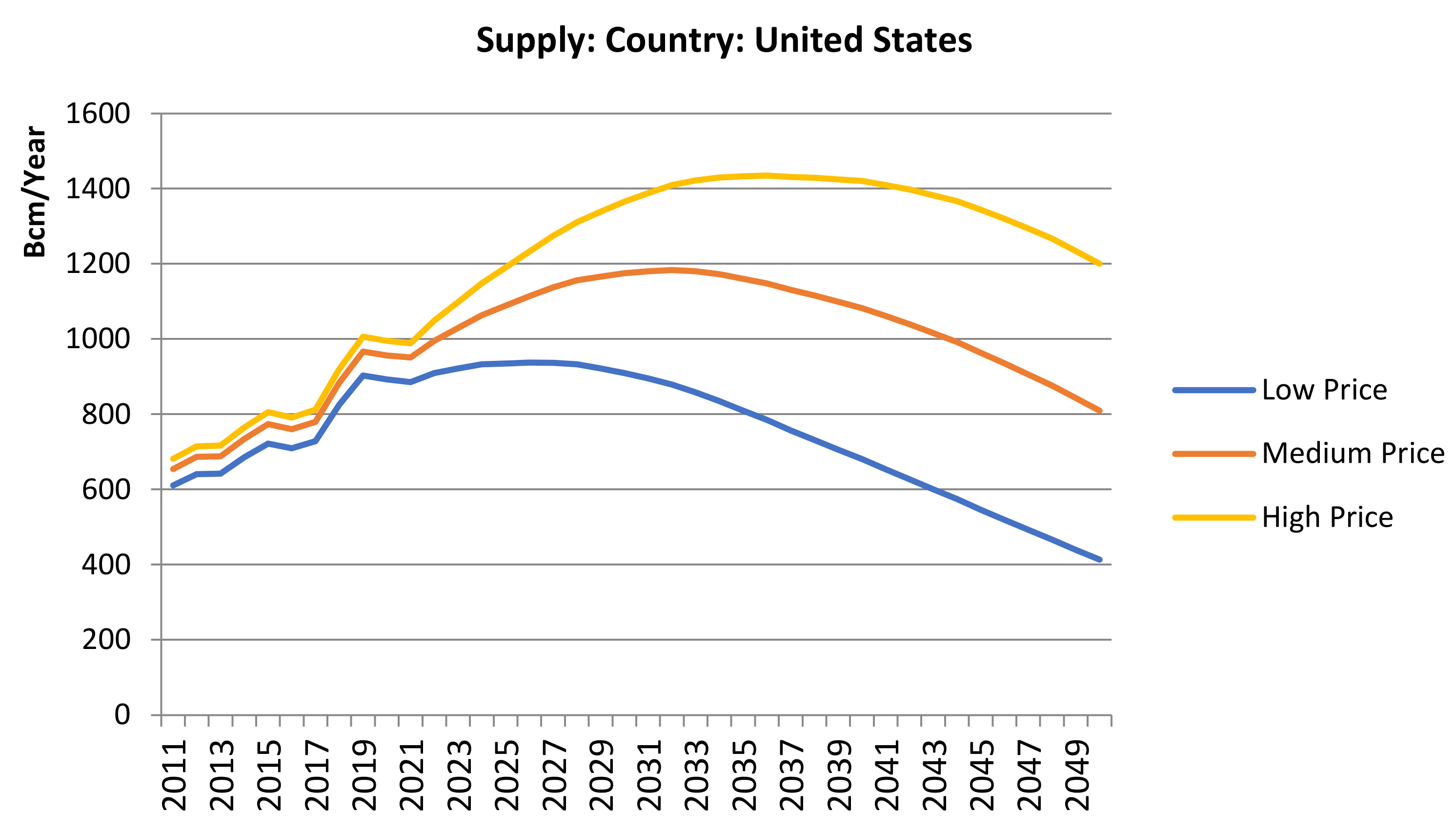
There is a supply curve for each period that crosses different prices, such as what is shown in Figure 5, where only quantity and prices are graphed but not time. If one takes the family of supply curves across a time period and then graphs the supply quantity along the curves at a given price path, we are given supply curves over time at a given price scenario. This is shown in Figure 6 in three price scenarios: low, medium, and high. Here, when limited to a two-dimensional graph, one can only see time and quantity.

In G2M2^®, the demand curve is determined by gas prices as well as additional factors, including GDP, the population, and weather conditions. Graphically, it can be described as a multisegmented, downward-sloping curve. The rationale for the different elasticity of demand comes from the cost of switching and the availability of an alternative to gas in different downstream applications. Five segments of demand are modeled here: residential, commercial, industrial, power generation, and transportation (here, transportation implies the natural gas demand for the transportation sector, for any vehicles or vessels that use natural gas as a transportation fuel). Each has distinct assumptions and function definitions based on different driving factors.

$$D=C\times P^{-e_p}\times H^{-e_h}\times M^{-e_m}$$

where:

• D: Demand Consumption;
• C: Constant;
• P: Gas Price;
• H: HDD (Heating Degree Days);
• M: Macro Variables such as customer counts, GDP, manufacturing GSP (Gross State Product);
• e_p: Gas Price Elasticity;
• e_h: Weather (HDD) Elasticity;
• e_m: Macroeconomic Elasticity.

With separate supply and demand functions defined for a local node, G2M2^® connects them to a model of the actual infrastructure grid, which is made up of pipeline, LNG, and underground storage. They provide options to transfer and reallocate a commodity from one market to another, as long as the market price can incentivize such a transaction across markets. Figure 7 shows a market clearing, including the options for transportation across a region. Figure 8 and Figure 9 show the setup of pipeline transportation and LNG in G2M2^®.

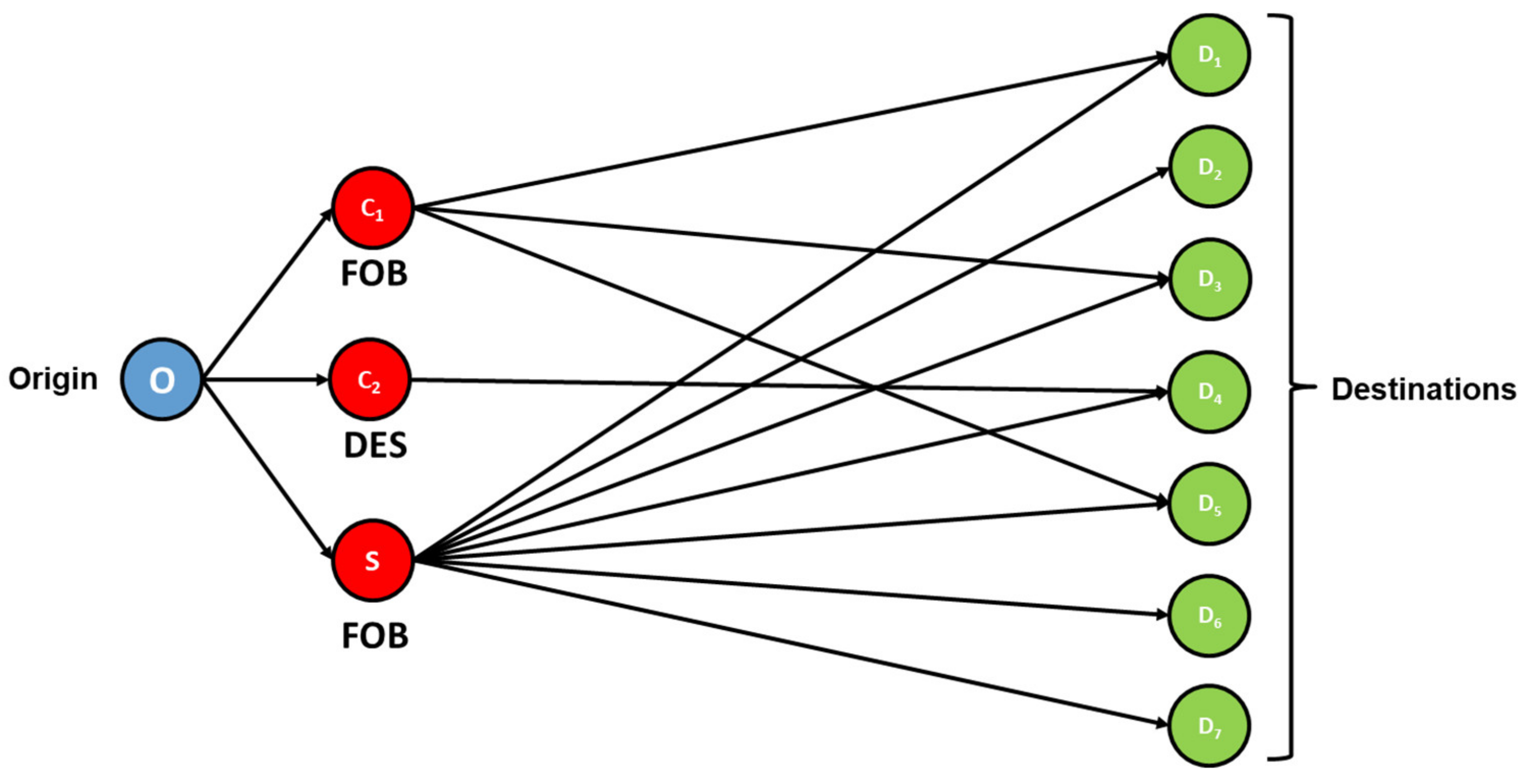
LNG is an alternative transportation option to a pipeline for natural gas, but it has more flexibility in options compared to a pipeline. Buyers and sellers of LNG cargos across the world can trade without the physical constraints of a fixed route such as a pipeline. However, there are existing LNG contracts that help to bring additional constraints to LNG trades to some extent in order to reflect the needs of risk management and securing supply/demand in the market. In G2M2^®, LNG contracts are modeled explicitly with options to limit destinations and origins per contracted terms, in addition to spot trading, which represents a transaction determined only by market price and the balance at a given period.

This trading behavior of the natural gas market is complex for several reasons:

First, there is an increasing number of players in the markets, including both producers and consumers in the global natural gas market. Second, there are various transportation limits. Each infrastructure option—pipeline, LNG terminals and tankers, and underground storage—has its own capacity and operation limits. This describes the transportation limits and optionality of a market. Transportation connectivity is often the cause of price spikes in the market, especially during extreme weather. Third, in addition to the infrastructure limits, there are additional constraints such as contracts and LNG tanker cost and availability, pipeline tariffs, and transportation contracts for pipeline gas and LNG.

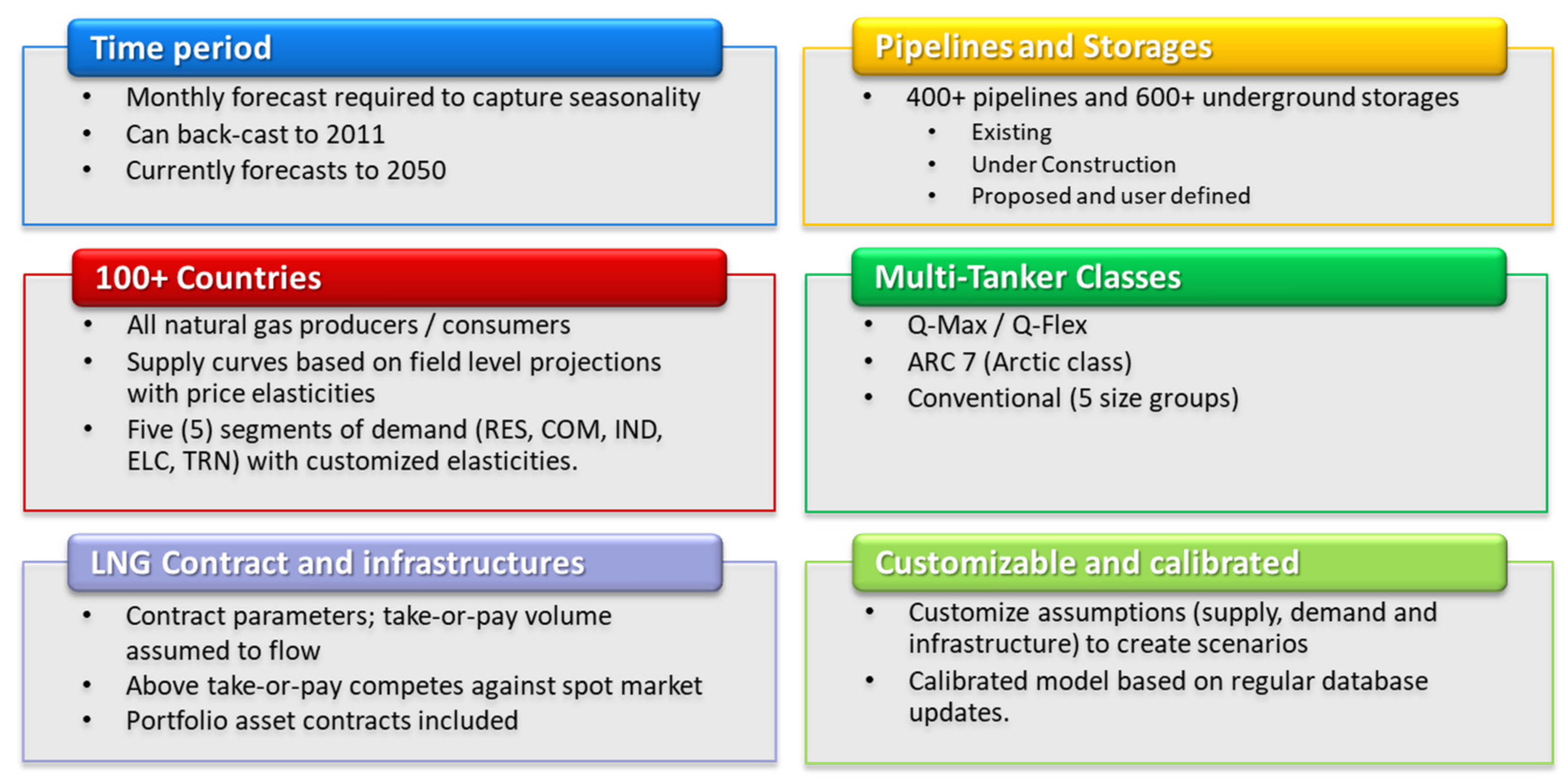
One advantage of the G2M2^® model is its focus on representing the actual pipeline systems and infrastructure terminals covering the global market. It models pipelines, liquefaction terminals, regasification terminals, and underground storage in almost all gas-consuming and gas-producing countries. Even though this results in a much larger model than using a corridor or nodal approach, it offers much greater analytical power. One can make projections about specific pipelines and numerous pipeline-specific market points, as well as rolling up flows and averaging prices over higher-level geographical areas. Such a model also allows one to take pipeline company information from government and industry sources and to apply that information directly without having to perform a lot of manipulation and approximation to make it fit an unnecessarily aggregated corridor or nodal approach. Without going into much detail, here is an overview of what is covered in a G2M2^® database.

4. Model Validation

As described above, G2M2^® is a complex network model involving hundreds of supply and demand areas connected by both pipeline grids and LNG tanker pathways. It is further complicated by the fact that gas can be stored underground for long periods of time in order to provide supplies when needed during periods when it is most needed (usually during cold winter months). Each of these components of the model (supply, demand, and infrastructure) requires detailed information that reflects what actually occurs in the global natural gas market. Data researchers at RBAC, the developer of the G2M2^® simulation system, have spent decades of person-years collecting, organizing, and testing the data needed by this and similar gas market simulators in a structured and meaningful way summarized in Figure 10. The selections they have made have been proven to provide consistent results that match actuals to a reasonable degree when G2M2^® is executed over historical time periods.

RBAC releases an updated database about once a quarter. Here are a number of the primary data sources for the G2M2^® base case database in

Table 1. Primary data sources for G2M2^® base case database.

Data Source	Usage
Rystad Energy’s UCube Database	Gas production (historical and outlooks)
Joint Organizations Data Initiative	Gas production, storage, consumption, imports, exports
UN Energy Database	Gas production, consumption by end use, as fuel, etc.
BP	Gas production and consumption; LNG and pipeline trade
ENTSOG	Gas pipelines in Europe; development plans
GIIGNL	LNG import and export terminals, tankers, contracts
U.S. EIA	Detailed gas market data for the U.S.
EEX	Gas prices at European virtual trading hubs

:

Because there is no undisputed “best source” for all of this information, G2M2^® identifies historical data points for supply, demand, storage and trade volumes, via extensive cross-comparisons of data reported by the various sources. For example, BP’s Statistical Review of World Energy is a well-respected source of information on natural gas as well as other energies. It has a long history of reporting annual gas production and consumption at the country level for major producers and consumers. It reports similar information on LNG production and trade. The United Nations database contains much greater detail for each country and year, including the source of gas, sector of use, use as pipeline or other fuel, etc. It is also compiled by year by country. However, it is not as current as BP. Finally, JODI provides country-level information on production, consumption (total and to make electricity), storage, and LNG by month-of-year back to 2009. Since G2M2^® uses a monthly periodicity, this information is very valuable. It shows seasonality that both the BP and the UN data miss.

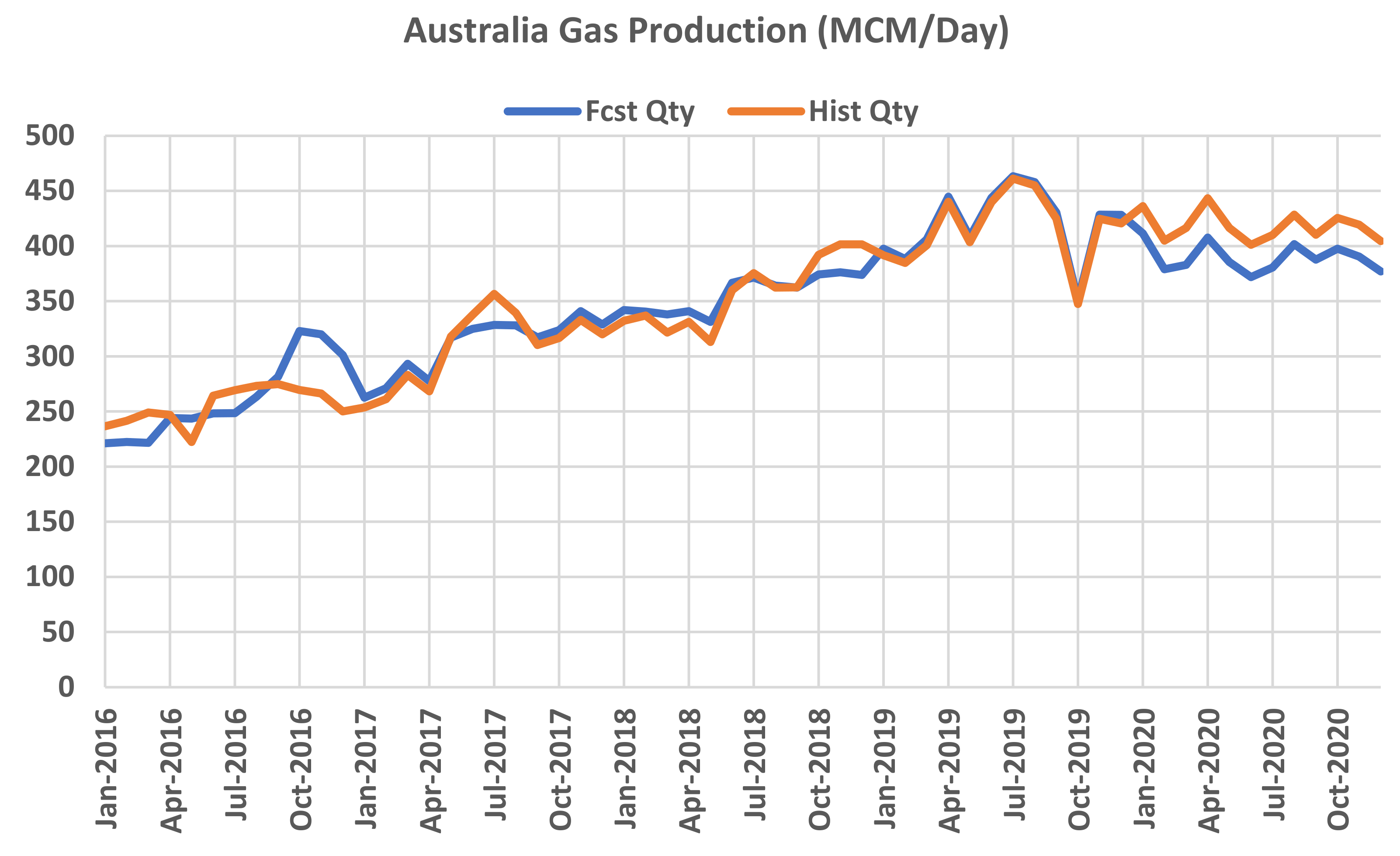
RBAC validates each base case release by setting the specific values for historical monthly supply targets (along supply curve), demand targets (along demand curve by sector); storage levels; pipelines (capacities, fuel use, and transportation cost estimates); LNG export and import terminal capacities; and fuel use, cost, and contracts.

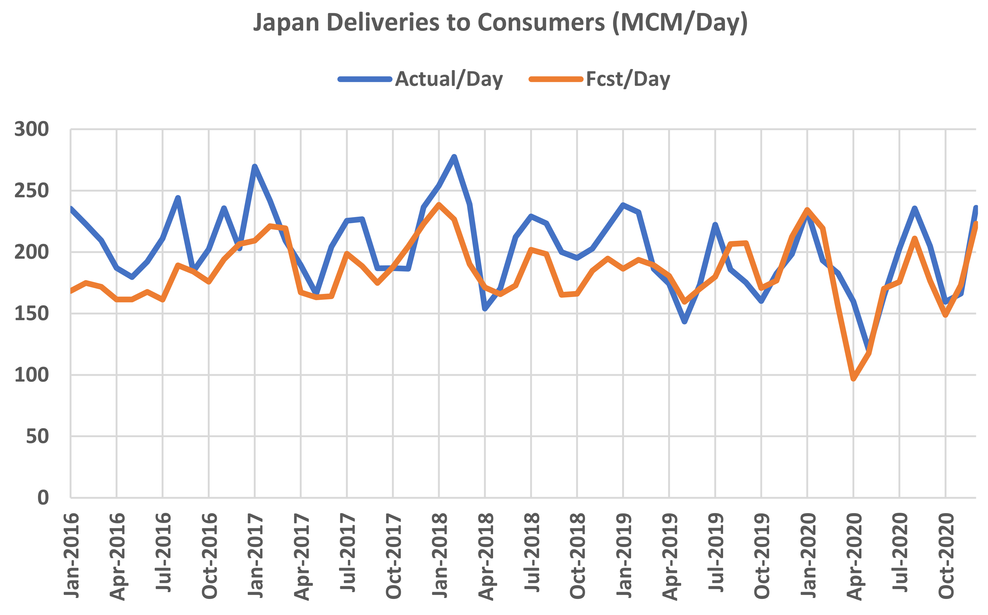
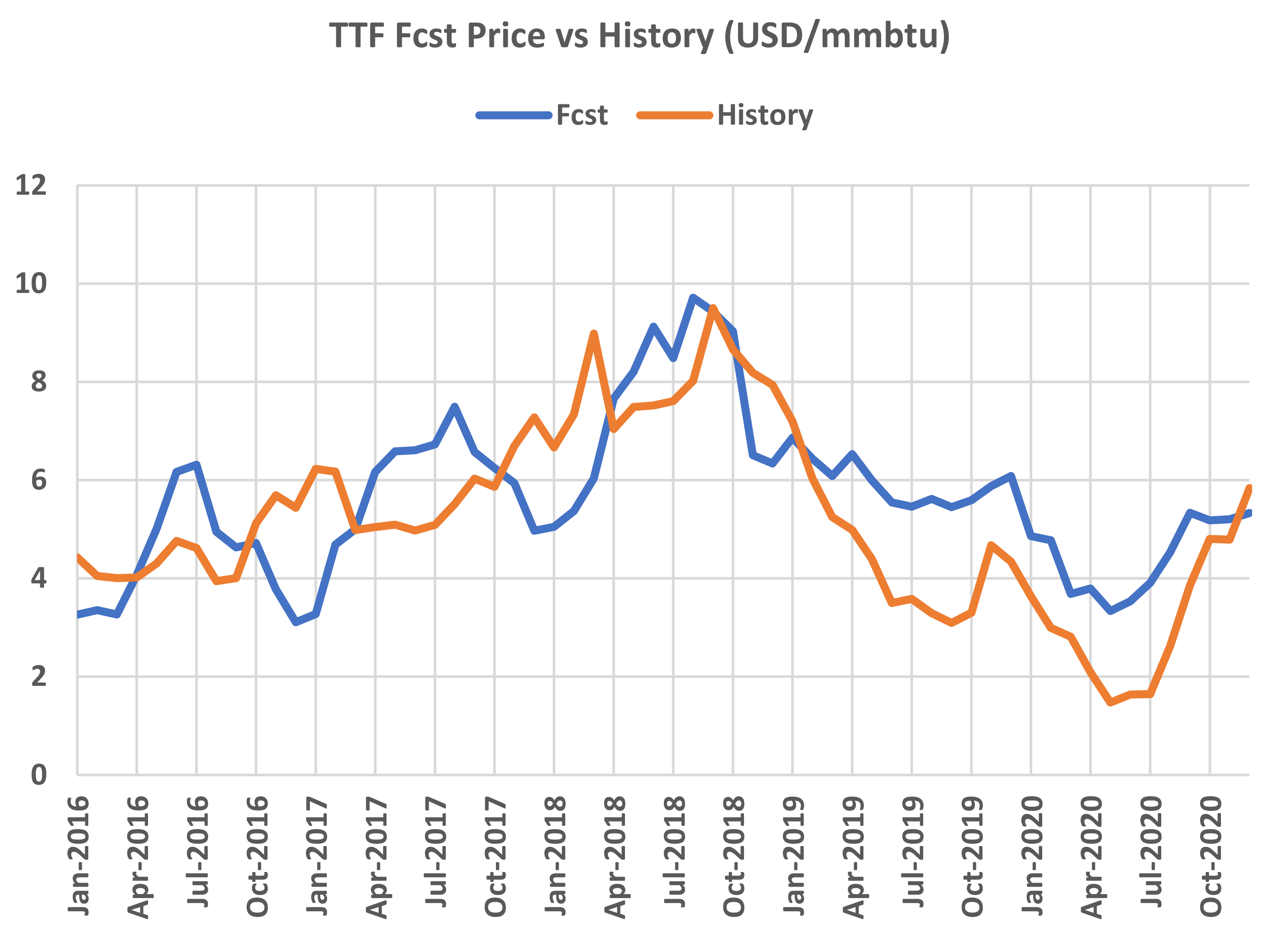
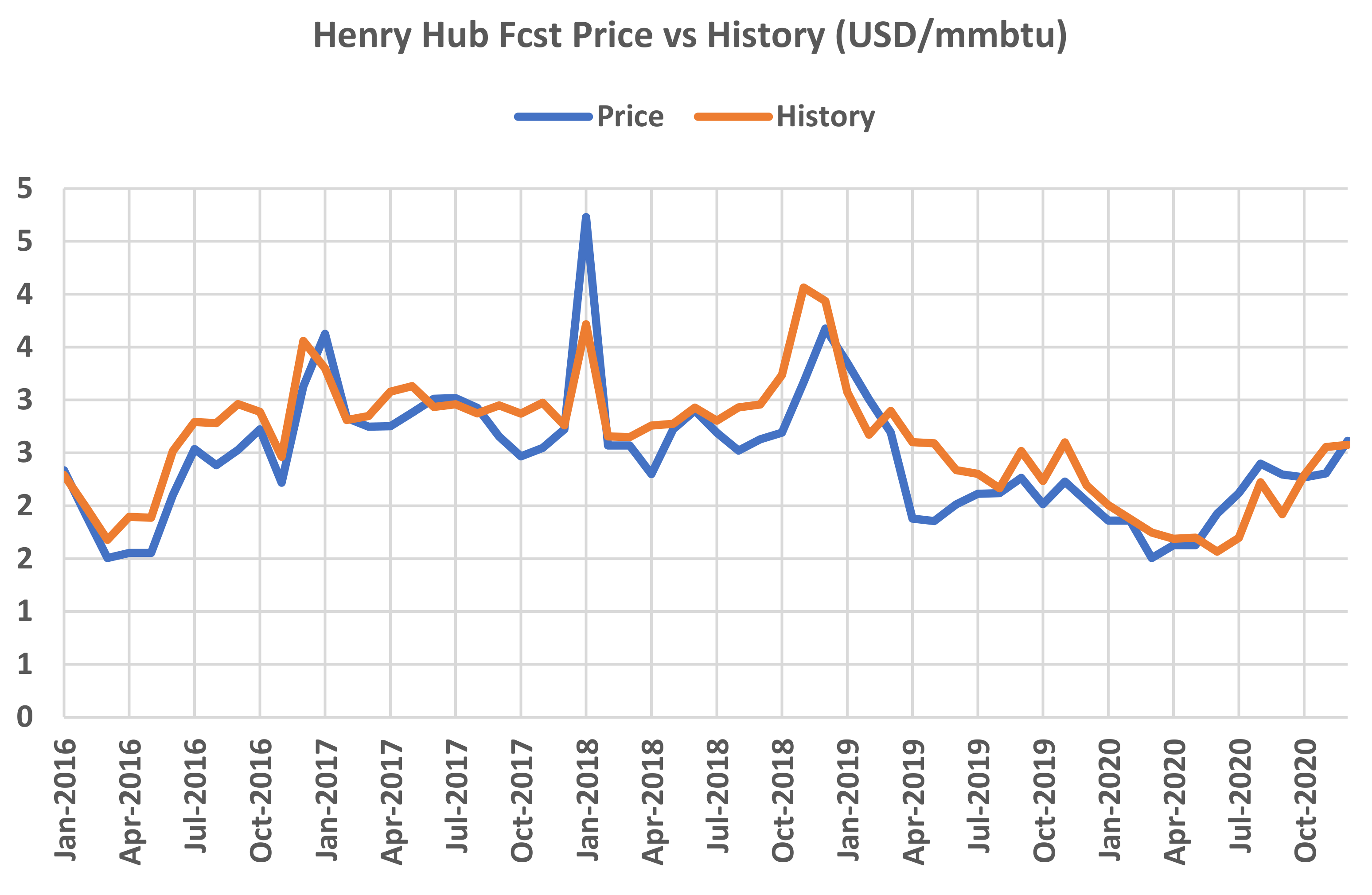
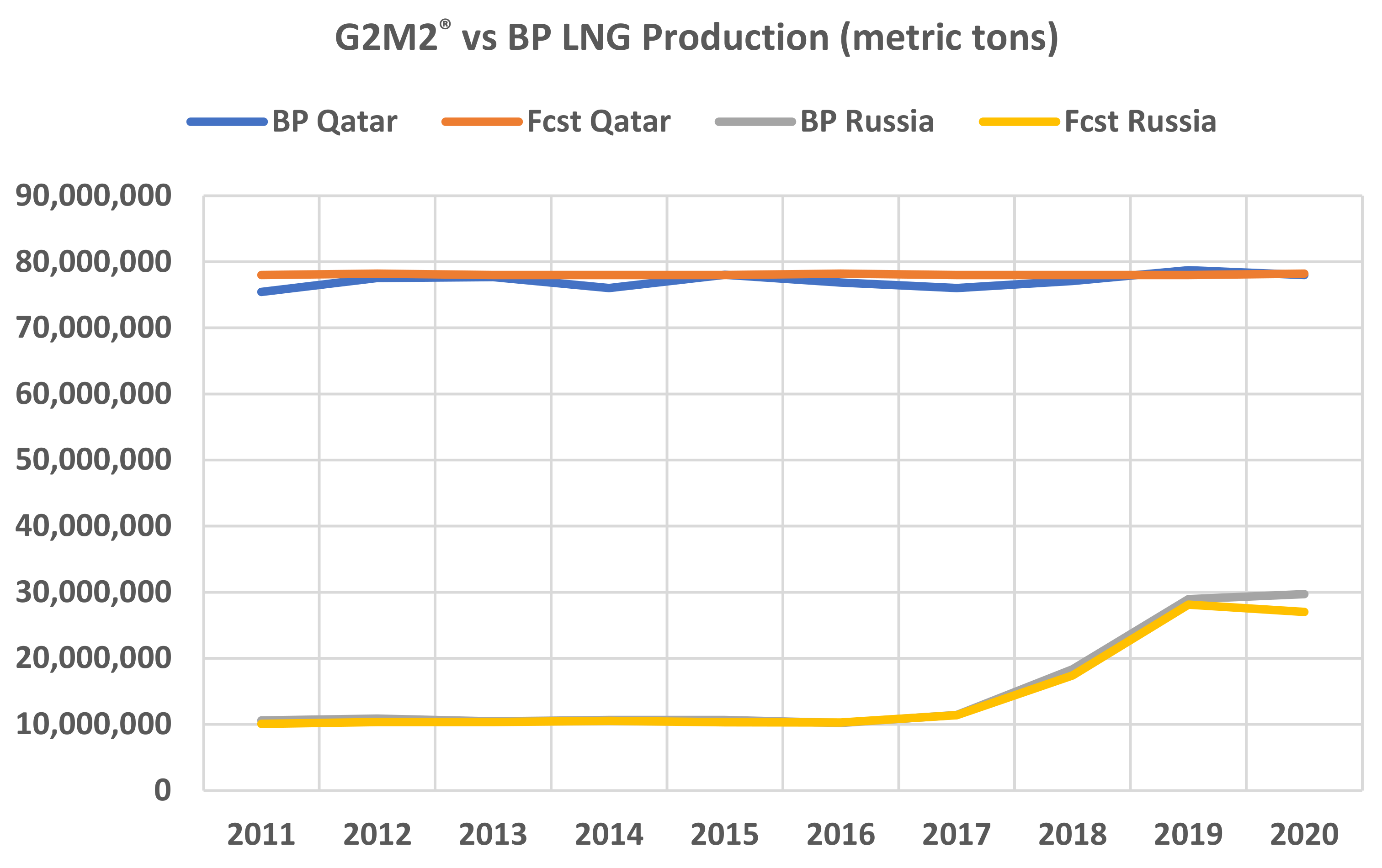
It then makes validation runs over the historical period from 2016 to 2021 to determine if it fits historical data to a reasonable degree by mathing the forecast to historical values or quantities including historical gas production, consumption, and storage; LNG production and exports; and market prices. Figure 11, Figure 12, Figure 13 and Figure 14 are some examples from a recent set of validation runs for supply, demand, and prices.

Validation is a continuous process. There are a huge number of potential comparison points. Many will provide good matches, but some will not. The challenge for the G2M2^® development team is to continue to identify areas where improvements can be made and then determine the right course of action to make those improvements.

5. Global Gas Market Overview

The objective of this paper is to use G2M2^® to model potential impacts on the LNG trade under different long-term scenarios of gas markets under an energy transition. Instead of using one scenario, this paper provides two scenarios to compare and extract findings. The difference between the two scenarios drives value. In order to set the stage for the comparison, this section is organized in the following way. First, we share long-term assumptions and outlooks that provide an understanding of the natural gas and LNG market going forward. Second, we discuss the key assumptions that would be impacted using an alternative low-carbon scenario. Since it is not clear what overall energy transition policies there would be across nations, this paper addresses one of many possibilities as an example to illustrate how scenario planning could help answer this question. The intent here is not to cover all possibilities but to demonstrate how a structural economic model helps to describe a significant shift in the market. Lastly, we discuss the results and differences between the alternative scenario versus the base case scenario.

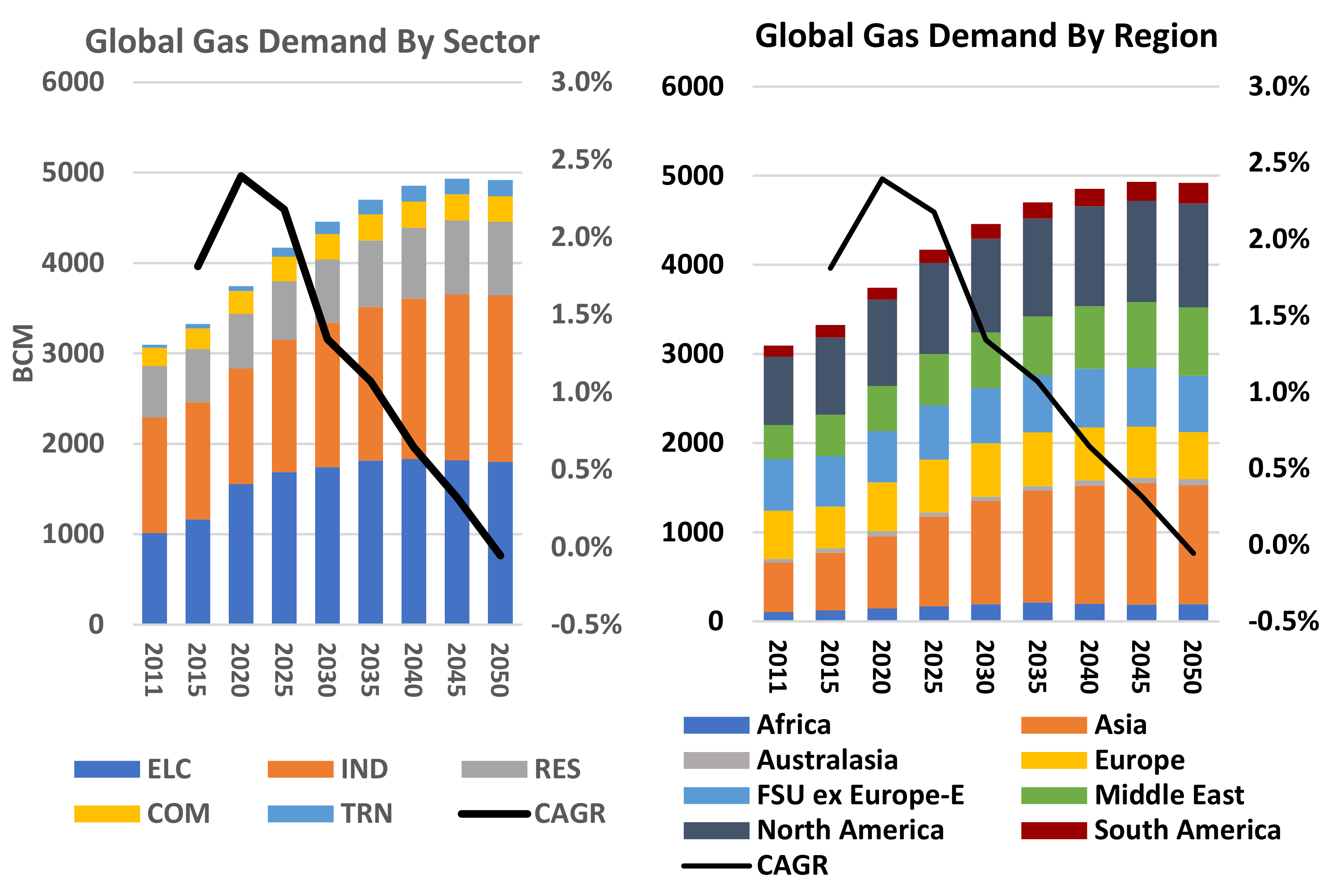
Figure 15 shows the global gas demand forecast through 2050, by sector and by region. The global gas market experienced fast growth during the five years from 2015 to 2020, at around 2.4% compound annual growth rate (CAGR) despite COVID. We estimate that global gas demand, which comprises five sectors, Residential (RES), Commercial (COM), Industrial (IND), Electricity Generation (ELC), and Transportation (TRN), will continue to grow above 2% for the next five years. Currently, our global gas demand is around 4000 billion cubic meters (BCM) in total, seen here with only the final consumption by sector. Therefore, it looks to be about 3800 BCM (with about a 5% loss in transportation and processing of gas).

Based on the G2M2^® base case scenario, there is 1600 BCM (which is around 42 TCF) incremental gas demand by 2050, of which two-thirds of the growth would occur during the next decade. If we break down the demand outlook by major regions and by sector, we should have a better understanding of the key drivers:

○

By region, Asia, the Middle East, and North America are the top markets in terms of volume, followed by some steady growth in South America.

○

Africa has great potential in the long term. However, at this point, its lack of infrastructure will be a major roadblock for scaling up its electricity generation of fossil fuel to meet a fast-growing population.

○

By sector, it is clear to see that the drivers would be electricity generation and industry demand.

There is a gradual slowdown of gas growth, especially in developed countries, implying that the global gas demand peaks somewhere between 2040 and 2050. This would be driven by global climate policies. In the base case scenario, there are no clear net-zero policies implemented in countries; instead, there are a set of country-level policies being adapted to describe changes in natural gas demand, especially for the power-generation sector.

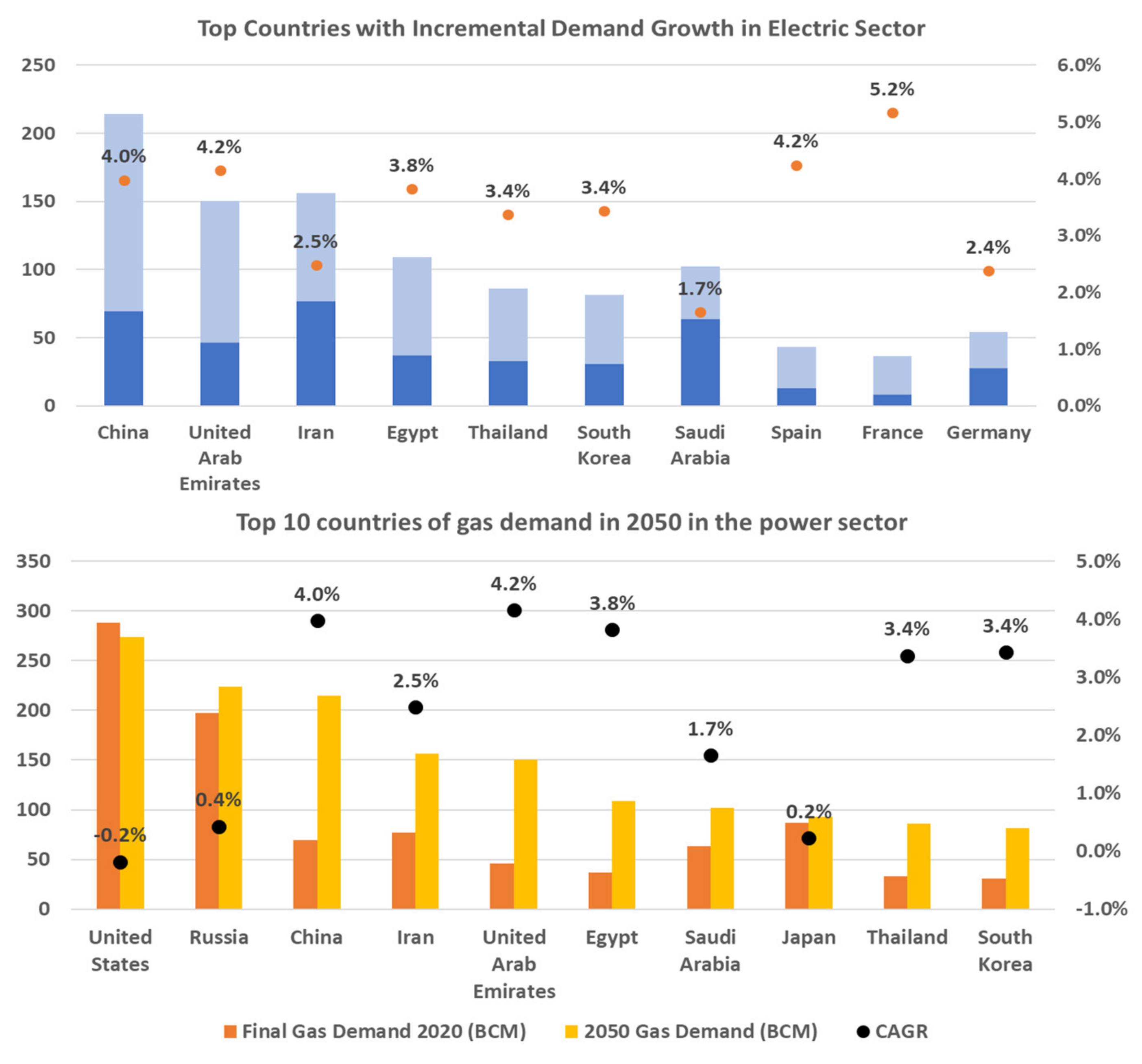
In the G2M2^® model, there is a separate electric demand model that explicitly models the key drivers from generation mix to climate policy as a function of the natural gas demand for the power generation sector. The upper graph in Figure 16 shows the top countries with the greatest incremental demand growth in the electric sector for the next three decades. The dark blue part is the current gas demand for power generation, whereas the incremental volume is in light blue. The compounded growth rate is calculated and plotted for each country on the secondary axis. This graph provides additional information from the previous graphs on regional growth: out of 10 countries, there are only three from Europe, three from the Middle East, one from North Africa, and three from Asia. The graph below shows the top 10 countries with the greatest total gas demand for power generation in the world by 2050. The orange bar is the 2020 level, and the yellow bar is 2050. We can see that 7 out of 10 countries from the second graph also happen to be ones from the first graph and have the highest incremental growth. The U.S./Russia/Japan are the top countries in terms of power growth but are quickly being caught up to by emerging markets.

Furthermore, a set of emissions targets and generation shares are considered in the current base case, shown in

Table 2. By country, energy transition goals and market and generation share targets (the country-level climate targets are updated regularly based on IEA/IRENA Renewables Policies Database).

Country	End Year	Target Fuel	End Year Target
Switzerland	2031	Nuclear	0%
South Korea	2040	Renewable	35%
Belgium	2025	Nuclear	0%
Germany	2022	Nuclear	0%
Germany	2040	Coal	0%
Japan	2030	Oil	0%
Mexico	2024	Renewable	35%
Vietnam	2030	Renewable	10%
India	2030	Renewable	40%
Netherlands	2023	Renewable	16%
Denmark	2050	Coal	0%
Denmark	2050	Oil	0%
Denmark	2050	Natural gas	0%
Uzbekistan	2025	Renewable	20%
Algeria	2030	Renewable	27%
Australia	2020	Renewable	24%
Libya	2025	Renewable	10%

.

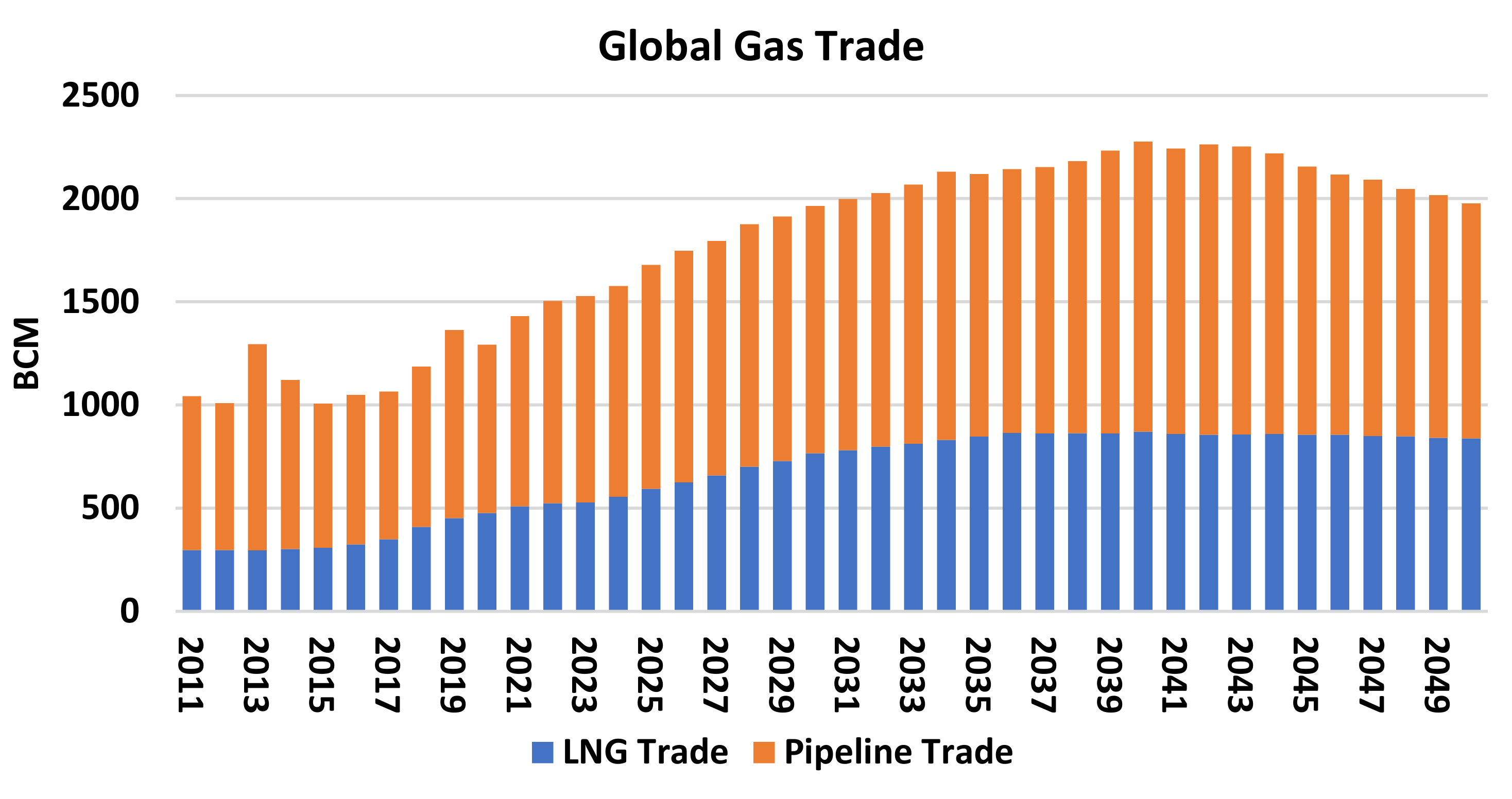
With the rising needs for nautral gas from many more countries, there is a greater needs for natural gas trade, especially LNG in recent year. Figure 17 shows the global gas trade since 2011 has been growing steadly with continuous momentum through 2040. LNG as a more flexible option of transportation is outgrowing the needs for pipeline trade. There are many LNG projects going up around the world. 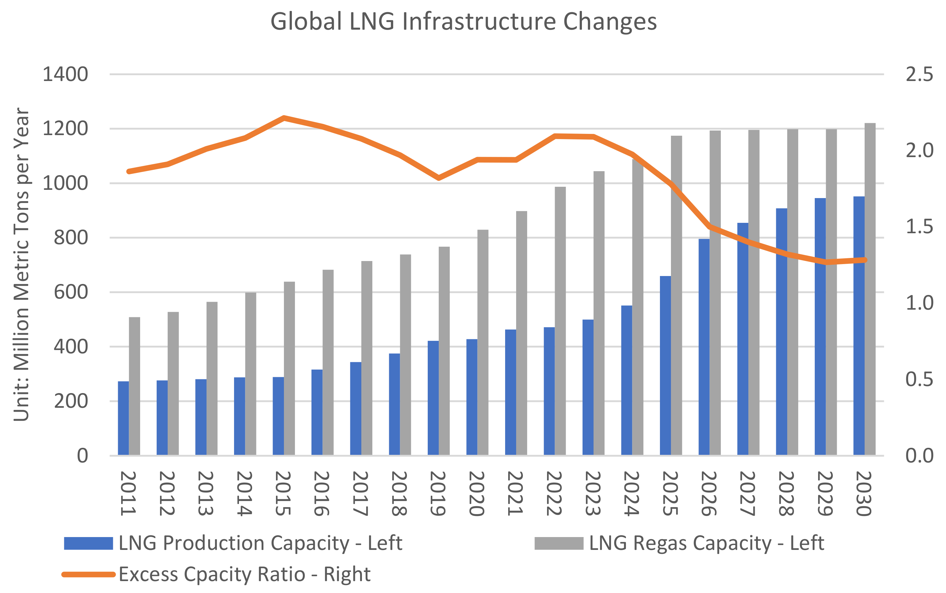Figure 18 is a graph of global LNG production capacity versus regasification (regas) capacity, and the orange line shows the ratio of regas/liquefaction. In the past 10 years, as more liquefaction facilities have come online, the orange line has started to decline. As the regas projects continue to come online in Asia, the orange line is pushed up starting around 2020–2023, while some delays in liquefaction will cause ramping up around 2023–2025, bringing excess capacities online. In G2M2^®, besides the existing LNG terminals, all projects that are under construction or after FID are also included starting at a future date. There are projects that are proposed, which is clear from the online date, which are excluded from the database at the moment.

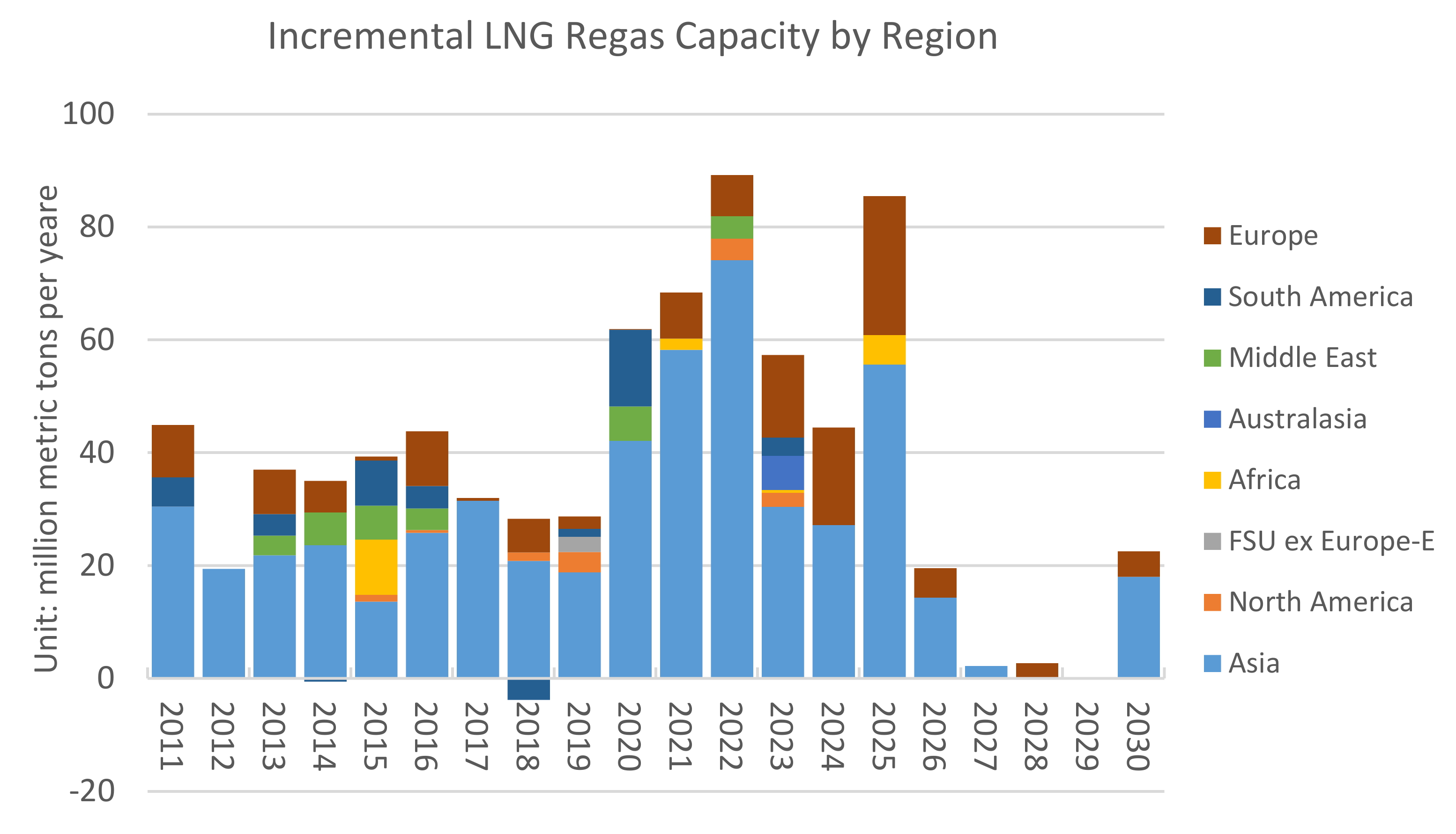
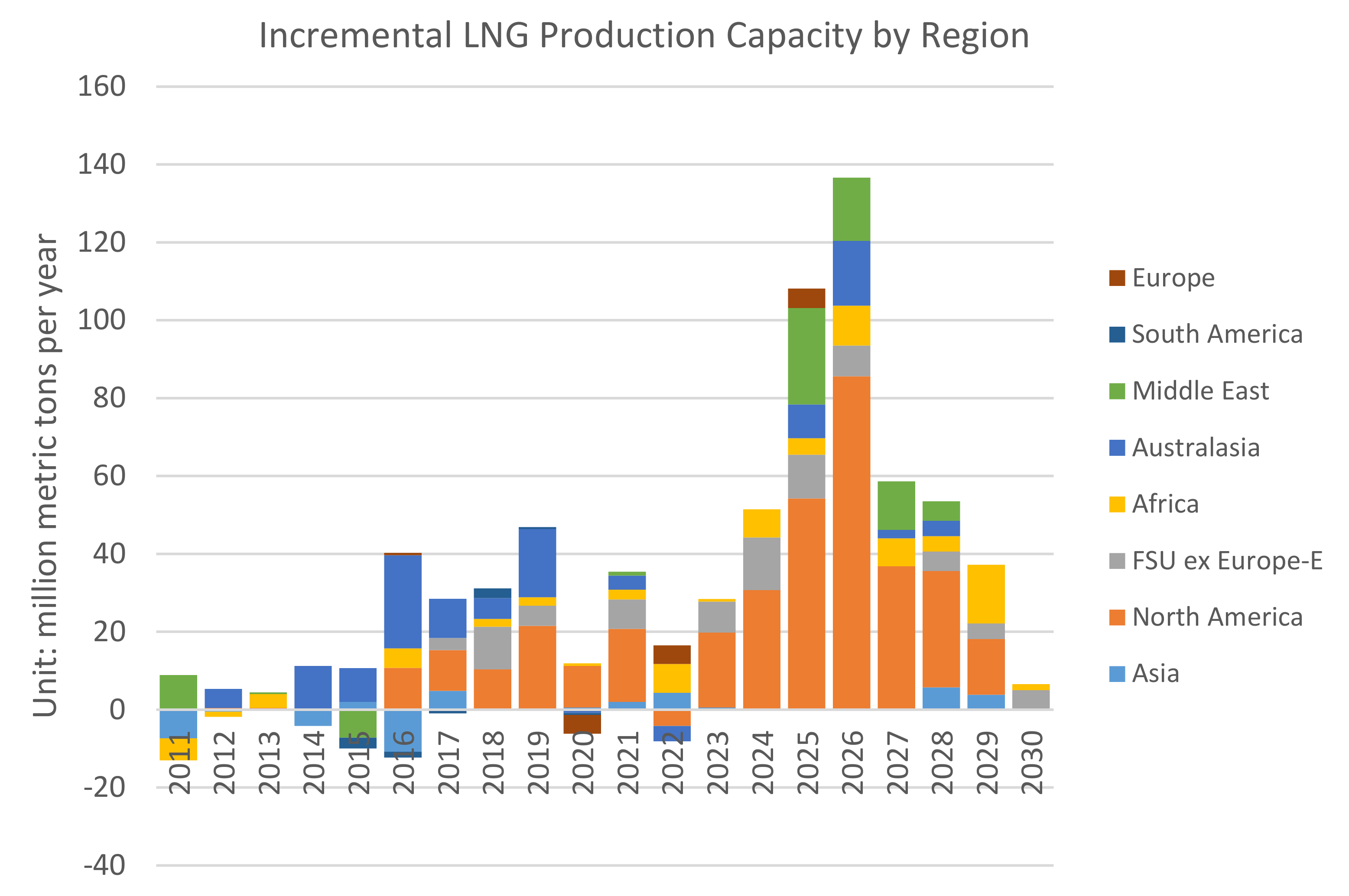
Figure 19 and Figure 20 present incremental LNG capacity by region for both production and regasification. The major expansion of LNG regasification is in Asia: for 2020–2023, an incremental 260 million tons in capacity (~3.3 bcfd). A major expansion of LNG liquefaction is going to be in North America, followed by Russia, the Middle East, and Africa: for 2024–2026, an incremental 330 million tons in capacity (4.3 bcfd). For 2020–2030: while 225 million tons of LNG (11 tcf) are expiring, there are 140 million tons (6.7 tcf) of contracts being currently added. In 2020, about 1 tcf of new contracts will be starting. Going forward, portfolio contracts with flexible destinations will take 60% of the incremental volume.

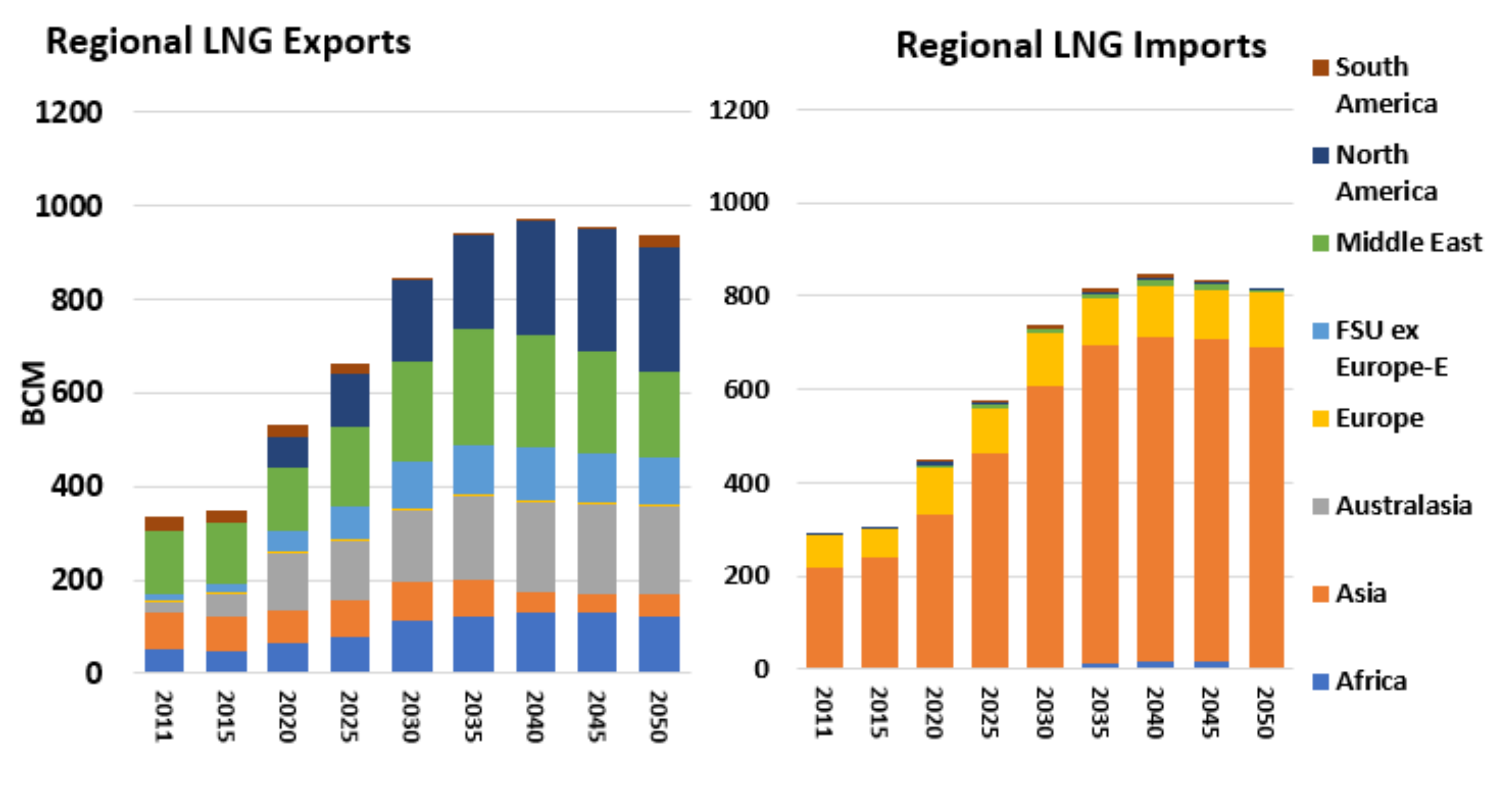
For the current LNG market, although we are modeling a competitive equilibrium, it is important to note that there are certain markets and players influencing the market with its scale of demand or supply. These players will still price the market, but their decisions have more influence on equilibrium prices and quantities. Figure 21 shows the forecasted LNG export (supply) and import (demand) outlook. On the supply side of LNG, North America, Australia, and Africa are the fastest-growing suppliers, challenging the position of the Middle East and Russia. On the demand side, there are two major battlegrounds. From a geographic standpoint, one is the Asian market versus the European market. This is easy to understand, as the downstream market weather and market conditions, as well as transportation costs, set these markets apart. In addition, from the types of players, one can also categorize two types of LNG buyers: existing and mature players vs. emerging markets. The existing and mature players include Europe, South Korea, Japan, and Taiwan, while the emerging markets are represented by China, India, and other Southwest Asia/Southeast Asia countries. The difference between the LNG buyers mainly lies in the type of LNG contracts and pricing terms. Finally, there is one additional category of LNG buyer that is not represented by the local market but is a portfolio holder of multiple LNG contracts. It is not the focus of this paper to go further into the details of modeling portfolio players.

As we have set up the point of view of the global natural gas and LNG industry, we will focus on the impact of the energy transition on LNG trade through a set of scenarios, which are the reference case versus an alternative scenario of accelerated energy transition for Europe.

6. Scenario Planning of Energy Transition

To keep our focus on the LNG trade, we need a simplistic alternative, but one that is drastic enough to demonstrate changes in the LNG trade, because such a scenario is simple but yet effective in illustrating how trade and balance change. In order to focus on changes, from here on we refer to two scenarios for comparison purposes.

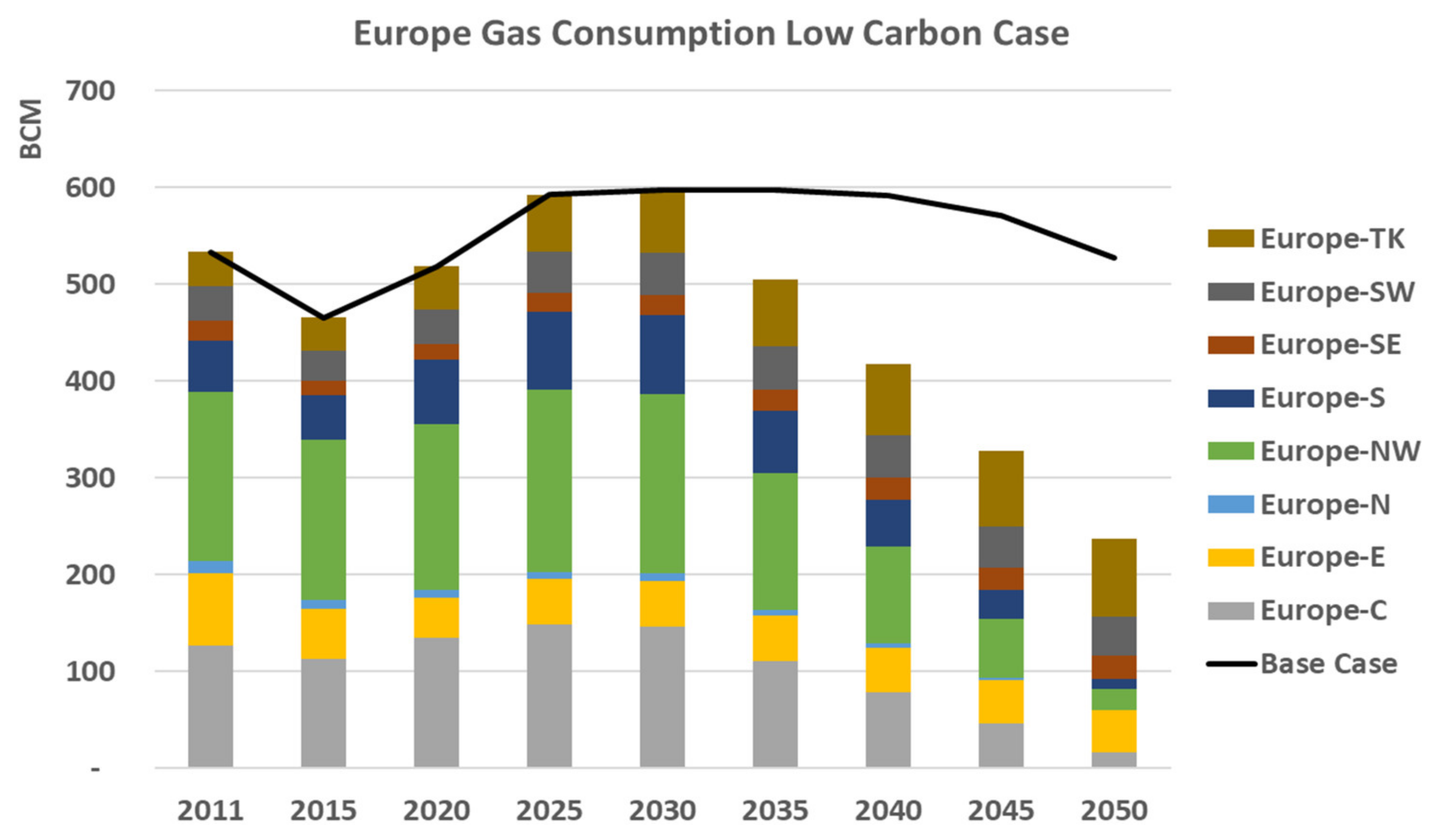
While keeping everything else constant, including any demand assumptions for the rest of the world outside Europe, as well as supply assumptions, the low-carbon case is an aggressive transition scenario for Europe, where EU countries drop to 10% of their current gas consumption level, and the whole of Europe to 45% of its consumption of its 2050. As shown in Figure 22 below, Europe consumption in 2050 is about the same level as the year 2020 for the original base case, while in the low-carbon case, the consumption drops by 55% in 2050.

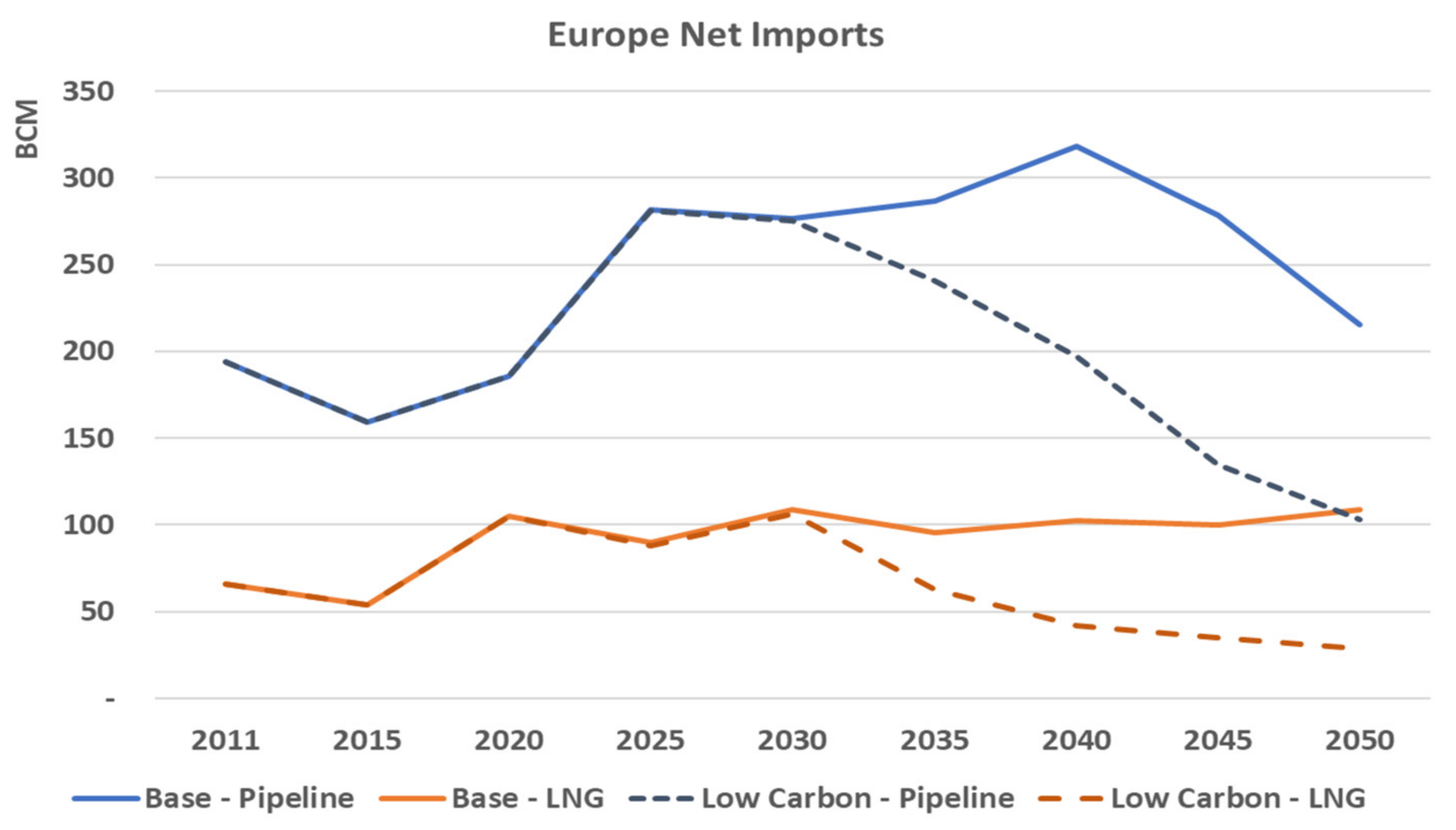
First, due to a lowered demand for natural gas, Europe’s LNG net imports drop by 25%, while pipeline net imports drop by 50%, which is in total a net 190 BCM reduction in imports shown in Figure 23.

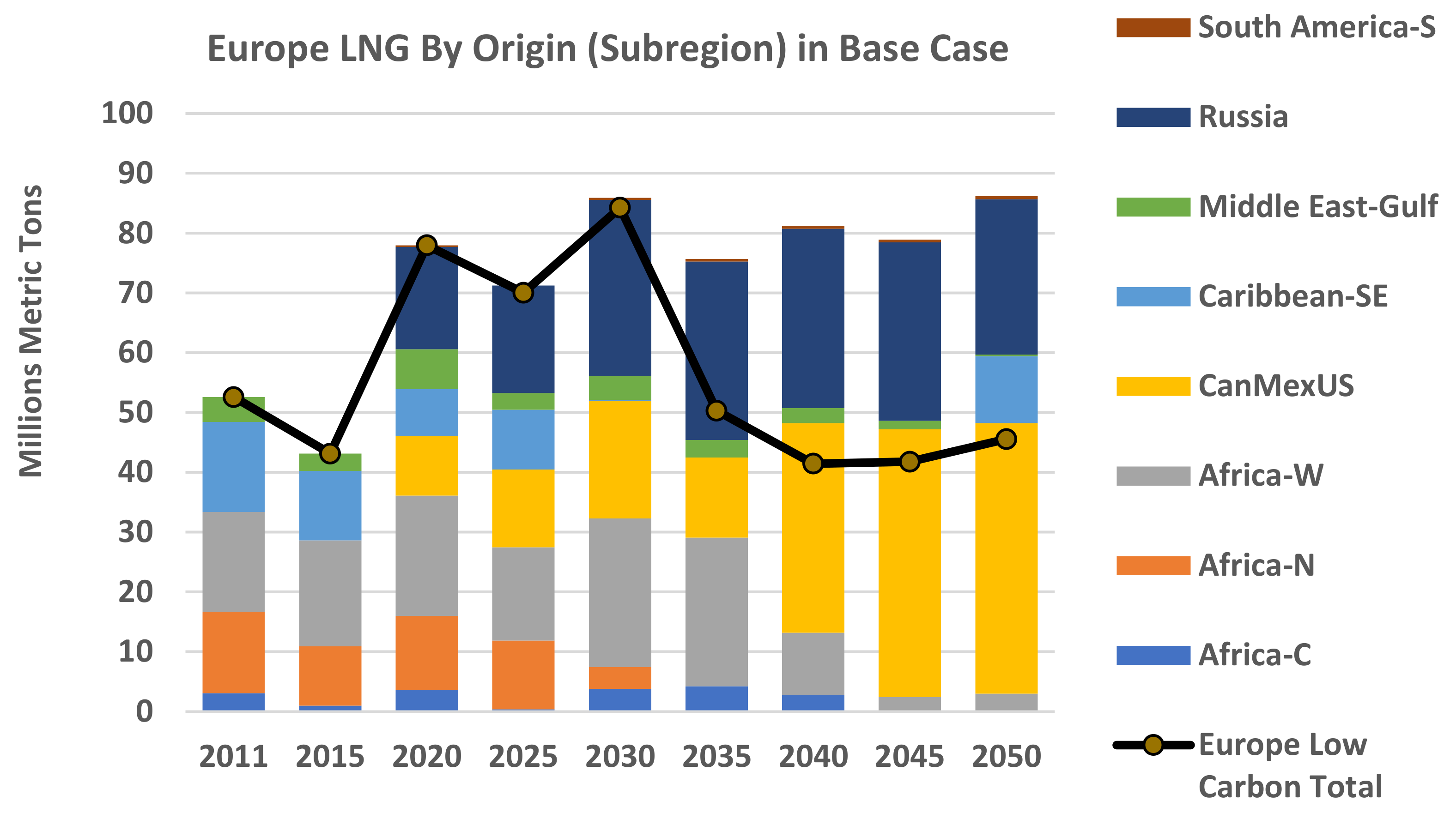
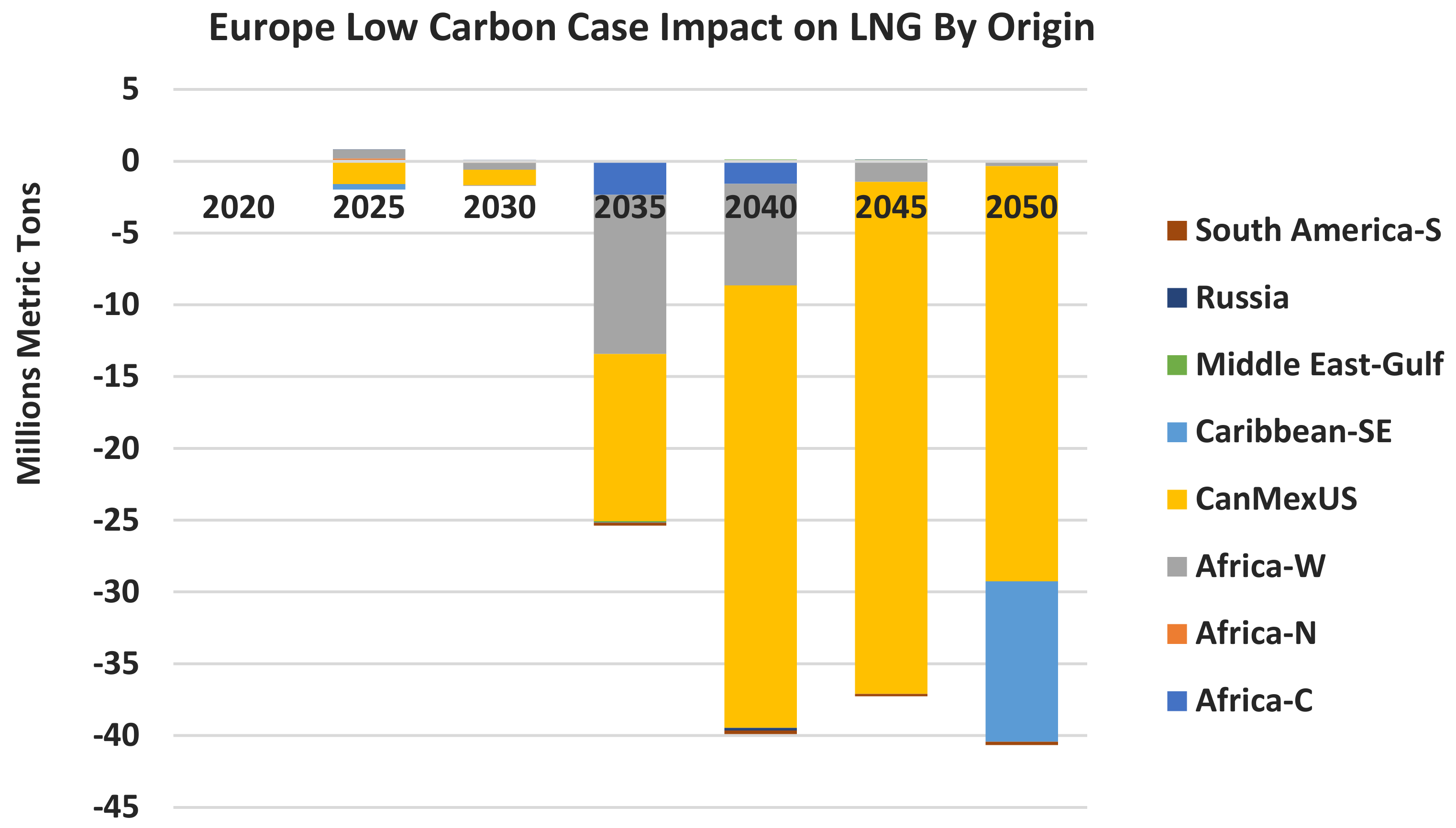
Shown in Figure 24, in the base case, the Europe LNG imports market is expected to grow to around 86 million tons (110 BCM/4.8 tcf) per year by 2050. Europe diversifies its LNG sources from Russia, North America, North and West Africa, and the Middle East. In the low-carbon Europe case, LNG drops about 45 million tons (about 50%) versus the base case in Figure 25. The North America LNG import loses two-thirds of its volume in Europe after 2035.

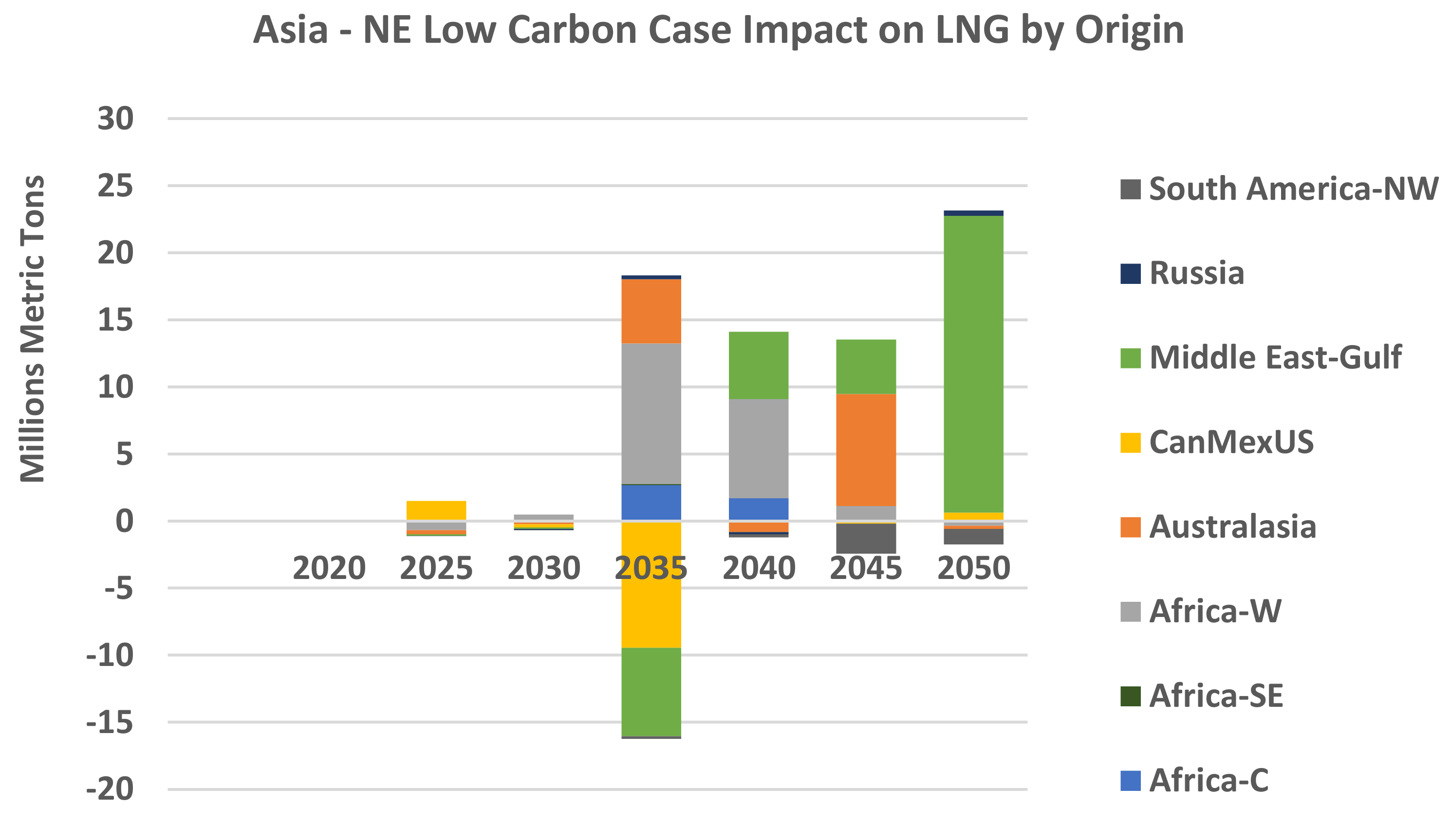
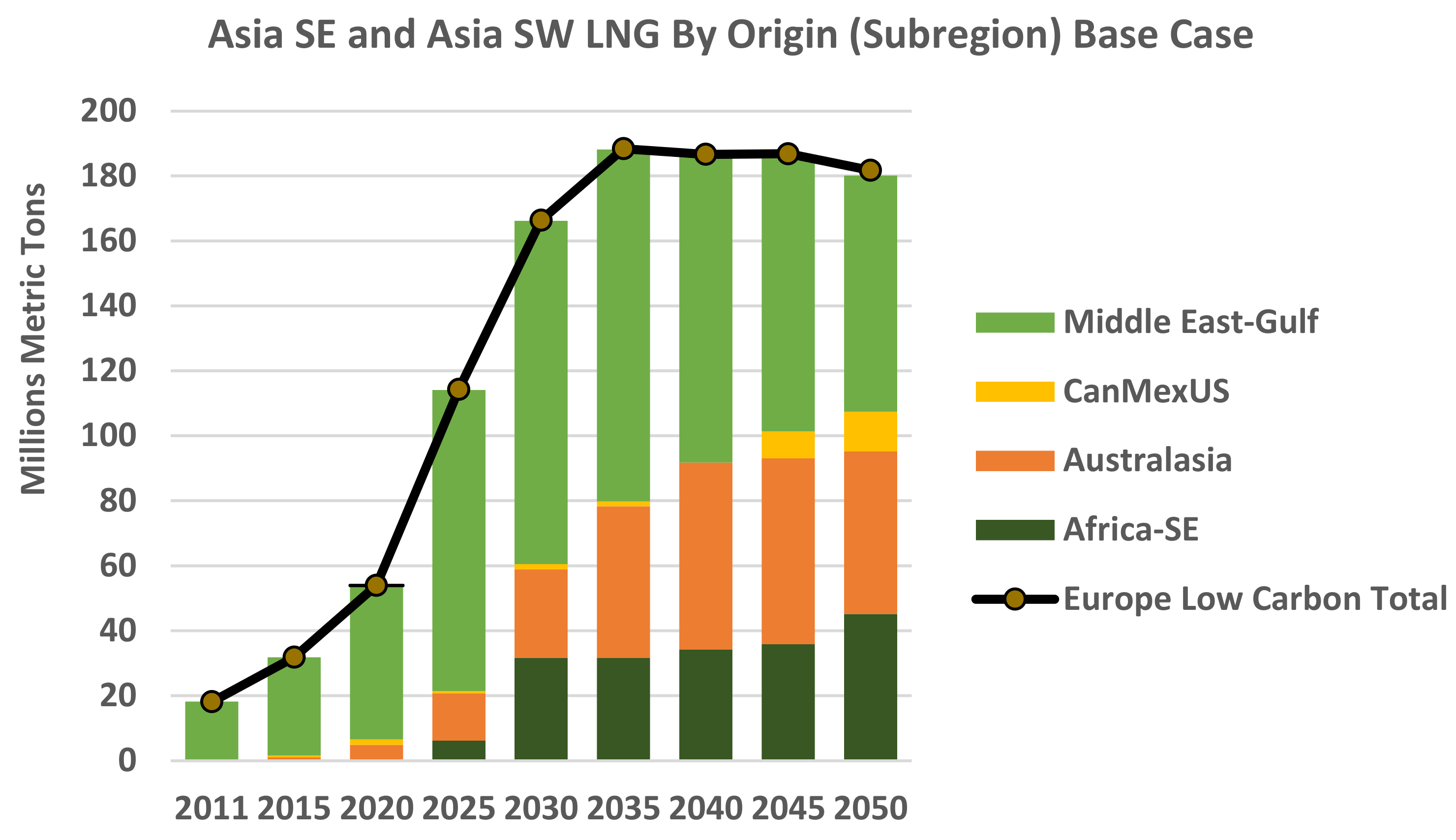
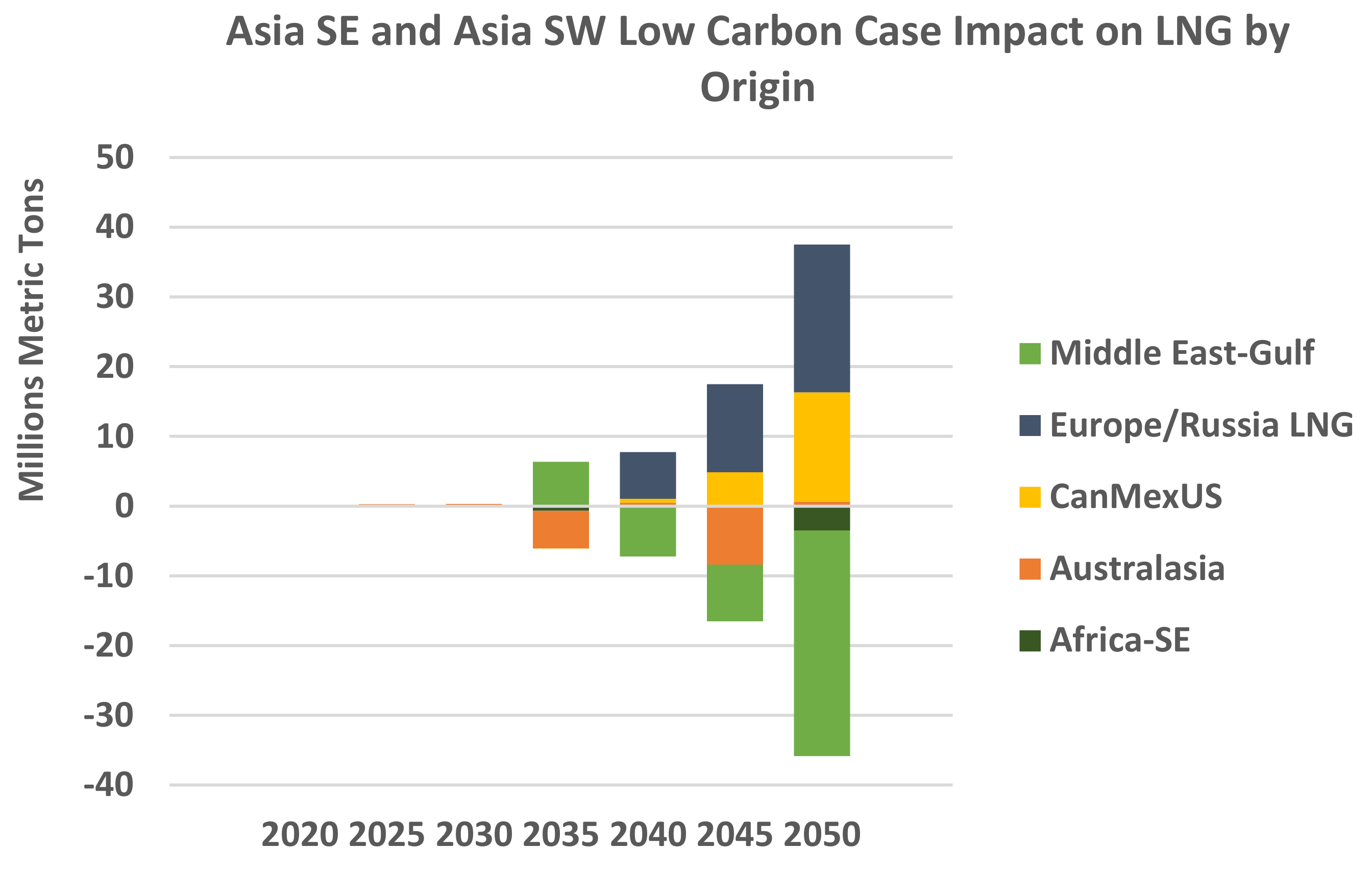
Besides Europe, we go further into the LNG trade differences across each major LNG region. So, moving from Europe to the East, the Southeast and Southwest Asia region has small impacts in terms of total LNG imports as in Figure 26. Due to the changes in Europe here in the base case, the main LNG suppliers are the Middle East and Australia, and then later Africa SE (Mozambique and Tanzania), while in the low-carbon europe case, the Middle East and Australian imports are replaced by LNG from the Russia/European route and North America for a total of about 36 million tons, which is 80% of what is lost in the European market, shown in Figure 27.

Moving further to the east, we arrive at the Northeast Asia region, including four major LNG buyers: Japan, South Korea, China, and Taiwan. As opposed to the SE and SW Asia region, here there is a mild demand response (about 5–7%) in total LNG imported into the Northeast Asia region due to the low gas demand in Europe in the low-carbon case compared to the base case. This implies that the Northeast Asia market is actively competing with the European market on the margin in certain seasons of the year. This is something the market observed in the past.

In the base case, Northeast Asia has a diverse portfolio with cargos from North America, Australia, the Middle East, Russia, and some from Africa. In the low-carbon case, there is a more dynamic change in LNG competition in Northeast Asia presented in Figure 28. The Middle East and Australian imports are pushed back into the Northeast Asia market from the rest of Asia and by some competition with North America. West Africa LNG, which was pushed out of Europe, has largely switched to the Northeast Asia market; there is about 11 million metric tons of LNG reduction by West Africa into Europe in 2035, while a 90% amount is repositioned here into the Northeast Asia market. Second, Australia LNG, which was pushed out in Southeast and Southwest Asia by excess LNG cargo originating in Russia or Europe, finds its way back to the Northeast Asia market with a 12–15% loss in net demand of LNG. West Africa (Nigeria) LNG is redirected from Europe to NE Asia.

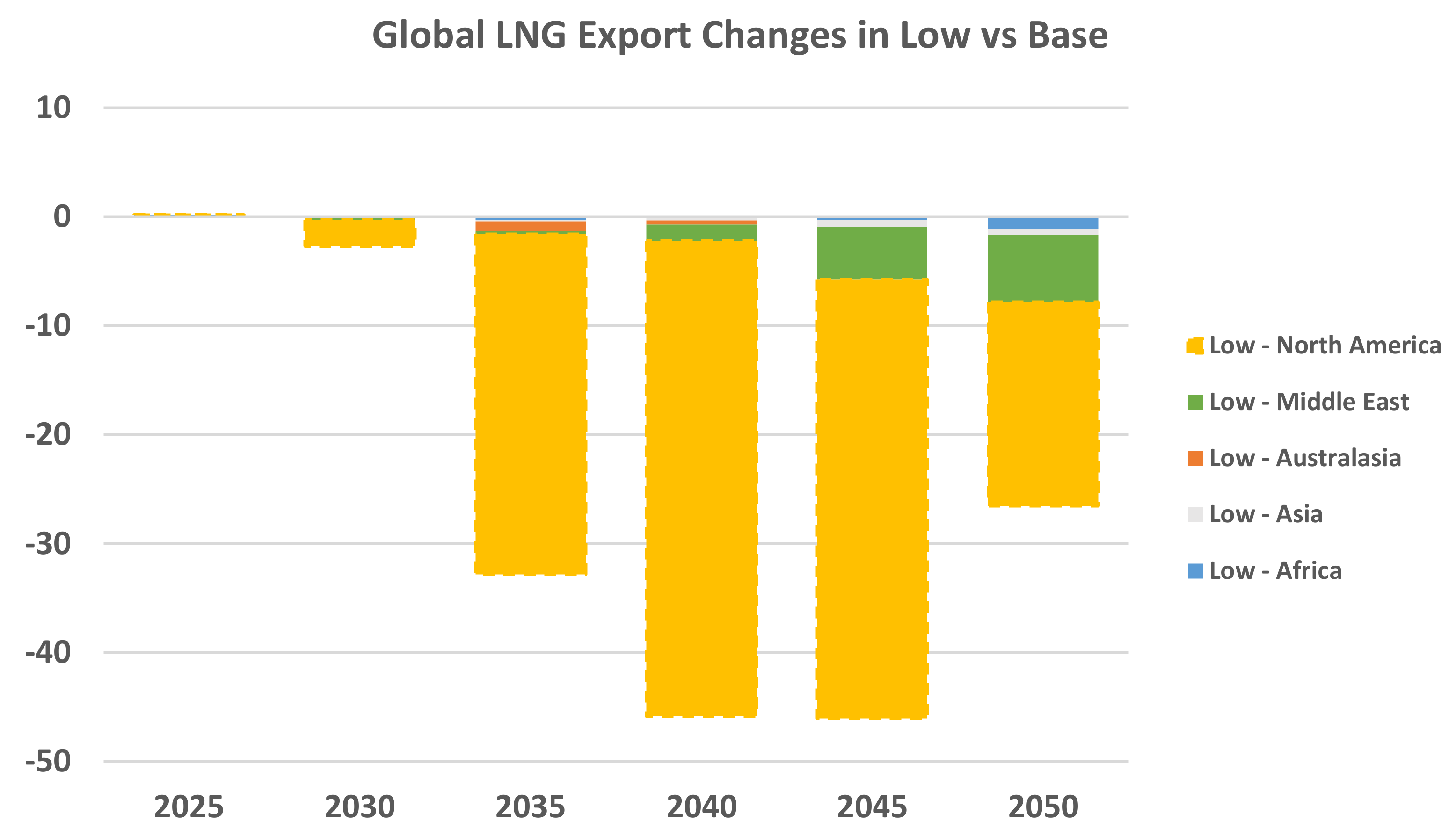
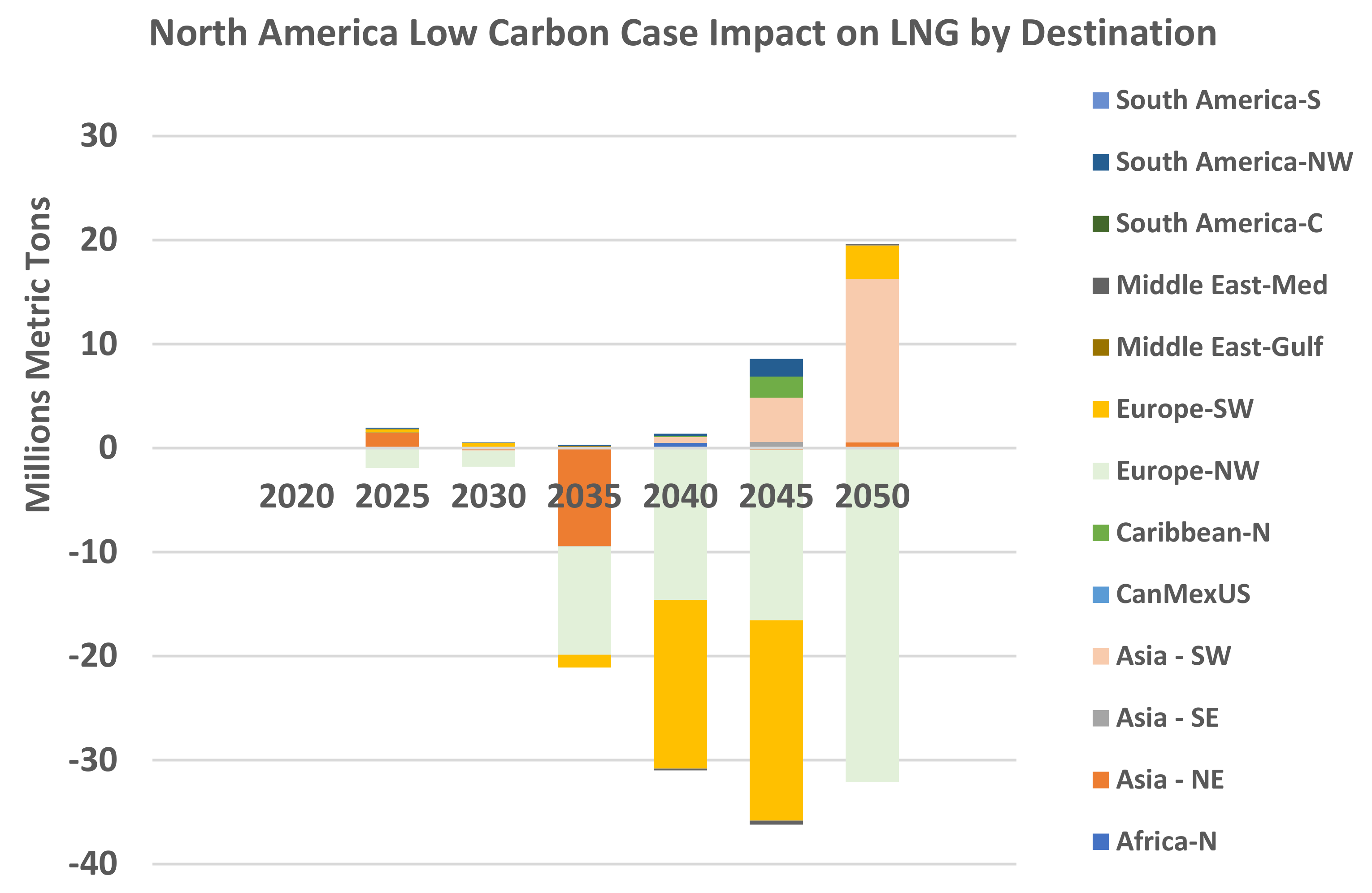
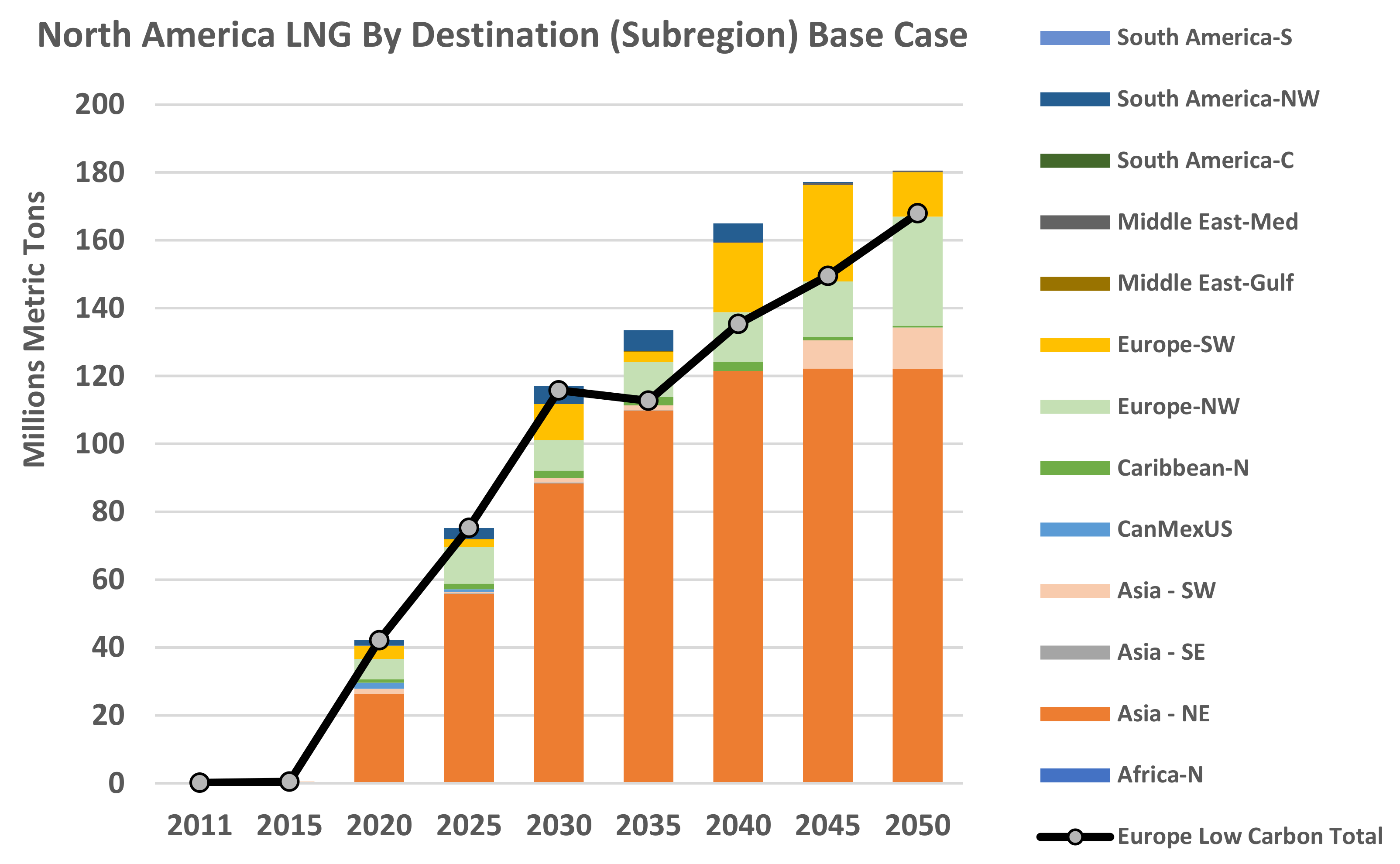
After discussing the impacts for each major LNG-buying region, here are the impacts for each LNG-selling region. With the reduction of LNG demand in Europe—a net of 60 BCM of reduction—the rest of the world managed to balance and reposition about one-third of the reduction mainly to the Asian market, while two-thirds is a net loss of the market due to demand change. Figure 29 shows the export change by origin countries in low carbon case versus base case. For the majority of the demand reduction of LNG, North America seems to receive most of the impact. For example, the largest reduction of LNG trade occurs in 2040–2045, around 45 million metric tons, of which 40 million metric tons is the reduction from North America LNG exports. The Middle East and Australian LNG exports are relatively stable in response to the change in lowered LNG demand in Europe.

In Figure 30, for North America in the base case, LNG exports are expected to grow to 180 million metric tons (8.6 tcf) by 2050, while in the low-carbon Europe case shown in Figure 31, the impact is around 12 million metric tons (0.6 tcf), or less than 10%, as North America would be able to shift most of its lost volume to Southwest Asia, as well as to the Caribbean and South America markets.

7. Summary of Findings and Discussion of Caveats

Modeling regime-switching, such as an energy transition, is of great value to the current industry. It provides long-term and fundamental alternative views—where the differentiated outlooks drive value in terms of providing rationality to formulate strategies under great risks. In this study, we focus on constructing a drastic regime-switching scenario for a low-carbon Europe with a 55% reduction of LNG demand by the year 2050 as a result, and comparing the changes in LNG trade flow by region. This analysis provides insights into potential opportunities and alternative market choices for major LNG exports. U.S. LNG has the most to lose in terms of market share under this scenario, as Russia and Middle East LNG would be shifted to compete in the Asian market due to the reduction of imports into Europe. Asia will have the greatest gain of competitive LNG sources in the long run. This would also likely make LNG projects out of Africa challenging, unless there were more regional LNG demand being developed for the Middle East and African regions.

There are additional market factors that one could consider beyond what is included in the low-carbon scenario in this study. During the energy transition, there are changes across every segment of the natural gas value chain besides demand. For midstream transportation, there could be changes due to the limitation of fuel on the cost of LNG shipping in the long run and emission credit applied for LNG cargo based on the emission factor of its source. Furthermore, with a lower carbon scenario, the changes in the infrastructure of natural gas come mainly from the changes in infrastructure utilization with the risk of stranded or underutilized assets, which include pipelines, underground storage, and terminals. Many pipelines and underground storage owners will start looking into hydrogen or renewable gas sources for additional opportunities. This paper does not discuss the changes in pipeline flow in detail, but that is a topic worth further investigation. The status of some key pipeline development would be an important topic for the stability of the gas market in Europe going forward.

Farther up in the upstream, natural gas producers focus mainly on reducing emissions throughout the operation, and that may drive up the cost of production. Furthermore, there are additional resources that may be put on hold in a lower-demand scenario, with a shorter timeline to fulfill payouts for investments. This can be reflected through a shifting up of the supply curve as the quantity decreases, given the same expected prices.

With all the possible examples of constructing a low-carbon case, one can see the benefits of scenario planning using a structural market model. However, there are several caveats for a structural model under a regime switch, and certain cautions need to be applied in using a model like G2M2^®.

Caveat 1—Data: the principal caveat accompanying this choice of granularity is that not all the desired information is available, and that which is available is often contradicted by similar data from other sources. There is no single global standard for gas production, consumption, and transport for LNG production and trade. One must collect and analyze data from the various sources and develop a system for estimating the historical levels of these quantities, computed so that there is reasonable consistency at the chosen level of granularity and periodicity.

Caveat 2—Economic “Equilibrium” Models vs. Reality: a second caveat is also necessary to mention. G2M2^® is essentially a multi-period partial equilibrium model. “Equilibrium” is meant simply as “supply and demand are in balance” in each period of the simulation. Of course, gas and LNG storage play a role in keeping the market “in balance,” especially for those geopolitical units that have highly seasonal demand. In all such models, there is a basic assumption that there are enough players in the market and enough time to make trades and deals so that, on average, for each period (month) of the simulation, the market is approximately “in balance.” Additionally, of course, the factor that permits or produces this balance is the price. In G2M2^®, prices are computed for every pipeline, storage facility, and LNG terminal in every GPU in every period. Some of these points can be mapped to trading or virtual trading hubs for which historical (and futures) prices are available. Thus, there is information that can be used to help “calibrate” the model’s parameters to more closely approximate the actual activity in gas markets from the past.

When one attempts to replicate what has happened in the past using rational calibration techniques, one finds that a purely economic solution based on the principles described above will inevitably be “better” or “more optimal” or “more economic” than what the historical data shows. Something is missing that keeps the market from behaving in such a hypothetically optimal fashion.

Caveat 3—Uncertainty in General: whether the modeler or analyst is modeling something in the near term or a long way into the future, there are always substantial uncertainties. In the near (and long) term, demand is quite uncertain. This is largely due to its dependence on the weather and the associated difficulty in forecasting weather. Demand is usually modeled to be a function of temperature and precipitation. One can often obtain forecasts of these factors for the next several months, which can be used for short forecasts. However, it is also advisable to conduct sensitivity studies around such variables because of their uncertainty.

In the longer term, demand is usually considered to be related to growth in economic or demographic variables as well as competition with other alternatives fuels or sources of energy and government mandates or targets for emissions reductions. All of these factors have a degree of uncertainty to them. This is why it is usually better to consider a set of assumptions about them as a “scenario” or set of “scenarios” rather than a “forecast.” One should be asking the question: if the following set of assumptions were true, what would be their implications? An energy company, consultant, or government regulator would want to construct and compute a number of such scenarios in order to make proper investments, recommendations, or policy decisions.