Article

Analysis of Modular Stator PMSM Manufactured Using Oriented Steel

1
Department of Electrical Engineering, Michigan State University, East Lansing, MI 48824, USA
2
Manufacturing Systems Research Laboratory, General Motors, Warren, MI 48092, USA
*
Author to whom correspondence should be addressed.
Energies 2021, 14(20), 6583; https://doi.org/10.3390/en14206583
Submission received: 21 September 2021 / Revised: 6 October 2021 / Accepted: 8 October 2021 / Published: 13 October 2021
(This article belongs to the Special Issue Advances in the Field of Electrical Machines and Drives)

Abstract

:
Oriented steel has higher permeability and lower losses in the direction of orientation (the rolling direction) than non-oriented steel. However, in the transverse direction, oriented steel typically has lower permeability and higher losses. The strategic use of oriented steel in a modular Permanent Magnet Synchronous Machine (PMSM) stator can improve machine performance, particularly when compared to a machine designed with non-oriented steel, by increasing both torque and efficiency. Typically, steel manufacturers provide magnetic properties only in the rolling and transverse directions. Furthermore, in modern Finite Element Analysis (FEA) software, the magnetic properties between the rolling and transverse directions are interpolated using an intrinsic mathematical model. However, this interpolation method has proven to be inaccurate; to resolve this issue, an improved model was proposed in the literature. This model requires the magnetic properties of the oriented steel in between the rolling and transverse directions. Therefore, a procedure for extracting the magnetic properties of oriented steel is required. The objective of this work is to propose a method of determining the magnetic properties of oriented steel beyond just the oriented and transverse directions. In this method, flux-injecting probes, also known as sensors, are used to inject and control the flux density in an oriented steel segmented stator in order to extract the properties of the oriented steel. These extracted properties are then used to model an oriented steel modular stator PMSM. The machine’s average torque and core losses are compared with conventional, non-modular, non-oriented steel stator PMSM, and modular, non-oriented steel stator PMSM. It is shown that both the average torque and the core loss of the oriented steel modular stator PMSM have better performance at the selected number of segments than either of the two non-oriented steel stators.

1. Introduction

Improved manufacturing techniques reduce the cost of electrical machines while improving performance. Segmented stators simplify the winding process, thus increasing the slot fill factor and the ease of handling and assembly [1,2]. Segmented stator design also enables the use of different materials for the stator and rotor while reducing waste. As a result, the stator can be built with lower-loss magnetic steel while the rotor is built with materials of higher tensile strength, as required by high-speed operation. Due to the separate production of the rotor and stator laminations, the width of the air gap is no longer determined by the limitations of the punching tool. Hence, the air gap can be further reduced. Additionally, this can increase the torque density of the machine. Faults may lead to adverse effects on the operation of the machine and are dangerous to the system and to human safety [3,4,5,6,7]. High fault tolerance is also achieved in segmented stator construction due to the physical separation of the segments [8]. The construction of the segmented stator also allows for the use of oriented steel that shows superior magnetic properties, higher permeability, and lower core losses in the rolling direction [9,10,11]. Therefore, the proper design of oriented steel segments for the stator construction may lead to the enhanced performance of the machine, along with the other advantages of modular stator construction.
In order to design a machine with the use of oriented steel segments, an accurate modelling of the magnetic properties of the steel is required for numerical simulations. The magnetic properties of oriented steel are distinct in different directions, and knowledge of the magnetic properties of all the directions is required in order to accurately design the machine. However, the magnetic properties of only the rolling and transverse directions are supplied by steel manufacturers. Moreover, in modern FEA software, the magnetic properties of the rolling ( 0 direction) and transverse directions ( 90 direction) of the oriented steel are utilized to interpolate the magnetic properties in between these directions with the use of an internal algorithm. Several techniques have been proposed in the literature to model oriented steel in FEA. In [12], an elliptical model was used to simulate the oriented steel. This method assumes that the permeability of the oriented steel follows an elliptical curve at a given flux density, in the rolling and transverse directions. Therefore, from the BH curves in the rolling and transverse directions, the BH curves for any direction can be interpolated. However, it is shown in [13] that the permeability of the oriented steel is the lowest at around the 50–60 direction, hence the interpolation method using an ellipse is inaccurate. In [14], the magnetic field cross effects using a non-linear method is proposed. The cross field exists when the magnetic field is applied in a direction other than the principal direction, which leads to the non-parallel magnetic field intensity (H) and the flux density (B). However, the cross effects are negligible when the field is applied in the principal direction. In the proposed method, the equivalent magnetic field components are substituted when the cross effects present are derived from the co-energy densities. Using this technique, the equivalent behavior of anisotropic materials can be simulated in any direction. This method has shown improvement in the modelling of the oriented steel over the elliptical. However, in [13], it is shown that variation of the magnetic properties of the oriented steel in between the rolling and transverse directions is unique for every material. Therefore, a mathematical model based on the interpolation of the magnetic properties of the rolling and transverse directions cannot ensure the accuracy of the modelling of the oriented steel. In [15], the reluctivity is modelled as the tensor for the oriented steel. The reluctivity matrix has non-zero, non-diagonal elements that have resulted from the consideration of reciprocal parameters along the principal direction. By choosing the appropriate axis, the tensor matrix is reduced to a diagonal matrix, which predicts the properties of the oriented steel in all the directions between the rolling and the transverse. This method is experimentally validated on a transformer core; however, this method is very complex to apply. In [16], the oriented steel is used to improve the performance of the high-speed traction motor. However, the details of the numerical simulations using FEA is not provided.
In [17], a relatively simple method of modelling a PMSM with an oriented steel modular stator is proposed. The stator is created as a piecewise isotropic model where each isotropic section utilizes the properties of the oriented steel based on the flux flow direction in the stator. This proposed method is based on the fact that flux generally flows radially in the teeth, and then flows circumferentially in the back iron between the adjacent teeth. This modelling method requires the properties of the oriented steel in the direction of each tooth, and the portion of the back iron between two adjacent teeth with respect to the orientation direction. The higher the number of teeth in a stator, the smaller the angular displacement between adjacent teeth. Consequently, a larger number of teeth requires BH and loss curves for more distinct angular orientations with respect to the rolling direction. In such situations, the use of a standard Epstein frame test is expensive and tedious as a lot of the oriented steel sheets that cut along the different directions of orientation are required for testing. Hence, a method that is more practical and comparatively less expensive is required to extract the properties of the oriented steel.
The purpose of this work is to develop a relatively inexpensive method for extracting the properties of the oriented steel relative to the rolling and transverse directions. The idea of the proposed methodology is to develop and use sensors to inject flux of a desired magnitude and frequency into the oriented steel segmented stator. The first contribution provided systematic steps for the acquisition of the properties of a particular oriented steel, which could then be used to design a machine. The obtained magnetic characteristics were used to model an existing PMSM with a modular stator, and the performance of this stator was compared with the same stator using modular and non-modular non-oriented steel. It was observed that the core losses and average torque in the PMSM with an oriented steel modular stator were decreased and increased, respectively, for some specific number of segments as compared to those in the PMSM using both modular and non-modular non-oriented steel stator.
This paper is organized as follows: Section 2 discusses the modelling of anisotropic steel in segmented stators. Section 3 discusses the proposed method for the extraction of magnetic properties of segments. Section 4 describes the experimental set-up, the procedure for the estimation of BH and loss curves of the oriented steel from experiments, and the experimental results. Section 5 makes a comparison of the modular stator PMSM and the PMSM using both modular and non-modular non-oriented steel stators. Section 6 discusses the selection of the number of segments for best performance. Finally, Section 7 draws the conclusions of the paper.

2. Modelling of Anisotropic Steel in the Segmented Stators

Oriented steel (anisotropic steel) has crystal grains oriented in one direction, known as the rolling direction. Due to this internal morphology, the magnetic characteristics of oriented steel depend on the flux direction. Such behavior is different in non-oriented or quasi-isotropic steel, which has almost the same characteristics regardless of the direction. Moreover, anisotropic steel has different BH and loss curves in every direction, unique for every steel, which makes it difficult to model in finite-element simulations. In today’s FEA software, the BH and loss curves of the rolling and transverse directions are used to interpolate the magnetic properties in between these two directions. Moreover, the method of interpolation is not controlled by the user, which may lead to inaccurate results.
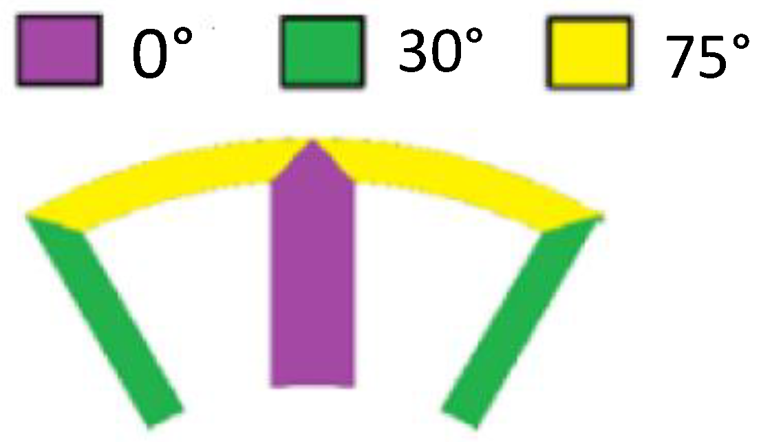
In [17], a method that could be used in FEA to accurately analyze the performance of a PMSM with oriented steel stator laminations was developed. In this method, the stator was divided into sections, and based on the direction of the flux, the BH and loss curves were assigned to individual sections. Thus, the simulation was reduced to a connected structure of isotropic materials. Because of the structure of the proposed model, it is termed here as a piecewise isotropic model. The machine used for analysis in [17] was a 12-slot/14-pole PMSM consisting of six segments where each segment was generally oriented in the direction of the teeth. The direction of orientation of one segment is shown in Figure 1.
For one segment, the direction of flux in the middle tooth is in the direction of alignment, i.e., 0 away from the rolling direction; for the two adjacent teeth, the direction of flux is 30 away from the rolling direction. For the back iron between the middle tooth and the adjacent tooth, the flux changes the direction from 90 to 60 as it flows through the back iron. The proposed model in [17] was obtained by connecting the segments with the BH and loss curves of the 0 direction on the central tooth, and with the BH and loss curves of the 30 direction on the lateral teeth; the back iron was modelled using the BH and loss curves of the 75 direction, which is the average value of the 60 and 90 angles. The model of one segment is given in Figure 2, and six segments connected together along the circumference are used to model the complete machine.
While the properties of the 0 segment are known from the manufacturer’s data sheet, the other two are generally not and must be measured. Moreover, the number of teeth and the segmentation of the stator determine how many different isotropic segments need to be modelled. It is clear that in order to overcome the shortcomings of the current FEA software and accurately model the segmented oriented steel stator, the magnetic properties of the oriented steel in the desired directions are required. A method of extracting these properties is presented in the next section.

3. Proposed Method for the Extraction of the Magnetic Properties of Oriented Steel

The proposed method is applicable to modular stators consisting of circumferential segmentation, as discussed in [2]. This study focuses on machines where the orientation of each segment is in the direction of the teeth, as shown Figure 1, although the proposed method can be expanded to machines in which the orientation is in the direction of the back iron. The core idea of the proposed method is to calculate the core loss and MMF drop at different levels of flux densities and frequencies of the teeth and the back iron segments of the segmented stator, as shown in Figure 2. These values are subsequently used to estimate the BH and Loss curves in between the rolling and transverse directions. A sensor measures the core loss or MMF drop of a portion of the stator, which is the combination of the core loss of the teeth and back iron. Therefore, to calculate the core loss and MMF drop of each tooth and back iron segment, sensors of different spans are used. In this section, the use of oriented steel segmented stators and sensors is first presented, along with the basic idea of the proposed method. Then, the mathematical model is presented in order to determine the core loss and MMF drop in each tooth and back iron segment.

3.1. Basic Idea of the Proposed Method

Consider a machine consisting of an oriented steel modular stator with N t teeth. The adjacent teeth of this machine are located 360 / N t degrees apart, and the steel orientation of these two teeth are also 360 / N t degrees apart. For example, for a 12-slot machine, the two teeth are 30 apart, as shown in Figure 2. As the number of teeth increases, the change in their orientation decreases; hence, data at more discrete orientations are needed to accurately model the machine. This implies that the Epstein frame tests become more impractical as N t increases. In the proposed method, the stator used to measure the magnetic properties should be the same as the final desired stator design, and the number of segments should be chosen to provide enough different orientation angles for the final analysis. This is demonstrated in Figure 3, where the magnetic properties of the teeth and back iron in one segment are shown for a machine consisting of 72 teeth and N s number of segments. Clearly, the machine with N s = 4 can provide magnetic data for the oriented steel at more orientation angles compared to the machine with N s = 6 . The components with similar magnetic properties are similarly coloured.
A common starting point in designing the modular stator is the stator used in its non-modular counterpart [2]. In this work, the geometric design of the stator already used for testing is the initial design of the non-modular stator.
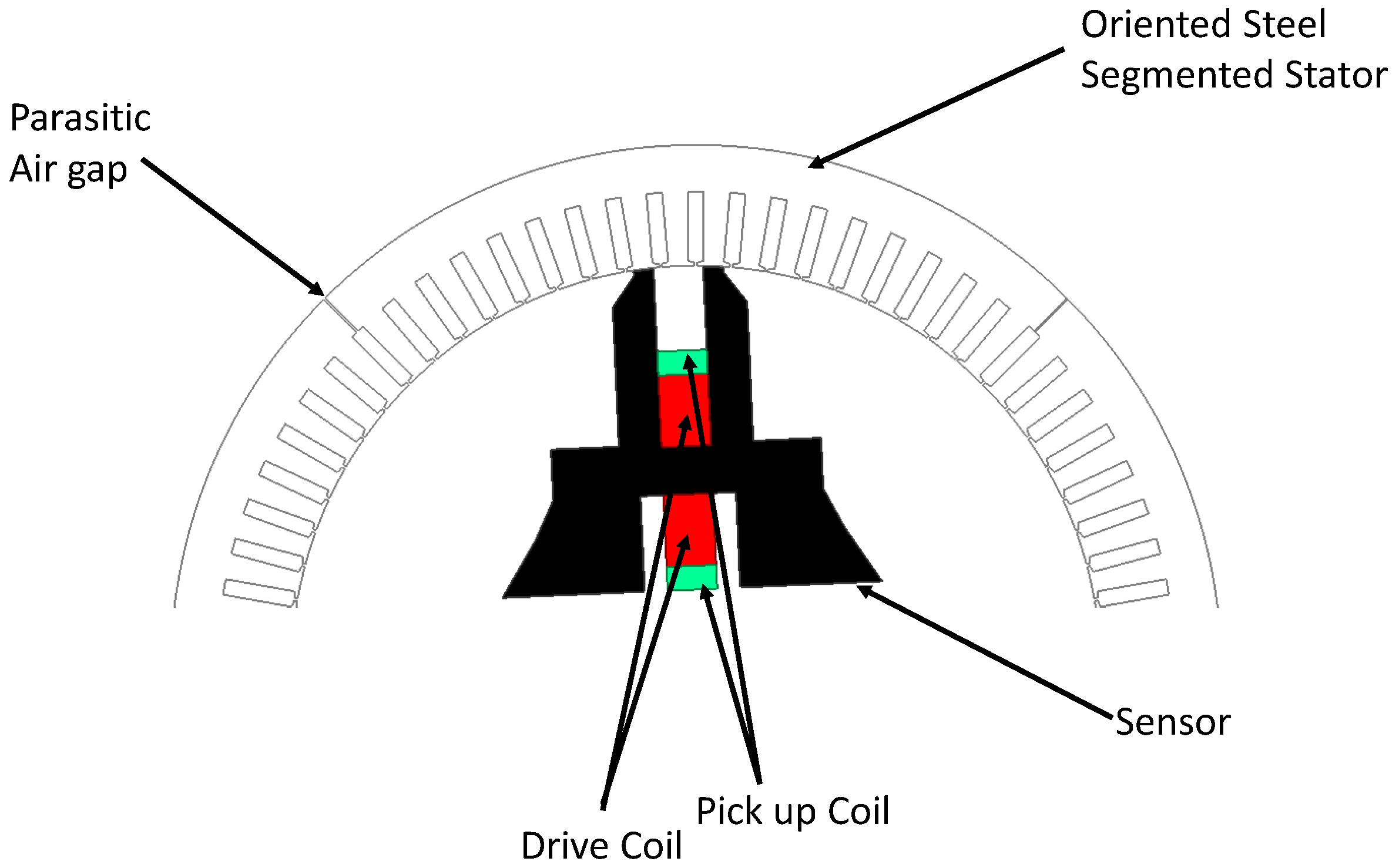
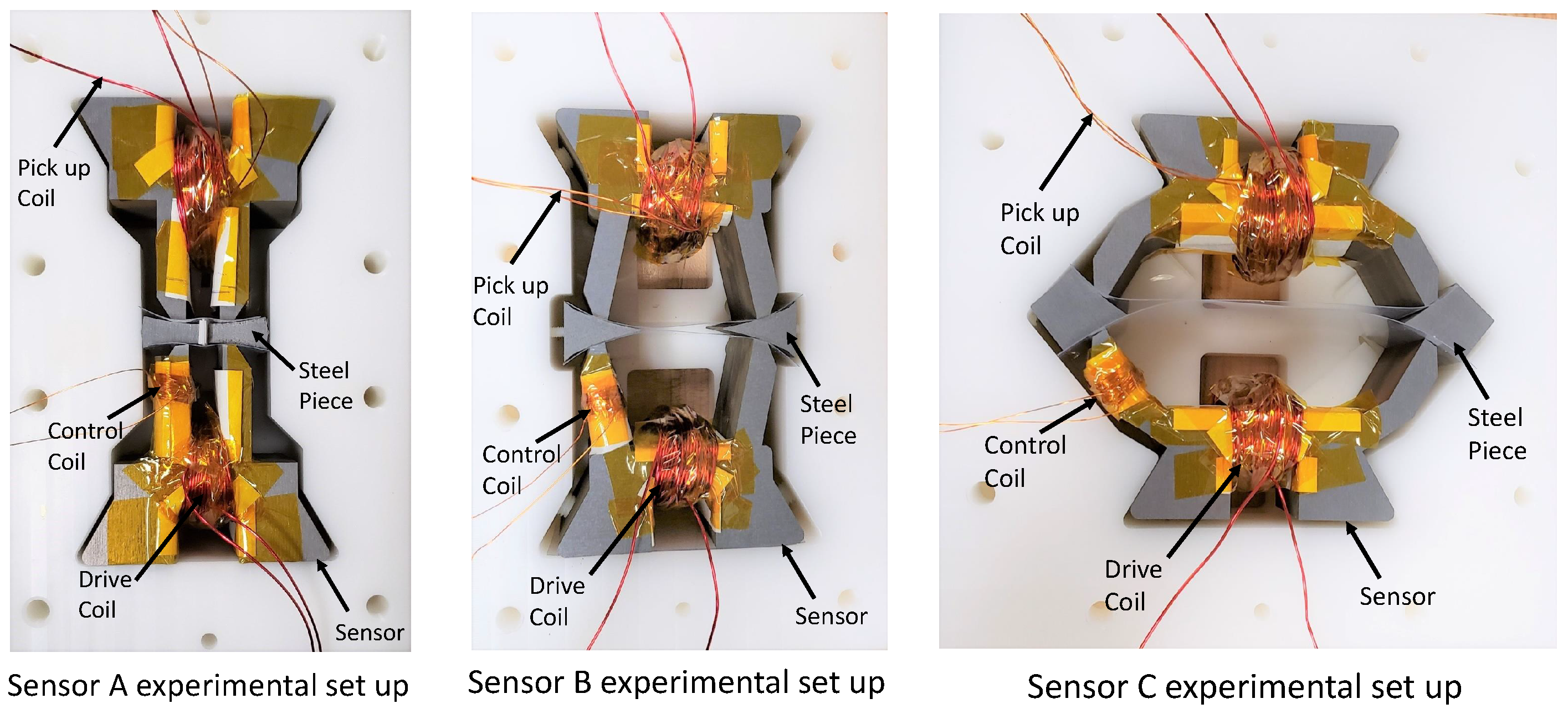
The second requirement of the proposed method is the sensor. The sensor imposes a time-dependent magnetic flux of controlled amplitude and frequency in the stator teeth and back iron. It consists of an H-shaped core of high-quality magnetic steel laminations and two coils: a drive coil to impose a current and the resulting magneto motive force (MMF) onto the circuit, and a pickup coil to measure the induced voltage. Figure 4 shows the experimental set-up consisting of oriented steel stator and sensor, indicating the drive coil or primary coil and the pick-up coil or secondary coil.
The motivation to use sensors such as these to inject the flux into the stator is to emulate the direction of flux in the stator teeth and back iron, similar to that during machine operation. The applied flux passes through the teeth, follows the path from the back iron spanned by the sensor, and then returns through the second tooth opposite to the second sensor limb. The teeth directly in line with the sensor limbs provide the properties of the oriented steel in the orientation of the said teeth. The same is true for the portion of the back iron in between the adjacent teeth. A third component is the flux in the outer portions of the teeth between the sensor limbs, but this is not used for analysis due to the non-uniformity of the flux flow in these regions. The flux lines in the portion of the segment injected by the sensor that spans over one tooth with the orientation angle is shown in Figure 5. The relative placement of the teeth for this example is 5 .
The flux in the pink and green teeth emulates the flux of the machine teeth under operation. Similarly, the red and orange components of the back iron emulates the flux of the machine back under operation. As discussed in Section 2, the pink teeth, green teeth, red back iron, and orange back iron represent the magnetic properties of 0 , 10 , 87 . 5 , and 82 . 5 away from the rolling direction. However, due to the non-uniformity of the flux in the yellow portion, the magnetic properties in those teeth cannot be determined with confidence. Therefore, in this work, the magnetic properties of these components are not used to estimate the magnetic properties of the oriented steel. The core losses or MMF drops measured by the sensors are denoted by “Y”. Hence, the core losses or MMF drops measured by the sensor from Figure 5 is calculated as follows:
Y sensor = Y Pink Teeth + Y Green Teeth + Y Red Back Iron + Y Orange Back Iron + Y Yellow Portion
In this work, the back iron, teeth, and the teeth with non-uniform flux are denoted by X, T, and T ^ , respectively. Thus, Equation (1) is reduced to:
Y sensor = Y T 0 + Y T 10 + Y X 87 . 5 + Y X 82 . 5 + Y T ^ 5
where the angles in the suffix show the magnetic properties X or T. Notice that for T ^ , the suffix is denoted by 5 just to indicate the location of T ^ with respect to the orientation direction. The sensors are used to measure the core losses and MMF drops at different values of flux densities and frequencies at different positions in the stator. For the values of the flux density and frequency, the values of the core loss and MMF drop for each X and T are calculated and then finally used to estimate the core loss and BH curves.
In order to calculate the core loss or MMF drop of X and T, the sensors of different spans are used. The measured values of core losses and MMF drops at different positions, from different sensors, within the oriented steel stator are represented by a set of linear equations. These equations are solved, and the values of the MMF drops or the core losses of individual teeth and back iron are obtained. The number and span of sensors required to achieve this depend on the number of segments and the number of teeth in the oriented steel stator used for testing. The selection of span and number of sensor is illustrated by an example.
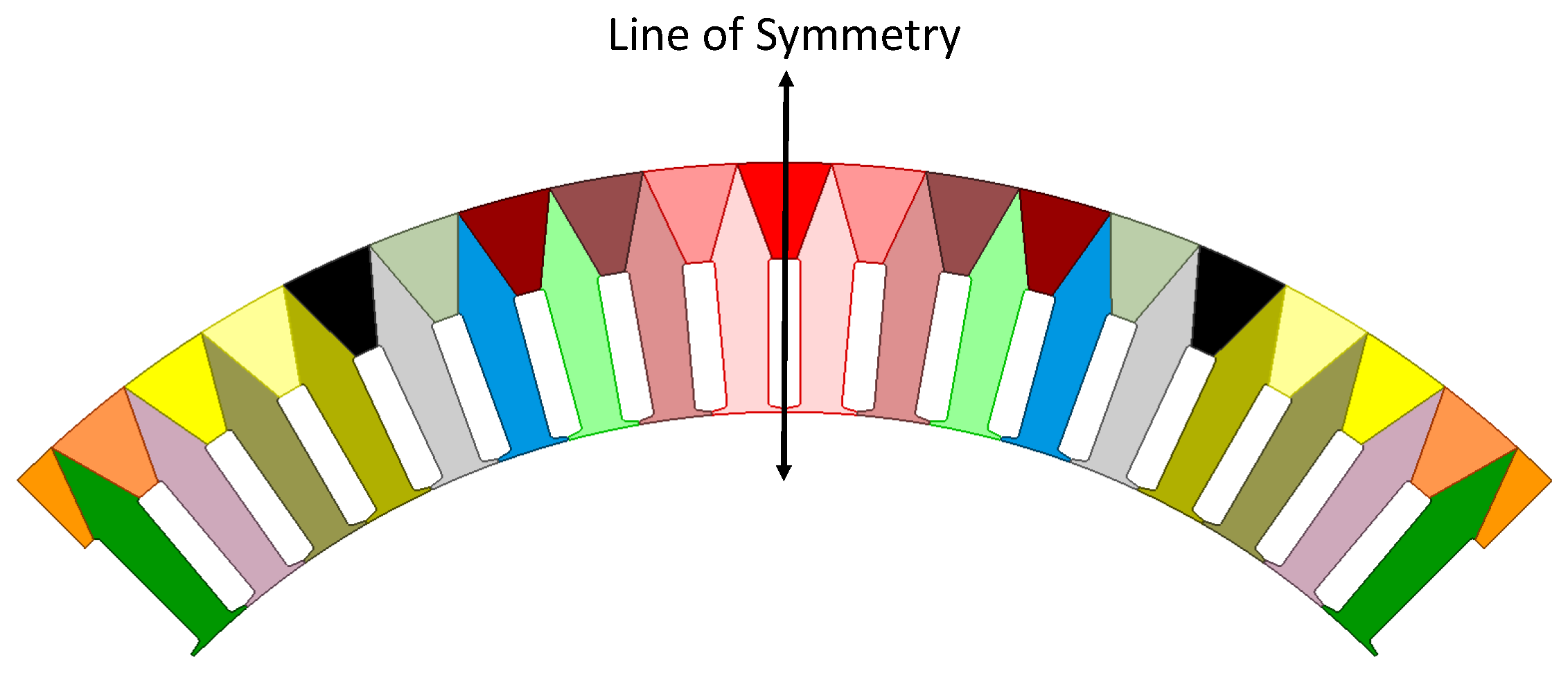
Suppose one of the segments consists of an even number of teeth, denoted by “n”. Each segment of the stator is symmetric along the axis that divides the segment into two identical parts. Figure 6 shows the line of symmetry, and all the components are coloured the same to represent identical magnetic properties.
This means there are n/2 different T and T ^ , and n/2 + 1 different X that may show different values of core losses or MMF drops for the same values of flux density and frequency. This results in 3n/2 + 1 variables to be solved with different spans and numbers of sensors. The sensor spanning over an odd number of teeth provides n/2 unique equations of the combinations of all three components, while the sensor spanning over an even number of teeth provides n/2 + 1 unique equations. These are obtained when the sensor measures the core losses or MMF drops in the stator at different positions. These equations, when combined, may not yield a total of 3n/2 + 1 unique equations. However, it can be shown that these equations can be solved with the use of simple assumptions. This implies that a combination of two sensors spanning an odd number of teeth and one sensor spanning an even number of teeth can be used to obtain the values of all the components. For the sake of simplicity, the measured core losses or MMF drops, which are the linear combinations of the three components, are arranged in the form of the matrices:
Y o d d s e n 1 n 2 × 1 = A o d d s e n 1 n 2 × 3 n + 2 2 × K 3 n + 2 2 × 1
Y o d d s e n 2 n 2 × 1 = A o d d s e n 2 n 2 × 3 n + 2 2 × K 3 n + 2 2 × 1
Y e v e n s e n n + 2 2 × 1 = A e v e n s e n n + 2 2 × 3 n + 2 2 × K 3 n + 2 2 × 1
where vector Y consists of the measured values at different sensor positions, matrix A accounts for the number of times each discrete steel orientation angle appears in the sensor span, and vector K represents the core losses or MMF drops of all three components. The same discussion can be extended to measurements with a sensor spanning an odd number of teeth. The application of the proposed method is discussed in the next section.

3.2. Application of the Proposed Method

The stator used for testing had 72 teeth, and the selected number of segments was four. Four segments were selected to extract data at all angles away from the rolling direction in 5 steps, as shown in Figure 3. Therefore, the information extracted from the four segments could still be used to model a machine consisting of two or three segments. The three designed sensors were named Sensor A, B, and C. The spans for the three different sensors are as follows:
  • Sensor spans one tooth in stator (Sensor A);
  • Sensor spans six teeth in stator (Sensor B);
  • Sensor spans thirteen teeth in stator (Sensor C).
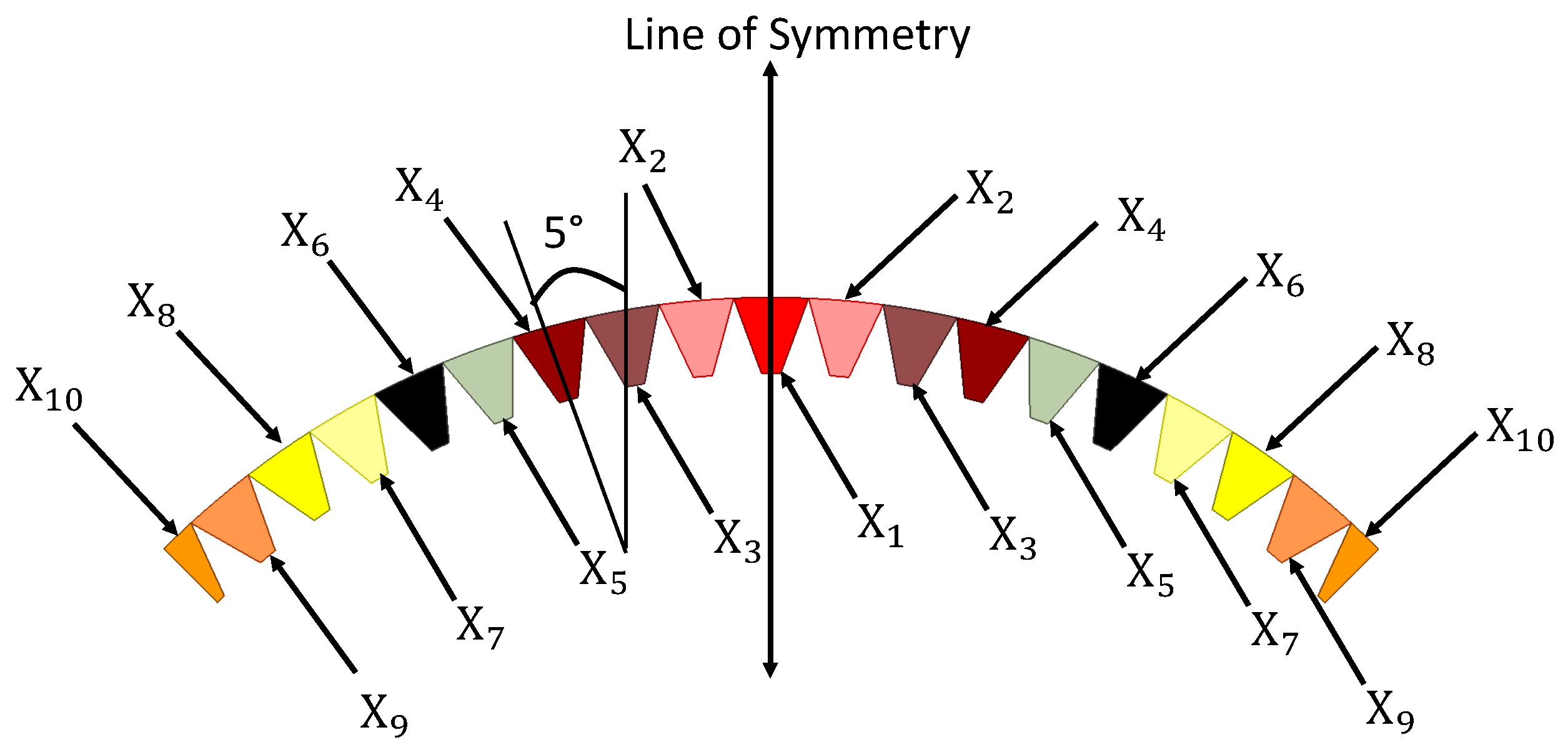
The back iron division with respect to the line of symmetry is shown in Figure 7. The pairs of X i , ∀ i [ 2 , 10 ] , are aligned identically with respect to the rolling direction, and hence they have similar magnetic properties. Moreover, X 1 represents the properties of 90 away from the rolling direction, X 2 represents properties of 85 away from the rolling direction, and so on.
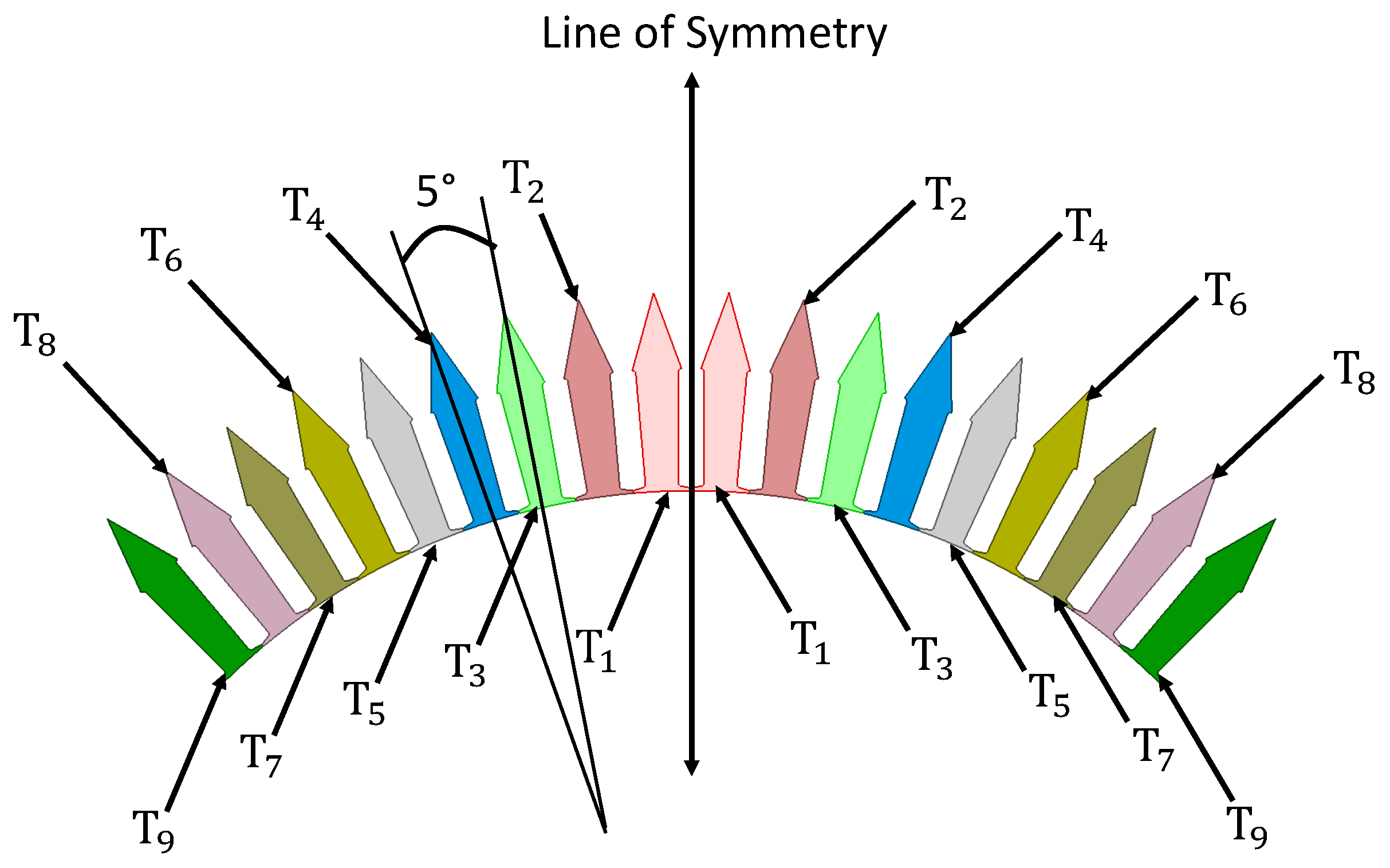
The placement of the teeth with respect to the line of symmetry is shown in Figure 8. The pairs of T j , ∀ j [ 1 , 9 ] , have identical magnetic properties due to symmetry. Moreover, T 1 represents the property of 2 . 5 away from the rolling direction, T 2 represents the property of 7 . 5 away from the rolling direction, and so on. Similarly, symmetry holds for T j ^ .
The lower values of i and j correspond to the positions of X i , T j , or T j ^ on the symmetrical axis, as shown in Figure 7 and Figure 8. Starting from 1, the value of i increases by 1 for every 5 shift. Each sensor is used to measure the core losses and the MMF drops of different pieces of the segmented stator at different positions in the stator. To denote the position of the sensor, the following nomenclature is used:
  • The symmetric placement of the sensor is denoted by “ Sensor name 1 ”. For example, for sensors A, B, and C the symmetric placement of sensors with respect to the symmetrical line are denoted by A 1 , B 1 , and C 1 , respectively;
  • The second position of the sensor is its 5 anti-clockwise shift from position 1. For sensors A, B, and C, these positions are denoted by A 2 , B 2 , and C 2 , respectively;
  • Similarly, the third position of the sensor is its 10 anti-clockwise shift from position 1.
Positions A 1 and A 2 in Figure 9 show how the position of the sensor with respect to the stator is denoted in this method.
The core losses or MMF drops measured by the sensors are denoted by “Y”. Therefore, the core losses or MMF drops measured in a symmetrical position using sensor A are denoted by Y A 1 . Similarly, the core losses or MMF drops of element X 1 are denoted by Y X 1 , and so on. Therefore, the loss measured by sensor A in position A 1 , as shown in Figure 9, is written as the sum of five components:
Y A 1 = Y X 1 + Y X 2 + Y T 1 ^ + Y T 1 + Y T 2
This method divides the core losses or MMF drops in one portion of the segmented stator into the three components, as presented in Equation (6). Using these equations, the core losses and MMF drops for all values of X i , T i and T i ^ are determined. For convenience, equations are arranged in the form of matrices. The equations in matrix form for sensors A, B, and C are given as follows:
Y A 1 Y A 2 Y A 3 Y A 4 Y A 5 Y A 6 Y A 7 Y A 8 Y A 9 = 1 1 0 0 0 0 0 0 0 0 1 1 0 0 0 0 0 0 0 1 0 0 0 0 0 0 0 0 0 1 1 0 0 0 0 0 0 0 1 0 1 0 0 0 0 0 0 0 1 0 0 0 0 0 0 0 0 0 1 1 0 0 0 0 0 0 0 1 0 1 0 0 0 0 0 0 0 1 0 0 0 0 0 0 0 0 0 1 1 0 0 0 0 0 0 0 1 0 1 0 0 0 0 0 0 0 1 0 0 0 0 0 0 0 0 0 1 1 0 0 0 0 0 0 0 1 0 1 0 0 0 0 0 0 0 1 0 0 0 0 0 0 0 0 0 1 1 0 0 0 0 0 0 0 1 0 1 0 0 0 0 0 0 0 1 0 0 0 0 0 0 0 0 0 1 1 0 0 0 0 0 0 0 1 0 1 0 0 0 0 0 0 0 1 0 0 0 0 0 0 0 0 0 1 1 0 0 0 0 0 0 0 1 0 1 0 0 0 0 0 0 0 1 0 0 0 0 0 0 0 0 0 1 1 0 0 0 0 0 0 0 1 1 0 0 0 0 0 0 0 0 1 · K
where K is a column vector given by:
K T = [ Y X 1 Y X 2 Y X 3 Y X 4 Y X 5 Y X 6 Y X 7 Y X 8 Y X 9 Y X 10 Y T 1 Y T 2 Y T 3 Y T 4 Y T 5 Y T 6 Y T 7 Y T 8 Y T 9 Y T 1 ^ Y T 2 ^ Y T 3 ^ Y T 4 ^ Y T 5 ^ Y T 6 ^ Y T 7 ^ Y T 8 ^ Y T 9 ^ ]
Similarly for sensor B and sensor C, the two matrices are given as follows:
Y B 1 Y B 2 Y B 3 Y B 4 Y B 5 Y B 6 Y B 7 Y B 8 Y B 9 Y B 10 = 1 2 2 2 0 0 0 0 0 0 0 0 0 2 0 0 0 0 0 2 2 2 0 0 0 0 0 0 1 2 2 1 1 0 0 0 0 0 0 0 1 0 1 0 0 0 0 2 2 1 1 0 0 0 0 0 1 2 1 1 1 1 0 0 0 0 0 1 0 0 0 1 0 0 0 2 1 1 1 1 0 0 0 0 1 1 1 1 1 1 1 0 0 0 1 0 0 0 0 0 1 0 0 1 1 1 1 1 1 0 0 0 0 1 1 1 1 1 1 1 0 0 1 0 0 0 0 0 0 1 0 0 1 1 1 1 1 1 0 0 0 0 1 1 1 1 1 1 1 0 0 1 0 0 0 0 0 0 1 0 0 1 1 1 1 1 1 0 0 0 0 1 1 1 1 1 1 1 0 0 1 0 0 0 0 0 1 0 0 0 1 1 1 1 1 1 0 0 0 0 1 1 1 1 1 2 0 0 0 1 0 0 0 1 0 0 0 0 0 1 1 1 1 2 0 0 0 0 0 1 1 1 2 2 0 0 0 0 1 0 1 0 0 0 0 0 0 0 1 1 2 2 0 0 0 0 0 0 1 1 2 2 0 0 0 0 0 2 0 0 0 0 0 0 0 0 0 2 2 2 · K
Y C 1 Y C 2 Y C 3 Y C 4 Y C 5 Y C 6 Y C 7 Y C 8 Y C 9 = 1 2 2 2 2 2 2 1 0 0 0 0 0 0 0 0 1 1 0 2 2 2 2 2 2 1 0 0 1 2 2 2 2 2 1 1 1 0 0 0 0 0 0 1 0 0 1 2 2 2 2 2 1 1 1 0 1 2 2 2 2 1 1 1 1 1 0 0 0 0 1 0 0 0 1 2 2 2 2 1 1 1 1 1 1 2 2 2 1 1 1 1 2 1 0 0 0 1 0 0 0 1 0 2 2 2 1 1 1 1 1 2 1 2 2 1 1 1 1 2 2 1 0 0 1 0 0 0 1 0 0 2 2 1 1 1 1 1 2 2 1 2 1 1 1 1 2 2 2 1 0 1 0 0 0 1 0 0 0 2 1 1 1 1 1 2 2 2 1 1 1 1 1 2 2 2 2 1 1 0 0 0 1 0 0 0 0 1 1 1 1 1 2 2 2 2 0 1 1 1 2 2 2 2 2 1 1 0 0 1 0 0 0 0 0 0 1 1 1 2 2 2 2 2 0 0 1 2 2 2 2 2 2 1 0 1 1 0 0 0 0 0 0 0 0 1 2 2 2 2 2 2 · K
All the equations given in (7)–(9) are used to calculate the values of Y X i and Y T i .

4. Experimental Set-Up, Estimation of BH and Loss Curves, and Experimental Results

4.1. Experimental Set-Up

All the sensor limbs are identical, while the control coil voltage, a wound on the sensor limb, is maintained as a sinusoidal signal. The amplitude of the control coil voltage is adjusted by modifying the primary supply voltage, as discussed in [18], in order to obtain the desired flux density in the sensor limb ( B ^ l i m b ). The sensor measures the total MMF drop of the sensor stator arrangement consisting of a portion of the segment, the sensor itself, and the air gaps between the sensor limb and the stator tooth. It also measures the total core loss of the sensor and the corresponding portion of the segment. To calculate the MMF drop/core loss of the portion of the stator segment, the MMF drop of the sensor and the air gaps/core loss of the sensor is subtracted. The MMF drop/core loss of the sensor and the two air gaps/sensor are calculated by measuring the MMF drop and core loss of two identical sensors placed head, on as shown in Figure 10. Both the primary windings are excited with the same primary current to obtain the desired flux density ( B ^ l i m b ) in the sensor limb. The total MMF drop of the set-up consists of two sensors and four air gaps, each with a piece of steel and a sensor limb, and the total core loss of two sensors. Hence, the MMF drop/core loss of the sensor and two air gaps are half of the total. The error due to the presence of a piece of steel in the estimation of core losses and MMF drops is reduced to an acceptable limit by making the area of the piece of steel large enough such that the flux density is small.
The experimental set-up consisting of a sensor and an oriented steel segmented stator is shown in Figure 11. A two-sensor arrangement, shown in [19], is used for testing to avoid flux leakage through the back iron.
The drive coil voltage is applied through the amplifier, while the control coil voltage, pick-up voltage, and primary current are recorded using LabVIEW through an SCB box from National Instruments. The overall experimental set-up consisting of a computer that controls LabVIEW, which is used to send and receive signals from the SCB box, and the amplifier that supplies voltage to the drive coil, is shown in Figure 12.

4.2. Procedure for the Estimation of BH and Loss Curves of the Oriented Steel

The equations discussed in Section 3 are used to calculate the values of the core losses and MMF drops of X i and T i at selected values of flux density and frequencies, as shown in Table 1.
The core loss for each field intensity (H) and orientation angle is calculated using the core loss and MMF drop values of X i and T i , combined with the data supplied by the manufacturer for the rolling and transverse directions. Section 2 shows that X 1 represents the properties of 90 away from the rolling direction, and X 2 represents the properties of 85 away from the rolling direction, and so on. For a given value of flux density and frequency, the % change in core loss of X i with X i is as follows:
Δ x i = Y X i Y X 1 Y X 1 · 100
Since X 1 is oriented at 90 away from the rolling direction, the core loss density (in W/m 3 ) in the transverse direction for the same value of flux density and frequency, denoted by Y t r a n s v e r s e , is used to calculate the core loss corresponding to the angle of orientation of X i . For example, the value of Y 85 is calculated using the following:
Δ x 2 = Y X 2 Y X 1 Y X 1 · 100 = Y 85 Y t r a n s v e r s e Y t r a n s v e r s e · 100
Therefore, the estimated value of core loss (in W / m 3 ) for the 85 angle away from the rolling direction, at a given value of flux density and frequency, is as follows:
Y 85 = Δ x 2 + 100 100 · Y t r a n s v e r s e
The same process is repeated for all the values of X i , at all values of flux densities and frequencies, in order to obtain the core losses for the values of orientation from 85 to 45 . Moreover, using the MMF drop values of X i from the process discussed above, and using the value of H (in A/m) from the transverse direction, flux data are generated. Finally, the core loss and MMF drop values of T i with T 1 are used to estimate the core loss and BH curves for all the orientation angles between 0 and 40 .

4.3. Experimental Results

The estimated BH and loss curves were obtained from the core loss and MMF drop values of X i and T i using the analysis discussed in Section 4.2. It was observed that at 55 away from the rolling direction had highest core losses, while the lowest losses were in the rolling direction. This is a long-known result and proves the correctness of the proposed method. However, for the FEA-interpolated curves, the rolling direction had the lowest losses, and the transverse direction had the highest losses. The core loss curves obtained from the analysis of the experimental results and the FEA-interpolated core loss curves with a supply frequency of 50 Hz are shown in Figure 13.
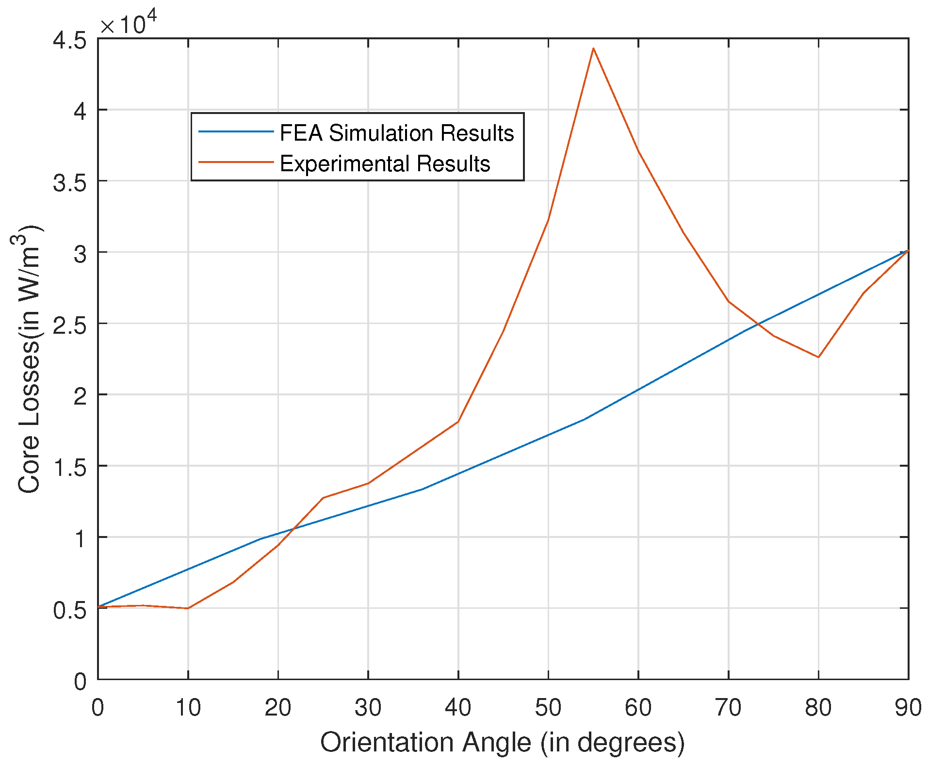
The variation of the core loss curves, with the orientation angle obtained from the analysis of experimental results and the FEA-interpolated core loss curves for 1.5 T and a supply frequency of 50 Hz, is shown in Figure 14. This variation shows the difference between the interpolated properties of the oriented steel in the FEA (the conventional method) compared to the actual properties of the oriented steel obtained from the experiments. This shows the importance of the proposed method in obtaining the characteristics of oriented steel, for the correct modelling of the oriented steel modular PMSM.

5. Analysis of Oriented Steel Modular Stator PMSM

In this section, the BH and loss curves that were obtained from the analysis of experimental results are used in the piecewise isotropic model, discussed in Section 2, are used to model an oriented steel segmented stator. The oriented steel has the lowest core loss and the highest permeability along the rolling direction, while losses are the highest and permeability the lowest along the 55 direction, as shown in Figure 14.
This implies that building the whole stator with a single sheet of oriented steel will not lead to the proper utilization of its magnetic properties. Therefore, a segmented-stator PMSM with different numbers of segments, where segmentation is performed along the slot in the circumferential direction, is used for analysis. Moreover, the effect of increased cut edges, discussed in [2], on the performance of the machine is not studied in this work. The analysis is performed on the 12-pole, 72-slot PMSM. The selected orientation direction of each segment is along the general direction of the teeth, i.e., the center tooth is at 0 . This orientation direction is selected because the flux density in the teeth is higher than in the back iron. One problem with segmented stators is the presence of unavoidable gaps between the segments, also known as parasitic gaps. Parasitic gaps reduce the total flux in the machine, leading to a reduced average torque, and the effect increases with the number of segments. Conversely, as the number of segments increases, the magnetic properties of the teeth improves on average. The purpose of this analysis is to find the best possible number of segments in order to minimize the core losses and maximize the average torque.
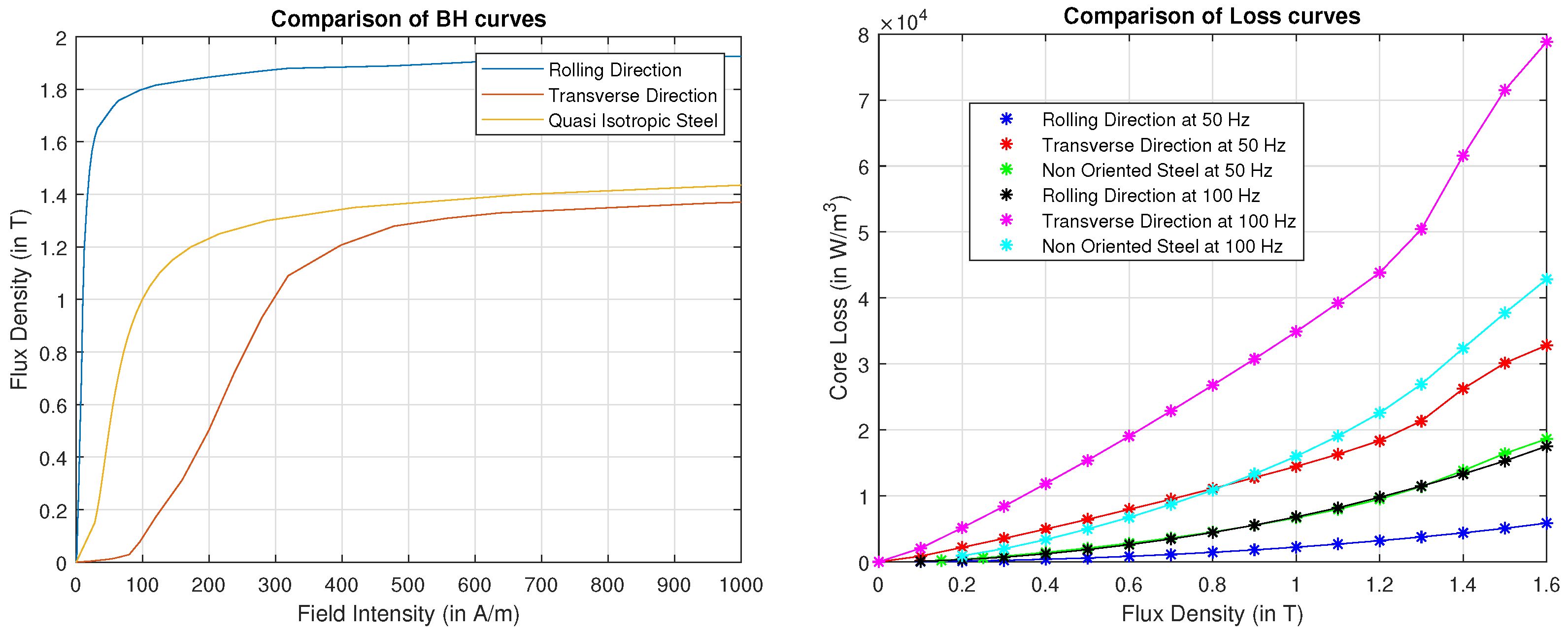
The performance of the anisotropic modular stator PMSM is compared with modular and non-modular non-oriented steel PMSMs. The BH and loss curves in oriented and non-oriented steel are shown in Figure 15. The rolling direction has both higher permeability and lower losses compared to the non-oriented steel. Moreover, the non-oriented steel has slightly better permeability and lower losses compared to the transverse direction in the oriented steel. The design is analyzed using 4, 8, 9, 12, and 18 segments. The effect of the size of the parasitic gap is also considered. Laser-cutting tolerances result in a maximum possible parasitic gap of 0.2 mm. Therefore, in this study, the value of the parasitic air gap is increased from 0 mm, which is the ideal case, to 0.2 mm in steps of 0.05 mm. In this work, all the gaps are assumed to be uniform and equal between all the segments. The comparison of the three models—modular oriented steel stator ( A o r i ), modular non-oriented steel stator ( A n o n o r i ), and non-modular non-oriented steel stator ( A c o n v e n t i o n a l )—is discussed in the following sub sections.

5.1. Variation of λ d and λ q

In this section, a comparison of the average torque and core losses for A c o n v e n t i o n a l , A n o n o r i , and A o r i at point O, with the stator current = 100 A, the power angle = 120 , and speed = 1000 RPM, is presented.
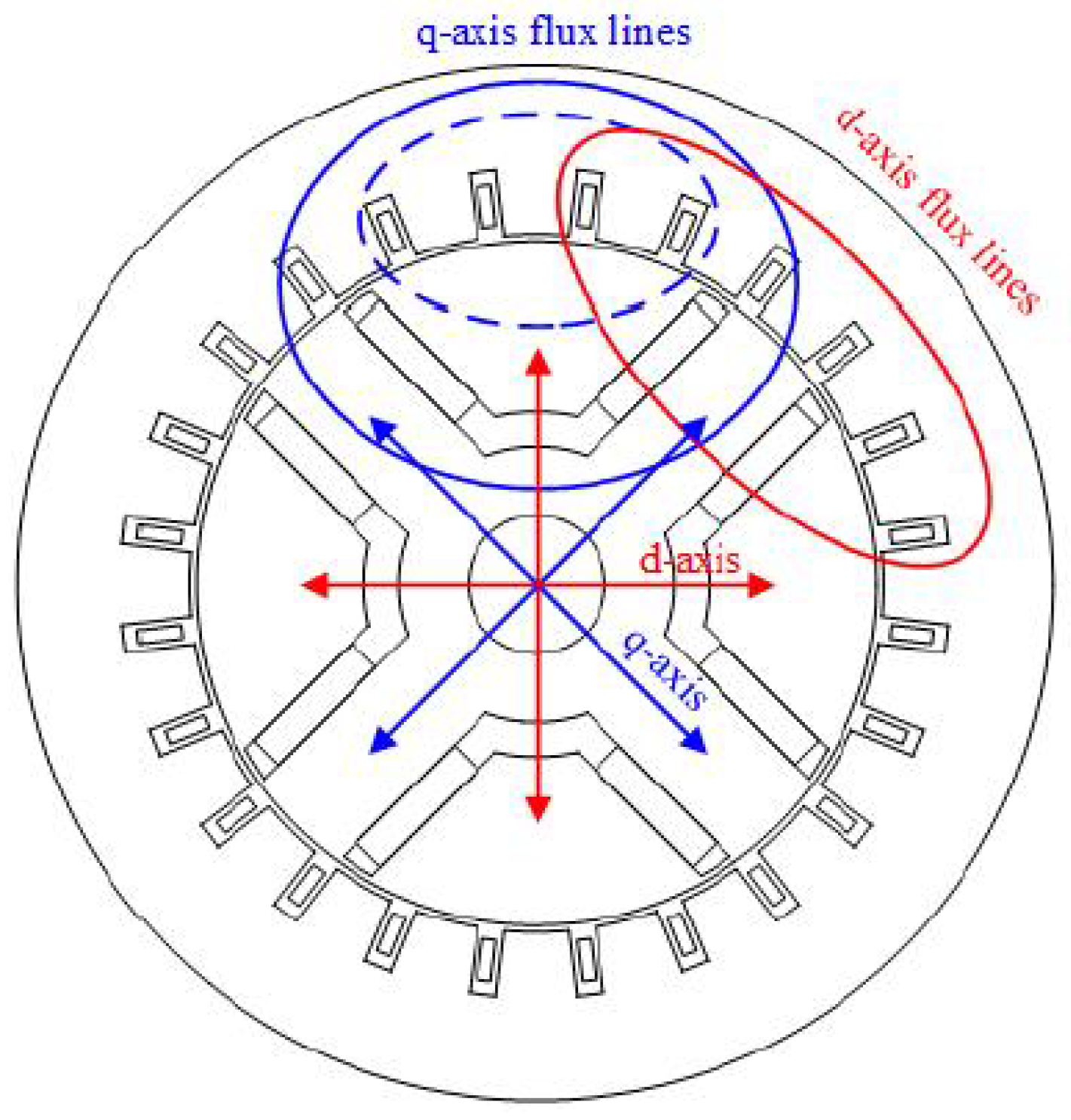
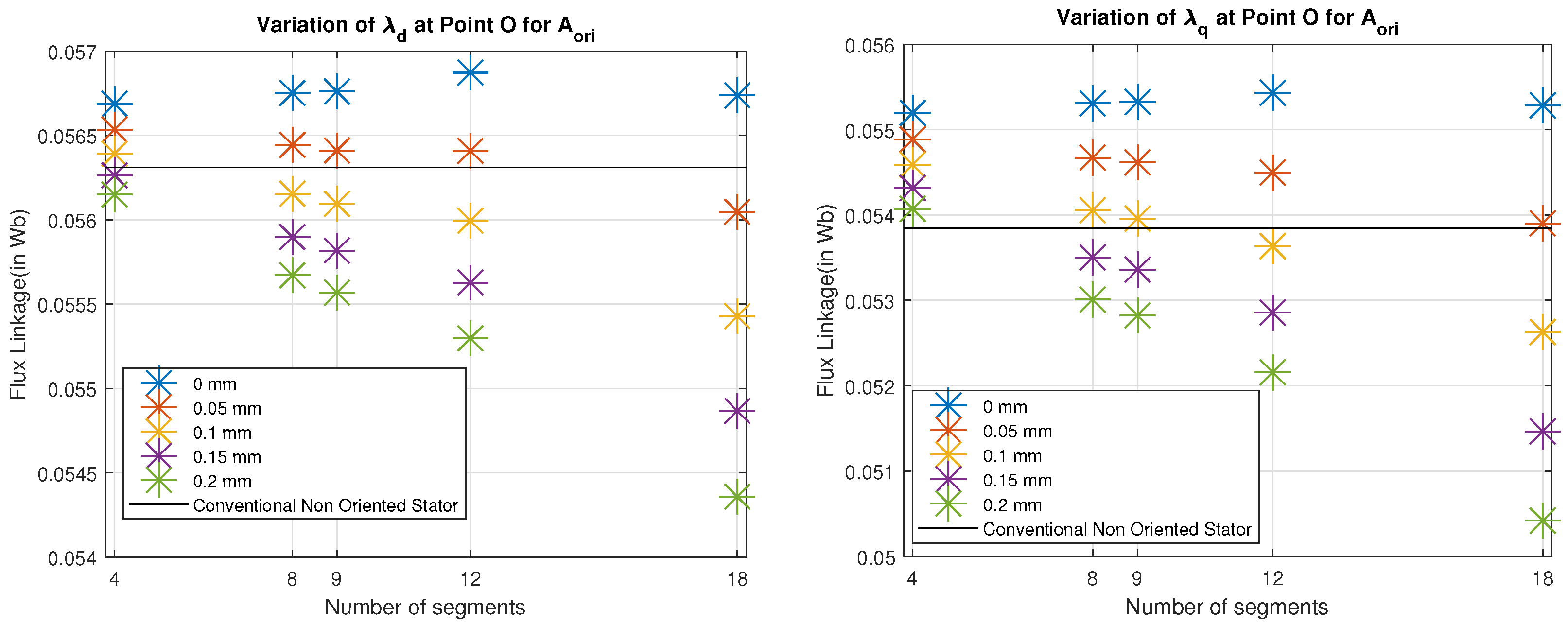
To explain the effect of oriented and non-oriented steel on core loss and average torque, the variation of the λ d and λ q linkage must be explained first. The values of λ d and λ q in the IPM are explained using the first reluctance path, the second reluctance path, and the magnet path, as proposed in [20] and shown in Figure 16. In [20], it is stated that the primary and secondary reluctance flux paths contribute towards λ q , while the magnet flux path contribute towards λ d . The presence of parasitic gaps between the segments in the stator leads to an increase in the reluctance in the direction of both the d- and q-axis flux paths. The reluctance in the d-axis flux path in the non-modular stator is due to the magnet, machine air gap, and steel present in both the stator and the rotor. On the other hand, the reluctance in the q-axis flux path in the non-modular stator is only due to the machine air gap and steel present in both stator and rotor. The reluctance of rare earth magnets is close to that of air. Therefore, segmentation leads to a higher change in the reluctance of the q-axis as compared to the d-axis, and also causes the decrease in the q-axis flux to be more dominant than the change in the d-axis flux. Moreover, the change in flux linkage due to the improved quality of steel is more prominent in the q-axis as compared to the d-axis. Figure 17 and Figure 18 show the variation of λ d and λ q at point O for A n o n o r i and A o r i , respectively, with the parasitic gaps and the number of segments supporting the claims made in this section.

5.2. Comparison of Core Loss

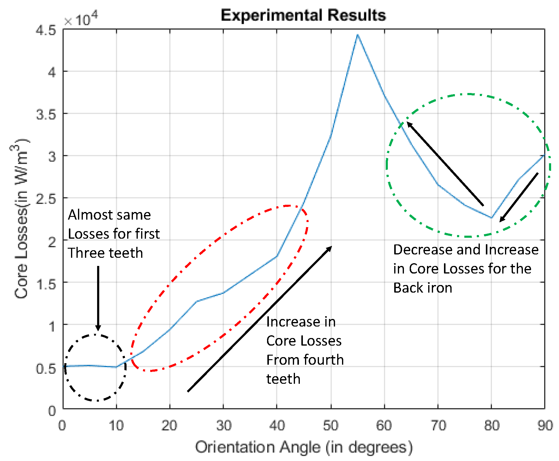
The three teeth closest to the rolling direction have almost identical magnetic properties, which are approximately the same as the properties in the rolling direction. There is an increase in the core losses from the fourth teeth onwards, i.e., more than 12 . 5 from the rolling direction, as shown in Figure 19.
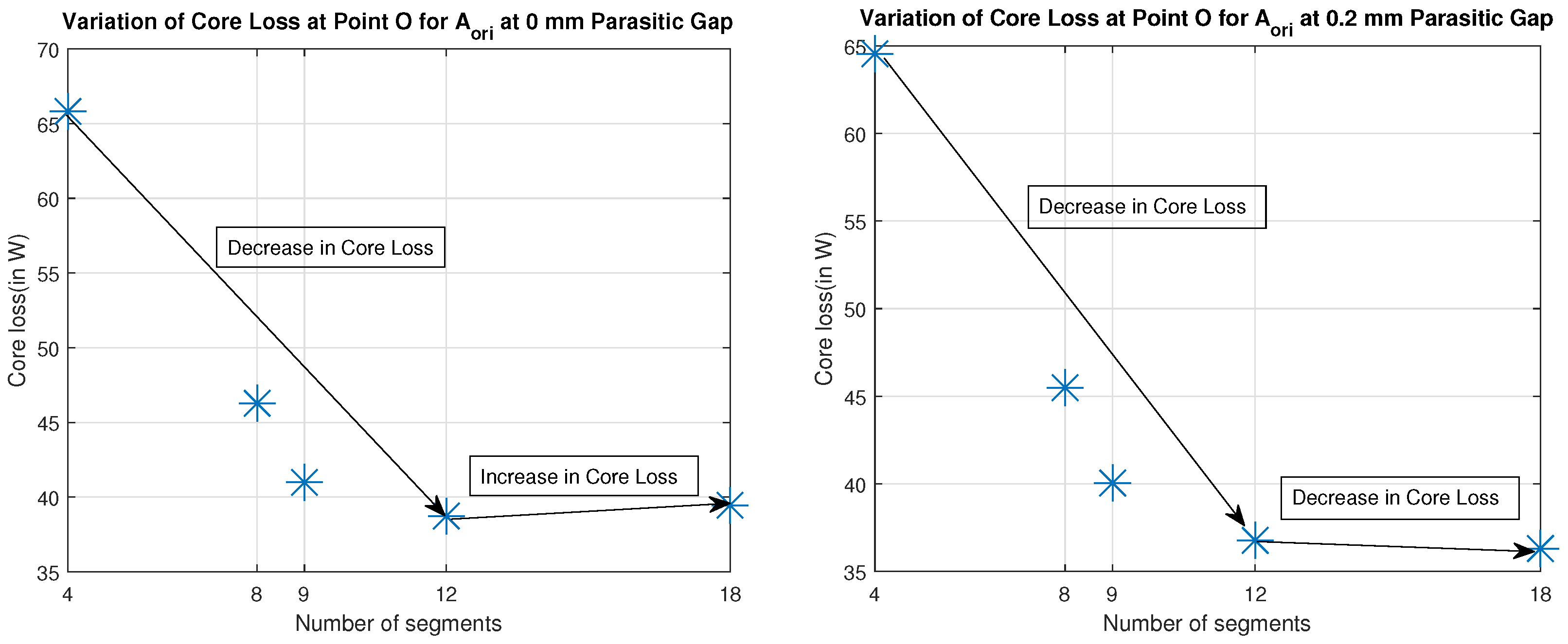
The core loss in the back iron decreases as the orientation angle changes from 90 to 80 , and then increases, as shown in Figure 19. This implies that the back iron has the best properties for the first three divisions. Therefore, when the number of teeth and back iron divisions are 6 in each segment, which means N s = 12 , the segment has the best possible magnetic properties when the value of the parasitic gap is 0 mm. However, the higher decrease in the flux linkage values for A o r i from N s = 12 to N s = 18 when the parasitic gap is 0.2 mm, shown in Figure 18, results in the decrease of the core loss from N s = 12 to N s = 18 . Figure 20 shows the variation of the core loss of the complete stator, with the number of segments for A o r i at point O for parasitic gap values of 0 mm and 0.2 mm.
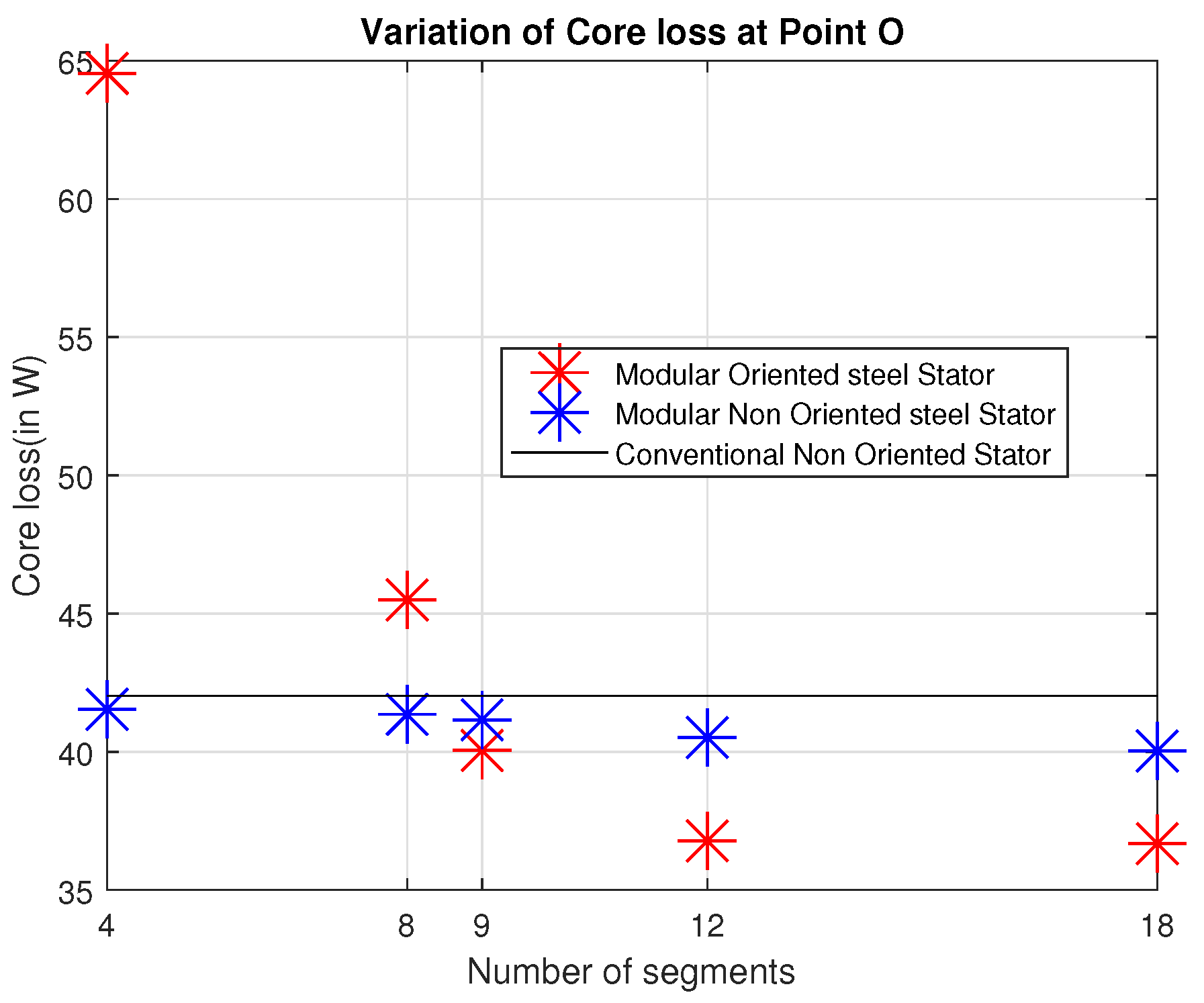
Moreover, due to the superior magnetic properties of the teeth of the A o r i , the losses are lower compared to the A n o n o r i and A c o n v e n t i o n a l when N s is 9, 12, and 18. The losses of A n o n o r i and A c o n v e n t i o n a l are almost similar due to same material being used in both machines. For the non-zero values of the parasitic gaps, the value of the core loss is lower for A n o n o r i than A c o n v e n t i o n a l due to the decrease in flux in the machine. Figure 21 shows the variation of the core loss, with the number of segments for all machines at point O, and a value of 0.2 mm for the parasitic gap.

5.3. Comparison of Average Torque

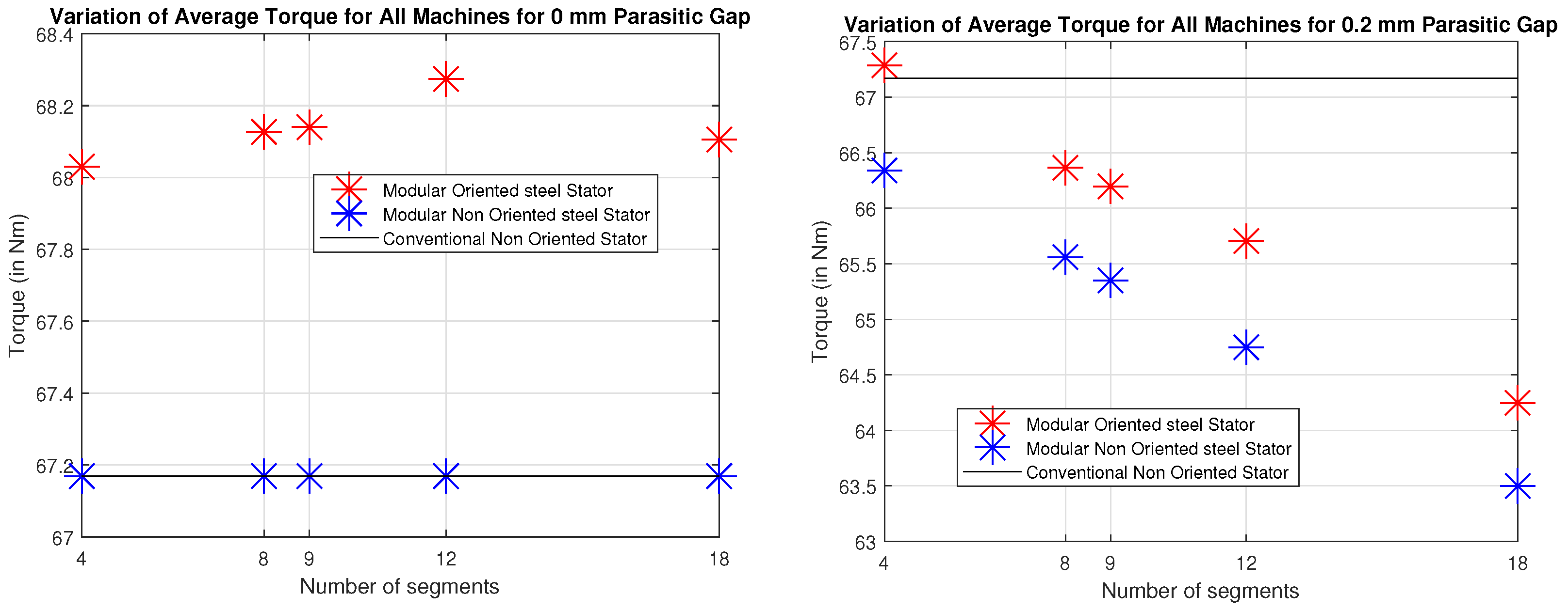
There is an improvement in the average torque in the A o r i compared with the A n o n o r i and A c o n v e n t i o n a l because of the higher permeability of the oriented steel when the value of the parasitic gaps between the segments is 0 mm. The value of the average torque is maximum when the number of segments is 12 for A o r i , as both λ d and λ q are maximized at N s = 12 for a 0 mm parasitic gap, as shown in Figure 18. However, when the parasitic gap is 0.2 mm, the values of both the d and q axis flux linkages are less as compared to the A c o n v e n t i o n a l machine, and hence the average torque is also lower. The only exception is when A o r i has four segments. As shown in Figure 18, the value of λ q is slightly higher for A o r i as compared to A c o n v e n t i o n a l when the parasitic gap is 0.2 mm, which overshadows the lower values of λ d , leading to a slightly higher torque for A o r i . Moreover, the average torque for A o r i is higher than A n o n o r i due to the better quality of the stator steel at all values of the parasitic gap, with same value of N s . Finally, the average torque value for A n o n o r i is lower compared to the A c o n v e n t i o n a l due to the decrease in flux linkage when the values of the parasitic gaps are non-zero. Figure 22 shows the variation of the average torque, with the number of segments for all machines and for parasitic gap values of 0 and 0.2 mm.

6. Selection of the Number of Segments for the Best Possible Performance of the Machine

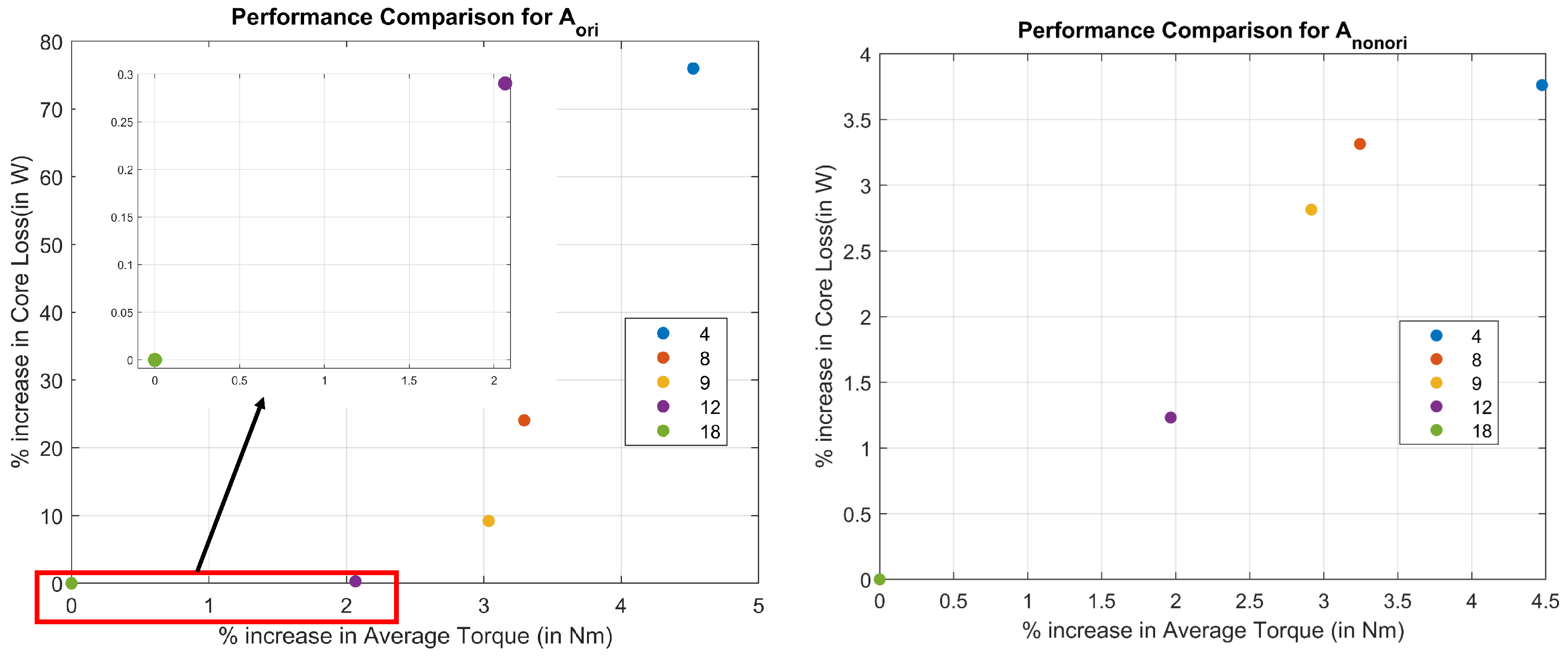
The selection criterion considers the worst possible scenario, i.e., when the parasitic gaps between the segments is 0.2 mm. Figure 23 shows the % change in the values of average torque and core loss from the reference value of N s = 18 , which shows the minimum average torque and the minimum core losses at point O.
  • Selection of Number of Segments for the Oriented Steel Model
    First, it is clear from Figure 23 that the increase in average torque is much less than the increase in core loss as the number of segments is decreased from 18 to 4. Second, the increase in core loss from N s = 18 to N s = 12 is negligibly small; however, there is a significant increase in the average torque. Third, for 8, 9, and 4 segments, there is an increase in the average torque as compared to N s = 12 . However, the increase in core loss is far greater than the increase in the average torque. The value of the lower torque for N s = 12 can be compensated by injecting a slightly higher current, which will lead to slightly higher core and copper losses. An analysis of the machine with an increased current is part of future work, and beyond the scope of this paper. Nevertheless, considering the two objectives of average torque and core losses, it can be inferred that for A o r i , the best possible performance is obtained from a machine consisting of 12 segments.
  • Selection of Number of Segments for the Non-Oriented Model
    Figure 23 shows the almost-linear trend of the increase in core losses and average torque for the A n o n o r i machine, from N s = 18 to N s = 4 . This is due to the fact that as the number of segments decreases, the flux in the machine increases, which then leads to a decrease in both core loss and average torque. Similar to the A o r i case, the lost torque can be increased by injecting slightly more current. Only an analysis that considers both core loss and copper loss at higher values of current for same torque can provide details for the best possible selection of the number of segments for A n o n o r i .

7. Conclusions

In this paper, a method for estimating the magnetic characteristics of oriented steel was proposed. The method utilized oriented steel segments and flux-injecting probes to obtain the magnetic characteristics of the oriented steel. This data were then used to model a modular stator consisting of oriented steel. It was shown that the experimentally-extracted magnetic characteristics of the oriented steel were different from the FEA method that utilized the properties of both the rolling and transverse directions to interpolate the magnetic characteristics. The obtained magnetic characteristics of the oriented steel were used to model the modular machine, and the oriented steel modular stator was compared to the non-oriented modular and non-modular stators.
The analysis showed that the number of segments in the oriented-steel modular-stator machine can be selected to minimize losses, although this selection is likely design-specific. For example, this was 12 segments for the unloaded machine and 18 segments for the loaded machine. Additionally, for the sample machine, the oriented steel modular stator machine had less loss for all values of the segments as compared to the non-modular and modular non-oriented steel machines under loaded and unloaded conditions. An improvement in the values of the average torque was also shown for the oriented steel modular stator machine as compared to the non-modular and modular non-oriented stator machines. However, the improvement was overshadowed at higher values of the number of segments due to the presence of parasitic gaps. The only exception to this variation was the improvement of the average torque for the oriented-steel machine with four segments. Moreover, the average torque of the non-oriented modular stator machine was lower compared to the non-modular non-oriented steel machine due to the presence of the parasitic gaps. Finally, it was shown that the oriented steel machine performs best when the number of segments is 12, while taking into account both objectives: core losses and average torque.
Future work should include an analysis of the oriented steel modular stator and the homogeneous steel modular stator machines at slightly higher currents in order to compare the core losses and copper losses for the same average torque. Finally, the stator will be redesigned for the oriented modular stator machine to achieve the desired objectives of core loss minimization and average torque maximization.

Author Contributions

Conceptualization, A.A.; methodology, A.A.; software, A.A.; validation, A.A.; formal analysis, A.A.; investigation, A.A.; resources, A.A.; data curation, A.A.; writing—original draft preparation, A.A. and M.M.; writing—review and editing, A.A., M.M., E.S. and J.A.; visualization, A.A.; supervision, E.S.; project administration, J.A.; funding acquisition, J.A. All authors have read and agreed to the published version of the manuscript.

Funding

This research was funded by GM Global Technical Center, Warren, MI, USA grant number GAC 3146.

Institutional Review Board Statement

Not applicable.

Informed Consent Statement

Informed consent was obtained from all subjects involved in the study.

Conflicts of Interest

The authors declare no conflict of interest.

References

  1. Li, G.J.; Zhu, Z.Q.; Foster, M.; Stone, D. Comparative Studies of Modular and Unequal Tooth PM Machines Either With or Without Tooth Tips. IEEE Trans. Magn. 2014, 50, 1–10. [Google Scholar] [CrossRef]
  2. Aggarwal, A.; Strangas, E.G.; Karlis, A. Review of Segmented Stator and Rotor Designs for AC Electric Machines. In Proceedings of the 2020 International Conference on Electrical Machines (ICEM), Gothenburg, Sweden, 23–26 August 2020; pp. 2342–2348. [Google Scholar]
  3. Huang, S.; Strangas, E.G.; Aggarwal, A.; Li, K.; Niu, F. Robust Inter-turn Short-circuit Detection in PMSMs with Respect to Current Controller Bandwidth. In Proceedings of the 2019 IEEE Energy Conversion Congress and Exposition (ECCE), Baltimore, MD, USA, 29 September–3 October 2019; pp. 3897–3904. [Google Scholar]
  4. Huang, S.; Aggarwal, A.; Strangas, E.G.; Li, K.; Niu, F.; Huang, X. Robust Stator Winding Fault Detection in PMSMs With Respect to Current Controller Bandwidth. IEEE Trans. Power Electron. 2021, 36, 5032–5042. [Google Scholar] [CrossRef]
  5. Aggarwal, A.; Strangas, E.G.; Agapiou, J. Robust Voltage based Technique for Automatic Off-Line Detection of Static Eccentricity of PMSM. In Proceedings of the 2019 IEEE International Electric Machines Drives Conference (IEMDC), San Diego, CA, USA, 12–15 May 2019; pp. 351–358. [Google Scholar]
  6. Aggarwal, A.; Allafi, I.M.; Strangas, E.G.; Agapiou, J.S. Off-Line Detection of Static Eccentricity of PMSM Robust to Machine Operating Temperature and Rotor Position Misalignment Using Incremental Inductance Approach. IEEE Trans. Transp. Electrif. 2021, 7, 161–169. [Google Scholar] [CrossRef]
  7. Aggarwal, A.; Strangas, E.G. Review of Detection Methods of Static Eccentricity for Interior Permanent Magnet Synchronous Machine. Energies 2019, 12, 4105. [Google Scholar] [CrossRef] [Green Version]
  8. Li, G.J.; Zhu, Z.Q.; Foster, M.P.; Stone, D.A.; Zhan, H.L. Modular Permanent-Magnet Machines With Alternate Teeth Having Tooth Tips. IEEE Trans. Ind. Electron. 2015, 62, 6120–6130. [Google Scholar] [CrossRef] [Green Version]
  9. Tomida, T.; Sano, N.; Hinotani, S.; Fujiwara, K.; Kotera, H.; Nishiyama, N.; Ikkai, Y. Application of fine-grained doubly oriented electrical steel to IPM synchronous motor. IEEE Trans. Magn. 2005, 41, 4063–4065. [Google Scholar] [CrossRef]
  10. Sugawara, Y.; Akatsu, K. Characteristics of a Switched Reluctance Motor using Grain-Oriented electric steel sheet. In Proceedings of the 2013 International Conference on Electrical Machines and Systems (ICEMS), Busan, Korea, 26–29 October 2013; pp. 18–23. [Google Scholar] [CrossRef]
  11. Ma, J.; Li, J.; Fang, H.; Li, Z.; Liang, Z.; Fu, Z.; Xiao, L.; Qu, R. Optimal Design of an Axial-Flux Switched Reluctance Motor With Grain-Oriented Electrical Steel. IEEE Trans. Ind. Appl. 2017, 53, 5327–5337. [Google Scholar] [CrossRef]
  12. Chwastek, K.R.; Baghel, A.P.S.; de Campos, M.F.; Kulkarni, S.V.; Szczygłowski, J. A Description for the Anisotropy of Magnetic Properties of Grain-Oriented Steels. IEEE Trans. Magn. 2015, 51, 1–5. [Google Scholar] [CrossRef]
  13. Liu, J.; Basak, A.; Moses, A.; Shirkoohi, G. A method of anisotropic steel modelling using finite element method with confirmation by experimental results. IEEE Trans. Magn. 1994, 30, 3391–3394. [Google Scholar] [CrossRef]
  14. Lin, D.; Zhou, P.; Badics, Z.; Fu, W.; Chen, Q.; Cendes, Z. A new nonlinear anisotropic model for soft magnetic materials. IEEE Trans. Magn. 2006, 42, 963–966. [Google Scholar] [CrossRef]
  15. Di Napoli, A.; Paggi, R. A model of anisotropic grain-oriented steel. IEEE Trans. Magn. 1983, 19, 1557–1561. [Google Scholar] [CrossRef]
  16. Gao, L.; Zeng, L.; Yang, J.; Pei, R. Application of grain-oriented electrical steel used in super-high speed electric machines. AIP Adv. 2020, 10, 015127. [Google Scholar] [CrossRef]
  17. Maraví-Nieto, J.; Azar, Z.; Thomas, A.; Zhu, Z. Utilisation of grain-oriented electrical steel in permanent magnet fractional-slot modular machines. J. Eng. 2019, 2019, 3682–3686. [Google Scholar] [CrossRef]
  18. Nazrulla, S.; Strangas, E.G.; Agapiou, J.S.; Perry, T.A. A Device for the Study of Electrical Steel Losses in Stator Lamination Stacks. IEEE Trans. Ind. Electron. 2014, 61, 2217–2224. [Google Scholar] [CrossRef]
  19. Jeong, K.; Ren, Z.; Yoon, H.; Koh, C. Measurement of Stator Core Loss of an Induction Motor at Each Manufacturing Process. J. Electr. Eng. Technol. 2014, 9, 1309–1314. [Google Scholar] [CrossRef] [Green Version]
  20. Hayslett, S.; Strangas, E. Analytical Design of Sculpted Rotor Interior Permanent Magnet Machines. Energies 2021, 14, 5109. [Google Scholar] [CrossRef]
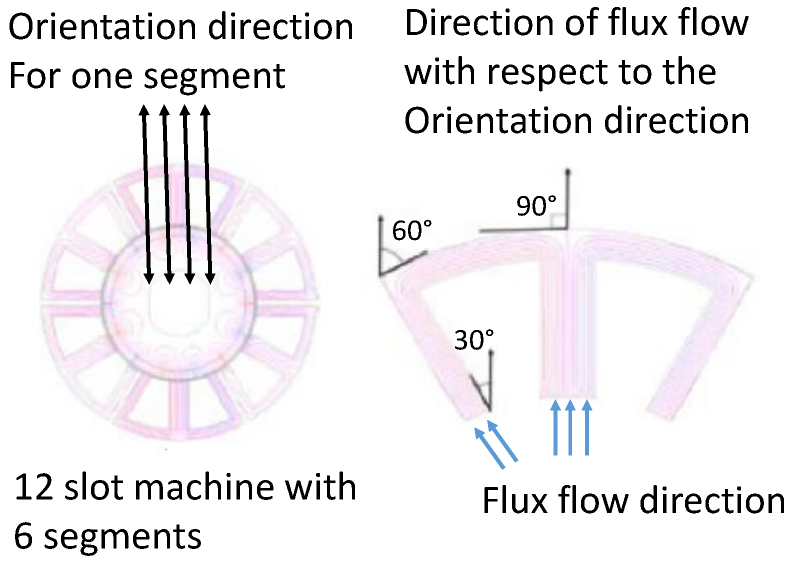
Figure 1. Direction of orientation and flux flow in the whole machine and in one segment [17].
Energies 14 06583 g001
Figure 2. One of the segments of the piecewise isotropic model used for analysis of the 12-slot machine consisting of six segments. Each colour corresponds with the angle away from the rolling direction that uses the magnetic properties of the oriented steel for that angle [17].
Energies 14 06583 g002
Figure 3. An example of a 72-tooth machine with 4 and 6 segments showing which teeth and back iron sections have similar magnetic properties.
Energies 14 06583 g003
Figure 4. Experimental set-up consisting of oriented steel segments, a sensor, a drive coil, and a pick-up coil.
Energies 14 06583 g004
Figure 5. Conceptual drawing of the flux lines in the portion of the segment injected by the sensor spanning over one tooth.
Energies 14 06583 g005
Figure 6. An example showing the line of symmetry that divides the segment into two identical halves.
Energies 14 06583 g006
Figure 7. Symmetry of the back iron sections of one segment for a 72-tooth machine consisting of four segments.
Energies 14 06583 g007
Figure 8. The division of one segment showing the relative placement of the teeth for a machine consisting of 72 teeth and four segments based on symmetry.
Energies 14 06583 g008
Figure 9. Positioning of Sensor A in positions A 1 and A 2 .
Energies 14 06583 g009
Figure 10. Sensor characterization experimental set-up with small steel pieces for all sensors.
Energies 14 06583 g010
Figure 11. Experimental set-up consisting of a sensor and a stator with the drive, pick-up, and control coils.
Energies 14 06583 g011
Figure 12. Schematics showing the overall experimental set-up and its main components.
Energies 14 06583 g012
Figure 13. Comparison of the core losses obtained from the analysis of experimental results and the FEA-interpolated core loss curves using the built-in function in the JMAG software for different angles away from the rolling direction, at a supply frequency of 50 Hz.
Energies 14 06583 g013
Figure 14. The variation of core losses, with an orientation angle obtained from the analysis of experimental results and simulations using the JMAG FEA software at 1.5 T and a supply frequency of 50 Hz.
Energies 14 06583 g014
Figure 15. Comparison of the BH and core loss curves for the rolling, transverse direction and the quasi-isotropic steel.
Energies 14 06583 g015
Figure 16. IPM flux paths: first reluctance path (solid blue), second reluctance path (dashed blue), and magnet path (solid red) [20].
Energies 14 06583 g016
Figure 17. Variation of λ d and λ q for A n o n o r i at I s = 100 A, δ = 120 , and speed = 1000 RPM.
Energies 14 06583 g017
Figure 18. Variation of λ d and λ q for A o r i at I s = 100 A, δ = 120 , and speed = 1000 RPM.
Energies 14 06583 g018
Figure 19. The variation of core losses with the orientation angle obtained from the analysis of experimental results, at 1.5 T and a supply frequency of 50 Hz. This shows the core loss variation for the teeth and the back iron from the line of symmetry.
Energies 14 06583 g019
Figure 20. Core loss variation of the complete stator for A o r i at I s = 100 A, δ = 120 , and speed = 1000 RPM at a parasitic gap of 0 mm and 0.2 mm.
Energies 14 06583 g020
Figure 21. Core loss variation for all machines at I s = 100 A, δ = 120 , and speed = 1000 RPM, and a parasitic gap value of 0.2 mm.
Energies 14 06583 g021
Figure 22. Variation of average torque with the number of segments for all machines and parasitic gaps of 0 and 0.2 mm.
Energies 14 06583 g022
Figure 23. Comparison of the performance of different numbers of segments for oriented and non-oriented segmented stators at I s = 100 A, δ = 120 , and speed = 1000 RPM, with a parasitic gap value of 0.2 mm.
Energies 14 06583 g023
Table 1. Values of B ^ l i m b and the frequency used to perform the experiments.
Supply Frequency (in Hz)Levels of B ^ limb (in T)
500.2, 0.4, 0.6, 0.8, 1.0, 1.2, 1.4, 1.5
1000.2, 0.4, 0.6, 0.8, 1.0, 1.2, 1.4
1500.2, 0.4, 0.6, 0.8, 1.0, 1.2, 1.3
Publisher’s Note: MDPI stays neutral with regard to jurisdictional claims in published maps and institutional affiliations.