The Multi-Advective Water Mixing Approach for Transport through Heterogeneous Media

Abstract

Finding a numerical method to model solute transport in porous media with high heterogeneity is crucial, especially when chemical reactions are involved. The phase space formulation termed the multi-advective water mixing approach (MAWMA) was proposed to address this issue. The water parcel method (WP) may be obtained by discretizing MAWMA in space, time, and velocity. WP needs two transition matrices of velocity to reproduce advection (Markovian in space) and mixing (Markovian in time), separately. The matrices express the transition probability of water instead of individual solute concentration. This entails a change in concept, since the entire transport phenomenon is defined by the water phase. Concentration is reduced to a chemical attribute. The water transition matrix is obtained and is demonstrated to be constant in time. Moreover, the WP method is compared with the classic random walk method (RW) in a high heterogeneous domain. Results show that the WP adequately reproduces advection and dispersion, but overestimates mixing because mixing is a sub-velocity phase process. The WP method must, therefore, be extended to take into account incomplete mixing within velocity classes.

1. Introduction

The advection–dispersion equation (ADE) is the most widely used formulation to model solute transport through porous media. Yet, it does not adequately characterize transport in heterogeneous media [1,2,3] where dispersion grows with scale [4,5], non-equilibrium occurs [6,7], or breakthrough curves display tailing [8,9]. These features are not well represented by the ADE. Therefore, transport through heterogeneous media is called anomalous (i.e., non-Fickian transport). The problem becomes critical when chemical reactions are involved [10,11,12,13,14,15]. Anomalous transport can be observed at different scales: from pore [16,17,18], column [19,20] to field scale [21,22,23,24,25]. An alternative formulation for anomalous transport that takes advection, dispersion, and mixing into consideration is, therefore, warranted [26,27].

The structure of heterogeneity is usually well known at large (km) scales from geological understanding. Thus, below a certain scale, it is necessary to address the absence of structure definition. At this point, the velocity development shows Markovianity in space rather than time [28,29,30,31,32,33,34,35]. A number of alternatives to the ADE have been proposed to address anomalous transport. The most widely extended is the continuous time random walk (CTRW). It consists of random velocity transitions once the solute has travelled a certain space step. However, these transitions are not fully random processes, but correlated ones [36]. Thus, a transition matrix $M^{vs}$ is needed [18,37,38,39,40]. $M^{vs}$ stands for the matrix probability to change the velocity state v given a fixed space phase s step. In this context, velocity becomes a variable of concentration such as space and time. The solute dependency of velocity was expressed in a phase space formulation proposed by [41]. However, this formulation does not take into account mixing.

Mixing is a consequence of diffusion among water bodies at a given time. Therefore, mixing is Markovian in time in contrast to dispersion. This observation suggests that solute transport should be localized not only in space and time, but also in velocity. The localization in time is of paramount importance, since mixing has a direct impact on chemical reactions in fluids [42,43,44,45,46]. The classic definition of mixing is proportional to the concentration gradient [47]. In fast chemical reactions, the reaction rate may also be calculated with the concentration gradient [44]. However, [48] demonstrated that mixing is due to the Brownian movement of single particles. Although this is a downscaling formulation of [47] and leads to the same results, the comparison of these two expressions is inconsistent [49]. This inconsistency is evidenced by the fact that domains with constant concentration (where the concentration gradients are equal to zero) are defined as immobile zones by [47], even though they are full of diffusing solute particles. As an alternative, the water mixing approach (WMA) has recently been proposed [15,49]. WMA defines the mixing flux as an exchange of waters that carries the mean concentrations of the cells. Thus, mixing is dependent on the concentrations (i.e., number of particles that cross the cell interface) instead of on their gradients.

Dispersion and mixing are different processes, but they are closely linked [50,51]. Spreading is essentially driven by advection variability and tends to enhance the concentration contrast, which in turn enhances mixing [52,53,54,55]. The link is evidenced by the stretching and folding processes [56,57,58]. This link leads to a non-Fickian mixing at earlier times over a considerable period [2,31,32,36,59]. Fickian mixing at later times is attributed to the spreading rate [53].

Several formulations have been put forward to overcome the problems of the ADE [60]. At the continuum scale, alternative methods include CTRW [17,35,36,37,61,62,63,64,65,66,67], fractional derivatives in ADE [68,69], stochastic convective stream tube [70], or multi-rate mass transfer [10,71,72,73,74,75]. Given that chemical reaction occurs at pore scale [76], some pore-scale methods such as the lattice Boltzmann equation [77,78,79,80,81], smoothed particle hydrodynamics [14,82,83,84], pore network models [85,86,87,88,89,90,91], or density kernel methods [92,93] have been studied. Hybrid continuum–pore-scale methods have also been proposed [94,95,96]. All these approaches partially meet the requirements listed by [27].

Recently, the multi-advective water mixing approach (MAWMA) was advanced by [49,97] to simulate anomalous transport. MAWMA can be taken as a WMA extension. The MAWMA is a phase space formulation (detailed in Section 2) where velocity is a new dimension of the state variable. The anomalous nature of transport is addressed by acknowledging that concentrations will be variable, within a representative elementary volume, and that this variability correlates with velocity (e.g., concentration in an advancing front will tend to be larger in high velocity portions of the medium than in nearly stagnant portions). The water parcel method (WP) can be derived by discretizing space, time, and velocity (Section 3.1). The question is how to exchange solute mass among water parcels. Exchange will depend on the properties of the medium (notably hydraulic conductivity and porosity) and, especially, on heterogeneity. In this paper, we test the capacity of the WP model and the proposed mass exchange methods to reproduce transport through heterogeneous porous media.

2. Governing Equations

Soler-Sagarra et al. [97] proposed a phase space formulation (MAWMA) to describe solute transport through porous media while meeting the requirements of [27]. As a phase space formulation, MAWMA considers that concentration depends not only on space and time, but also on velocity, i.e., c = c(x,v,t) [M/L³]. Using velocity as a new dimension facilitates describing dispersion, because spreading results naturally from velocity variability, so that no explicit accounting is needed for dispersion. Advection and mixing processes are defined by fluxes f in both the space, $s$, and velocity, $v$, domains. That is,

$$\varphi \frac{\partial c\left(x,v,t\right)}{\partial t}=f_{adv,s}+f_{diff,s}+f_{adv,v}+f_{diff,v}+r$$

(1)

where $\varphi$ [L³/L³] is porosity, $t$ [T] is time, and r [M/L³/T] is a sink/source term, possibly reflecting chemical reactions. The first term on the right hand side (rhs) represents advection within a velocity class, traditionally expressed in terms of Darcy flux, which we prefer to write here as a function of velocity as q = $\varphi$v [L³/L²/T] (blue arrow in Figure 1) as follows

$$f_{adv,s}=-\varphi v\cdot \nabla c$$

(2)

The second term of the rhs represents diffusion within a velocity class, classically defined by Fick’s law (orange arrow in Figure 1). However, the water mixing approach (WMA) was proposed as an alternative by [15,49])

$$f_{diff,s}=-\nabla \cdot \left(\overline{q_{D}c}\right)$$

(3)

where the term $\overline{q_{D}c}$ is used to express solute exchanges associated to water mass exchanges, $q_D=\varphi D_w/L_D$ [L³/L²/T] is the water diffusion flux exchanged, $D_w$[L²/T] is the water molecular diffusion coefficient, and $L_D$ [L] is a characteristic diffusion scale. Equation (3) expresses diffusion as the exchange of water depending on the concentration instead of on its gradient.

The third term on the rhs of Equation (1) represents changes in c(x,v,t) due to changes in velocity (green arrow in Figure 1). [41]) expressed it in terms of solute mass probability p. We express it in terms of concentration considering that $p=\varphi c/M$ ($M$ being the total solute mass), which yields

$$f_{adv,v}=-\frac{v}{L_A}\varphi c+\underset{v^{\prime }}{\overset{}{{\displaystyle \int }}}{g}^{vs}\left(v|v^{\prime }\right)\frac{v}{L_A}\varphi c^{\prime }d{v}^{\prime }+r$$

(4)

where $L_A$ [L] is the characteristic advection length, $g^{vs}$ [TL⁻¹] is probability density of a velocity transition after covering a step $L_A$ in space, and c′ = c(x,v′,t). Note that the first term on the rhs of Equation (4) refers to transitions to velocity v. It does not involve any velocity integration because ${{\displaystyle \int }}_{v^{\prime }}^{}{g}^{vs}\left(v^{\prime }|v\right)d{v}^{\prime }=1$.

Finally, [49,97] proposed expressing diffusive transitions in velocity (purple arrow in Figure 1) as

$$f_{diff,v}={{\displaystyle \int }}_{v^{\prime }}^{}\varphi f^{vt}\left(v|v^{\prime }\right)c^{\prime }d{v}^{\prime }-{{\displaystyle \int }}_{v^{\prime }}^{}\varphi f^{vt}\left(v^{\prime }|v\right)cd{v}^{\prime }$$

(5)

where $f^{vt}$ [L⁻¹] is the probability density, per unit time, of diffusive transitions between velocity states v. The expression $\varphi f^{vt}$ has units of water flux.

Note that, as in WMA, all fluxes are expressed in terms of water instead of solute concentrations, which become a mere attribute of water. This is why we termed the formulation of Equation (4) multi-advective water mixing approach (MAWMA).

Equation (4) could also be expressed as a Lagrangian formulation. This requires revising the definition of a material derivative. D(·)/dt reflects all changes in a flowing element of water. Therefore, it is expressed as the partial derivative minus the changes in c caused by advection. Since we are defining $f_{adv,v}$ to represent advective velocity transitions, we can write the material derivative as

$$\varphi \frac{dc}{dt}=\varphi \frac{\partial c}{\partial t}+\varphi v\cdot \nabla c+\frac{v}{L_A}\varphi c-\underset{v^{\prime }}{\overset{}{{\displaystyle \int }}}{g}^{vs}\left(v|v^{\prime }\right)\frac{v}{L_A}\varphi c^{\prime }d{v}^{\prime }$$

(6)

This definition acknowledges that velocity transitions due to heterogeneity do not cause mixing, which helps us to focus on the impact of mixing, which depends exclusively on diffusive processes:

$$\varphi \frac{dc}{dt}=-\nabla \cdot \left(\overline{q_{D}c}\right)+{{\displaystyle \int }}_{v^{\prime }}^{}\varphi f^{vt}\left(v|v^{\prime }\right)c^{\prime }d{v}^{\prime }-{{\displaystyle \int }}_{v^{\prime }}^{}\varphi f^{vt}\left(v^{\prime }|v\right)cd{v}^{\prime }$$

(7)

3. Solution Method

The equation presented in the previous section can be solved with any numerical methods. Here, we present a modeling option (Section 3.1), termed the water parcel (WP) method, which is an extension of the one proposed by [49,97]. We present first this new extension, which require two transition probability matrices. We then describe the computation of these matrices and their properties.

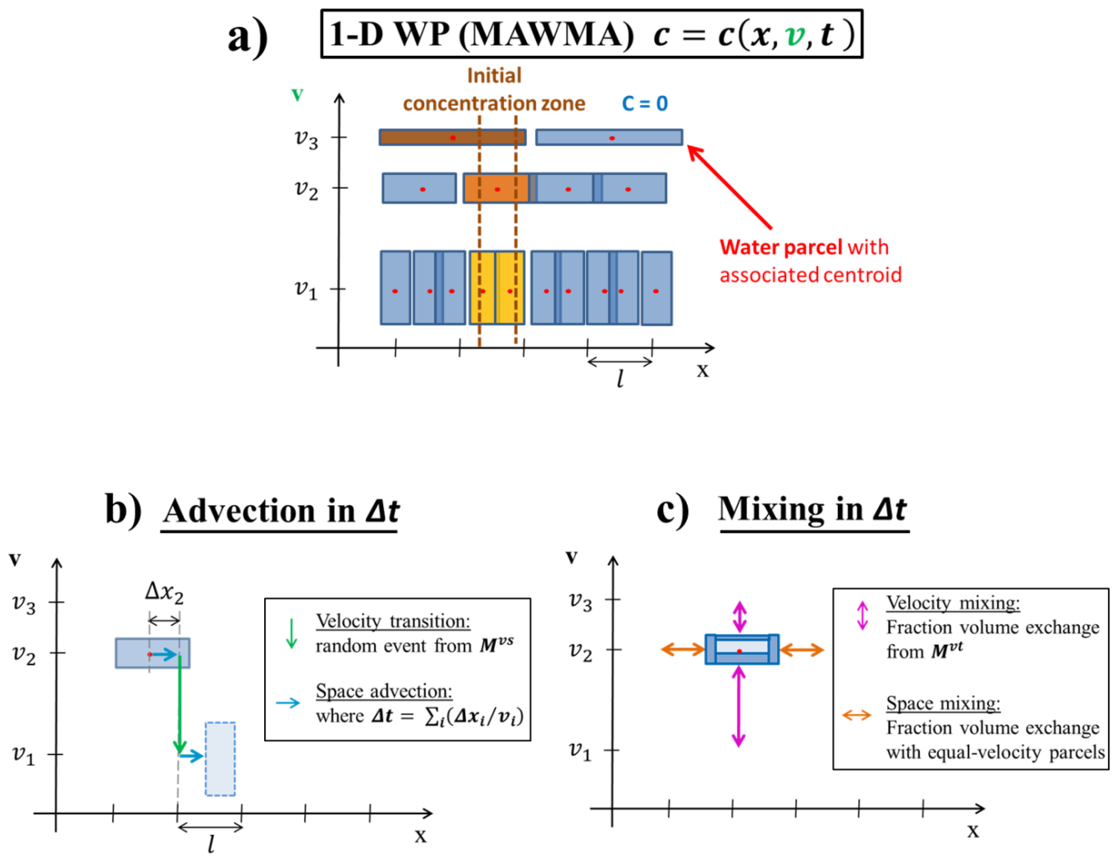
3.1. Water Parcel Method

Time, space, and velocity must be discretized to solve Equation (7). For simplicity, the discretization procedure is the one used by [49,97]. We reduce the spatial dimensions to 1 by integrating the dimensions perpendicular to the mean flow. The velocity field of the entire domain is discretized in classes with the same flux (i.e., equally probable in the Lagrangian velocity distribution). Since fast velocities concentrate most of the flux, they are less probable than slow velocities from an Eulerian point of view (they occupy less volume than slow velocities). Details of this velocity discretization are reported in [98]).

The space and velocity domains are discretized in parcels with the same water volume. Each water parcel is associated to its centroid, which determines the position (in space and velocity) at a given time. The length of a single parcel (i.e., its space extension along the x coordinate) is proportional to its velocity as reported by [15,49]. As a result, slow velocities have more parcels than fast velocities (see Figure 2a), which is consistent with their higher Eulerian probability (i.e., $p_e$ in [98]). The width is proportional to its probability (inversely proportional to its velocity). Equation (7) is integrated into the continuum space–velocity by using shape functions associated with each parcel. As in the finite volume method, the shape function equals 1 when (x,v) exists in the parcel domain. Otherwise, it equals to 0. Therefore, all attributes of water parcels (e.g., concentration) will be regarded as homogeneous within each parcel.

Parcels are injected and advected through the domain similar to solute particles. The injection velocity class is assigned randomly with equal probability for all classes to represent a uniform flux averaged injection.

Advection (Equations (2) and (4)) is simulated by simply displacing the parcel centroid with its associated velocity until it has covered the distance $L_A$. Then, a random event is performed to assign a new velocity for the next space step $L_A$ according to transition probabilities given by the transition matrix $M_{adv}^{vs}$ ($M_{ij}$ is the probability of jumping from velocity $v_j$ to $v_i$). This transition matrix is similar to the classic solute transition matrix $M^{vs}$ of [18,24,35,37,39,41] except that it only accounts for advection transitions. Since the simulation takes place with fixed time steps, each parcel will take a different number of steps to perform the next random event. The advection scheme is plotted in Figure 2b.

The discretized form of Equation (7) in a single parcel I of velocity class l is given by

$$V_w\frac{c_i^{k+1}-c_i^k}{\Delta t}={\displaystyle \sum }_{y\ne i}^{N_{li}}{F}_{iy}\left(c_y-c_i\right)+{\displaystyle \sum }_{m\ne l}^{N_v}{\displaystyle \sum }_j^{N_{mi}}{a}_{ij}{F}_{lm}^{vt}{c}_j^k-{\displaystyle \sum }_{m\ne l}^{N_v}{\displaystyle \sum }_j^{N_{mi}}{a}_{ji}{F}_{ml}^{vt}{c}_i^k i∊I_l$$

(8)

where V_w [L³] is the water volume of each parcel, $\Delta t$ [T] is the time step, N_li is the number of parcels $y$ with velocity l spatially connected to i, F is the water volumetric flux diffused, N_v is the number of velocity classes, N_mi is the number of parcels of velocity class m connected with parcel i, and $a_{ij}$ is the fraction of the diffusive flux assigned to velocity m, which will be exchanged with the j parcel. Recall that we interpret mixing as a water exchange process derived from water diffusion, which implies symmetry (i.e., $F_{iy}=F_{yi}$, $F_{lm}^{vt}=F_{ml}^{vt}$ and $a_{ij}=a_{ji}$) (the latter requires post processing).

We can rewrite Equation (8) using the concept of mixing ratio $\lambda =a \Delta t F/V_w$ [15], which leads to

$$c_i^{k+1}={\lambda }_{ii}{c}_i^k+{\displaystyle \sum }_{y\ne i}^{N_{li}}{\lambda }_{iy}^{}{c}_y^k+{\displaystyle \sum }_{m\ne l}^{N_v}{\displaystyle \sum }_j^{N_{mi}}{\lambda }_{ij}^{}{c}_j^k$$

(9)

The sum of all $\lambda$ equals 1, because the coefficients multiplying $c_j^k \left(\forall j\ne i\right)$ on the rhs of Equation (8) are always compensated by the same coefficient multiplying $-c_i^k$. Therefore, ${\lambda }_{ii}=1-{{\displaystyle \sum }}_y^{N_{li}}{\lambda }_{iy}-{{\displaystyle \sum }}_m^{N_v}{{\displaystyle \sum }}_j^{N_{mi}}{\lambda }_{ij}$. A necessary and sufficient condition for stability is that ${\lambda }_{ii}>0 \forall i$.

Equation (9) represents a mixing equation with mixing ratios that are independent of the species, which is consistent with the fact that it has been derived from the mixing of waters. Note that all transport processes described above involve water transfers. [15,49] explain the extension from Equation (9) to reactive transport.

3.2. Random Walk Method

The WP method described in Section 3.1 requires the velocity distribution, the diffusive transition matrix $M_{mix}^{vt}$ for mixing, and the advective transition matrix $M_{adv}^{vs}$. Here, we compute these from random walk simulations of flow and transport, which we will also use to test the proposed approach. The model to simulate flow is essentially that of [99]. We summarize it for the sake of completeness. A 2D multi-lognormal random permeability field $K\left(x\right)$ is generated with an isotropic Gaussian covariance function

$$\langle Y^{\prime }\left(x\right)Y^{\prime }\left(x^{\prime }\right)\rangle ={\sigma }_Y^{2}exp\left(-{\left(\frac{\left|x\right|}{L_A}\right)}^2\right)$$

(10)

where $Y^{\prime }\left(x\right)=Y\left(x\right)-Y\left(x\right)$, $Y\left(x\right)=ln\left(K\left(x\right)\right)$, and ${\sigma }_Y^2$ is the log-permeability variance. The random field $Y\left(x\right)$ with mean ${\mu }_Y=\langle Y\left(x\right)\rangle$ is generated using the Random Fields Package [100] of the R software environment [101]. Groundwater steady-state saturated flow is solved by imposing mass conservation and the Darcy equation:

$$v\left(x\right)=-\frac{K\left(x\right)\nabla h\left(x\right)}{\varphi }$$

(11)

where h is the hydraulic head. Fixed head boundary conditions are imposed to the upstream and downstream boundaries. No-flow conditions are imposed to the top and bottom boundaries. The flow model is solved by using the finite volume method to first obtain heads and, then, using Equation (11) for the velocity field $v\left(x\right)$.

A Python code is employed to solve particle transport. Particle advection is calculated as in [102]. Diffusion displacement at a given time step is $L_D$ξ, where ξ$~N\left(0,1\right)$.

3.3. Algebra of Mixing Matrices

The water mixing ratio ${\lambda }_{ij}$ defined in Section 3.1 can be understood as the $ij$-th position of the water transition matrix $M_{mix}^{vt}$ applied to time step. Here, we describe how to compute the mixing matrix $M_{mix}^{vt}$ from an RW simulation above the procedure as general, in the sense that it can be employed for advection transition matrices (applied after space steps) or mixing transition matrices (e.g., [15].

Transition matrices are obtained directly from their Markovian probability definition (i.e., $M_{ij}$ is the probability of a particle to end in velocity class $i$, given that it started in class$j$, which implicitly carries the Markovian statement that the next state solely depends on the current state). Therefore, $M_{ij}=N_{ij}^{k+1}/N_j^k$, where $N_{ij}^{k+1}$ is the number of particles that ended in velocity class $i$ at time $t^{k+1}$ after a diffusion step (to avoid advection transitions) having started in class$j$ at time $t^k$ and $N_j^k$. $M_{adv}^{vs}$ is computed analogously, except that accounting is made not at every time step, but after the particle has covered the characteristic advection scale.

Two issues need to be addressed. First, the above definition refers to probabilities, while we need volumetric water exchanges. Second, Markovianity needs to be tested. It was demonstrated by [35] for advection transitions, and it would be trivially true for mixing transitions in the absence of advection. However, it is not so clear when coupling advection and diffusion, especially when considering that low velocities occupy a much larger volume than high velocities. We will test Markovianity as part of the example in Section 4. However, we need first to clarify the relationship between transition probabilities and mixing matrices.

The relationship between the vector of solute probabilities p ($p_t$ according to [98]) and velocity class concentration is expressed as

$$p=m_T{}^{-1}Sc$$

(12)

where m_T is the total mass, and S is the storage matrix containing the volume of each class. S is not expressed in Eularian processes (time steps) as in Lagrangian processes (space steps). The procedure explained above to obtain the probability transition matrix M_p counting particle transitions in RW simulations can be expressed as

$$p^{k+1}=M_p{p}^k$$

(13)

Combining (12) and (13)

$$S{c}^{k+1}=M_{p}S{c}^k$$

(14)

Then, the concentrations for the next time step are as follows

$$c^{k+1}=S^{-1}{M}_{p}S{c}^k$$

(15)

Therefore, the transition matrix for transport simulations M_c can be obtained from the RW matrix M_p

$$M_c=S^{-1}{M}_{p}S$$

(16)

A well-known property of Markov probability transition matrices is that the sum of the columns of $M_p$ equals 1 (a particle in any velocity class must end in some class). However, the rows of the $M_c$ must add up to 1 to express that concentrations do not change if equal in all velocity classes. In fact, component $M_{Cij}$ can be viewed that as the volume of water received by class $i$ from class $j$, expressed as a fraction of the volume in $i$ (i.e., a mixing ratio), so that the rows must add up to 1 to also ensure that the class volume does not change. Therefore, the volume of water exchanged is expressed as

$$M_V=M_{p}S$$

(17)

To satisfy mass conservation, water volume exchanged between velocity classes i and j must be equal (i.e., $M_V$ must be symmetric). The computation procedure (starting with the probability transition matrix) does not ensure symmetry. In practice, it is nearly so. So, symmetry is imposed by setting

$$M_V=\frac{M_V^{\prime }{}^t+M_V^{\prime }}{2}$$

(18)

where $M_V^{\prime }$ is the volume exchange matrix computed initially from Equation (17). Finally, the water transition matrix is expressed as

$$M_w=S^{-1}{M}_V$$

(19)

While the properties of transition matrices are clear, and the equations in this section facilitate generalizing them for water parcels with varying volumes, which may be of interest for future applications, the question remains about the robustness of the proposed calculation method. Specifically, is it necessary to do a full RW simulation to compute the transition matrix?

4. Applications

Although WP is a continuum scale method, its solute evolution must reproduce the particle-based behavior [48]. This is why it is tested with the classic RW presented in Section 3.2. The model parameters are detailed in

Table 1. Flow and transport problem parameters and simulation details.

Flow		Transport
λ (m)	10	Num. time steps	100	$c_{ref}$ (kg/m3)	1
$L_x$	600λ	$\varphi$	0.3	Δt (s)	1
$L_y$	150λ	RW		Cases
Δx, Δy	λ/10	$N_{Particles}$	2.25 × 106	$D_w \left({\mathrm{m}}^2/\mathrm{s}\right)$	Peclet
${\mu }_Y^{}$	0	WP		0	$\infty$
${\sigma }_Y^2$	1	$N_v$	30	10−2	103
		$N_{parcels}$	1.44 × 105	0.2	50

. Three different Peclet number simulations are defined: $\infty$, 1000, and 50. The Peclet number is defined as follows

$$Pe=L_A\langle v\rangle /D_w$$

(20)

Initial concentrations are defined in both methods. The WP method employs the initial flux weighted distribution of solute mass (Figure 2a)

$$c_i\left(t=0\right)=c_{ref}\frac{v_i}{\langle v\rangle }$$

(21)

where $c_{ref}$ is the initial concentration reference, the angular bracket $\langle ·\rangle$ denotes the mean injection velocity (mean of the Lagrangian distribution), and $v_i$ is the parcel velocity.

In order to simulate a water parcel distribution, each particle of the RW method has an initial time step with a random definition Δt₀ = Δt·γ, being γ$~$unif(0,1). This definition provides an innovative way to simulate transport, since it differs from the classic Dirac delta. We believe it is a realistic situation, as it reproduces water injection. Other improvements from the classic RW method have been proposed [103]. Here, an initial number of particles $N_p$ are placed along the domain width $L_y$ at the fixed $x_0$ coordinate position. The particles have an initial flux-weighted distribution. This means that each cell in $x_0$ has $N_c$ particles, which is a function of the cell velocity $v_c$ expressed as follows

$$N_c=\frac{N_p}{L_y/\Delta y}\frac{v_c}{\langle v\rangle }$$

(22)

where Δy is the cell width. In order to simulate an injected concentration equal to 1, the mass of a single particle $m_p$ is

$$m_p=\frac{c_{ref}\varphi \langle v\rangle \Delta t{L}_y}{N_p}$$

(23)

The WP method should reproduce mean advection, dispersion, mixing, and “be flexible enough to be applicable to real problems” [27]. This latter condition is somewhat subjective and will not be considered here, but we believe that WP may be applied to field cases because (i) it is defined at the continuum scale, so that it can benefit from traditional hydrogeological characterization methods, (ii) it localizes concentration in the (x,v,t) continuum domain, and (iii) it is easily extended to reactive transport [15,49]. Still, a number of developments are needed to address the real cases with a level of maturity comparable to stochastic methods [32,104]. Therefore, we restrict ourselves to test advection, dispersion, and mixing on the synthetic case for stationary conditions and mean uniform flow. The spatial distribution of solute concentration for times 5, 20, and 100 s are shown in Figure 3.

The mean advection is characterized by the mean position$\mu$ defined as

$$\mu \left(t\right)=m_x^{\left(1\right)}\left(t\right)-x_0$$

(24)

where $m_x^{\left(k\right)}$ is the k-th order moment of the solute distribution in space

$$m_x^{\left(k\right)}\left(t\right)=\underset{\Omega }{\overset{}{{\displaystyle \int }}}c{x}^{k}d\Omega /\underset{\Omega }{\overset{}{{\displaystyle \int }}}cd\Omega$$

(25)

where $\Omega$ is the flow domain. From the above definition, we can express dispersion by the standard deviation of spatial solute distribution ${\sigma }_x^2$, which is described as

$${\sigma }_x^2\left(t\right)=m_x^{\left(2\right)}\left(t\right)-\mu {\left(t\right)}^2$$

(26)

Global mixing G [105] is defined as

$$G\left(t\right)=\underset{\Omega }{\overset{}{{\displaystyle \int }}}{c}^{2}d\Omega$$

(27)

Note that we can also define global mixing G′ in terms of the velocity domain such as

$$G^{\prime }\left(t\right)=\underset{v}{\overset{}{{\displaystyle \int }}}{c}^{\prime 2}dv$$

(28)

where c′ = c(v,t) is the mean concentration of an velocity class.

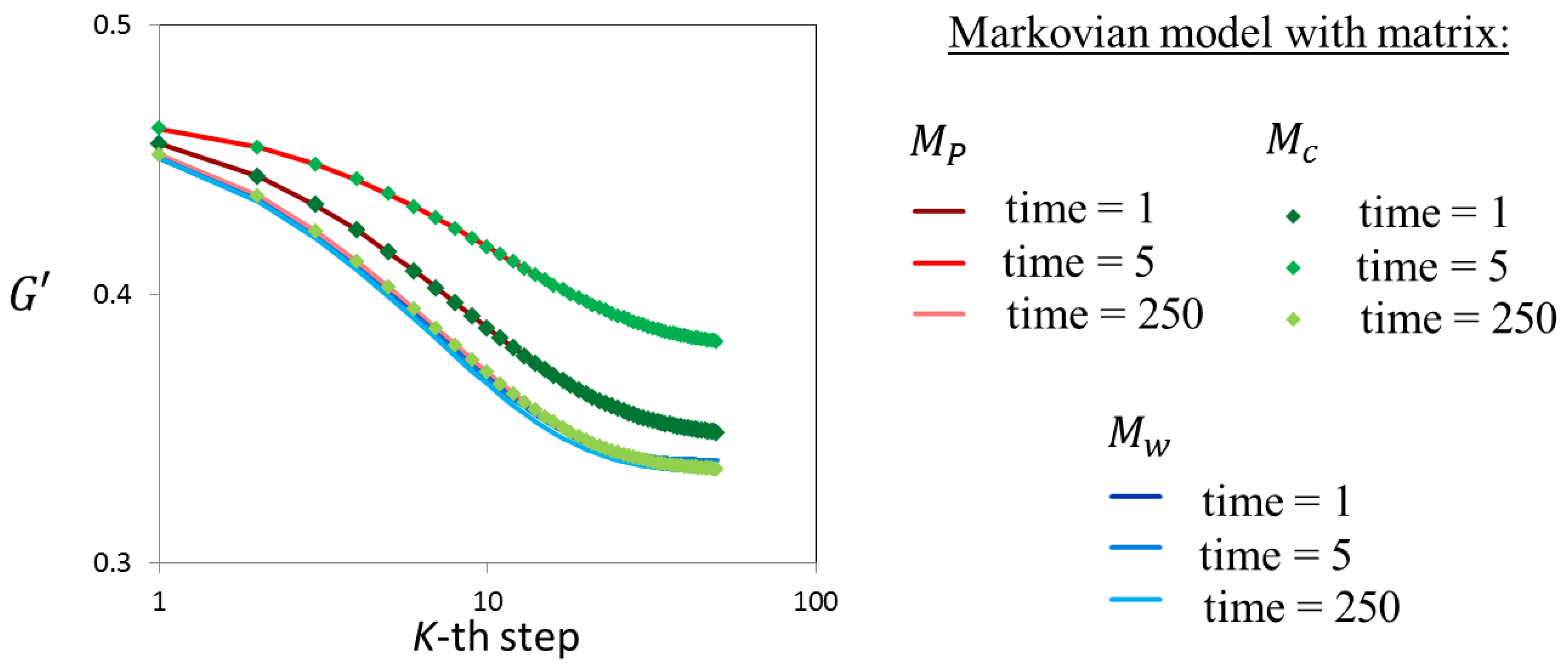
4.1. Transition Matrix Validation with Markovian Models

We defined three transition matrices in Section 3.3: $M_p$, $M_c$, and $M_w$. We test here the validity of their computation using a Markov chain model [106]. We first compute the probability transition matrix $M_p$ from RW (at ${\sigma }_Y^2=1$ and Pe = 50) simulations at three different times: t = 1, 5, and 250. The last time corresponds to the characteristic diffusive time (${\lambda }^2/2/D_w$), so that we can assume that injected particles have sampled exhaustively the whole velocity space (recall that we are using flux averaged injection, so that the slow velocities volume is less exhaustively sampled than the fast velocities volume).

Matrices $M_c$ and $M_w$ are calculated as explained in Section 3.3. Equation (13) defines the step computation for the matrices $M_p$. The Markovian models that employ M_c and M_w use concentration c instead of p as the state variable. Concentration c is readily converted to p by using (12). The initial solute probability distribution for any velocity class i is $p_i^0=1/N_v$.

The computed evolution of G′ (Equation (28)) in time is shown in Figure 4. The first observation from Figure 4 is that $\sigma$ decreases in time, which reflects that a uniform flow averaged probability leads to a non-uniform initial concentration. That is, the same mass flux occurs in all velocity classes, but concentration is much longer in the high velocity classes. Mixing causes the concentration to become uniform in all classes, so that G′ tends to decrease. Second, the M_p and M_c models evolve identically in time, although they are sensitive to the RW step in which they were computed. Third, we observe that the $M_w$ models always give identical results even though they are obtained from different $M_p$ matrices. The evolution computed with any of the $M_w$ matrices is identical to the one computed with the M_p and M_c matrices obtained after 250 RW steps. The evaluation method proposed for the $M_w$ matrix is indeed robust.

The mixing state decreases (higher G′ in Equation (28)) in the $M_p$ models from time t = 1 until reaching t = 5, when the poorest mixing state is attained. A state identical to $M_w$ is reached at the characteristic time of diffusion (t = 250), confirming that the water transitions are always constant. This occurs despite the heterogeneity of solute distributions within the velocity class and is of major significance because mixing can be defined in a constant water transition matrix during the entire simulation, which is not the case with the solute matrices.

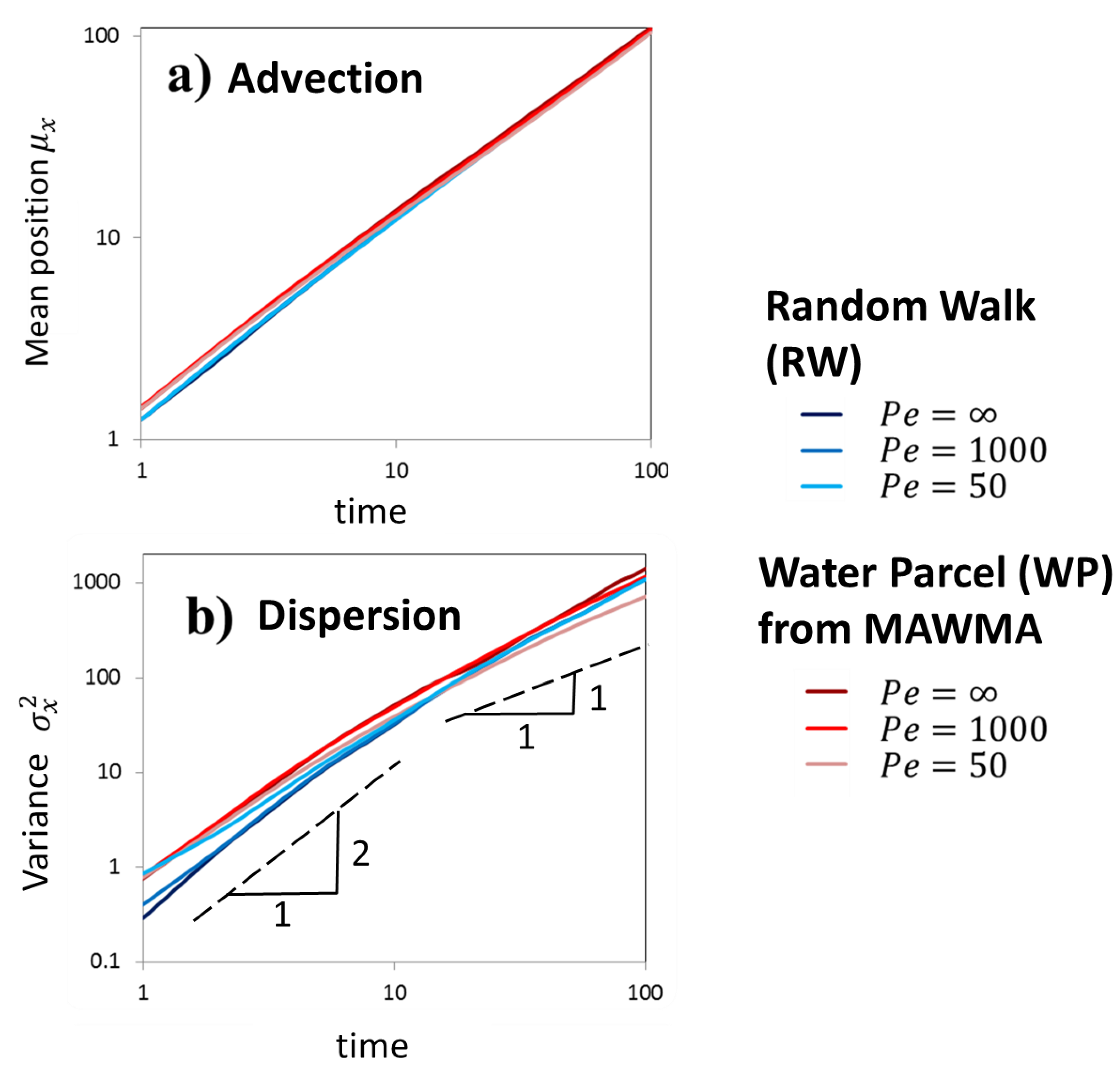
4.2. Comparison between RW and WP in Transport through Heterogeneous Porous Media

Mean position, spreading, and mixing results for MAWMA and RW and ${\sigma }_Y^2=1$ are shown in Figure 5 and Figure 6. A good fit of mean position $\mu$ (Equation (24)) can be observed for all cases in Figure 5a. Regarding spreading, the evolution of ${\sigma }_x^2$ (Equation (26)), using the RW, is consistent with those of [107,108] also showed that early time spreading of a Dirac Delta is controlled by velocity heterogeneities, thus becoming ballistic, so that the spatial variance is proportional to t². This explains differences in the $WP$ and $RW$ results in Figure 5b. The $WP$ grid is too coarse to reproduce early time advection of a Dirac pulse. This is not of great concern for practical applications, because this pulse initial condition is unusual in practice. The $RW$ and $WP$ results converge at later times, during the intermediate regime observed by [108] prior to the Fickian regime.

We compare the results of global mix G plotted in Figure 6. We first evaluate the $Pe=\infty$ case. The mismatch observed is due to the mesh evaluation. WP displays the correct constant G because the entire solute remains in the initial parcel. In other words, no mixing transition of solute occurs between parcels. By contrast, RW uses a structured mesh that is fixed for the evaluation of concentration. The number of concentrated elements increases with time due to stretching [109], which implies a reduction in the computed concentration; this is a common problem when comparing Eulerian (RW) and Lagrangian (WP) evaluations of concentration. For a more accurate comparison, RW should, therefore, be performed with a Lagrangian mesh (such as the one proposed by [15]).

In the other Pe cases, RW shows a monotonic decrease in G. However, WP underestimates mixing at early times. This mismatch is attributed to the mesh distinction given that similar discrepancies are again observed. In contrast, WP overestimates mixing with respect to RW at late times. This is consistent with the WP standard deviation behavior observed previously. We suspect this overestimation is related to incomplete mixing [110,111]. In other words, concentration variability remains at scales lower than velocity discretization, whereas WP changes the entire parcel concentration in the mixing process (i.e., homogenization), which confirms the mixing results observed in the above section. Some alternatives to incomplete mixing have been proposed [107]. However, the mixing criterion of these authors is dependent on the solute state, whereas we seek to base it on the water volumes.

5. Conclusions

We present and test the MAWMA formulation for transport through heterogeneous porous media using the WP solution method. The formulation is an extension of WMA, which considers transport of water instead of solute concentration. Exchange of water volumes is used to reproduce mixing instead of individual species diffusion. Individual species concentrations are considered attributes of water. They may vary spatially, in which case the net solute mass exchange turns out to be proportional to the concentration gradient. However, water and solutes exchanges occur independently of concentration gradients, which is why no concentration gradient is used to calculate the mixing process.

We use the WP method to reproduce MAWMA. WP requires a velocity discretization and two transition matrices: one to reproduce advection transitions, which is Markovian in space (i.e., transitions occur after fixed spatial steps, which is consistent with a fixed heterogeneity), and one to reproduce mixing, which is Markovian in time (i.e., velocity transitions occur at a constant rate in time, which is consistent with Brownian motion). We have described how to compute these matrices from RW models. Our study shows that it is possible to obtain the water transition matrices from the classic solute transition matrices.

We use Markovian models with transition matrices computed from different time steps of the RW simulations to compare transition matrices. We showed that, unlike M_c, M_w is invariant in time, and the proposed calculation method is robust. Then, we test the performance of WP of advection, dispersion, and mixing with the RW simulations. We find that advection (mean displacement) and dispersion (mean spreading) are similar for the two methods. However, mixing (2nd moment of concentration) results are different, which we attribute to two reasons: (a) mesh inequivalence and (b) incomplete mixing. The structured mesh of RW is Eulerian in contrast to the unstructured Lagrangian mesh used in WP. The WP method assumes a homogeneous concentration value within the parcel volume. However, in our study, this is inappropriate because the mixing scale (i.e., the scale at which concentration can be considered constant) is much smaller than the scale required for velocity definition.

In summary, the RW concentration evaluation requires a Lagrangian mesh (such as the isochronal one proposed by [15]). Moreover, WP needs a new evaluation of concentration in order to take into account heterogeneity inside the parcels. This new evaluation should consider water volumes, which will ensure the independence of concentration states. This will facilitate coupling with chemical reaction calculations.

References

1. Gjetvaj, F.; Russian, A.; Gouze, P.; Dentz, M. Dual control of flow field heterogeneity and immobile porosity on non-Fickian transport in Berea sandstone. Water Resour. Res. 2015, 51, 8273–8293. [Google Scholar] [CrossRef] [Green Version]
2. Le Borgne, T.; Gouze, P. Non-Fickian dispersion in porous media: 2. Model validation from measurements at different scales. Water Resour. Res. 2008, 44, 1–10. [Google Scholar] [CrossRef] [Green Version]
3. Willmann, M.; Carrera, J.; Sánchez-Vila, X. Transport upscaling in heterogeneous aquifers: What physical parameters control memory functions? Water Resour. Res. 2008, 44, 1–13. [Google Scholar] [CrossRef] [Green Version]
4. Gelhar, L.W.; Mantoglou, A.; Welty, C.; Rehfeldt, K.R. A Review of Field-Scale Physical Solute Transport Processes in Saturated and Unsaturated Porous Media. EPRI Report EA-4190. 1985. Available online: https://books.google.ro/books?id=iS33BwAAQBAJ&pg=PA296&lpg=PA296&dq=4.+Gelhar,+L.W.;+Mantoglou,+A.;+Welty,+C.;+Rehfeldt,+K.R.+A+Review+of+Field-Scale+Physical+Solute+Transport+Processes+in+Saturated+and+Unsaturated+Porous+Media;+EPRI+Report+EA-4190;+1985.&source=bl&ots=eQFqb2KYx6&sig=ACfU3U3Wm3zSPmLxECV8U0Q8szdKsqEppQ&hl=en&sa=X&ved=2ahUKEwim_b_S7sTzAhX2_7sIHUgkB-QQ6AF6BAgCEAM#v=onepage&q=4.%20Gelhar%2C%20L.W.%3B%20Mantoglou%2C%20A.%3B%20Welty%2C%20C.%3B%20Rehfeldt%2C%20K.R.%20A%20Review%20of%20Field-Scale%20Physical%20Solute%20Transport%20Processes%20in%20Saturated%20and%20Unsaturated%20Porous%20Media%3B%20EPRI%20Report%20EA-4190%3B%201985.&f=false (accessed on 15 September 2021).
5. Neuman, S.P. Universal scaling of hydraulic conductivities and dispersivities in geologic media. Water Resour. Res. 1990, 26, 1749–1758. [Google Scholar] [CrossRef]
6. Vogel, H.-J.; Cousin, I.; Ippisch, O.; Bastian, P. The dominant role of structure for solute transport in soil: Experimental evidence and modelling of structure and transport in a field experiment. Hydrol. Earth Syst. Sci. 2006, 10, 495–506. [Google Scholar] [CrossRef] [Green Version]
7. Alcolea, A.; Carrera, J.; Medina, A. Regularized pilot points method for reproducing the effect of small scale variability: Application to simulations of contaminant transport. J. Hydrol. 2008, 355, 76–90. [Google Scholar] [CrossRef]
8. Valocchi, A.J. Validity of the Local Equilibrium Assumption for Modeling Sorbing Solute Transport Through Homogeneous Soils. Water Resour. Res. 1985, 21, 808–820. [Google Scholar] [CrossRef]
9. Carrera, J. An overview of uncertainties in modelling groundwater solute transport. J. Contam. Hydrol. 1993, 13, 23–48. [Google Scholar] [CrossRef]
10. Soler-Sagarra, J.; Luquot, L.; Martínez-Pérez, L.; Saaltink, M.W.; De Gaspari, F.; Carrera, J. Simulation of chemical reaction localization using a multi-porosity reactive transport approach. Int. J. Greenh. Gas Control. 2016, 48, 59–68. [Google Scholar] [CrossRef]
11. Battiato, I.; Tartakovsky, D.; Scheibe, T. On breakdown of macroscopic models of mixing-controlled heterogeneous reactions in porous media. Adv. Water Resour. 2009, 32, 1664–1673. [Google Scholar] [CrossRef]
12. Sadhukhan, S.; Gouze, P.; Dutta, T. A simulation study of reactive flow in 2-D involving dissolution and precipitation in sedimentary rocks. J. Hydrol. 2014, 519, 2101–2110. [Google Scholar] [CrossRef]
13. Scheibe, T.D.; Schuchardt, K.; Agarwal, K.; Chase, J.; Yang, X.; Palmer, B.J.; Tartakovsky, A.M.; Elsethagen, T.; Redden, G. Hybrid multiscale simulation of a mixing-controlled reaction. Adv. Water Resour. 2015, 83, 228–239. [Google Scholar] [CrossRef] [Green Version]
14. Tartakovsky, A.; Tartakovsky, G.; Scheibe, T. Effects of incomplete mixing on multicomponent reactive transport. Adv. Water Resour. 2009, 32, 1674–1679. [Google Scholar] [CrossRef]
15. Soler-Sagarra, J.; Saaltink, M.W.; Nardi, A.; De Gaspari, J.; Carrera, J. Water Mixing Approach (WMA) for Reactive Transport Modeling. 2021. submitted. Available online: http://blogs.uned.es/catedra-aquae/wp-content/uploads/sites/111/2021/06/Tesis-Joaquim-Soler.pdf (accessed on 15 September 2021).
16. Seymour, J.D.; Gage, J.P.; Codd, S.L.; Gerlach, R. Anomalous Fluid Transport in Porous Media Induced by Biofilm Growth. Phys. Rev. Lett. 2004, 93, 198103. [Google Scholar] [CrossRef] [PubMed]
17. Bijeljic, B.; Mostaghimi, P.; Blunt, M. Signature of Non-Fickian Solute Transport in Complex Heterogeneous Porous Media. Phys. Rev. Lett. 2011, 107, 204502. [Google Scholar] [CrossRef] [PubMed] [Green Version]
18. Kang, P.K.; de Anna, P.; Nunes, J.P.; Bijeljic, B.; Blunt, M.J.; Juanes, R. Pore-scale intermittent velocity structure underpinning anomalous transport through 3-D porous media. Geophys. Res. Lett. 2014, 41, 6184–6190. [Google Scholar] [CrossRef]
19. Hatano, Y.; Hatano, N. Dispersive transport of ions in column experiments: An explanation of long-tailed profiles. Water Resour. Res. 1998, 34, 1027–1033. [Google Scholar] [CrossRef]
20. Rinaldo, A.; Benettin, P.; Harman, C.J.; Hrachowitz, M.; McGuire, K.J.; van der Velde, Y.; Bertuzzo, E.; Botter, G. Solute transport in low-heterogeneity sandboxes: The role of correlation length and permeability variance. Water Resour. Res. 2015, 51, 4840–4847. [Google Scholar] [CrossRef] [Green Version]
21. Garabedian, S.P.; LeBlanc, D.R. Large-Scale natural gradient tracer test in sand and gravel, Cape Cod, Massachusetts 2. Analysis of spatial moments for a nonreactive tracer. Water Resour. Res. 1991, 27, 911–924. [Google Scholar] [CrossRef]
22. Becker, M.W.; Shapiro, A. Tracer transport in fractured crystalline rock: Evidence of nondiffusive breakthrough tailing. Water Resour. Res. 2000, 36, 1677–1686. [Google Scholar] [CrossRef] [Green Version]
23. McKenna, S.A.; Meigs, L.C.; Haggerty, R. Tracer tests in a fractured dolomite: 3. Double-porosity, multiple-rate mass transfer processes in convergent flow tracer tests. Water Resour. Res. 2001, 37, 1143–1154. [Google Scholar] [CrossRef] [Green Version]
24. Kang, P.K.; Le Borgne, T.; Dentz, M.; Bour, O.; Juanes, R. Impact of velocity correlation and distribution on transport in fractured media: Field evidence and theoretical model. Water Resour. Res. 2014, 51, 940–959. [Google Scholar] [CrossRef] [Green Version]
25. Zech, A.; Attinger, S.; Cvetkovic, V.; Dagan, G.; Dietrich, P.; Fiori, A.; Rubin, Y.; Teutsch, G. Is unique scaling of aquifer macrodispersivity supported by field data? Water Resour. Res. 2015, 51, 7662–7679. [Google Scholar] [CrossRef] [Green Version]
26. De Dreuzy, J.-R.; Carrera, J.; Dentz, M.; Le Borgne, T. Time evolution of mixing in heterogeneous porous media. Water Resour. Res. 2012, 48, W06511. [Google Scholar] [CrossRef] [Green Version]
27. De Dreuzy, J.-R.; Carrera, J. On the validity of effective formulations for transport through heterogeneous porous media. Hydrol. Earth Syst. Sci. 2016, 20, 1319–1330. [Google Scholar] [CrossRef] [Green Version]
28. Montroll, E.W.; Weiss, G.H. Random Walks on Lattices. II. J. Math. Phys. 1965, 6, 167–181. [Google Scholar] [CrossRef]
29. Scher, H.; Lax, M. Stochastic Transport in a Disordered Solid. I. Theory. Phys. Rev. B 1973, 7, 4491–4502. [Google Scholar] [CrossRef]
30. Metzler, R.; Klafter, J. The random walk’s guide to anomalous diffusion: A fractional dynamics approach. Phys. Rep. 2000, 339, 1–77. [Google Scholar] [CrossRef]
31. Berkowitz, B.; Cortis, A.; Dentz, M.; Scher, H. Modeling non-Fickian transport in geological formations as a continuous time random walk. Rev. Geophys. 2006, 44, 1–49. [Google Scholar] [CrossRef] [Green Version]
32. Neuman, S.P.; Tartakovsky, D.M. Perspective on theories of non-Fickian transport in heterogeneous media. Adv. Water Resour. 2009, 32, 670–680. [Google Scholar] [CrossRef]
33. Scher, H.; Montroll, E.W. Anomalous transit-time dispersion in amorphous solids. Phys. Rev. B 1975, 12, 2455–2477. [Google Scholar] [CrossRef]
34. Klafter, J.; Silbey, R. Derivation of the Continuous-Time Random-Walk Equation. Phys. Rev. Lett. 1980, 44, 55–58. [Google Scholar] [CrossRef] [Green Version]
35. Le Borgne, T.; Dentz, M.; Carrera, J. Spatial Markov processes for modeling Lagrangian particle dynamics in heterogeneous porous media. Phys. Rev. E 2008, 78, 026308. [Google Scholar] [CrossRef] [PubMed]
36. Le Borgne, T.; Dentz, M.; Carrera, J. Lagrangian Statistical Model for Transport in Highly Heterogeneous Velocity Fields. Phys. Rev. Lett. 2008, 101, 090601. [Google Scholar] [CrossRef] [PubMed] [Green Version]
37. Kang, P.; Dentz, M.; Le Borgne, T.; Juanes, R. Spatial Markov Model of Anomalous Transport Through Random Lattice Networks. Phys. Rev. Lett. 2011, 107, 180602. [Google Scholar] [CrossRef] [Green Version]
38. Benke, R.; Painter, S. Modeling conservative tracer transport in fracture networks with a hybrid approach based on the Boltzmann transport equation. Water Resour. Res. 2003, 39, 1–11. [Google Scholar] [CrossRef]
39. De Anna, P.; Le Borgne, T.; Dentz, M.; Tartakovsky, A.M.; Bolster, D.; Davy, P. Flow Intermittency, Dispersion, and Correlated Continuous Time Random Walks in Porous Media. Phys. Rev. Lett. 2013, 110, 184502. [Google Scholar] [CrossRef] [PubMed] [Green Version]
40. Kang, P.; Dentz, M.; Le Borgne, T.; Juanes, R. Anomalous transport on regular fracture networks: Impact of conductivity heterogeneity and mixing at fracture intersections. Phys. Rev. E 2015, 92, 022148. [Google Scholar] [CrossRef] [PubMed] [Green Version]
41. Kang, P.; Dentz, M.; Le Borgne, T.; Lee, S.; Juanes, R. Anomalous transport in disordered fracture networks: Spatial Markov model for dispersion with variable injection modes. Adv. Water Resour. 2017, 106, 80–94. [Google Scholar] [CrossRef] [Green Version]
42. Cirpka, O.A.; Valocchi, A.J. Reply to comments on “Two-dimensional concentration distribution for mixing-controlled bioreactive transport in steady state” by H. Shao et al. Adv. Water Resour. 2009, 32, 298–301. [Google Scholar] [CrossRef]
43. Rezaei, M.; Sanz, E.; Raeisi, E.; Ayora, C.; Vázquez-Suñé, E.; Carrera, J. Reactive transport modeling of calcite dissolution in the fresh-salt water mixing zone. J. Hydrol. 2005, 311, 282–298. [Google Scholar] [CrossRef]
44. De Simoni, M.; Carrera, J.; Sanchez-Vila, X.; Guadagnini, A. A procedure for the solution of multicomponent reactive transport problems. Water Resour. Res. 2005, 41, 1–16. [Google Scholar] [CrossRef]
45. De Simoni, M.; Sanchez-Vila, X.; Carrera, J.; Saaltink, M.W. A mixing ratios-based formulation for multicomponent reactive transport. Water Resour. Res. 2007, 43, 1–10. [Google Scholar] [CrossRef]
46. Tartakovsky, A.M.; Redden, G.; Lichtner, P.C.; Scheibe, T.; Meakin, P. Mixing-induced precipitation: Experimental study and multiscale numerical analysis. Water Resour. Res. 2008, 44. [Google Scholar] [CrossRef]
47. Fick, A. On liquid diffusion. Lond. Edinb. Dublin Philos. Mag. J. Sci. 1855, 10, 30–39. [Google Scholar] [CrossRef]
48. Einstein, A. Über die von der molekularkinetischen Theorie der Wärme geforderte Bewegung von in ruhenden Flüssigkeiten suspendierten Teilchen. Ann. der Phys. 1905, 322, 549–560. [Google Scholar] [CrossRef] [Green Version]
49. Soler-Sagarra, J. Mathematical Formulations of Water Mixing for Reactive Transport through Heterogeneous Media. Ph.D. Thesis, Universitat Politècnica de Catalunya, Barcelona, Spain, 2020. [Google Scholar]
50. Kitanidis, P.K. Prediction by the method of moments of transport in a heterogeneous formation. J. Hydrol. 1988, 102, 453–473. [Google Scholar] [CrossRef]
51. Kitanidis, P.K. The concept of the Dilution Index. Water Resour. Res. 1994, 30, 2011–2026. [Google Scholar] [CrossRef]
52. Chiogna, G.; Cirpka, O.A.; Grathwohl, P.; Rolle, M. Transverse mixing of conservative and reactive tracers in porous media: Quantification through the concepts of flux-related and critical dilution indices. Water Resour. Res. 2011, 47, 1–15. [Google Scholar] [CrossRef] [Green Version]
53. Le Borgne, T.; Dentz, M.; Bolster, D.; Carrera, J.; de Dreuzy, J.-R.; Davy, P. Non-Fickian mixing: Temporal evolution of the scalar dissipation rate in heterogeneous porous media. Adv. Water Resour. 2010, 33, 1468–1475. [Google Scholar] [CrossRef]
54. Rolle, M.; Eberhardt, C.; Chiogna, G.; Cirpka, O.A.; Grathwohl, P. Enhancement of dilution and transverse reactive mixing in porous media: Experiments and model-based interpretation. J. Contam. Hydrol. 2009, 110, 130–142. [Google Scholar] [CrossRef]
55. Tartakovsky, A.M.; Tartakovsky, D.M.; Meakin, P. Stochastic Langevin Model for Flow and Transport in Porous Media. Phys. Rev. Lett. 2008, 101, 044502. [Google Scholar] [CrossRef] [PubMed] [Green Version]
56. De Anna, P.; Jimenez-Martinez, J.; Tabuteau, H.; Turuban, R.; Le Borgne, T.; Derrien, M.; Méheust, Y. Mixing and Reaction Kinetics in Porous Media: An Experimental Pore Scale Quantification. Environ. Sci. Technol. 2014, 48, 508–516. [Google Scholar] [CrossRef] [PubMed]
57. Jiménez-Martínez, J.; de Anna, P.; Tabuteau, H.; Turuban, R.; Le Borgne, T.; Méheust, Y. Pore-scale mechanisms for the enhancement of mixing in unsaturated porous media and implications for chemical reactions. Geophys. Res. Lett. 2015, 42, 5316–5324. [Google Scholar] [CrossRef] [Green Version]
58. Le Borgne, T.; Dentz, M.; Villermaux, E. The lamellar description of mixing in porous media. J. Fluid Mech. 2015, 770, 458–498. [Google Scholar] [CrossRef] [Green Version]
59. Zhang, Y.; Benson, D.; Reeves, D.M. Time and space nonlocalities underlying fractional-derivative models: Distinction and literature review of field applications. Adv. Water Resour. 2009, 32, 561–581. [Google Scholar] [CrossRef]
60. Frippiat, C.C.; Holeyman, A.E. A comparative review of upscaling methods for solute transport in heterogeneous porous media. J. Hydrol. 2008, 362, 150–176. [Google Scholar] [CrossRef]
61. Berkowitz, B.; Scher, H. Anomalous Transport in Random Fracture Networks. Phys. Rev. Lett. 1997, 79, 4038–4041. [Google Scholar] [CrossRef]
62. Dentz, M.; Cortis, A.; Scher, H.; Berkowitz, B. Time behavior of solute transport in heterogeneous media: Transition from anomalous to normal transport. Adv. Water Resour. 2004, 27, 155–173. [Google Scholar] [CrossRef]
63. Geiger, S.; Cortis, A.; Birkholzer, J.T. Upscaling solute transport in naturally fractured porous media with the continuous time random walk method. Water Resour. Res. 2010, 46, 1–13. [Google Scholar] [CrossRef] [Green Version]
64. Selker, J.S.; Tyler, S.; van de Giesen, N. Comment on “Capabilities and limitations of tracing spatial temperature patterns by fiber-optic distributed temperature sensing” by Liliana Rose et al. Water Resour. Res. 2014, 50, 5372–5374. [Google Scholar] [CrossRef] [Green Version]
65. Dentz, M.; Kang, P.; Le Borgne, T. Continuous time random walks for non-local radial solute transport. Adv. Water Resour. 2015, 82, 16–26. [Google Scholar] [CrossRef] [Green Version]
66. Edery, Y.; Guadagnini, A.; Scher, H.; Berkowitz, B. Origins of anomalous transport in heterogeneous media: Structural and dynamic controls. Water Resour. Res. 2014, 50, 1490–1505. [Google Scholar] [CrossRef]
67. Aquino, T.; Dentz, M. Chemical Continuous Time Random Walks. Phys. Rev. Lett. 2017, 119, 230601. [Google Scholar] [CrossRef] [PubMed] [Green Version]
68. Cushman, J.H.; Ginn, T.R. Fractional advection-dispersion equation: A classical mass balance with convolution-Fickian Flux. Water Resour. Res. 2000, 36, 3763–3766. [Google Scholar] [CrossRef]
69. Benson, D.; Wheatcraft, S.W.; Meerschaert, M.M. Application of a fractional advection-dispersion equation. Water Resour. Res. 2000, 36, 1403–1412. [Google Scholar] [CrossRef] [Green Version]
70. Becker, M.W.; Shapiro, A. Interpreting tracer breakthrough tailing from different forced-gradient tracer experiment configurations in fractured bedrock. Water Resour. Res. 2003, 39, 1024. [Google Scholar] [CrossRef] [Green Version]
71. Babey, T.; de Dreuzy, J.-R.; Casenave, C. Multi-Rate Mass Transfer (MRMT) models for general diffusive porosity structures. Adv. Water Resour. 2015, 76, 146–156. [Google Scholar] [CrossRef]
72. Carrera, J.; Sanchez-Vila, X.; Benet, I.; Medina, A.; Galarza, G.; Guimerà, J. On matrix diffusion: Formulations, solution methods and qualitative effects. Hydrogeol. J. 1998, 6, 178–190. [Google Scholar] [CrossRef]
73. de Dreuzy, J.-R.; Rapaport, A.; Babey, T.; Harmand, J. Influence of porosity structures on mixing-induced reactivity at chemical equilibrium in mobile/immobile Multi-Rate Mass Transfer (MRMT) and Multiple INteracting Continua (MINC) models. Water Resour. Res. 2013, 49, 8511–8530. [Google Scholar] [CrossRef] [Green Version]
74. Haggerty, R.; Gorelick, S.M. Multiple-Rate Mass Transfer for Modeling Diffusion and Surface Reactions in Media with Pore-Scale Heterogeneity. Water Resour. Res. 1995, 31, 2383–2400. [Google Scholar] [CrossRef]
75. Fernandez-Garcia, D.; Sanchez-Vila, X. Mathematical equivalence between time-dependent single-rate and multiratemass transfer models. Water Resour. Res. 2015, 51, 3166–3180. [Google Scholar] [CrossRef] [Green Version]
76. Steefel, C.; DePaolo, D.; Lichtner, P. Reactive transport modeling: An essential tool and a new research approach for the Earth sciences. Earth Planet. Sci. Lett. 2005, 240, 539–558. [Google Scholar] [CrossRef]
77. Benzi, R.; Succi, S.; Vergassola, M. The lattice Boltzmann equation: Theory and applications. Phys. Rep. 1992, 222, 145–197. [Google Scholar] [CrossRef]
78. Chen, S.; Doolen, G.D. Lattice Boltzmann Method for fluids flows. Annu. Rev. Fluid Mech. 1998, 30, 329–364. [Google Scholar] [CrossRef] [Green Version]
79. Kang, Q.; Lichtner, P.C.; Zhang, D. Lattice Boltzmann pore-scale model for multicomponent reactive transport in porous media. J. Geophys. Res. Space Phys. 2006, 111. [Google Scholar] [CrossRef]
80. Acharya, R.C.; Valocchi, A.J.; Werth, C.; Willingham, T.W. Pore-scale simulation of dispersion and reaction along a transverse mixing zone in two-dimensional porous media. Water Resour. Res. 2007, 43, 1–11. [Google Scholar] [CrossRef] [Green Version]
81. Willingham, T.W.; Werth, C.J.; Valocchi, A.J. Evaluation of the Effects of Porous Media Structure on Mixing-Controlled Reactions Using Pore-Scale Modeling and Micromodel Experiments. Environ. Sci. Technol. 2008, 42, 3185–3193. [Google Scholar] [CrossRef] [PubMed]
82. Tartakovsky, A.M.; Meakin, P.; Scheibe, T.D.; West, R.M.E. Simulations of reactive transport and precipitation with smoothed particle hydrodynamics. J. Comput. Phys. 2007, 222, 654–672. [Google Scholar] [CrossRef]
83. Tartakovsky, A.M.; Trask, N.; Pan, K.; Jones, B.; Pan, W.; Williams, J.R. Smoothed particle hydrodynamics and its applications for multiphase flow and reactive transport in porous media. Comput. Geosci. 2016, 20, 807–834. [Google Scholar] [CrossRef] [Green Version]
84. Liu, M.B.; Liu, G.R. Smoothed Particle Hydrodynamics (SPH): An Overview and Recent Developments. Arch. Comput. Methods Eng. 2010, 17, 25–76. [Google Scholar] [CrossRef] [Green Version]
85. Meile, C.; Tuncay, K. Scale dependence of reaction rates in porous media. Adv. Water Resour. 2006, 29, 62–71. [Google Scholar] [CrossRef]
86. Li, L.; Peters, C.; Celia, M.A. Upscaling geochemical reaction rates using pore-scale network modeling. Adv. Water Resour. 2006, 29, 1351–1370. [Google Scholar] [CrossRef]
87. Blunt, M.J. Flow in porous media—Pore-network models and multiphase flow. Curr. Opin. Colloid Interface Sci. 2001, 6, 197–207. [Google Scholar] [CrossRef]
88. Blunt, M.; Jackson, M.; Piri, M.; Valvatne, P.H. Detailed physics, predictive capabilities and macroscopic consequences for pore-network models of multiphase flow. Adv. Water Resour. 2002, 25, 1069–1089. [Google Scholar] [CrossRef]
89. Raoof, A.; Hassanizadeh, S.M.; Leijnse, A. Upscaling transport of adsorbing solutes in porous media: Pore-network modeling. Vadose Zo. J. 2010, 9, 624–636. [Google Scholar] [CrossRef]
90. Raoof, A.; Hassanizadeh, S.M. A new formulation for pore-network modeling of two-phase flow. Water Resour. Res. 2012, 48. [Google Scholar] [CrossRef]
91. Varloteaux, C. Modélisation Multi-Echelles des Mécanismes de Transport Réactif. Implact sur les Propriétés Pétrophysiques des Roches Lors du Stockage de CO2. Ph.D. Thesis, Université Pierre et Marie Curie, Paris, France, 2013. [Google Scholar]
92. Sole-Mari, G.; Bolster, D.; Fernàndez-Garcia, D.; Sanchez-Vila, X. Particle density estimation with grid-projected and boundary-corrected adaptive kernels. Adv. Water Resour. 2019, 131. [Google Scholar] [CrossRef] [Green Version]
93. Schmidt, M.J.; Pankavich, S.; Benson, D.A. A Kernel-based Lagrangian method for imperfectly-mixed chemical reactions. J. Comput. Phys. 2017, 336, 288–307. [Google Scholar] [CrossRef] [Green Version]
94. Battiato, I.; Tartakovsky, D.M.; Tartakovsky, A.M.; Scheibe, T. Hybrid models of reactive transport in porous and fractured media. Adv. Water Resour. 2011, 34, 1140–1150. [Google Scholar] [CrossRef]
95. Tartakovsky, A.M.; Tartakovsky, D.M.; Scheibe, T.D.; Meakin, P. Hybrid simulations of reaction-diffusion systems in porous media. SIAM J. Comput. 2008, 30, 2799–2816. [Google Scholar] [CrossRef]
96. Van Leemput, P.; Vandekerckhove, C.; Vanroose, W.; Roose, D. Accuracy of Hybrid Lattice Boltzmann/Finite Difference Schemes for Reaction-Diffusion Systems. Multiscale Model. Simul. 2007, 6, 838–857. [Google Scholar] [CrossRef]
97. Soler-Sagarra, J.; Bonet, E.; Roig, C.; Becker, P.; Carrera, J. Modeling Mixing in Stratified Heterogeneous Media: The Role of Water Velocity Discretization in Phase Space Formulation. 2021. Available online: http://hdl.handle.net/10261/218842 (accessed on 15 September 2021). [CrossRef]
98. Dentz, M.; Kang, P.; Comolli, A.; Le Borgne, T.; Lester, D. Continuous time random walks for the evolution of Lagrangian velocities. Phys. Rev. Fluids 2016, 1, 074004. [Google Scholar] [CrossRef]
99. Hakoun, V.; Comolli, A.; Dentz, M. Upscaling and Prediction of Lagrangian Velocity Dynamics in Heterogeneous Porous Media. Water Resour. Res. 2019, 55, 3976–3996. [Google Scholar] [CrossRef]
100. Schlather, M.; Malinowski, A.; Menck, P.J.; Oesting, M.; Strokorb, K. Analysis, Simulation and Prediction of Multivariate Random Fields with Package RandomFields. J. Stat. Softw. 2015, 63, 1–25. [Google Scholar] [CrossRef] [Green Version]
101. R Core Team. R: A Language and Environment for Statistical Computing; R Foundation for Statistical Computing: Vienna, Austria, 2015. [Google Scholar]
102. Pollock, D.W. Semianalytical Computation of Path Lines for Finite-Difference Models. Groundwater 1988, 26, 743–750. [Google Scholar] [CrossRef]
103. Hoteit, H.; Mose, R.; Younes, A.; Lehmann, F.; Ackerer, P. Three-Dimensional Modeling of Mass Transfer in Porous Media Using the Mixed Hybrid Finite Elements and the Random-Walk Methods. Math. Geol. 2002, 34, 435–456. [Google Scholar] [CrossRef]
104. Pool, M.; Carrera, J.; Alcolea, A.; Bocanegra, E. A comparison of deterministic and stochastic approaches for regional scale inverse modeling on the Mar del Plata aquifer. J. Hydrol. 2015, 531, 214–229. [Google Scholar] [CrossRef]
105. Pope, S.B. Turbulent Flows; Cambridge University Press: Cambridge, UK, 2000; p. 771. [Google Scholar]
106. Risken, H. The Fokker-Planck Equation; Springer: Berlin/Heidelberg, Germany, 1996. [Google Scholar]
107. Perez, L.; Hidalgo, J.J.; Dentz, M. Upscaling of Mixing-Limited Bimolecular Chemical Reactions in Poiseuille Flow. Water Resour. Res. 2019, 55, 249–269. [Google Scholar] [CrossRef] [Green Version]
108. Comolli, A.; Dentz, M. Anomalous dispersion in correlated porous media: A coupled continuous time random walk approach. Eur. Phys. J. B 2017, 90, 35–40. [Google Scholar] [CrossRef] [Green Version]
109. Le Borgne, T.; Ginn, T.R.; Dentz, M. Impact of fluid deformation on mixing-induced chemical reactions in heterogeneous flows. Geophys. Res. Lett. 2014, 41, 7898–7906. [Google Scholar] [CrossRef] [Green Version]
110. Gramling, C.M.; Harvey, C.; Meigs, L.C. Reactive Transport in Porous Media: A Comparison of Model Prediction with Laboratory Visualization. Environ. Sci. Technol. 2002, 36, 2508–2514. [Google Scholar] [CrossRef] [PubMed]
111. Le Borgne, T.; Dentz, M.; Davy, P.; Bolster, D.; Carrera, J.; De Dreuzy, J.-R.; Bour, O. Persistence of incomplete mixing: A key to anomalous transport. Phys. Rev. E 2011, 84, 015301. [Google Scholar] [CrossRef] [PubMed] [Green Version]
Figure 1. Scheme of particle transport processes through a continuum heterogeneous domain. The left image is a computed velocity field. The right-top image displays the advection path of two particles. The bottom-right image shows the diffusion possibilities of a single particle.
Energies 14 06562 g001
Figure 2. Scheme of water parcels (WP) method using the multi-advective water mixing approach formulation with three velocity classes: (a) initial distribution of parcels in the (x,v) domain and the initial concentration condition, (b) advective process for a single water parcel, and (c) mixing process for a single water parcel.
Energies 14 06562 g002
Figure 3. Spatial distribution of the solute concentration in RW model at times (a) 5 s, (b) 20, and (c) 100 s and at case Pe = 50. The spatial proportion between the x and y axis is 1:6.
Energies 14 06562 g003
Figure 4. Time (step) evolution of global mixing state of Markov models using the computed mixing transition matrices M P , M c , and M w from RW simulations at different time steps. Note that the evolutions computed with the three M w are identical and identical to the evolution resulting from M p and M c computed after 250 RW time steps, when particles have exhaustively sampled the velocity distribution.
Energies 14 06562 g004
Figure 5. Temporal evolution comparison of (a) mean x position and (b) solute concentration variance in x between random walk and water parcel methods at σ Y 2 = 1 heterogeneity level.
Energies 14 06562 g005
Figure 6. Temporal evolution comparison of the global mixing state between the random walk and water parcel methods at σ Y 2 = 1 heterogeneity level.
Energies 14 06562 g006