Denoising of Heavily Contaminated Partial Discharge Signals in High-Voltage Cables Using Maximal Overlap Discrete Wavelet Transform

Abstract

Online detection of partial discharges (PD) is imperative for condition monitoring of high voltage equipment as well as power cables. However, heavily contaminated sites often burden the signals with various types of noise that can be challenging to remove (denoise). This paper proposes an algorithm based on the maximal overlap discrete wavelet transform (MODWT) to denoise PD signals originating from defects in power cables contaminated with various levels of noises. The three most common noise types, namely, Gaussian white noise (GWN), discrete spectral interference (DSI), and stochastic pulse shaped interference (SPI) are considered. The algorithm is applied to an experimentally acquired void-produced partial discharge in a power cable. The MODWT-based algorithm achieved a good improvement in the signal-to-noise ratio (SNR) and in the normalized correlation coefficient (NCC) for the three types of noises. The MODWT-based algorithm performance was also compared to that of the empirical Bayesian wavelet transform (EBWT) algorithm, in which the former showed superior results in denoising SPI and DSI, as well as comparable results in denoising GWN. Finally, the algorithm performance was tested on a PD signal contaminated with the three type of noises simultaneously in which the results were also superior.

1. Introduction

Insulation breakdown amounts to most power systems equipment failure. In high voltage power cables, the failure rate due to insulation breakdown increases to 83% [1]. One of the main causes of insulation failure is partial discharges (PD). PDs are localized breakdowns occurring inside the insulation due to cracks or voids arising during manufacturing, transporting, or installation of equipment, as well as outside the insulation as corona discharge. In the case of cables, these PDs cause pitting and burring of the insulation, leading eventually to complete breakdown and hence interruption of the power system [2].

The detection of PDs caused by defects in cables appearing during manufacturing can be done in shielded laboratories designed specifically for such a task. Two setups can be used: direct detection circuit and bridge detection circuit [3]. The supply used in either setup must be isolated from outside noise and all leads and connections must be discharge-free as stated in IEC 60885-3 [4]. However, factory-acceptance test is not enough, as a PD free test (<10 pC for cables and <5 pC for accessories as by IEC 62067-2011 [5]) does not guarantee that the same condition holds true after handling and transporting of reels, laying of the cables and installation of joints and terminals. Moreover, small defects can propagate with time under the effect of the electric field stress and cause a measurable PD that can lead to failure. Therefore, detection of PDs on site is also necessary for power system reliability.

Since it is impossible to replicate the same test procedure done in shielded laboratories on site, other techniques have been developed for such a task. One of these methods is using a Rogowski coil (RC), which is an air wound coil with one of its end looped through the turns, which gives it an advantage over the high-frequency current transformer (HFCT) [6].

The main problem of the acquisition of PD signals on-site using any of the aforementioned methods is the presence of various types of noises that comes superimposed on the main signal. This makes utilizing the acquired signal in condition monitoring and diagnosis without any signal processing impossible. These noises can be narrow-band noises as well as wide-band noises. The most common noises found in sub-stations/power-stations are Gaussian white noise (GWN), discrete spectral interference (DSI), and stochastic pulse interference (SPI) [7,8,9,10].

Many researchers have worked on various denoising techniques and applied them to a specific type of noise. One of these techniques is the singular value decomposition (SVD), in which a Hankel matrix is constructed and the smaller singular values are removed for denoising [11]. However, this method involves a large computation time [2]. Another one of these methods is the empirical mode decomposition (EMD). This method analyses the signal envelopes and decomposes the signal into several intrinsic mode functions, which makes it easy to differentiate the high-frequency and the low-frequency components [12]. The main problem with this method is that it suffers from serious modal aliasing [13,14]. Artificial neural networks (ANN) are also used widely with various algorithms and structures. Yusof et al. used a multi-layer feed forward neural network with a Lavenberg–Marquardt training algorithm [15]. Soltani and El-Hag, as well as Guzmán et al. used a multi-layer perceptron network (MLP), with the inputs being the samples of the measured noisy signal and the output being the fitted curve [10,16]. One of the problems of the MLP is that it is influenced by the number of neurons. Therefore, in [17], Soltani and El-Hag used radial basis function ANN in denoising white noise instead of MLP to overcome this weakness. Nevertheless, ANN faces some problems in general, such as requiring a large number of datasets in the learning phase in order to improve the denoising performance as well as facing difficulties denoising highly noisy signals specifically of wide spectral content [18].

Other denoising methods include the one proposed by Li et al. in [19], in which frequency spectrum clustering is employed to remove narrowband noise, and then the local mean decomposition is used to remove white noise. Yang et al. investigated the use of synchrosqueezing transform and instantaneous frequency in denoising the DSI in [20].

Another denoising method that is widely used, due to its very good performance, is the wavelet transform (WT) and more specifically, the discrete wavelet transform (DWT). DWT has been used widely in many applications, such as image denoising [21], semiconductor wafer fabrication [22], and in biomedical fields in the analysis of genomic sequences of tuberculosis [23].

Ma et al. and Zhou et al. are among the first researchers to use WT in denoising PD signals [24,25]. Many improvements to this method were done, such as optimal mother wavelet selection, optimal decomposition level, and thresholding methods. In [26], a dual-tree complex wavelet transform in which a complex wavelet (i.e., having real and imaginary components) is proposed to denoise white noise. The dual-tree complex wavelet transform was also used by Zhou et al. in combination with block thresholding to remove white noise [2].

One point that remains unanswered is the denoising of SPI noise. Since the SPI noise occurs, due to power electronics firing, such as thyristors and rectifiers, it takes the shape of a pulse with similar properties to the PD signal. This proves challenging for the denoising techniques as stated above [27,28,29].

In this paper, a new denoising algorithm based on the maximal overlap discrete wavelet transform (MODWT) is proposed. MODWT is a modified version of the DWT that has many advantages over it that will be discussed in detail in Section 2. MODWT has been used before in many applications, such as, for example, the statistical analysis of atmospheric turbulence [30], analyzing price dynamics for crude oil [31], modeling of the depth of bodies of water [32], and forecasting electrical energy demand [33]. However, so far, apart from the authors [29], a MODWT-based algorithm has not been used in PD denoising.

The performance of this algorithm is examined in denoising the three types of noises commonly occurring on site with various degrees of interference. To substantiate the validity of the proposed algorithm, samples of 132 kV cables with artificially made insulation defects are tested. The produced PD signal is superimposed by the three noise types, and the proposed nested algorithm that denoises the signal using MODWT is applied. The MODWT-based algorithm significantly decreases the noise and maintains good correlation with the PD signal for all three noise types when they exist on the signal separately as well as concurrently.

Finally, the performance of the proposed algorithm is compared to that of the empirical Bayesian wavelet transform (EBWT) algorithm, which is selected, as it is commonly used in such applications [34,35,36,37]. Similar to MODWT, EBWT is an algorithm that varies the parameters of the DWT (i.e., the mother wavelet, the wavelet scale, the thresholding rule, threshold method, the decomposition level, and the level dependency). However, EBWT differs from MODWT in that it uses the DWT to decompose and reconstruct the signal, while the MODWT uses the maximal overlap DWT. It is named empirical Bayesian WT since it uses the empirical Bayes thresholding method—by default—but is not limited to it. The EBWT is chosen to be compared to the MODWT, as it is considered a very wide form of DWT and applies most of the improved denoising methods to the signal (i.e., empirical Bayes, false discovery rate, minimax estimation, Stein’s unbiased risk estimate, block James–Stein, and universal threshold rule). It also handles most of the thresholding rules (i.e., soft thresholding, hard thresholding, mean, and median), which are varied repeatedly until the best output SNR is reached. Accordingly, EBWT can be regarded as multiple algorithms, which allows MODWT to be compared to the best of these algorithms.

The results show that the MODWT-based algorithm is superior in denoising PD containing SPI and offers better results in denoising PD containing DSI as well as the three noise types combined. Both algorithms, however, render comparable results in denoising PD containing only GWN, with an advantage to the EBWT in terms of the signal-to-noise ratios.

2. Maximal Overlap Discrete Wavelet Transform (MODWT)

The discrete wavelet transform (DWT) is a method used with time series for analyzing or denoising purposes. The basic idea of the DWT algorithm is feeding the original signal to a high pass filter and a low pass filter simultaneously, using a downsampling algorithm. This yields two components of the signal; low-frequency content (called approximation) and high-frequency content (called detail). The process is repeated on the approximation coefficients several times equal to the desired level of decomposition. After thresholding, the signal is reconstructed using the inverse wavelet transform to yield the denoised PD signal [38]. Figure 1 shows this process [39].

The maximal overlap discrete wavelet transform (MODWT) is a modified version of the DWT that is a highly redundant non-orthogonal transform yielding the vectors: $W_{j_0}$, which is the wavelet coefficient and $V_{j_0}$, which is the scale coefficient. Despite having great similarity to the DWT, the MODWT has many advantages that make it very useful in denoising PD signals [40].

One of those advantages is that the MODWT is well defined for any sample size, whereas the DWT of level $j_0$ is only possible for a sample size of $2^{j_0}$. Additionally, since the details and approximations of the MODWT are associated with zero phase filters, it is possible to meaningfully line up the multi-resolution analysis (MRA) with the original signal contrary to the DWT.

Another very important advantage is the invariance of the MODWT to circular shifts in the time series. This means that the MODWT of a shifted series can be obtained by simply shifting the W and V components of the MODWT of the original series. On the contrary, the DWT yields different components for a circularly shifted time series than the original series.

The MODWT decomposition can be explained with (1) and (2) [33,40]:

$$W_{j,i}=\sum _{l=0}^{l=L_j-1}{h}_{j,l}{X}_{i-1modK}.$$

(1)

$$V_{j,i}=\sum _{l=0}^{l=L_j-1}{g}_{j,l}{X}_{i-1modK}.$$

(2)

where X is the signal, K is the number of samples, j is the decomposition level at time i, h and g are the wavelet and the scaling filters, respectively, and $L_j$ is the width of the $j^{th}$ level filter.

The signal is then reconstructed by combining certain $j^{th}$ level details ($D_j=w_j^I{W}_j$) and the $j_0$ level smooth ($S_{j_0}=v_{j_0}^I{V}_{j_0}$), where w and v are matrices in which their values are determined by the wavelet and scaling filters, respectively. The selection of these levels is defined by the MRA vector, where levels can either be neglected or included.

Figure 2 shows the process of decomposition of the signal, using the MODWT.

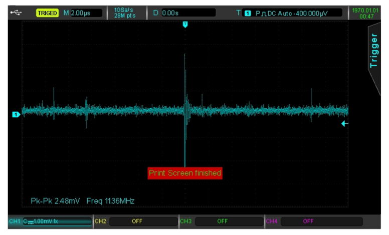
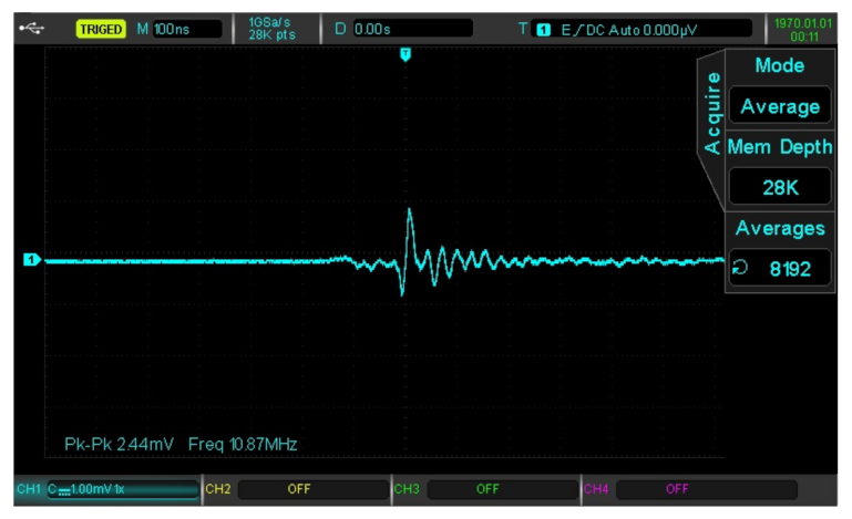
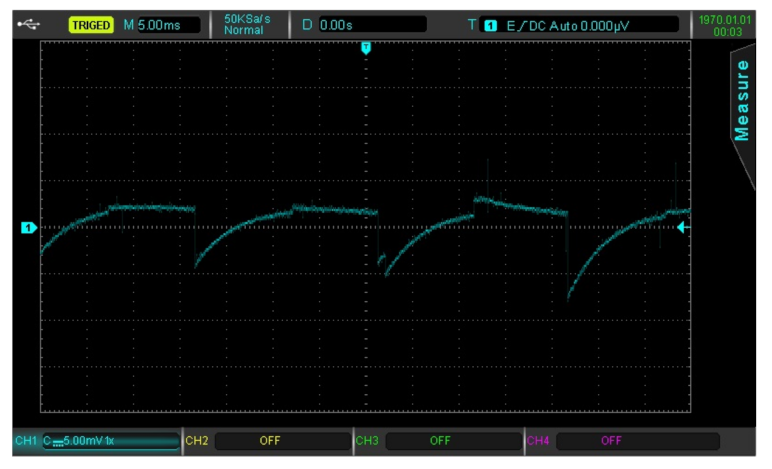
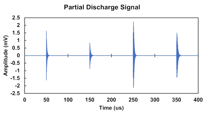
3. Generation of the Partial Discharge Signal

The idea is to generate a PD signal in the lab that resembles those occurring in high voltage cables, due to internal defects. For this purpose, samples of 132 kV, 1200 mm ${}^2$ copper conductor, XLPE insulation, lead sheath, and HDPE jacket cables were provided by Elsewedy Cables. These samples were confirmed to be PD-free using the company’s shielded PD lab at the main cables production factory, which was done according to IEC 62067 [5].

The samples were prepared as shown in Figure 3. The outer jacket, the sheath and the outer semiconductor were removed by 200 mm from both sides, leaving only the conductor and the XLPE insulation. This modification permits raising the voltage to a level suitable for developing a discharge. An artificial cylindrical void measuring 2 mm in diameter and 10 mm in depth is imposed on the cable sample in the radial direction.

The cable is connected to the output of a 1 kVA, 220 V/60 kV testing transformer that is equipped with a variac for changing the output voltage. A Rogowski coil (RC) is placed around the connection between the cable sheath and the ground. Both a self-design and a commercially available RC was used in the experiment. The self-design RC is a 3.1-inch diameter with 20 turns. The gain at 10 MHz was tested to be 0.334 V/A or −9.52 dB. The commercially available RC was an Accuenergy 14.53-inch flexible RC, and its gain at 10 MHz is 0.072 V/A or −22.81 dB. Results by both RCs showed substantial agreement. The output of the RC is connected to a 4-channel 100 MHz 1GSa/s oscilloscope. In order to reduce the effect of corona discharge and raise the corona inception voltage to a level above the testing voltage level, the ends of connecting cables and all connections were made smooth. The ends of the main cable under test were also fitted with two conductive spheres to make the electric field around them uniform as shown in Figure 4.

An isolated HV supply is connected between the cable conductor and the sheath. A Rogowski coil is connected across the connection with the sheath, and the voltage is raised until PD is detected on the oscilloscope. Figure 5 shows a schematic diagram of the experimental setup. It was noticed that the PD signal starts appearing at 9 kV, so the test voltage was raised to 10 kV and held at that value without raising it any further to ensure that the discharge is corona-free. In this experiment, audible corona started at around 18 kV.

Figure 6 shows the acquired PD signal that is generated, due to the presence of a void inside the insulation of the cable. It appears as multiple pulses along the span of the power cycle. Although the acquired signal has some white noise superimposed on it, the PD pulses can be distinctively seen since the noise amplitude does not exceed 10% of the PD pulse amplitude. By zooming on one of those pulses, those pulses clearly appear in the form of damped oscillations as shown in Figure 7. This PD type was the common type generated, due to the internal cavity defect inside power cables, which was detected using an inductive sensor, i.e., RC or HFCT [41,42,43]. By running multiple tests, it was found that the amplitude of those pulses ranged from 1 mV to 2.5 mV with the frequency detected by the oscilloscope ranging between 10 MHz to 12 MHz, so 11 MHz was selected for the computer-generated PD pulses.

It is worth noting that upon raising the voltage above the corona inception voltage (about 18 kV), the PD pulse starts taking a shape that resembles the saw-tooth waveform, indicating that above this voltage, the discharge type is predominantly due to external corona discharge, hence further proving that the damped oscillatory waveform acquired below this voltage level is indeed due to an internal PD. Figure 8 shows the pulses acquired due to corona discharge, which is clearly different from the PD pulses due to internal discharge [42].

To control the exact noise level added to the signal, the detected signal was not imported directly, as it contains some degree of noisiness. Instead, a completely clean PD signal is replicated, using a piece-wise equation that follows the mathematical model of a damped oscillation as in (3).

$$S\left(n\right)=A_1{e}^{\left(\frac{n-\varphi }{\lambda }\right)}sin\left(\omega (n-\varphi )\right).$$

(3)

where $S\left(n\right)$ is the generated PD signal, n is the discrete-time sample, $A_1$ is the amplitude, $\varphi$ is the phase shift, $\lambda$ is the damping coefficient, and $\omega$ is the angular frequency.

This computer-aided replication further serves the purpose of generalizing the PD signal to include different insulation defects in terms of size, shape, and location, and thus, strengthens the findings of this paper. The simulated PD signal is shown in Figure 9. It is made up of four pulses with amplitudes of 1.5 mV, 1 mV, 2.5 mV, and 1.5 mV at a frequency of 11 MHz. The sampling frequency is 20 MHz.

4. Denoising of the Partial Discharge Signal

In order to simulate the heavy-noise environment that is present on-site, the three major types of noises need to be generated and added to the PD signal.

4.1. Modeling of Noises Present On-Site

The most common types of noises that can be superimposed on the detected PD signal are Gaussian white noise, discrete spectral interference, and stochastic pulse interference. To include these types of noises in the study, they are modeled mathematically as follows:

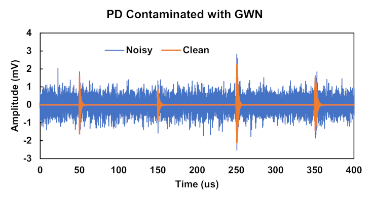
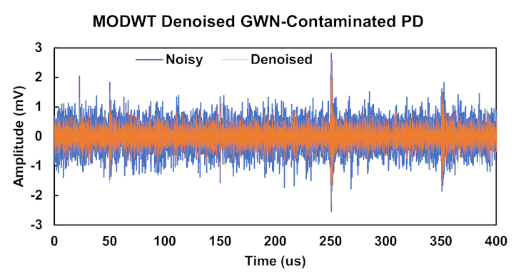
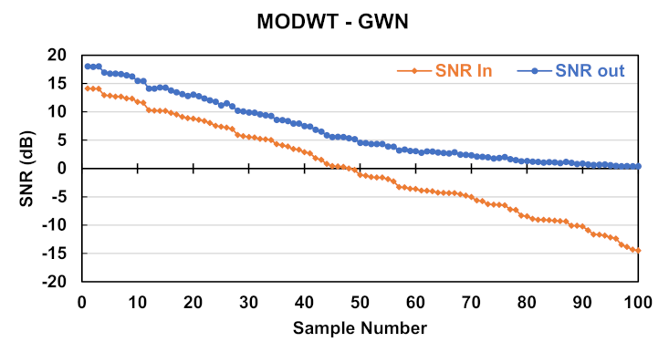
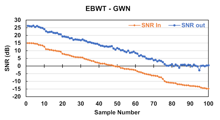
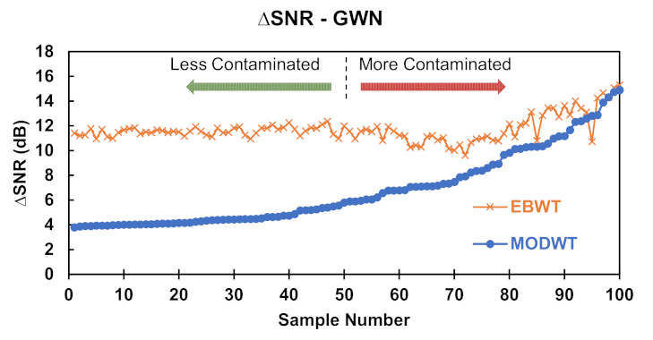
4.1.1. Gaussian White Noise (GWN)

Zero-mean Gaussian white noise that originates from amplifiers in addition to the ambiance. It is defined as a generalized stationary stochastic process with constant spectral density [44].

In this paper, the signal-to-noise ratio (SNR) of the GWN was randomly varied from 15 dB (lightly contaminated) to −15 dB (heavily contaminated).

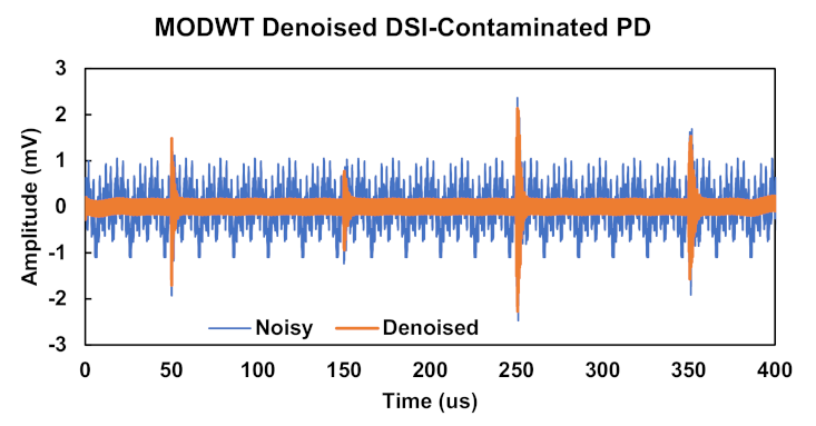
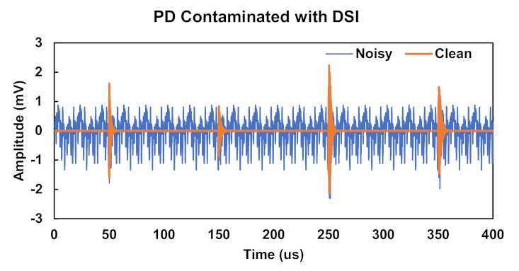
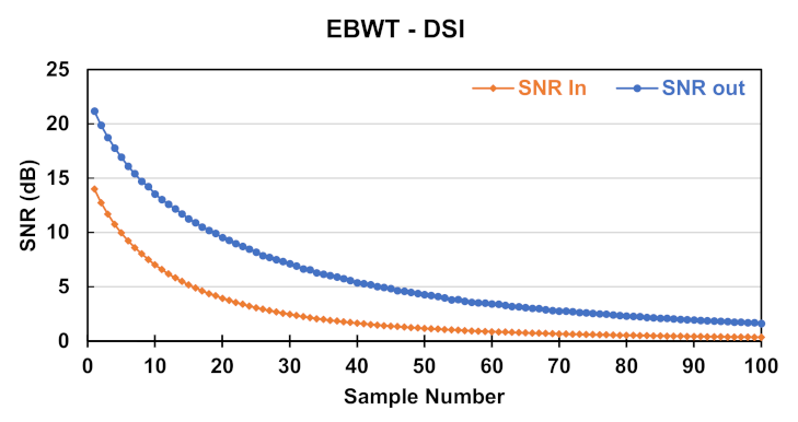
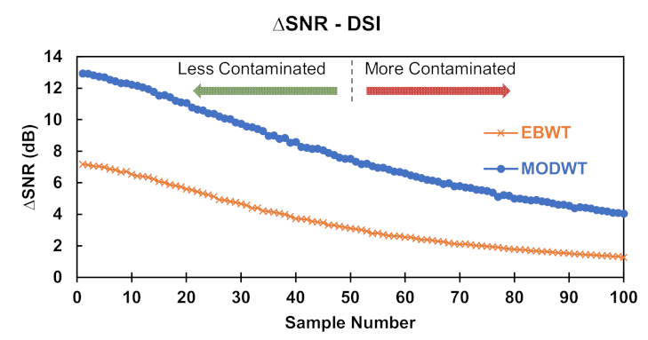
4.1.2. Discrete Spectral Interference (DSI)

DSI noises emanate from communication signals, such as power line carrier communication and radio transmission. The DSI can be classified as narrow-band noise. This type of noise can be modeled as a summation of sinusoids with frequencies ranging from 50 kHz to 1.4 MHz [27,45,46,47]. The mathematical model is as follows:

$$DSI\left(\mathrm{n}\right)=A_2\sum _1^{J}sin(2\pi f_{i}n-{\varphi }_i).$$

(4)

where DSI(n) is the noise, $A_2$ is the amplitude, $f_i$ is the frequency, and ${\varphi }_i$ is a random phase shift. J is the number of sinusoids that form the noise, which is selected as 11 in this study.

The DSI in this paper is formed of 11 sinusoids of random phase shifts; frequencies of 50 kHz, 100 kHz, 200 kHz, 300 kHz, 400 kHz, 500 kHz, 600 kHz, 700 kHz, 800 kHz, 900 kHz, and 1.4 MHz; and an amplitude range of 0.01 mV to 0.2 mV.

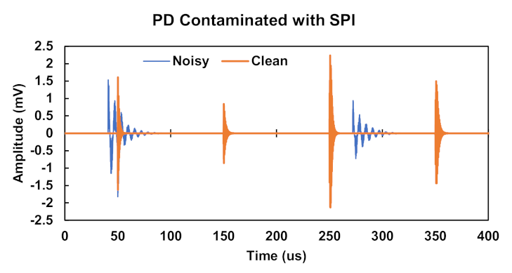
4.1.3. Stochastic Pulse Shaped Interference (SPI)

SPI can be detected, due to random switching and arcing, power electronics firing, rotating machinery brushes, and corona discharge. Since it can span a wide range of frequencies, it can be classified as wide-band noise. The mathematical model for SPI is as follows [27,47,48]:

$$SPI\left(\mathrm{n}\right)=A_3{e}^{(-{\lambda }_3(n-{\varphi }_3))}cos\left({\omega }_3(n-{\varphi }_3)\right).$$

(5)

where SPI(n) is the noise, $A_3$ is a randomly generated amplitude, ${\lambda }_3$ is the damping constant, ${\omega }_3$ is the frequency of the noise, and ${\varphi }_3$ is a randomly generated phase shift.

The SPI in this study is simulated by two pulses with random phase occurrence in the power cycle, frequency of 1 MHz, and amplitude randomly varied between 0.15 mV and 1.8 mV.

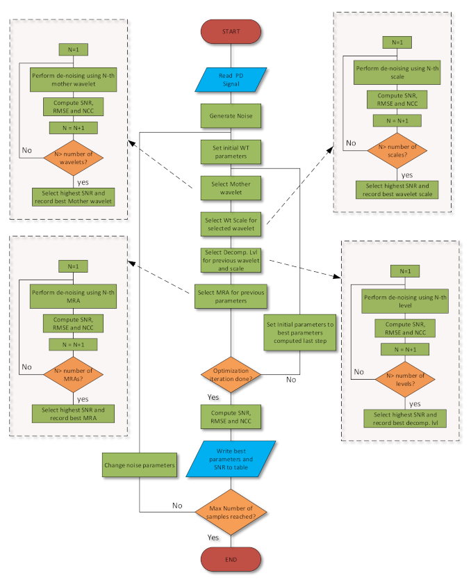
4.2. Denoising Algorithm

The process of denoising the contaminated signal is as follows:

• A PD signal is generated as described in Section 3.
• A random noise is generated and combined with the PD signal from the previous step.
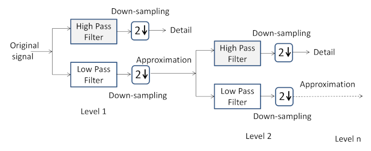
• The contaminated PD signal is then fed to an algorithm that applies the MODWT denoising, using random wavelet parameters (i.e., mother wavelet, level, wavelet scale, and combination of MRA).
• For each category of these parameters, one specific parameter is changed (e.g., the mother wavelet is sequentially varied (between Symlets, Daubechies, bi-orthogonal, Fejer–Korovkin, and Coiflets), the level is varied from 1 to 8, etc.) and the SNR is calculated. The best parameter corresponding to the highest SNR value is recorded.
• Using the best parameter in a specific category, the next category of parameters is changed in succession, recording the best parameter as in the previous step.
• Using the best parameter in each category, the whole process is repeated to improve the accuracy of the denoising.
• The final denoised signal is outputted along with the output SNR.

This process is repeated for a sample of one hundred randomly generated noises, and the results are displayed in the following section. Figure 10 shows the flow chart of the process described above.

5. Results and Discussion

In order to judge the performance of the MODWT, both input and output signal-to-noise ratios (SNR) were calculated for each contaminated signal using (6) and (7). The improvement in SNR values $\Delta SNR$ were also calculated using (8).

$$SN{R}_{In}=10{log}_{10}\left(\frac{{\displaystyle \sum _{n=1}^K}{\left(S\right(n\left)\right)}^2}{\sum _{n=1}^K{\left(N\right(n\left)\right)}^2}\right).$$

(6)

$$SN{R}_{Out}=10{log}_{10}\left(\frac{{\displaystyle \sum _{n=1}^K}{\left(S\right(n\left)\right)}^2}{{\sum }_{n=1}^K{\left(Q\right(n)-S(n\left)\right)}^2}\right).$$

(7)

$$\Delta SNR=SN{R}_{Out}-SN{R}_{In}.$$

(8)

where $S\left(n\right)$ is the clean PD signal, $N\left(n\right)$ is the noise, $Q\left(n\right)$ is the denoised signal, and K is the total number of samples.

Another way of judging the performance is by calculating the input and output normalized correlation coefficients (NCC). The NCC can measure the degree of similarity between the signal and the clean PD. It acquires values from −1 to 1, in which 1 means exactly the same, −1 means exactly inverted, and 0 means orthogonal. Input and output NCCs can be calculated, using (9) and (10), respectively.

$$NC{C}_{In}=\frac{{\displaystyle \sum _{i=1}^n}S\left(n\right)\left(S\right(n)+N(n\left)\right)}{\sqrt{{\displaystyle \sum _{i=1}^n}{S\left(n\right)}^2{\displaystyle \sum _{i=1}^n}{\left(S\right(n)+N(n\left)\right)}^2}}.$$

(9)

$$NC{C}_{Out}=\frac{{\displaystyle \sum _{i=1}^n}\left(S\right(n\left)\right)\left(Q\right(n\left)\right)}{\sqrt{{\displaystyle \sum _{i=1}^n}{S\left(n\right)}^2{\displaystyle \sum _{i=1}^n}{Q\left(n\right)}^2}}.$$

(10)

Running the algorithms and changing the mother wavelet revealed that selecting Daubechies wavelets almost always gave better results than other wavelets, with symlet wavelets coming second in terms of SNR improvements. It is also worth noting that running the MODWT nested algorithm described in the flowchart (Figure 10) consumed less time than running the EBWT nested algorithm. This is due to the lower number of categories to change parameters within in order to achieve the best performance, which is four in the case of MODWT and six in the case of EBWT. On an Intel Core i7-7700HQ CPU, 2.80 GHz, 3.8 GHz single-core boost, the EBWT algorithm needed 183 s to complete the denoising of the 100 samples, while the MODWT needed 171 s to complete the same task. However, these times will be different on different machines. While it is not a big difference, considering this is used in continuous online monitoring, the difference in time will add up over a long period.

Figure 11 shows a sample of the simulated PD signal that was contaminated with DSI. The SNR, in this case, was 0.35 dB, whereas the NCC was 0.28. The denoised signal using MODWT is shown in Figure 12. The SNR, in that case, increased to 4.39 dB with an improvement of 4.04 dB. The NCC also increased to 0.79. It can be noted that the amplitude of the denoised pulses was slightly lower than the input signal. Likewise, applying EBWT on a different sample also yielded an improvement in SNR as shown in Figure 13. In this case, the SNR of the noisy signal was 0.35 dB and the SNR of the denoised signal shown in Figure 13 was 1.61 dB. Additionally, the input NCC was 0.28, and the output was 0.55. Nevertheless, the noise in the denoised signal appears to be lower. A careful inspection would reveal that the lower improvement in SNR and NCC values were due to some distortion in the PD signal’s amplitude and spectrum (can be seen in the second pulse at 150 $\mathrm{\mu }$s in the figure). Comparing the amplitudes of the PD pulses after denoising reveals that since the MODWT-based algorithm has a lower impact on the amplitude, it has an advantage in condition monitoring of insulation reflecting a more accurate indication of the severity of the PD.

The results of applying the MODWT algorithm on samples of PD contaminated with DSI noise type are comparatively shown in Figure 14, whereas the results of applying the EBWT algorithm on the same number of samples are shown in Figure 15. The vertical axis shows the input and the output SNR and the horizontal axis shows the index of the sample.

Inspecting Figure 14 shows that the maximum improvement $\Delta SNR$ was about 12.93 dB and the minimum was 4.04 dB, with an average of 7.89 dB. In comparison, applying EBWT reveals lower improvement in SNR values than MODWT, as the maximum and minimum $\Delta SNR$ were 7.17 dB and 1.25 dB, respectively. The average was 3.56 dB. In addition, comparing Figure 14 and Figure 15 shows that the performance of the EBWT algorithm declines more with heavy noise content, compared to the MODWT algorithm.

To further compare the performance of both algorithms, the $\Delta SNR$ values are combined in Figure 16. From this figure, it is obvious that the improvement in SNR values achieved by the MODWT-based algorithm is higher than that of the EBWT in all the studied cases. The performance for both methods decreased as the signal noisiness increased, but the MODWT performance remained in the lead.

Figure 17 shows an individual sample of a GWN-contaminated PD signal, whereas the denoised signal using MODWT is also shown in Figure 18. The SNR of the noisy input signal was −10.12 dB and the NCC was 0.28. After denoising with the MODWT algorithm, the SNR of the output signal increased to 0.85 dB, with an improvement in $\Delta SNR$ of 10.97 dB, and the NCC also increased to 0.42. A small drop in amplitude is also noticed. This shows that for GWN-heavy contamination, the MODWT algorithm could decrease the noise SNR, while reserving the features of the PD signal.

To assess the performance on a wide range of contamination levels, the results of using MODWT and EBWT on the 100 samples contaminated with GWN are displayed in Figure 19 and Figure 20, respectively. The SNR output value compared to the input shows that both are on par with a slight lead in favor of EBWT in terms of average performance. The MODWT maximum $\Delta SNR$ was about 14.89 dB and the minimum was 3.8 dB, with an average improvement of around 6.8 dB, whereas the EBWT had a maximum $\Delta SNR$ of 15.29 dB and a minimum of 9.6 dB, with an average of 11.7 dB. This is further emphasized by comparing the $\Delta SNR$ of the two algorithms simultaneously in Figure 21. In most cases, the MODWT-based algorithm performance lags behind that of the EBWT, with the difference becoming narrower until they overlap; the performance can be considered similar for lower input SNR values (i.e., highly contaminated signals).

Furthermore, Figure 22 shows a case of the PD signal that is contaminated with a randomly generated SPI noise. It is evident from the figure that both the clean PD and the SPI noise are similar in shape. The input SNR, in this case, was 3.4 dB. The output of applying the MODWT denoising algorithm on this sample is shown in Figure 23. It appears that the noise, namely, at 40 and 270 $\mathsf{\mu }$s, diminished significantly, while the PD signal remained intact. Another important observation to note is that the MODWT algorithm was able to differentiate between the SPI pulse at 40 $\mathsf{\mu }$s and the clean PD pulse at 50 $\mathsf{\mu }$s, even though they are overlapping. The SNR of this denoised signal was 12.18 dB, with a $\Delta SNR$ 8.87 dB. The NCC also increased from 0.73 for the noisy signal to 0.96 for the denoised signal.

Figure 24 shows the results of using the MODWT to denoise a sample of one hundred signals that are contaminated by a randomly generated SPI noise type. From the figure, it can be seen that the output SNR is higher than the input in all samples. It can be noted from the average slopes of both curves that the performance remains constant, even with heavily noisy signals (i.e., low input SNR). The maximum $\Delta SNR$ was 10.8 dB, whereas the minimum $\Delta SNR$ was 7.7 dB with an average of 9.4 dB.

To compare, Figure 25 shows the results of applying the EBWT on the same 100 samples that were used with the MODWT. It is clear from the figure that the EBWT has little to no effect on the PD signals. The maximum was 0.015 dB and the minimum was 0.0045 dB with an average of 0.0089 dB. This can be attributed to the significant similarity between the SPI noise type and the clean PD signal, which proves challenging for most denoising methods.

Putting the $\Delta SNR$ values for both methods next to each other in Figure 26 further confirms the conclusion that the MODWT has the lead on denoising SPI, while the EBWT had almost no effect on the noisy signal, which holds true for lightly as well as heavily contaminated signals. The average $\Delta SNR$ for the MODWT was 9.41 dB, while the average for the EBWT was 0.01 dB.

Finally, to test the performance in a real-life situation, where noises may occur concurrently, the performance was tested against a PD signal that was contaminated with all three types of noises simultaneously. Figure 27 shows a sample of a contaminated signal of this type after applying the MODWT-based algorithm to denoise it. The input SNR, in that case, was 0.43 dB and the input NCC was 0.31. After denoising, the SNR increased to 5.39 dB and the NCC increased to 0.84.

Another sample contaminated with all three noise types after applying the EBWT to denoise it is shown in Figure 28. In this sample, the input SNR was 1.23 dB and the NCC was 0.49. The SNR and NCC after denoising were 2.98 dB and 0.72, simultaneously.

Similar to the individually contaminated cases, one hundred samples of the PD signal contaminated with randomly generated DSI, GWN, and SPI simultaneously were used to test and compare the performance of both the MODWT and the EBWT algorithms. Figure 29 shows the output SNR versus the input SNR for the MODWT-based algorithm, whereas Figure 30 shows the output SNR versus the input SNR for the EBWT. For the MODWT cases, the maximum $\Delta SNR$ was 6.37 dB and the minimum was 0.18 dB with an average of 2.66 dB. For the EBWT cases, the maximum $\Delta SNR$ was 3.25 dB, the minimum $\Delta SNR$ was −1.83 dB, and the average was 1.11 dB.

Again, for a more clear comparison, Figure 31 shows the $\Delta SNR$ for both methods on the same vertical axis. The MODWT algorithm has better results for most cases with an average $\Delta SNR$ of 2.66 dB, compared to the EBWT that has an average $\Delta SNR$ of only 1.11 dB. Moreover, as the signal’s input SNR decreases and the signal becomes noisier, the MODWT algorithm holds a positive $\Delta SNR$. This is not the case for EBWT, as the SNR of the signal deteriorates, indicating that it has a negative effect on the signal.

The summary of the improvements in SNR values ($\Delta SNR$) for all previous cases as well as the average values of NCC calculated for the same cases are displayed in

Table 1. $\Delta SNR$ values and average values of normalized correlation coefficient for both MODWT and EBWT.

		MODWT	EBWT		MODWT	EBWT
SPI	Min. SNR	7.702788	0.004511	NCC In	0.802583	0.805013
	Max. SNR	10.81265	0.015302	NCC Out	0.979162	0.805224
	Avg. SNR	9.409513	0.008991
DSI	Min. SNR	4.042913	1.258958	NCC In	0.541432	0.541559
	Max. SNR	12.93946	7.176028	NCC Out	0.917836	0.788407
	Avg. SNR	7.890591	3.561922
GWN	Min. SNR	3.804889	9.617872	NCC In	0.650192	0.619359
	Max. SNR	14.89552	15.29064	NCC Out	0.759157	0.829106
	Avg. SNR	6.815711	11.71665
All 3	Min. SNR	0.175361	−1.833993	NCC In	0.377073	0.375178
	Max. SNR	6.369339	3.253451	NCC Out	0.665364	0.572604
	Avg. SNR	2.661951	1.113674

. The matching trend between NCC and SNR values confirms the previous results.

6. Conclusions

In this paper, a denoising algorithm based on the MODWT was developed that aims at the best possible PD signal improvement. The algorithm was applied to 100 random samples that simulate degrees of noisiness, and the output was compared to the EBWT denoising method to assess its performance. It is concluded that the proposed MODWT algorithm is a viable method of denoising PD signals in noise-heavy sites. It performs better than the EBWT in denoising SPI as well as DSI-contaminated PD signals. Moreover, the MODWT algorithm is also better in denoising all three noise types when they exist simultaneously. This superiority is manifested by the following:

• The proposed MODWT algorithm consumes less computational time, which is considered an advantage to insulators’ condition monitoring.
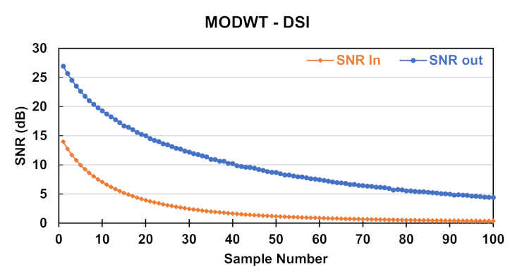
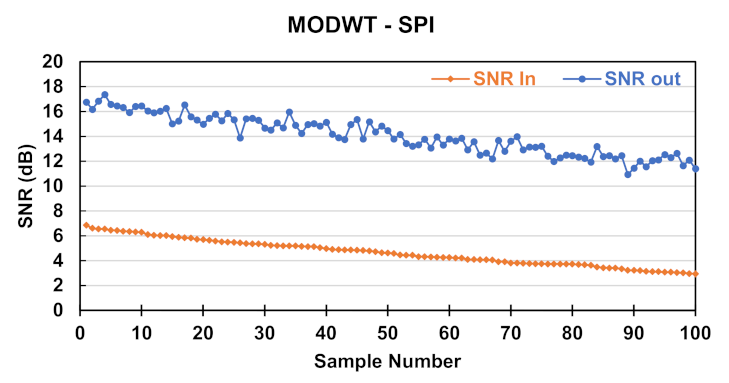
• The MODWT-based algorithm improved the SNR values of the signal by an average of 9.4 dB, 7.89 dB, and 6.81 dB after denoising SPI-, DSI-, and GWN-contaminated PD signals, respectively. This signifies the ability of the proposed algorithm to decrease the noisiness of the signal.
• The MODWT-based algorithm also increased the values of the NCC after denoising SPI, DSI, and GWN-contaminated PD signals to 0.97, 0.91, and 0.76, respectively, which indicates the ability to preserve the features of the PD signal.
• Moreover, the MODWT-based algorithm had a small impact on the features of the signal (i.e., amplitude and spectrum). This proves advantageous in assessing the severity of the PD and hence, the condition of the insulation.
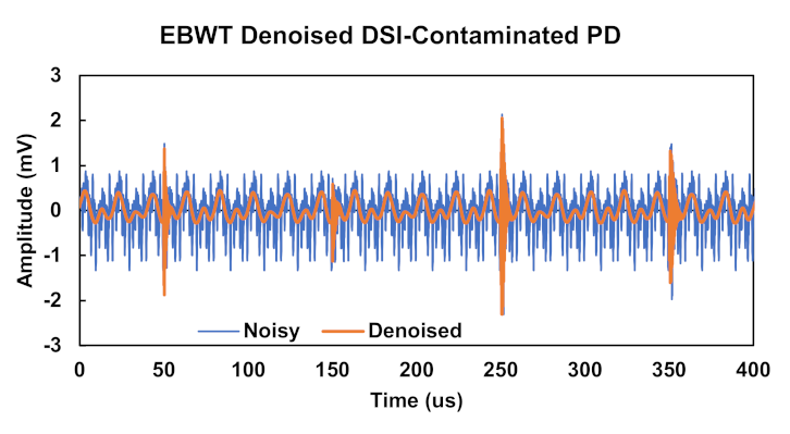
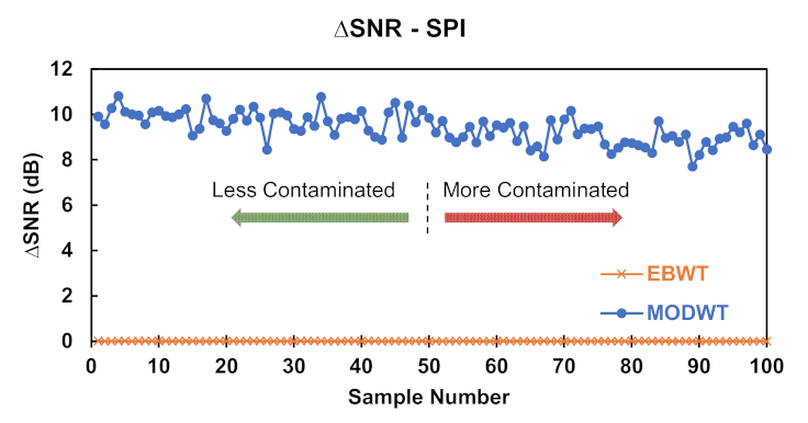
• Comparing the MODWT-based algorithm to the EBWT shows better results for the former over the latter after denoising SPI-contaminated signals and DSI-contaminated signals in terms of SNR and NCC values.
• While the EBWT algorithm showed slightly better results in denoising GWN-contaminated PD, as the contamination level increases, the performance difference over the MODWT algorithm decreases substantially until the performance overlaps and becomes very similar for very heavy contamination.
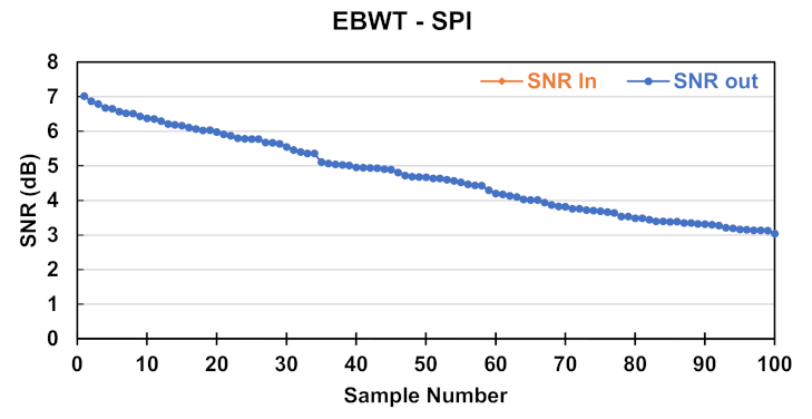
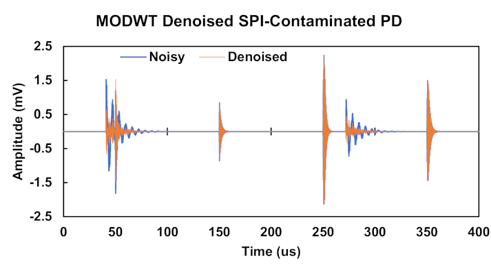
• The most obvious point of strength that differentiates MODWT from EBWT is the very good results in denoising SPI-contaminated PD, while the EBWT completely failed to remove this noise type.
• The MODWT-based algorithm could differentiate between the PD signal and the similarly shaped SPI, providing high $\Delta SNR$ and NCC, even when there is a visible overlap between the PD pulse and the SPI pulse.
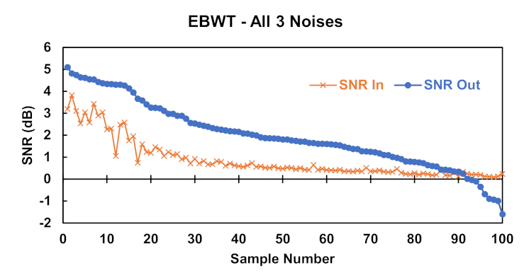
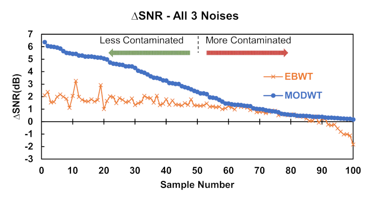
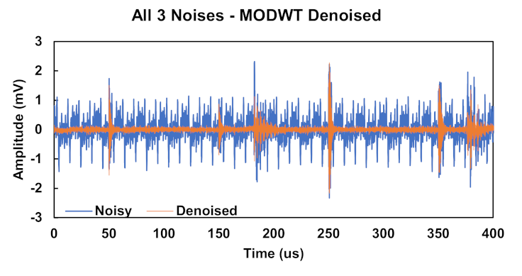
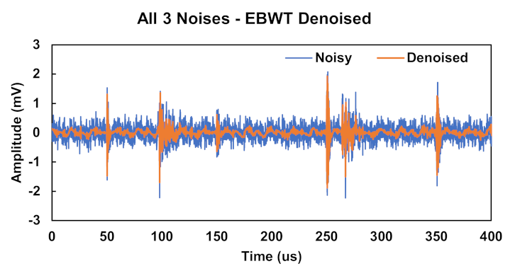
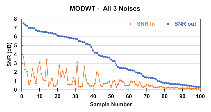
• In the case of concurrently existing noises, the MODWT algorithm achieved better results for both lightly contaminated and heavily contaminated signals.

References

1. Gan, L. Insulation Coordination in the Alberta Interconnected Electric System; Technical Report; Alberta Electric System Operator: Calgary, AB, Canada, 2015. [Google Scholar]
2. Zhou, S.; Tang, J.; Pan, C.; Luo, Y.; Yan, K. Partial Discharge Signal Denoising Based on Wavelet Pair and Block Thresholding. IEEE Access 2020, 8, 119688–119696. [Google Scholar] [CrossRef]
3. Abdel-salam, M.; Anis, H.; El-Morshedy, A.; Radwan, R. High Voltage Engineering (Theory and Practice), 2nd ed.; Marcel Dekker, Inc.: New York, NY, USA, 2000; pp. 1–743. [Google Scholar] [CrossRef]
4. IEC. Electrical Test Methods for Electric Cables-Part 3: Test Methods for Partial Discharge Measurements on Lengths of Extruded Power Cables; Standard IEC 60885-3:2015; International Electrotechnical Commission: Geneva, Switzerland, 2015. [Google Scholar]
5. IEC. Power Cables with Extruded Insulation and Their Accessories for Rated Voltages Above 150 kV (Um = 170 kV) up to 500 kV (Um = 550 kV)-Test Methods and Requirementss; Standard IEC 62067:2011; International Electrotechnical Commission: Geneva, Switzerland, 2011. [Google Scholar]
6. Shafiq, M.; Kauhaniemi, K.; Robles, G.; Isa, M.; Kumpulainen, L. Online condition monitoring of MV cable feeders using Rogowski coil sensors for PD measurements. Electr. Power Syst. Res. 2019, 167, 150–162. [Google Scholar] [CrossRef]
7. Tulsani, H.; Gupta, R. Impact of Different Wavelets for Discrete and Shift Invariant Wavelet Transforms on Partial Discharge Signal Denoising. Int. J. Eng. Technol. Innov. 2014, 1, 13–21. [Google Scholar]
8. Vidya H.A, V.H.; Tyagi, B.; V Krishnan, V.K.; Mallikarjunappa, K.M. Removal of Interferences from Partial Discharge Pulses using Wavelet Transform. Telecommun. Comput. Electron. Control 2015, 9, 107. [Google Scholar] [CrossRef]
9. Suganya, G.; Jayalalitha, S.; Kannan, K.; Venkatesh, S. Survey of de-noising techniques for partial discharge interferences. ARPN J. Eng. Appl. Sci. 2017, 12, 414–427. [Google Scholar]
10. Soltani, A.A.; El-Hag, A. Denoising of radio frequency partial discharge signals using artificial neural network. Energies 2019, 12, 3485. [Google Scholar] [CrossRef] [Green Version]
11. Ashtiani, M.; Shahrtash, S. Partial discharge de-noising employing adaptive singular value decomposition. IEEE Trans. Dielectr. Electr. Insul. 2014, 21, 775–782. [Google Scholar] [CrossRef]
12. Rojas-Moreno, M.V.; Robles, G.; Martinez-Tarifa, J.M.; Fresno, J.M. Ensemble Empirical Mode Decomposition for the denoising of partial discharges measured in UHF. In Proceedings of the 2016 IEEE International Conference on Dielectrics, ICD 2016, Montpellier, France, 3–7 July 2016; Volume 2, pp. 963–966. [Google Scholar] [CrossRef]
13. Jin, T.; Li, Q.; Mohamed, M.A. A Novel Adaptive EEMD Method for Switchgear Partial Discharge Signal Denoising. IEEE Access 2019, 7, 58139–58147. [Google Scholar] [CrossRef]
14. Zhong, J.; Bi, X.; Shu, Q.; Chen, M.; Zhou, D.; Zhang, D. Partial Discharge Signal Denoising Based on Singular Value Decomposition and Empirical Wavelet Transform. IEEE Trans. Instrum. Meas. 2020, 69, 8866–8873. [Google Scholar] [CrossRef]
15. Yusoff, N.A.; Isa, M.; Hamid, H.; Adzman, M.R.; Rohani, M. Denoising Technique for Partial Discharge Signal: A Comparison Performance between Artificial Neural Network, Fast Fourier Transform and Discrete Wavelet Transform. In Proceedings of the 2016 IEEE International Conference on Power and Energy (PECon), Melaka, Malaysia, 28–29 November 2016; pp. 311–316. [Google Scholar]
16. Guzmán, I.a.C.; Oslinger, J.L.; Nieto, R.D. Wavelet denoising of partial discharge signals and their pattern classification using artificial neural networks and support vector machines [Filtrado wavelet de descargas parciales y su clasificación de patrones usando redes neuronales artificiales y máq. DYNA 2017, 84, 240–248. [Google Scholar] [CrossRef]
17. Soltani, A.A.; El-Hag, A. A new radial basis function neural network-based method for denoising of partial discharge signals. Meas. J. Int. Meas. Confed. 2021, 172, 108970. [Google Scholar] [CrossRef]
18. Mas’ud, A.A.; Albarracín, R.; Ardila-Rey, J.A.; Muhammad-Sukki, F.; Illias, H.A.; Bani, N.A.; Munir, A.B. Artificial neural network application for partial discharge recognition: Survey and future directions. Energies 2016, 9, 574. [Google Scholar] [CrossRef] [Green Version]
19. Li, S.; Sun, S.; Shu, Q.; Chen, M.; Zhang, D.; Zhou, D. Partial discharge signal denoising method based on frequency spectrum clustering and local mean decomposition. IET Sci. Meas. Technol. 2020, 14, 853–861. [Google Scholar] [CrossRef]
20. Yang, X.; Cai, Y.; Zhang, J.; Cheng, L.; Wang, F. Periodic narrow-band noise denoising of partial discharge signal through time-frequency analysis. In Proceedings of the 2020 IEEE 4th Conference on Energy Internet and Energy System Integration: Connecting the Grids Towards a Low-Carbon High-Efficiency Energy System, EI2 2020, Wuhan, China, 30 October–1 November 2020; pp. 2248–2251. [Google Scholar] [CrossRef]
21. Ergen, B. Signal and Image Denoising Using Wavelet Transform. In Advances in Wavelet Theory and Their Applications in Engineering, Physics and Technology; IntechOpen: Rijeka, Croatia, 2012. [Google Scholar] [CrossRef] [Green Version]
22. Ning, T.; Huang, C.h.; Jensen, J.A.; Wong, V.; Sheet, L. Application of Discrete-Wavelet Transform Compression in Wafer Fabrication. In Proceedings of the 2014 12th International Conference on Signal Processing (ICSP), Hangzhou, China, 19–23 October 2014; pp. 2272–2276. [Google Scholar]
23. Saini, S.; Dewan, L. Application of discrete wavelet transform for analysis of genomic sequences of Mycobacterium tuberculosis. SpringerPlus 2016, 5, 64. [Google Scholar] [CrossRef] [Green Version]
24. Ma, X.; Zhou, C.; Kemp, I.J. Interpretation of wavelet analysis and its application in partial discharge detection. IEEE Trans. Dielectr. Electr. Insul. 2002, 9, 446–457. [Google Scholar] [CrossRef] [Green Version]
25. Zhou, X.; Zhou, C.; Kemp, I.J. An Improved Methodology for Application of Wavelet Transform to Partial Discharge Measurement Denoising. IEEE Trans. Dielectr. Electr. Insul. 2005, 12, 586–594. [Google Scholar] [CrossRef]
26. Yang, X.; Cai, Y.; Zhang, J.; Cheng, L.; Wang, F. Denoising of partial discharge signal by common factor method and wavelet thresholding. In Proceedings of the 2020 IEEE 4th Conference on Energy Internet and Energy System Integration: Connecting the Grids Towards a Low-Carbon High-Efficiency Energy System, EI2 2020, Wuhan, China, 30 October–1 November 2020; pp. 2252–2255. [Google Scholar] [CrossRef]
27. Ma, X.; Zhou, C.; Kemp, I.J. Investigation into The Use Of Wavelet Theory For Partial Discharge Pulse Extraction in Electrically Noisy Environments. In Proceedings of the Eighth International Conference on Dielectric Materials, Measurements and Applications, Edinburgh, UK, 17–21 September 2000; Volume 4, pp. 123–126. [Google Scholar]
28. Luo, L.; Han, B.; Chen, J.; Sheng, G.; Jiang, X. Partial Discharge Detection and Recognition in Random Matrix Theory Paradigm. IEEE Access 2017, 5, 8205–8213. [Google Scholar] [CrossRef]
29. Shams, M.A.; El-Shahat, M.; Anis, H.I. Detection and de-noising of PD signal contaminated with stochastic pulse interference using maximal overlap discrete wavelet transform. In Proceedings of the 2020 IEEE 3rd International Conference on Dielectrics (ICD), Valencia, Spain, 5–31 July 2020; pp. 834–837. [Google Scholar] [CrossRef]
30. Cornish, C.R.; Bretherton, C.S.; Percival, D.B. Maximal overlap wavelet statistical analysis with application to atmospheric turbulence. Bound.-Layer Meteorol. 2006, 119, 339–374. [Google Scholar] [CrossRef]
31. Polanco-Martínez, J.M.; Abadie, L.M. Analyzing crude oil spot price dynamics versus long term future prices: A wavelet analysis approach. Energies 2016, 9, 1089. [Google Scholar] [CrossRef] [Green Version]
32. Seo, Y.; Choi, Y.; Choi, J. River stage modeling by combining maximal overlap discrete wavelet transform, support vector machines and genetic algorithm. Water 2017, 9, 525. [Google Scholar] [CrossRef] [Green Version]
33. AL-Musaylh, M.S.; Deo, R.C.; Li, Y. Electrical energy demand forecasting model development and evaluation with maximum overlap discrete wavelet transform-online sequential extreme learning machines algorithms. Energies 2020, 13, 2307. [Google Scholar] [CrossRef]
34. Wang, Y.; Zhang, B.; Ding, F.; Ren, H. Estimating Dynamic Motion Parameters with an Improved Wavelet Thresholding and Inter-Scale Correlation. IEEE Access 2018, 6, 39827–39838. [Google Scholar] [CrossRef]
35. Satish, L.; Nazneen, B. Wavelet-based denoising of partial discharge signals buried in excessive noise and interference. IEEE Trans. Dielectr. Electr. Insul. 2003, 10, 354–367. [Google Scholar] [CrossRef] [Green Version]
36. Johnstone, I.M.; Silverman, B.W. Empirical bayes selection of wavelet thresholds. Ann. Stat. 2005, 33, 1700–1752. [Google Scholar] [CrossRef] [Green Version]
37. Jansen, M.; Bultheel, A. Empirical bayes approach to improve wavelet thresholding for image noise reduction. J. Am. Stat. Assoc. 2001, 96, 629–639. [Google Scholar] [CrossRef]
38. Kim, C.H.; Agganrval, R. Wavelet transforms in power systems: Part 1 General introduction to the wavelet transforms. Power Eng. J. 2000, 14, 81–88. [Google Scholar]
39. Song, X.; Zhou, C.; Hepburn, D.M.; Zhang, G.; Michel, M. Second generation wavelet transform for data denoising in PD measurement. IEEE Trans. Dielectr. Electr. Insul. 2007, 14, 1531–1537. [Google Scholar] [CrossRef]
40. Percival, D.B.; Walden, A.T. Wavelet Methods for Time SeriesAnalysis; Cambridge University Press: Cambridge, UK, 2000. [Google Scholar] [CrossRef]
41. Shafiq, M.; Kiitam, I.; Taklaja, P.; Kutt, L.; Kauhaniemi, K.; Palu, I. Identification and Location of PD Defects in Medium voltage Underground Power Cables Using High Frequency Current Transformer. IEEE Access 2019, 7, 103608–103618. [Google Scholar] [CrossRef]
42. Gomez, F.A.; la Moneda, J.O.; Vecino, F.G.; Gonzalez, M.A.S.U. A clustering technique for partial discharge and noise sources identification in power cables by means of waveform parameters. IEEE Trans. Dielectr. Electr. Insul. 2016, 23, 469–481. [Google Scholar]
43. Álvarez, F.; Garnacho, F.; Ortego, J.; Sánchez-Urán, M.Á. Application of HFCT and UHF sensors in on-line partial discharge measurements for insulation diagnosis of high voltage equipment. Sensors 2015, 15, 7360–7387. [Google Scholar] [CrossRef] [PubMed] [Green Version]
44. Marmarelis, V.Z. Nonlinear Dynamic modeling of Physiological Systems; John Wiley & Sons, Ltd.: Hoboken, NJ, USA, 2004; pp. 499–501. [Google Scholar]
45. Xie, J.; Lv, F.; Li, M.; Wang, Y. Suppressing the discrete spectral interference of the partial discharge signal based on bivariate empirical mode decomposition. Int. Trans. Electr. Energy Syst. 2017, 27, 1–17. [Google Scholar] [CrossRef]
46. Zhang, H.; Blackburn, T.R.; Phung, B.T.; Sen, D. A novel wavelet transform technique for on-line partial discharge measurements part 1: WT de-noising algorithm. IEEE Trans. Dielectr. Electr. Insul. 2007, 14, 3–14. [Google Scholar] [CrossRef]
47. Shetty, P.K.; Srikanth, R.; Ramu, T.S. Modeling and on-line recognition of PD signal buried in excessive noise. Signal Process. 2004, 84, 2389–2401. [Google Scholar] [CrossRef]
48. Zhang, H.; Blackburn, T.R.; Phung, B.T.; Sen, D. A novel wavelet transform technique for on-line partial discharge measurements part 2: On-site noise rejection application. IEEE Trans. Dielectr. Electr. Insul. 2007, 14, 15–22. [Google Scholar] [CrossRef]
Figure 1. Schematic diagram showing the process of decomposition using the DWT algorithm.
Energies 14 06540 g001
Figure 2. Schematic diagram showing the process of decomposing the signal, using the MODWT algorithm.
Energies 14 06540 g002
Figure 3. Tested 132 kV cable sample. The outer jacket, sheath, and semi-conductive screen were removed from the sides. A void in the radial direction of the cable was created.
Energies 14 06540 g003
Figure 4. Conducting spherical terminations on each cable end is used to reduce the effect of corona discharge.
Energies 14 06540 g004
Figure 5. Laboratory setup. A testing transformer is connected between the cable conductor and the sheath. A Rogowski coil is connected across the connection with the sheath.
Energies 14 06540 g005
Figure 6. Acquired PD signal from the cable, due to an internal void using a Rogowski coil.
Energies 14 06540 g006
Figure 7. Enlarged view on one PD pulse.
Energies 14 06540 g007
Figure 8. Detected signal above the corona inception voltage. The signal resembles that due to external corona discharges.
Energies 14 06540 g008
Figure 9. Simulated partial discharge signal.
Energies 14 06540 g009
Figure 10. The proposed algorithm reads the PD signal with the noise or separately, which is then decomposed using MODWT parameters that update each iteration in a nested loop. SNR and NCC are computed for each step to estimate the performance numerically until the stop condition is reached.
Energies 14 06540 g010
Figure 11. Simulated partial discharge signal contaminated with discrete spectral interference. Signal SNR = 0.35 dB and NCC = 0.28.
Energies 14 06540 g011
Figure 12. Denoised signal while contaminated with discrete spectral interference using MODWT. Input SNR = 0.35 dB and output SNR = 4.39 dB. Input NCC = 0.28 and output NCC = 0.79.
Energies 14 06540 g012
Figure 13. Denoised DSI-contaminated signal using EBWT. Some distortion in PD signal is noticed. Input SNR = 0.34 dB, output SNR = 1.61 dB, input NCC = 0.28 and output NCC = 0.55.
Energies 14 06540 g013
Figure 14. SNR of 100 samples of PD signals contaminated with DSI. The maximum Δ S N R = 12.39 dB, the minimum = 4.04 dB, and the average = 7.89 dB.
Energies 14 06540 g014
Figure 15. Output SNR using EBWT on 100 samples of DSI contaminated PD signals. Maximum Δ S N R = 7.17 dB, Minimum Δ S N R = 1.25 dB, and average Δ S N R = 3.56 dB.
Energies 14 06540 g015
Figure 16. Δ S N R for both the MODWT and the EBWT methods. MODWT yielded better Δ S N R for all cases with an average of 7.89 dB, whereas the average Δ S N R for EBWT was 3.56 dB.
Energies 14 06540 g016
Figure 17. Simulated PD signal contaminated with GWN. SNR = −10.12 dB and NCC = 0.28.
Energies 14 06540 g017
Figure 18. Denoised PD signal contaminated with GWN using MODWT. Input SNR = −10.12 dB and output SNR = 0.85 dB. Input and output NCC = 0.28 and 0.42, respectively.
Energies 14 06540 g018
Figure 19. SNR of 100 samples of PD signals contaminated with GWN. Maximum Δ S N R = 14.89 dB, minimum Δ S N R = 3.8 dB, and average = 6.8 dB.
Energies 14 06540 g019
Figure 20. Output SNR using EBWT versus the input SNR of 100 samples of PD signals contaminated with GWN. Maximum Δ S N R = 15.29 dB and minimum Δ S N R = 9.6 dB; average = 11.7 dB.
Energies 14 06540 g020
Figure 21. Δ S N R for both MODWT and EBWT. In most cases, MODWT did not perform as well as EBWT with a lower average Δ S N R of 6.81 dB, compared to 11.71 dB for EBWT. However, the difference in performance decreases as the signal becomes more noisy until they become similar.
Energies 14 06540 g021
Figure 22. Sample of the simulated PD signal contaminated with SPI noise. Signal SNR = 3.4 dB and NCC = 0.73.
Energies 14 06540 g022
Figure 23. Denoised PD signal contaminated with SPI using MODWT. Input and output SNR = 3.4 dB and 12.18 dB, respectively. Input and output NCC = 0.73 and 0.96, respectively.
Energies 14 06540 g023
Figure 24. SNR of 100 samples of PD signals contaminated with SPI. The maximum Δ S N R = 10.8 dB and the minimum = 7.7 dB. The average Δ S N R = 9.4 dB.
Energies 14 06540 g024
Figure 25. SNR of 100 samples of PD signals contaminated with SPI using EBWT. Very little improvement was noticed. The maximum Δ S N R 0.015 dB and the minimum = 0.0045 dB with an average of 0.0089 dB.
Energies 14 06540 g025
Figure 26. Δ S N R for both the MODWT and the EBWT methods. The MODWT-based algorithm showed a clear lead in denoising SPI, whereas the EBWT had almost no effect on the noisy signal. Average Δ S N R for both the MODWT and the EBWT were 9.41 dB and 0.01 dB, respectively.
Energies 14 06540 g026
Figure 27. Denoised PD signal contaminated with the 3 types of noises simultaneously using MODWT. Input SNR = 0.43 dB and input NCC = 0.31, output SNR = 5.39 dB and output NCC = 0.84.
Energies 14 06540 g027
Figure 28. Denoised PD signal contaminated with the 3 types of noises simultaneously using EBWT. Input SNR = 1.23 dB and input NCC = 0.49, output SNR = 2.98 dB and output NCC = 0.72.
Energies 14 06540 g028
Figure 29. SNR of 100 samples of PD signals contaminated with the 3 types of noises simultaneously denoised using MODWT. The maximum Δ S N R = 6.37 dB, the minimum = 0.18 dB, and the average = 2.66 dB.
Energies 14 06540 g029
Figure 30. SNR of 100 samples of PD signals contaminated with the 3 types of noises simultaneously denoised using EBWT. The maximum Δ S N R = 3.25 dB, the minimum = −1.83 dB, and the average = 1.11 dB.
Energies 14 06540 g030
Figure 31. Δ S N R for both MODWT and EBWT. For most cases, the MODWT achieved better results. As the signal becomes more noisy, the MODWT holds positive results, while the EBWT decreases the signal SNR. Average Δ S N R for MODWT was 2.66 dB and for EBWT was 1.11 dB.
Energies 14 06540 g031