A Brief Climatology of Dunkelflaute Events over and Surrounding the North and Baltic Sea Areas

Abstract

In the coming decades, the European energy system is expected to become increasingly reliant on non-dispatchable generation such as wind and solar power. Under such a renewable energy scenario, a better characterization of the extreme weather condition ‘Dunkelflaute’, which can lead to a sustained reduction of wind and solar power, is important. In this paper, we report findings from the very first climatological study of Dunkelflaute events occurring in eleven countries surrounding the North and Baltic Sea areas. By utilizing multi-year meteorological and power production datasets, we have quantified various statistics pertaining to these events and also identified their underlying meteorological drivers. It was found that almost all periods tagged as Dunkelflaute events (with a length of more than 24 h) are in November, December, and January for these countries. On average, there are 50–100 h of such events happening in each of these three months per year. The limited wind and solar power production during Dunkelflaute events is shown to be mainly driven by large-scale high-pressure systems and extensive low-cloud coverage. Even though the possibility of simultaneous Dunkelflaute events in neighboring countries can be as high as 30–40%, such events hardly occur simultaneously in all the eleven countries. Through an interconnected EU-11 power system, the mean frequency of Dunkelflaute drops from 3–9% for the individual countries to approximately 3.5% for the combined region, highlighting the importance of aggregating production over a wide area to better manage the integration of renewable energy generation.

1. Introduction

In the near future, wind and solar power production are projected to contribute an increasingly higher proportion to Europe’s energy mix. By 2030, renewable energy is expected to contribute up to one-third of the European total energy demand [1,2], and this fraction will double by 2050 [3]. The North and Baltic Sea areas and bordering countries will account for a considerable share of this renewable generation capacity [4,5,6]. For an energy system that will become increasingly reliant on highly variable generation dominated by wind and solar sources, power production will become increasingly dependent on meteorological variability [7,8,9,10]. Certain weather patterns can lead to adverse power production, e.g., a sustained period (multi-day) of extremely low power production [8,11,12], particularly during high demand periods [13,14,15]. It is important to characterize as well as to quantify the predictability of weather patterns leading to such extreme deficits for power grids to effectively balance supply and demand.

In this paper, we discuss one such unfavorable weather phenomenon which can lead to low levels of wind and solar power production, dubbed ‘Dunkelflaute’ [16,17], primarily characterized by calm winds and overcast conditions. Over the past few years, several Dunkelflaute events have been reported in the Netherlands [18,19], Belgium [20,21], and Germany [22,23], which required major intervention from the system operators, including demand-side management, reserve power deployment, and electricity imports from other countries to prevent power shortages. Previous studies of Belgian and Dutch Dunkelflaute events were documented in [16,17], which was the first time the capabilities of mesoscale modeling were evaluated to simulate and forecast Dunkelflaute events.

With an increasing share of renewable generation in power systems, there is a pressing need for a detailed characterization of Dunkelflaute events across a wider range of countries. Unfortunately, the handful of case studies discussed in the previous papers do not provide any climatological information on this phenomenon. To fill this void, in this study, we consider eleven countries surrounding the North and Baltic Sea areas. We analyze thirty-two years of power production and meteorological data to quantify various basic statistics (e.g., frequency distributions) related to the Dunkelflaute events which have durations longer than one day. We believe that these statistics might be of use in the design of next-generation power grid systems, and in turn, reduce the adverse impacts of future Dunkelflaute events on electricity generation and transmission.

Recently, research has been carried out on the deployment of wind and solar energy in the power grid in terms of temporal variability [24,25] and the correlation between output [26] and flexibility requirements [27,28] for several countries. Widén [26] found a negative correlation between wind and solar power generation, which suggested that the combined deployment of wind and solar energy in the power system can help to balance temporal variability [9,29,30]. However, the mix fails to tackle extreme variations lasting for several days or even longer and calls for additional flexible resources [11,31,32]. To study persistent low renewable power production and high shortfall scenarios, van der Wiel et al. [12] focused on the 1-in-10-year extreme production events and emphasized their importance in future system design. However, to the best of our knowledge, none of these studies focused on the detailed characterization of Dunkelflaute periods, which is the sole purpose of the present study. Here, we quantify the temporal persistence of the Dunkelflaute events, and also document their seasonal variations and other traits. With the increasing shares of variable renewable energy generation, such statistical information is critically important for flexibility in power systems.

Previous research has shown that meteorological conditions and their variability have a strong impact on energy-related parameters and thus influence wind and solar power supply [7,8,9,10]. Large-scale weather patterns have a significant impact on surface conditions [33,34,35], e.g., blocked regimes and related high-pressure systems are known to be associated with low wind power production [12,36,37,38,39]. Aside from their impact on wind speed, synoptic-scale circulations can also significantly affect cloud cover and hence surface solar radiation [40,41,42,43,44] and solar power production [12,45].

Li et al. [16] mentioned that in the meteorology literature, Dunkelflaute is typically known as anticyclonic gloom [46,47]. It is associated with extremely weak wind, persistent high-pressure systems, and overcast conditions with stratus or stratocumulus clouds. In the present study, we further advance our understanding of Dunkelflaute events by creating climatological (anomaly) maps of several meteorological variables (e.g., cloud base height). From these maps, it also becomes evident that the Dunkelflaute events do not occur at the same time in all the countries surrounding the North and Baltic Sea areas. Results from spatial correlation analysis further lend support to this fact. Given these findings, we surmise that it may be possible to significantly reduce the adverse effects of Dunkelflaute via grid interconnection between all these countries. In this context, we provide rudimentary results, as in-depth analysis on grid interconnection is beyond the scope of the present study.

This paper is organized as follows. In Section 2, we describe the power production and meteorological data utilized. We then quantify basic statistics and identify meteorological drivers of Dunkelflaute events in Section 3 and Section 4, respectively. In Section 5, an assessment is made of the benefit of an interconnected grid, by simulating the interconnection of smaller regions into a larger power system. Finally, conclusions and prospective future work are discussed in Section 6.

2. Data and Methods

2.1. Simulated Power Production Data

Staffell and Pfenninger developed an open-source tool, called Renewables.ninja [48,49], to investigate the electricity supply in Britain [25]. In this research, we utilize this model to explore Dunkelflaute characteristics for eleven countries bordering the North and Baltic Sea areas (see Figure 1), since these offshore areas and bordering countries account for a very considerable share of current and future European renewable generation capacity [38]. Besides, certain multi-national power grid schemes have been proposed for this region [5,50], which are relevant for our analysis of interconnection effects (discussed later). Please note that we have excluded Latvia and Estonia from our analysis because they have very limited renewable energy capacity. To be specific, in 2016, Latvia and Estonia had installed solar energy generation capacities of 0.69 and 11.04 MW, respectively [51]. Hence, the eleven countries studied here are Belgium (BE), Germany (DE), Denmark (DK), Finland (FI), France (FR), Ireland (IE), Lithuania (LT), The Netherlands (NL), Norway (NO), Poland (PL), Sweden (SE), and the United Kingdom (UK).

The Renewables.ninja tool [48,49] is used to provide hourly wind and solar capacity factors (CF) aggregated nationally for 32 years (1985–2016). The hourly wind and solar capacity factors are based on the meteorological data from the MERRA-2 reanalysis dataset. Reanalysis data have been widely used to simulate wind and solar power production because of their extensive coverage and availability. The Renewables.ninja tool uses the Virtual Wind Farm model to convert wind speed data at different heights to wind power output [48], while irradiance and temperature data are used to model solar power production utilizing the Global Solar Energy Estimator model, as illustrated in [49]. Compared with other models covering multiple countries [11,53,54], the Renewables.ninja tool has been calibrated using actual power production data, and has been proven to be quite accurate for Europe [25,38].

The Renewables.ninja tool provides wind and solar capacity factors using weather data for the period 1985–2016 by simulating all operating wind and solar farms in ‘current’ locations as of 2016. The installed capacity of wind farms for 2016 for the eleven countries used in this study can be obtained from the Renewables.ninja dataset. The installed solar capacity for each country was obtained from IRENA statistics [51]. Capacity factors were converted to national generation potential by making use of the respective installed capacities in each country.

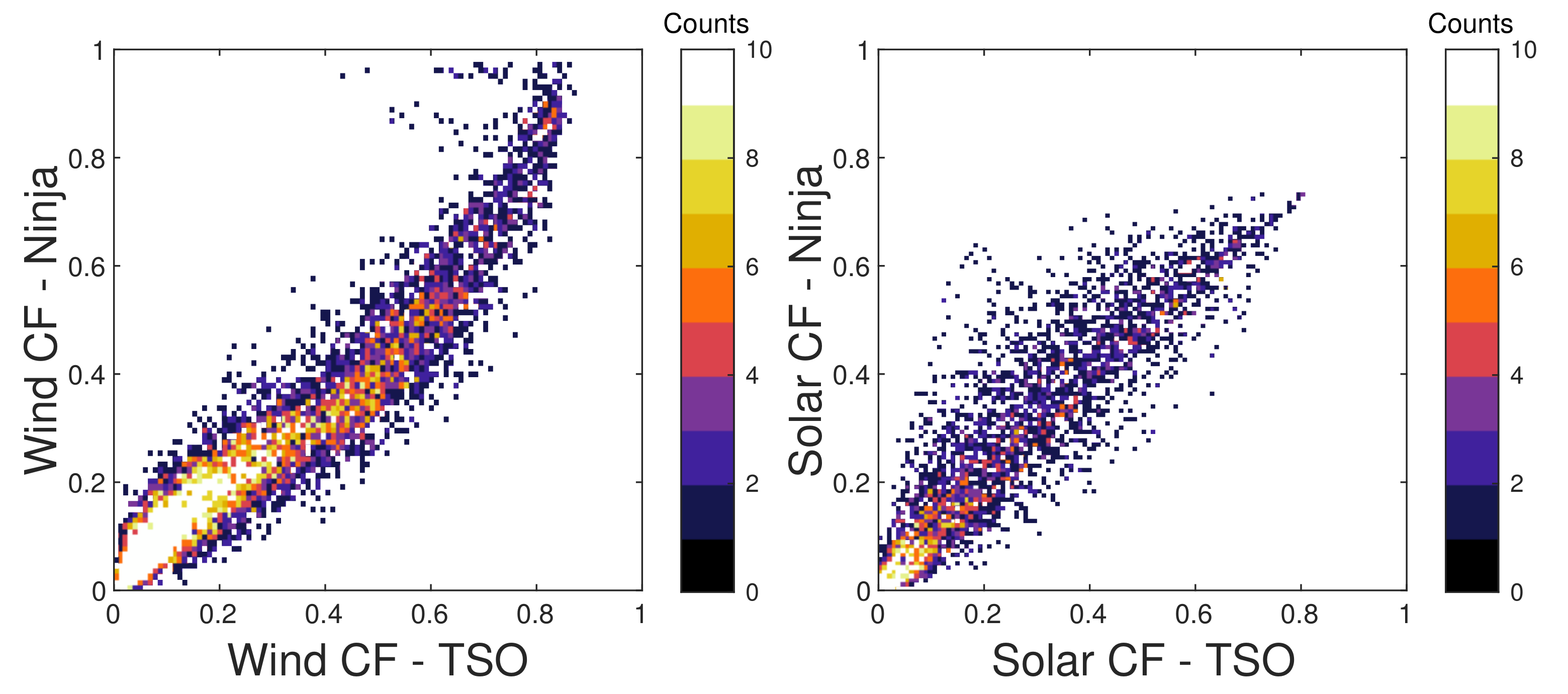
2.2. Validation of Simulated Power Production Data

In this section, we use measured power production data from the transmission system operators (TSOs) [55] to validate the capacity factors generated from the Renewables.ninja tool. Since the installed capacities used by the Renewables.ninja tool are constant based on the values as of December 2016, we used Belgian measured power production and installed capacity data for 2016 to validate the modeled data. It should be noted that the installed capacities of wind and solar power in Belgium were unchanged during 2016. Aggregated historical power production and installed capacity data are provided by the various TSOs (e.g., Elia for Belgium, TenneT, 50 Hertz, Amprion, and TransnetBW for Germany, and Energinet for Denmark). The Belgian power data have a sampling rate of 15 min, but we aggregated these to an hourly level to be consistent with the modeled capacity factor data. The wind and solar power production values have been normalized to their respective nominal capacities to obtain capacity factors. Scatter plots are shown in Figure 2 to compare the modeled wind and solar capacity factors with measured data from the TSO. Overall, the modeled capacities were reproduced quite well with Renewables.ninja data, though there was a small deviation at the higher end of the wind power capacity factor plot. Nonetheless, most of the values show a good correlation.

2.3. Reanalysis Data

To analyze the variability of meteorological conditions during Dunkelflaute events, the popular ERA5 reanalysis dataset was used (from ECMWF, the European Centre for Medium-Range Weather Forecasts [56]). ERA5 employs a horizontal grid size of 31 km and consists of hourly data. For this work, the same temporal coverage as provided by the Renewables.ninja tool (32 years, 1985–2016) was used. In our previous work, the ERA5 dataset has been shown to rather accurately characterize Dunkelflaute events [16], including reproducing vertical profiles and time series of various meteorological variables. In the present study, we utilized air pressure at mean sea level, cloud base height, and low cloud cover from the ERA5 dataset.

3. Characteristics of Wind and Solar Power Generation during Dunkelflaute

Taking Germany, Norway, and the UK as examples, Figure 3 shows the annual frequency of Dunkelflaute events defined using percentage capacity factor and time duration thresholds. In this figure, the capacity factor (CF) is defined as the fraction of wind and solar photovoltaic (PV) power production normalized by the respective installed capacity of wind and PV generation, where the fractions are the same for each. For example, a CF threshold value of 10% implies a capacity factor threshold of 10% for wind and 10% for PV. The number of Dunkelflaute events per year is noticeably decreased by reducing the capacity factor threshold or increasing the length of duration, since both conditions provide a more rigorous test for what constitutes a Dunkelflaute event.

For example, there are approximately 5–10 cases that are longer than one day each year in Germany for a threshold of 20% of capacity, with the most persistent events lasting for 4–5 days. These types of long-lasting Dunkelflaute events can challenge the grid operator when balancing supply and demand and may require the procurement of power from neighboring countries at a relatively high market price. In contrast, for a capacity threshold of 10%, there are hardly any cases lasting longer than two days, since one long-lasting event can be split into several shorter cases once there are a few samples having capacity factors larger than 10%.

When only considering prolonged periods of low wind power generation in Great Britain [8] (i.e., not accounting for PV generation), there are about 5–6 low wind production cases annually using a 5% CF threshold and persistence of longer than one day. Since the definition of a Dunkelflaute event includes both low wind and solar power production, the results in Figure 3 show a lower frequency of occurrence than that seen in [8]. It can also be seen that the number of events tagged as Dunkelflaute events does not vary much for the three different countries.

For the remainder of this paper, we have chosen to classify an event as a Dunkelflaute event if wind and solar CFs both fall below a specific threshold of 20% during a particular 60 min period, which means both wind and PV power production being lower than 20% of their respective capacities. It should be noted that although it can be expected that there is no or little solar power production after sunset and before sunrise, calm nighttime conditions are of significance from the point of view of system balancing, and therefore are included in this climatological analysis.

Figure 4 shows the frequency distribution of the length of events classified as Dunkelflaute for Belgium, Germany, and Denmark comparing modeled data from Renewables.ninja and the actual power production data from the TSOs. The frequency peaks at a duration between 12 and 24 h with a similar distribution for the three countries. There is good agreement between the two data sources, although there is an overestimation of the peak frequency for Germany using the Renewables.ninja data.

Figure 5 shows the average monthly hours of Dunkelflaute events for the eleven countries based on the Renewables.ninja data. We included only those events lasting for more than one day and plotted the total number of hours per month. As seen in the left panel of Figure 5, there is clearly a common distribution of the annual cycle of Dunkelflaute events for the different countries. Notably, almost all of the Dunkelflaute events lasting more than one day are predominantly present during the extended winter period (October–February). In fact, the occurrence of Dunkelflaute events mainly peaks in November, December, and January, during each of which there are 50–100 h of such events per year. One exception is in Sweden, with a larger magnitude of more than 150 h for the three months. The overall distribution is similar when using the measured (TSO) data in Belgium, Germany, and Denmark for 2015–2018 (refer to the right panel of Figure 5), though we can see a relatively larger magnitude of Dunkelflaute hours in January for the 4-year actual production data.

4. Meteorological Drivers

Dunkelflaute is shown to be associated with near-calm and stratus and/or stratocumulus-covered conditions driven by a high-pressure system [16]. We used hourly values of mean sea level pressure and cloud cover data from ERA5 for the Dunkelflaute periods during 1985–2016 to investigate how periods of Dunkelflaute are correlated with these variables. Spatial anomaly maps were created and averaged for those periods when Dunkelflaute events were prevalent. These Dunkelflaute periods were identified using the Renewable.ninja tool, as described before. Taking four representative countries of Denmark, Poland, Sweden, and the UK as examples, we analyzed the pressure and cloud cover maps to determine the weather factors giving rise to Dunkelflaute events for these countries.

4.1. Pressure

During Dunkelflaute periods (see top row of Figure 6), an extensive high-pressure system is clearly prevalent. The specific location, size, and magnitude of the system vary for individual events and countries. For example, during periods of Dunkelflaute in Denmark (top row, first column), Poland, and Sweden (top row, second and third columns, respectively), pressure in the Scandinavian area and Central Europe is higher than in the surrounding areas respectively, while for the UK (top row, fourth column), a high-pressure center is located over most of the North Sea area. Overall, the extended high surface pressure area developed over the four countries shows a slack pressure gradient, leading to a much lower surface wind speed in the individual countries. This is likely to lead to much lower levels of wind power production over an extended area.

These results are in agreement with previous studies, that show that large-scale high-pressure systems influence local weather and can further negatively affect both available wind and solar power generation [12,39,45]. These studies showed that such high-pressure systems are not associated with clear skies, but instead thick and extensive cloud cover, which are very characteristic of Dunkelflaute events (i.e., anticyclonic gloom weather [57,58]). This will be discussed further in the next section. Amongst the various synoptic-scale weather phenomena which have been shown to strongly affect wind power generation in western Europe [36,59,60,61], blocking of high-pressure systems (and the absence of westerly airflow into Europe) can result in extended periods of low production and periods of Dunkelflaute [36,37,38,39].

4.2. Cloud

Overcast sky with extensive low cloud cover is very characteristic of anticyclonic gloom weather. As seen in the maps of the mean cloud base height (CBH), when a Dunkelflaute event occurs, the height drops below 600 or even 400 m in the North and Baltic Sea areas and adjacent countries (second row of Figure 6). The third row of Figure 6 shows maps of the CBH anomaly calculated by subtracting the overall monthly mean CBH values from the mean values observed during periods of Dunkelflaute. Extensive areas of negative CBH anomaly (i.e., reduced CBH) are clearly seen over the four countries during periods of Dunkelflaute, with values of between approximately −500 and −100 m (third row of Figure 6).

Low-level cloud is an important element that strongly influences radiative features and local weather [62,63,64]. Over the North Sea, the low-level cloud is predominantly comprised of stratus, stratocumulus, and fog [65], consistent with the cloud cover types observed during anticyclonic gloom [16]. Several studies [66,67,68,69] have shown that synoptic conditions in the North Sea area frequently give rise to extensive stratocumulus clouds. For example, stratocumulus over the North Sea with a cloud top at 800 m and base at 400 m was observed by Nicholls [68], driven by a near stationary anticyclone located west of Ireland. Moderate winds with little shear were observed, which is also the case for nocturnal stratocumulus over the UK [66,67,69]. CBH for another five cases observed in the stratocumulus-topped boundary layer in the North Sea by Nicholls and Leighton [69] were all lower than or almost equal to 1000 m.

The high albedo of these low stratocumulus clouds can considerably reduce the incoming radiative flux at the surface. As described in [63,70,71,72], there is approximately a 40–50% reduction of surface solar radiation during the presence of stratus or stratocumulus clouds in comparison with cloud-free regions. The combination of lower than normal solar radiation over the regions of interest and shorter day lengths in winter (during which most Dunkelflaute events occur) indicates that total daily energy production from solar farms will be limited during periods of extensive stratocumulus. Furthermore, it should be noted that the occurrence of stratocumulus clouds mentioned above is associated with high-pressure systems, especially over the sea [63,69,70]. This is consistent with the observations in the previous section based on the top row of Figure 6.

Extensive coverage of low clouds (lower than approximately 2 km) also plays an important role in surface weather on the synoptic scale. The fourth row of Figure 6 suggests that low cloud cover (LCC) averaged for Dunkelflaute periods is around 0.7–0.9, which is significantly higher than the monthly mean LCC. This can be seen in the anomaly maps in the fifth row of Figure 6, where the mean overall LCC is subtracted from the mean LCC during Dunkelflaute events. Warren et al. [65] also found that LCC is about 0.7 when stratocumulus clouds occur over the North Sea. Positive anomaly values of LCC of around 0.1 to 0.3 are clear in the bottom row of Figure 6 for Dunkelflaute events occurring in Denmark, Poland, Sweden, and the UK.

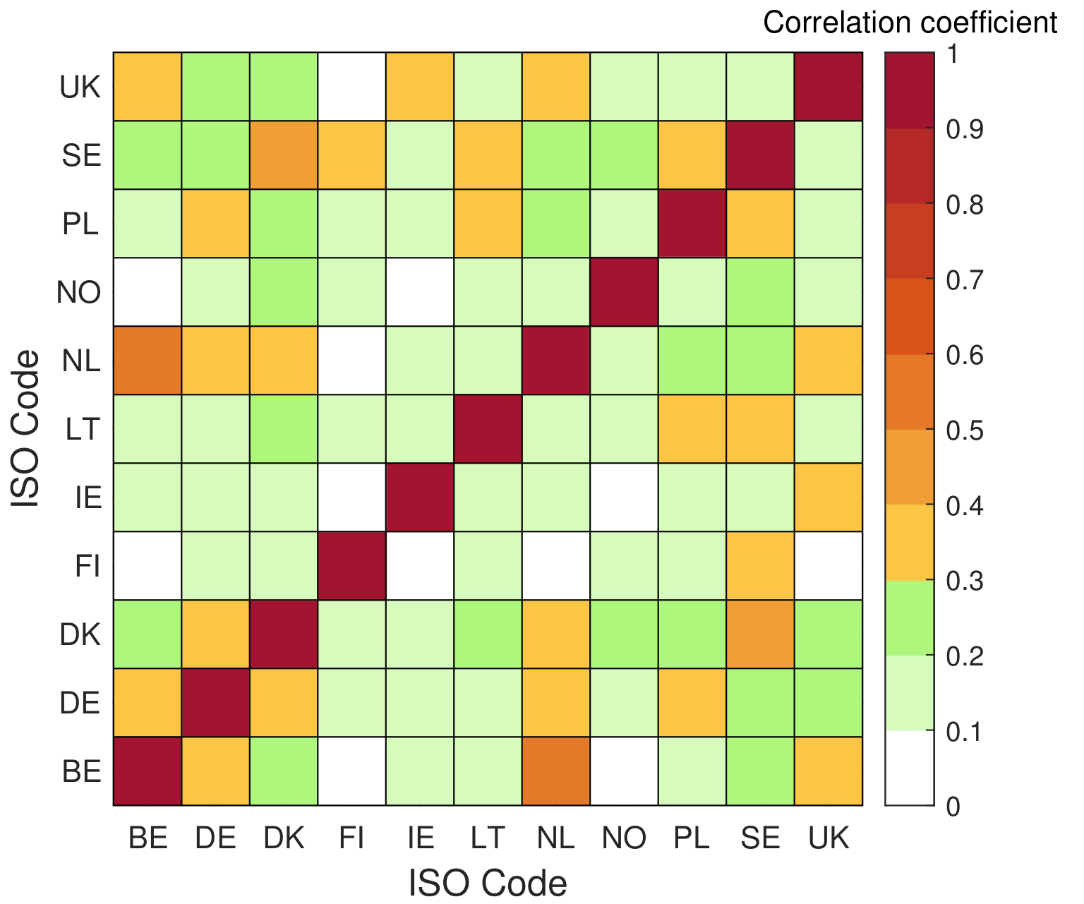
5. Spatial Correlation and Grid Connection

In this section, we quantify the spatial correlation of Dunkelflaute occurrences in eleven different European countries bordering the North and Baltic Sea areas. We used a binary flag (0 or 1) to represent non-Dunkelflaute and Dunkelflaute events (lasting more than one day) respectively, in individual countries, and calculated the Pearson correlation coefficient between each pair of the eleven countries. Although this metric is normally used for real numbers, it is also suitable for binary variables [73].

As shown in Figure 7, the correlation coefficients for Dunkelflaute events occurring in neighboring countries are about 0.3–0.4, with a peak magnitude of 0.5–0.6 for the Netherlands and Belgium, and Denmark and Sweden. This suggests that Dunkelflaute events can happen simultaneously over a relatively large area covering several countries. On the other hand, it is clear that Dunkelflaute periods are less correlated for those countries relatively far away from each other. Taking the UK as an example, when Dunkelflaute occurs there, there is a considerably lower probability of simultaneous Dunkelflaute occurrence in the Northern and central parts of Europe, such as in Finland and Poland.

From Figure 7, we can conclude that Dunkelflaute events rarely occur simultaneously in all eleven countries considered. Several multi-national power grid schemes have been proposed in Europe to benefit from integrated systems, such as the North Sea Offshore Grid project, which is expected to connect offshore renewable energy resources around the North Sea area [5], and the Baltic Energy Market Interconnection Plan, linking nine countries surrounding the Baltic Sea [50]. Therefore, it is interesting to consider what benefit can be gained from an interconnected European system of the eleven countries of interest studied here regarding the occurrence of Dunkelflaute events.

Figure 8 shows the reduction in the frequency of Dunkelflaute events (duration of longer than one day) for the eleven individual countries compared to an interconnected system where the wind and PV generation are pooled. The mean frequency of Dunkelflaute (marked as a black horizontal line) is decreased from 3–9% for the individual countries to approximately 3.5% when interconnected. Furthermore, the maximum frequency (marked as a blue ‘+’ symbol) is about 6.5% if power systems are interconnected, whereas individual countries can have frequency extremes of 6–14% of Dunkelflaute events. Pooling wind and PV generation through interconnection would seem to benefit most of the countries studied, especially Sweden and the Netherlands. The exceptions are Norway and the UK, where there seems to be only marginal or no benefit for these countries.

The right panel of Figure 8 provides further evidence for the benefits of interconnecting countries into a large power system. Taking four countries: Germany, Norway, Sweden, and the UK, as an example, we can see a reduction in the frequency of Dunkelflaute events for the larger interconnected power system, especially for those events that last for several consecutive days.

As illustrative examples, we used two Dunkelflaute events to quantify the benefits that can be gained through the interconnection into a larger power system of eleven countries (see Figure 9). The Dunkelflaute periods are marked as shaded gray regions under the curves. The first event occurred almost simultaneously in Ireland and the UK during late November of 2007, as shown in the left panels of Figure 9. The underproduction of wind and solar power lasted for about three days, and the positive effects of an interconnected system are clearly shown by leveling the capacity factor for the entire system, especially the wind CF, and alleviating the impacts of the Dunkelflaute events in the two countries. The second Dunkelflaute event is depicted in the right panel of Figure 9. During the early part of November 2013, Denmark and Sweden experienced Dunkelflaute episodes. If operational, the interconnected system (labelled as ’All’) would have been able to increase the capacity factors of both wind and solar and circumvent the Dunkelflaute events. In the literature, other benefits of interconnected systems have been demonstrated, including a relative reduction in wind power variability [74,75,76] and a reduction in flexibility requirements [11,77].

6. Concluding Remarks

A climatological analysis of Dunkelflaute events was carried out for eleven countries bordering the North and Baltic Sea areas. Utilizing a wind and PV capacity factor threshold of 20%, we can conclude that substantial periods of Dunkelflaute lasting for at least a day occur each year. For example, there were approximately 2–10 events (duration of longer than one day) each year in three of the exampled countries, Germany, Norway, and the UK, and similar frequencies were also found in the other eight countries. Notably, there were a few cases lasting three or even five days. The largest frequency of Dunkelflaute events was seen in November, December, and January.

These events were shown to be typically characterized by near stationary large-scale high-pressure systems and extensive low cloud coverage, with a lower than average cloud base height. This confirms the association of the Dunkelflaute events and blocked regimes arising from the extensive high pressure, which can obstruct the westerly airflow into Europe and further result in the underproduction of wind energy in the neighboring countries. Furthermore, the occurrence of expansive low-level clouds was shown to be another characteristic of Dunkelflaute events, which further corroborates the previous finding that the high-pressure ridges between frontal systems are associated with the occurrence of stratocumulus clouds in mid-latitudes [63,70]. Due to the relatively low solar radiation and shorter day lengths in winter (during which most Dunkelflaute events occur), the limited solar energy production during the events can thus be well-explained.

Lastly, it was found that the correlation coefficients of Dunkelflaute events for neighboring countries were moderate (approximately 0.3–0.4). Simple analysis revealed that an interconnected power system where wind and PV generation are pooled can decrease the occurrence of Dunkelflaute events considerably. Our findings, albeit preliminary, can be of importance for reducing the risk of black-outs or the necessity for backup energy demands and costs to maintain system stability, especially for high renewable penetration in the near future.

References

1. Matthias, B.; Andreas, G.; Patrick, G. European Energy Transition 2030: The Big Picture. Ten Priorities for the Next European Commission to Meet the EU’s 2030 Targets and Accelerate towards 2050; 153/01-I-2019/EN; Agora Energiewende: Berlin, Germany, 2019; pp. 1–103. [Google Scholar]
2. European Commission. Report from the Commission to the European Parliament, the Council, the European Economic and Social Committee and the Committee of the Regions on the Implementation of EU Macro-Regional Strategies; COM_2019_0021_FIN; European Commission: Brussels, Belgium, 2019; pp. 1–12. [Google Scholar]
3. European Commission. Energy Roadmap 2050; 978-92-79-21798-2; Publications Office of the European Union: Brussels, Belgium, 2012; pp. 1–20. [Google Scholar]
4. Müller, M.; Haesen, E.; Ramaekers, L.; Verkaik, N. Translate COP21—2045 Outlook and Implications for Offshore Wind in the North Seas; ESMNL17412; Ecofys: Utrecht, The Netherlands, 2017; pp. 1–21. [Google Scholar]
5. European Commission. Political Declaration on Energy Cooperation between the North Seas Countries; European Commission: Brussels, Belgium, 2016; pp. 1–7. [Google Scholar]
6. Wind Europe. Boosting Offshore Wind Energy in the Baltic Sea; Wind Europe: Brussels, Belgium, 2019; pp. 1–11. [Google Scholar]
7. Bloomfield, H.C.; Brayshaw, D.J.; Shaffrey, L.C.; Coker, P.J.; Thornton, H.E. Quantifying the increasing sensitivity of power systems to climate variability. Environ. Res. Lett. 2016, 11, 124025. [Google Scholar] [CrossRef]
8. Cannon, D.J.; Brayshaw, D.J.; Methven, J.; Coker, P.J.; Lenaghan, D. Using reanalysis data to quantify extreme wind power generation statistics: A 33 year case study in Great Britain. Renew. Energy 2015, 75, 767–778. [Google Scholar] [CrossRef] [Green Version]
9. Santos-Alamillos, F.J.; Pozo-Vázquez, D.; Ruiz-Arias, J.A.; Lara-Fanego, V.; Tovar-Pescador, J. Analysis of spatiotemporal balancing between wind and solar energy resources in the southern Iberian Peninsula. J. Appl. Meteorol. Climatol. 2012, 51, 2005–2024. [Google Scholar] [CrossRef]
10. Bett, P.E.; Thornton, H.E.; Clark, R.T. European wind variability over 140 yr. Adv. Sci. Res. 2013, 10, 51–58. [Google Scholar] [CrossRef] [Green Version]
11. Huber, M.; Dimkova, D.; Hamacher, T. Integration of wind and solar power in Europe: Assessment of flexibility requirements. Energy 2014, 69, 236–246. [Google Scholar] [CrossRef] [Green Version]
12. van der Wiel, K.; Stoop, L.P.; Van Zuijlen, B.R.H.; Blackport, R.; Van den Broek, M.A.; Selten, F.M. Meteorological conditions leading to extreme low variable renewable energy production and extreme high energy shortfall. Renew. Sustain. Energy Rev. 2019, 11, 261–275. [Google Scholar] [CrossRef]
13. Oswald, J.; Raine, M.; Ashraf-Ball, H. Will British weather provide reliable electricity? Energy Policy 2008, 36, 3212–3225. [Google Scholar] [CrossRef]
14. Zachary, S.; Dent, C.J. Probability theory of capacity value of additional generation. Proc. Inst. Mech. Eng. Part O J. Risk Reliab. 2012, 226, 33–43. [Google Scholar] [CrossRef] [Green Version]
15. Harrison, G.P.; Hawkins, S.L.; Eager, D.; Cradden, L.C. Capacity value of offshore wind in Great Britain. Proc. Inst. Mech. Eng. Part O J. Risk Reliab. 2015, 229, 360–372. [Google Scholar] [CrossRef] [Green Version]
16. Li, B.; Basu, S.; Watson, S.J.; Russchenberg, H.W. Mesoscale modeling of a “Dunkelflaute” event. Wind Energy 2021, 24, 5–23. [Google Scholar] [CrossRef]
17. Li, B.; Basu, S.; Watson, S.J.; Russchenberg, H.W. Quantifying the Predictability of a ‘Dunkelflaute’ Event by Utilizing a Mesoscale Model. J. Phys. Conf. Ser. 2020, 1618, 062042. [Google Scholar] [CrossRef]
18. NOS. Netbeheerder Moest Groot Inkopen om Stroomtekort op te Vangen. Available online: https://nos.nl/artikel/2229787-netbeheerder-moest-groot-inkopen-om-stroomtekort-op-te-vangen.html (accessed on 4 November 2020).
19. NRC. Netbeheerder Tennet Wendt Landelijk Stroomtekort af. Available online: https://www.nrc.nl/nieuws/2018/04/30/landelijk-stroomtekort-afgewend-door-netbeheerder-tennet-a1601355 (accessed on 4 November 2020).
20. Meinke-Hubeny, F.; de Oliveira, L.P.N.; Duerinck, J.; Lodewijks, P.; Belmans, R. Energy Transition in Belgium—Choices and Costs; EnergyVille in Opdracht van Febeliec: Genk, Belgium, 2017. [Google Scholar]
21. Elia. Electricity Scenarios for Belgium towards 2050, Elia’s Quantified Study on the Energy Transition in 2030 and 2040; Elia: Brussels, Belgium, 2017; pp. 1–150. [Google Scholar]
22. Wetzel, D. Die “Dunkelflaut”’ Bringt Deutschlands Stromversorgung ans Limit. Available online: https://www.welt.de/wirtschaft/article161831272/Die-Dunkelflaute-bringt-Deutschlands-Stromversorgung-ans-Limit.html (accessed on 4 November 2020).
23. Schultz, S. Ist der Winter Wirklich zu Düster für den Ökostrom? Available online: https://www.spiegel.de/wirtschaft/soziales/oekostrom-knapp-panikmache-mit-der-dunkelflaute-a-1133450.html (accessed on 4 November 2020).
24. Pfenninger, S. Dealing with multiple decades of hourly wind and PV time series in energy models: A comparison of methods to reduce time resolution and the planning implications of inter-annual variability. Appl. Energy 2017, 197, 1–13. [Google Scholar] [CrossRef]
25. Staffell, I.; Pfenninger, S. The increasing impact of weather on electricity supply and demand. Energy 2018, 145, 65–78. [Google Scholar] [CrossRef]
26. Widén, J. Correlations between large-scale solar and wind power in a future scenario for Sweden. IEEE Trans. Sustain. Energy 2011, 2, 177–184. [Google Scholar] [CrossRef]
27. Grünewald, P.; Cockerill, T.; Contestabile, M.; Pearson, P. The role of large scale storage in a GB low carbon energy future: Issues and policy challenges. Energy Policy 2011, 39, 4807–4815. [Google Scholar] [CrossRef]
28. Schroeder, A.; Oei, P.Y.; Sander, A.; Hankel, L.; Laurisch, L.C. The integration of renewable energies into the German transmission grid—A scenario comparison. Energy Policy 2013, 61, 140–150. [Google Scholar] [CrossRef]
29. Heide, D.; Von Bremen, L.; Greiner, M.; Hoffmann, C.; Speckmann, M.; Bofinger, S. Seasonal optimal mix of wind and solar power in a future, highly renewable Europe. Renew. Energy 2010, 35, 2483–2489. [Google Scholar] [CrossRef]
30. Santos-Alamillos, F.J.; Pozo-Vázquez, D.; Ruiz-Arias, J.A.; Von Bremen, L.; Tovar-Pescador, J. Combining wind farms with concentrating solar plants to provide stable renewable power. Renew. Energy 2015, 76, 539–550. [Google Scholar] [CrossRef]
31. Pfenninger, S.; Keirstead, J. Renewables, nuclear, or fossil fuels? Scenarios for Great Britain’s power system considering costs, emissions and energy security. Appl. Energy 2015, 152, 83–93. [Google Scholar] [CrossRef] [Green Version]
32. Buttler, A.; Dinkel, F.; Franz, S.; Spliethoff, H. Variability of wind and solar power—An assessment of the current situation in the European Union based on the year 2014. Energy 2016, 106, 147–161. [Google Scholar] [CrossRef]
33. Plaut, G.; Simonnet, E. Large-scale circulation classification, weather regimes, and local climate over France, the Alps and Western Europe. Clim. Res. 2001, 17, 303–324. [Google Scholar] [CrossRef]
34. Yiou, P.; Nogaj, M. Extreme climatic events and weather regimes over the North Atlantic: When and where? Geophys. Res. Lett. 2004, 31, L07202. [Google Scholar] [CrossRef]
35. Donat, M.G.; Leckebusch, G.C.; Pinto, J.G.; Ulbrich, U. Examination of wind storms over Central Europe with respect to circulation weather types and NAO phases. Int. J. Climatol. 2010, 30, 1289–1300. [Google Scholar] [CrossRef] [Green Version]
36. Zubiate, L.; McDermott, F.; Sweeney, C.; O’Malley, M. Spatial variability in winter NAO–wind speed relationships in western Europe linked to concomitant states of the East Atlantic and Scandinavian patterns. Q. J. R. Meteorol. Soc. 2017, 143, 552–562. [Google Scholar] [CrossRef] [Green Version]
37. Thornton, H.E.; Scaife, A.A.; Hoskins, B.J.; Brayshaw, D.J. The relationship between wind power, electricity demand and winter weather patterns in Great Britain. Environ. Res. Lett. 2017, 12, 064017. [Google Scholar] [CrossRef]
38. Grams, C.M.; Beerli, R.; Pfenninger, S.; Staffell, I.; Wernli, H. Balancing Europe’s wind-power output through spatial deployment informed by weather regimes. Nat. Clim. Chang. 2017, 7, 557–562. [Google Scholar] [CrossRef] [PubMed] [Green Version]
39. Bloomfield, H.C.; Brayshaw, D.J.; Shaffrey, L.C.; Coker, P.J.; Thornton, H.E. The changing sensitivity of power systems to meteorological drivers: A case study of Great Britain. Environ. Res. Lett. 2018, 13, 054028. [Google Scholar] [CrossRef]
40. Pozo-Vázquez, D.; Tovar-Pescador, J.; Gámiz-Fortis, S.R.; Esteban-Parra, M.J.; Castro-Díez, Y. NAO and solar radiation variability in the European North Atlantic region. Geophys. Res. Lett. 2004, 31, 1–4. [Google Scholar] [CrossRef]
41. Dutton, E.G.; Farhadi, A.; Stone, R.S.; Long, C.N.; Nelson, D.W. Long-term variations in the occurrence and effective solar transmission of clouds as determined from surface-based total irradiance observations. J. Geophys. Res. 2004, 109, D03204. [Google Scholar] [CrossRef]
42. Dutton, E.G.; Nelson, D.W.; Stone, R.S.; Longenecker, D.; Carbaugh, G.; Harris, J.M.; Wendell, J. Decadal variations in surface solar irradiance as observed in a globally remote network. J. Geophys. Res. 2006, 111, D19101. [Google Scholar] [CrossRef] [Green Version]
43. Sanchez-Lorenzo, A.; Calbó, J.; Martin-Vide, J. Spatial and temporal trends in sunshine duration over Western Europe (1938–2004). J. Clim. 2008, 21, 6089–6098. [Google Scholar] [CrossRef]
44. Chiacchio, M.; Wild, M. Influence of NAO and clouds on long-term seasonal variations of surface solar radiation in Europe. J. Geophys. Res. 2010, 115, D00D22. [Google Scholar]
45. van der Wiel, K.; Bloomfield, H.C.; Lee, R.W.; Stoop, L.P.; Blackport, R.; Screen, J.A.; Selten, F.M. The influence of weather regimes on European renewable energy production and demand. Environ. Res. Lett. 2019, 14, 094010. [Google Scholar] [CrossRef]
46. Watts, A. Weather Wise: Reading Weather Signs; Adlard Coles, Bloomsbury Publishing: London, UK, 2013. [Google Scholar]
47. Douglas, C.K.M. Clouds as seen from an aeroplane. Q. J. R. Meteorol. Soc. 1920, 46, 233–242. [Google Scholar] [CrossRef]
48. Staffell, I.; Pfenninger, S. Using bias-corrected reanalysis to simulate current and future wind power output. Energy 2016, 114, 1224–1239. [Google Scholar] [CrossRef] [Green Version]
49. Pfenninger, S.; Staffell, I. Long-term patterns of European PV output using 30 years of validated hourly reanalysis and satellite data. Energy 2016, 114, 1251–1265. [Google Scholar] [CrossRef] [Green Version]
50. Energy and Climate Change Committee. A European Supergrid; The Stationery Office Limited: London, UK, 2011. [Google Scholar]
51. IRENA. Renewable Energy Capacity Statistics 2015; IRENA: Abu Dhabi, United Arab Emirates, 2015. [Google Scholar]
52. IRENA. Renewable Capacity Statistics 2021; IRENA: Abu Dhabi, United Arab Emirates, 2021. [Google Scholar]
53. Lu, X.; McElroy, M.B.; Kiviluoma, J. Global potential for wind-generated electricity. Proc. Natl. Acad. Sci. USA 2009, 106, 10933–10938. [Google Scholar] [CrossRef] [Green Version]
54. McKenna, R.; Hollnaicher, S.; Leye, P.O.v.d.; Fichtner, W. Cost-potentials for large onshore wind turbines in Europe. Energy 2015, 83, 217–229. [Google Scholar] [CrossRef]
55. Available online: https://www.entsoe.eu/data/ (accessed on 8 October 2021).
56. Hersbach, H.; Bell, B.; Berrisford, P.; Hirahara, S.; Horányi, A.; Muñoz-Sabater, J.; Nicolas, J.; Peubey, C.; Radu, R.; Schepers, D.; et al. The ERA5 global reanalysis. Q. J. R. Meteorol. Soc. 2020, 146, 1999–2049. [Google Scholar] [CrossRef]
57. Allaby, M. Encyclopedia of Weather and Climate; Facts on File: New York, NY, USA, 2007. [Google Scholar]
58. Weller, J.; Thornes, J.E. An investigation of winter nocturnal air and road surface temperature variation in the West Midlands, UK under different synoptic conditions. Meteorol. Appl. 2001, 8, 461–474. [Google Scholar] [CrossRef]
59. Brayshaw, D.J.; Troccoli, A.; Fordham, R.; Methven, J. The impact of large scale atmospheric circulation patterns on wind power generation and its potential predictability: A case study over the UK. Renew. Energy 2011, 36, 2087–2096. [Google Scholar] [CrossRef]
60. Ely, C.R.; Brayshaw, D.J.; Methven, J.; Cox, J.; Pearce, O. Implications of the North Atlantic Oscillation for a UK–Norway renewable power system. Energy Policy 2013, 62, 1420–1427. [Google Scholar] [CrossRef] [Green Version]
61. Burningham, H.; French, J. Is the NAO winter index a reliable proxy for wind climate and storminess in northwest Europe? Int. J. Climatol. 2013, 33, 2036–2049. [Google Scholar] [CrossRef] [Green Version]
62. Slingo, A.; Slingo, J.M. The response of a general circulation model to cloud longwave radiative forcing. I: Introduction and initial experiments. Q. J. R. Meteorol. Soc. 1988, 114, 1027–1062. [Google Scholar] [CrossRef]
63. Driedonks, A.G.M.; Duynkerke, P.G. Current problems in the stratocumulus-topped atmospheric boundary layer. Bound.-Layer Meteorol. 1989, 46, 275–303. [Google Scholar] [CrossRef]
64. Viúdez-Mora, A.; Costa-Surós, M.; Calbó, J.; González, J.A. Modeling atmospheric longwave radiation at the surface during overcast skies: The role of cloud base height. J. Geophys. Res. Atmos. 2015, 120, 199–214. [Google Scholar] [CrossRef] [Green Version]
65. Warren, G.; Hahn, J.; London, J.; Chervin, M.; Jenne, L. Global Distribution of Total Cloud Cover and Cloud Type Amounts over Land; National Center for Atmospheric Research: Boulder, CO, USA, 1986. [Google Scholar]
66. Caughey, S.J.; Crease, B.A.; Roach, W.T. A field study of nocturnal stratocumulus II Turbulence structure and entrainment. Q. J. R. Meteorol. Soc. 1982, 108, 125–144. [Google Scholar] [CrossRef]
67. Slingo, A.; Brown, R.; Wrench, C.L. A field study of nocturnal stratocumulus; III. High resolution radiative and microphysical observations. Q. J. R. Meteorol. Soc. 1982, 108, 145–165. [Google Scholar] [CrossRef]
68. Nicholls, S. The dynamics of stratocumulus: Aircraft observations and comparisons with a mixed layer model. Q. J. R. Meteorol. Soc. 1984, 110, 783–820. [Google Scholar] [CrossRef]
69. Nicholls, S.; Leighton, J. An observational study of the structure of stratiform cloud sheets: Part I. Structure. Q. J. R. Meteorol. Soc. 1986, 112, 431–460. [Google Scholar] [CrossRef]
70. Duynkerke, P.G.; Driedonks, A.G.M. A Model for the Turbulent Structure of the Stratocumulus–Topped Atmospheric Boundary Layer. J. Atmos. Sci. 1987, 44, 43–64. [Google Scholar] [CrossRef] [Green Version]
71. Hartmann, D.L.; Ockert-Bell, M.E.; Michelsen, M.L. The effect of cloud type on Earth’s energy balance: Global analysis. J. Clim. 1992, 5, 1281–1304. [Google Scholar] [CrossRef] [Green Version]
72. Wood, R. Stratocumulus clouds. Mon. Weather Rev. 2012, 140, 2373–2423. [Google Scholar] [CrossRef]
73. Zhang, B.; Srihari, S.N. Properties of binary vector dissimilarity measures. Proc. JCIS Int. Conf. Comput. Vis. Pattern Recognit. Image Process. 2003, 1, 1–4. [Google Scholar]
74. Kempton, W.; Pimenta, F.M.; Veron, D.E.; Colle, B.A. Electric power from offshore wind via synoptic-scale interconnection. Proc. Natl. Acad. Sci. USA 2010, 107, 7240–7245. [Google Scholar] [CrossRef] [Green Version]
75. Jacobson, M.Z.; Delucchi, M.A. Providing all global energy with wind, water, and solar power, Part I: Technologies, energy resources, quantities and areas of infrastructure, and materials. Energy Policy 2011, 39, 1154–1169. [Google Scholar] [CrossRef]
76. Holttinen, H.; Rissanen, S.; Larsen, X.; Løvholm, A.L. Wind and Load Variability in the Nordic Countries; VTT Technical Research Centre of Finland: Espoo, Finland, 2013. [Google Scholar]
77. Becker, S.; Rodriguez, R.A.; Andresen, G.B.; Schramm, S.; Greiner, M. Transmission grid extensions during the build-up of a fully renewable pan-European electricity supply. Energy 2014, 64, 1404–1418. [Google Scholar] [CrossRef] [Green Version]
Figure 1. The eleven countries studied in the research bordering the North and Baltic Sea areas. For each country, the wind and solar capacities (MW) for the year of 2020 are listed, respectively [52].
Energies 14 06508 g001
Figure 2. Bi-variate histograms of modeled and actual wind (left panel) and solar (right panel) power capacity factors (CF) for 2016 in Belgium.
Energies 14 06508 g002
Figure 3. The frequency of Dunkelflaute events for Germany (left panel), Norway (middle panel), and the UK (right panel) respectively, using different thresholds for capacity factor and time duration. The underlying data, spanning the years of 1985 to 2016, were generated by the Renewables.ninja tool.
Energies 14 06508 g003
Figure 4. Frequency distribution of modeled (ninja) and actual (TSO) Dunkelflaute durations for Belgium (left panel), Germany (middle panel), and Denmark (right panel). The modeled data, spanning the years of 1985 to 2016, were generated by the Renewables.ninja tool. Actual power production data from the TSOs are for the years 2015–2018.
Energies 14 06508 g004
Figure 5. The (left panel) shows the monthly variation of Dunkelflaute hours per year for eleven countries over the North Sea and Baltic Sea based on the Renewable.ninja data. The (right panel) is similar but using actual production data from the TSOs to identify Dunkelflaute in Belgium (BE), Germany (DE), and Denmark (DK) for 2015–2018. We only account for the Dunkelflaute events longer than one day.
Energies 14 06508 g005
Figure 6. Map of mean sea level pressure (MSLP, top row), cloud base height (CBH, second row), CBH anomaly (third row), low cloud cover (LCC, fourth row), and LCC anomaly (bottom row) during Dunkelflaute periods in Denmark (left column), Poland (middle-left column), Sweden (middle-right column), and the UK (right column), respectively. Anomaly maps were created by subtracting the monthly mean values from mean values when Dunkelflaute occurs.
Energies 14 06508 g006
Figure 7. Correlation coefficients of Dunkelflaute occurrences between eleven European countries.
Energies 14 06508 g007
Figure 8. (Left panel): frequency boxplot of Dunkelflaute events (longer than a day) for individual countries and where wind and PV generation are pooled in an interconnected system of eleven countries (labeled as ‘All’). (Right panel): frequency distribution of Dunkelflaute events for four representative countries (Germany (DE), Norway (NO), Sweden (SE), and the UK) and an interconnected system (labeled as ‘All’). The frequency for the interconnected system is given by gray bars, while the frequency for the four individual countries is shown in color as a deviation from the magnitude of the interconnected system.
Energies 14 06508 g008
Figure 9. Time series of wind capacity factor (top panel) and solar capacity (bottom panel) during two cases of Dunkelflaute, which occurred in Ireland (IE), the UK (left panel), Denmark (DK), and Sweden (SE, right panel), respectively. The wind and solar CF are shown for the individual countries and an interconnected system of eleven countries (labeled as ‘All’). The Dunkelflaute periods are demarcated by shaded gray regions. Different shades correspond to different countries.
Energies 14 06508 g009
Publisher’s Note: MDPI stays neutral with regard to jurisdictional claims in published maps and institutional affiliations.