Abstract
This paper proposes the computation and assessment of optimal tilt and azimuth angles for a receiving surface, using a mathematical model developed at the University of Tomsk, Russia. The model was validated and analyzed for the Nuevo León State, Northeast Mexico, utilizing a set of metrics, comparing against satellite data from NASA. A point of interest in the city of Monterrey was analyzed to identify orientation patterns throughout the year for an optimal solar energy gathering. The aim is providing the best orientation tilt angles for photovoltaic or solar thermal panels without tracking systems. In addition, this analysis is proposed as a tool to achieve optimal performance in sustainable urban development in the region. Based on the findings, a set of optimal tilt and azimuth surface angles are proposed for the analyzed coordinates. The aim is to identify the optimal performance to obtain the maximum solar irradiation possible over the year for solar projects in the region. The results show that the model can be used as a tool to accelerate decision making in the design of solar harvesting surfaces and allows the design of discrete tracking systems with an increase in solar energy harvesting above 5% annually.
1. Introduction
Renewable energy sources are essential to reduce greenhouse gases (GHG) and for sustainable development. One of the main sources of renewable energy due to its accessibility is solar radiation. The energy and land usage in several Italian provinces were studied to analyze whether solar energy is the optimal renewable energy source to reach the 2030 climate policies in Europe. It was concluded that solar energy is the cheapest renewable energy source with the largest potential in the latitude of Italy [1]. This form of energy can be harnessed by photovoltaic (PV) panels that work with semiconductors that release electrons when in contact with solar radiation [2]. This process can be both used for industrial and domestic purposes. Mexico has the potential capacity to develop renewable technologies and produce 1172 gigawatts, stating that solar power is the best technology in every scenario considered [3]. A great area of solar potential is the northeast, where Nuevo León state is located. From an economical perspective, an advantage of Nuevo León is the geographical location that opens the possibility of forming an integrated North American energy market [3,4].
In recent years, mathematical models of solar radiation have been refined because they can significantly reduce the price and time of development of solar energy projects [5]. In this regard, several tools have been tested for their efficiency, such as in [6], where 23 software packages and 4 mobile apps regarding photovoltaic systems were analyzed; they found that none of the tools reviewed met every benchmark set of design and management purposes. In order to improve these calculations, a system of eight different factors that improve decision making during PV projects was proposed. The proposition of the system is that, for future work, researchers should focus on working on these factors, such as optimization of the PV layout design, instead of building a general design software for PV arrays.
An extensively used approach to estimating solar resources is the utilization of satellites. According to [7], a mathematical model, supported by the NASA SSE database, was applied to predict the characteristics of solar radiation for any latitude and longitude in Russia. Recently, reference [4] found that the model is a good estimation of solar resources available and depends only on the geographical location and data available in the satellite NASA SSE database. This fact allows the model to be independent of meteorological stations or physical limitations and provides better coverage of the region [4].
Studies made in Libya by the Sebelas Maret University to compute the maximum solar radiation were conducted, using a mathematical model to determine the optimal orientation and positioning of a solar panel [8]. Similar calculations were made in Tunisia [9], where they addressed the issue of computing the angle of PV panels. This was done as an alternative to solar tracking control systems. Furthermore, calculating the best tilt angle of the solar panels using mathematical modeling would make it easier to implement PV panels and ensure their maximum efficiency.
A mathematical model computed the optimal tilt and azimuth angle for a PV array in [10] for the city of Sharjah in the United Arab Emirates. The results showed a set of optimal angles for Sharjah, using the sensitivity analysis of design parameters of bi-facial solar PV technology. They studied the effects of albedo, tilt angle, and height from the ground against power gain correlations. The application of the findings served to increase the energy supply for the existent solar panels and to reduce the energy demand for cooling in the buildings where PV systems were installed. The optimization of the tilt angle in the PV systems had the highest effect during the winter in Punjab, Pakistan; this result can be especially useful since the days are shorter and more energy is required for lightning purposes [11].
In reference [8], a study to estimate solar radiation is presented. Three mathematical models were compared: the Caperdaou, the Liu and Jordan, and the R. Sun model. These were compared against the solar radiation received by a ground collector, and it was found that the Caperdaou model was the most suitable for the Algerian region.
In Mexico, the solarimetric network is currently managed by the Mexican National Weather Service (SMN). This network consists of several meteorological stations deployed all over the country, which measures several variables of weather, including solar radiation. The Mexican grid consists of two types of stations: automatic meteorological stations (EMAs) and synoptic meteorological stations (ESIMEs). EMAs are conformed by mechanical and electronic devices, such as sensors that monitor several meteorological variables. These stations have the following sensors: wind speed, direction of the wind, atmospheric pressure, temperature, relative humidity, solar radiation, and precipitation [12]. ESIMEs are a set of sensors that realizes measurements automatically from the previously mentioned meteorology variables [12]. Another difference between an EMA and an ESIME lies in the way the information is presented; in EMAs, a file is created every ten minutes with all the necessary variables. On the other hand, ESIMEs generate a synoptic message every three hours [12]. The Mexican grid counts with only 189 EMAs, and 84 ESIMEs all over Mexico [12]. In the state of Nuevo León, there are only three EMAs and one ESIME, as shown in Figure 1, where the state is highlighted; these are not enough to have a complete panoramic of the solar radiation in the state. Additionally, according to [13], more than half of the solar radiation sensors may not be correctly calibrated, leading to higher discrepancies in the station results when measuring the solar radiation. In the same study, it is stated that these measurements are not public and have a higher error than satellite readings, which is around 10%. Another study of solar radiation in Mexico analyzed the findings of the meteorological stations to validate their mathematical model, and found that only 33% of the stations in the Sonoran region in northwest Mexico met their selection criteria [4].
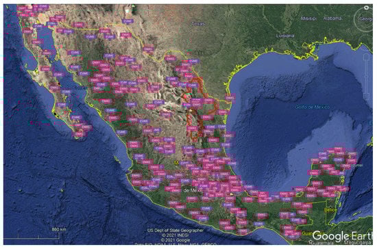
Figure 1.
Mexican meteorological grid. The state of Nuevo León is highlighted in red.
Due to the scarcity of local data concerning radiation analysis in Mexican geographical coordinates, in this study, some relevant contributions with respect to the irradiation calculations regarding the surface angle were made. These calculations were made for the city of Monterrey in Mexico to build a photovoltaic array. However, they can be extrapolated in order to analyze any coordinates in the world. The main objective of the current research is utilizing a mathematical model as a tool to identify and propose several setups for tilt and azimuth angles for solar collecting surfaces with no tracking systems and increase their energy harvesting throughout the year as close as possible to an optimal point. The idea is to save costs of tracking systems required by other technologies (such as full tracking, or partial tracking), which require sensors and mechanical systems, as well as increasing performance and production for future efficient solar systems (PV or solar thermal), which impact in the green development in the region.
The literature review indicates the importance of calculating the parameters of solar radiation acting on collecting surfaces as a way to identify the harvesting of the highest amount of solar energy possible during the year. This paper is aimed to calculate and assess the solar irradiation on a receiving surface at different tilt and azimuth angles to obtain the greatest amount of energy captured, utilizing a mathematical model as a tool with a data-driven approach based on the geospatial information retrieved.
This approach does not require weather stations, or a local sensing device deployed, avoiding the cost of equipment and maintenance. Besides this, the proposed approach can use databases which provides the albedo, the reflection index and the geographic coordinates. This makes the approach flexible and adaptable.
This study is organized as follows: Section 2 describes the data source used to compare the mathematical model. Section 3 presents the methodology, which describes the mathematical model and statistical methods used to validate and analyze the impact of different tilt and azimuth angles for a receiving surface. Section 4 consists of a report and discussion of the accuracy of the model and the effect of changing the surface angles previously mentioned in the methodology. Finally, Section 5 provides the conclusions and offers a brief mention of further research opportunities.
2. Data Sources
The present work used a resource to gather data related to solar radiation. The obtained information was later compared with the findings of the mathematical model in order to validate it. The resource was the database of NASA’s Surface Meteorology and Solar Energy (SSE). As stated in the introduction, the set of EMAs and ESIMEs is scarce (only four stations) and cannot be used to have a complete representation of the state of Nuevo León. Due to this, it was decided not to use the Mexican national weather service findings to validate the model.
The database of NASA’s Surface Meteorology and Solar Energy (SSE) contains information about solar measurements, such as surface albedo () and the clarity index () [14]. These two parameters represent the capacity of light reflection and the atmospheric effect on light for the analyzed zone. These are used as inputs for the mathematical model to calculate the solar irradiation.
Five geographic points were selected to cover a sufficiently representative area of the state of Nuevo León, where Colombia is at the north of the state, Linares at the center, El Grullo at the east, Monterrey at the west and Mier y Noriega at the south. Then, the average total solar irradiation per month was calculated from these specific geographic points and compared against the data from the NASA SSE database. Table 1 present the locations and geographic coordinates.

Table 1.
Geographical data for the selected municipalities.
3. Methodology
The methodology consisted of calculating solar irradiation based on a mathematical model proved for other geographical regions around the world. This model was applied to a specific point in the city of Monterrey as a case study. A comparison of different angles (tilt and orientation) of the receiving surface was utilized for the calculations. Then, statistical methods were used to compare the model against the values of solar irradiation at the ground level of the NASA database. It is worth mentioning that NASA only provides the solar irradiation that reaches a horizontal surface without tilt or azimuth surface angles; therefore, the NASA data source focuses only on horizontal surfaces (parallel to the ground) at different altitudes for its data of solar irradiation. On the other hand, the model used in this research work can be used to analyze any orientation of the collecting surface. Finally, the results for different surface tilts and orientations were used for comparison in order to identify the best angles for the optimum performance of solar systems in the region throughout the year.
3.1. Mathematical Model
This section closely follows the results presented in [4,7]. The total radiation arriving at an inclined surface (G) is calculated by (1), which consists of the sum of the direct, scattered, and reflected solar radiation that hits on a receiving surface. The model has eight inputs: surface azimuth angle (), the tilt angle of the receiving surface (), latitude (), longitude (), surface albedo (), clarity index (), the difference in hours with respect to the standard Greenwich meridian (Dif GMT) and the date of the year (N). These inputs are used in the equations presented in Appendix A. The main equation to calculate the total solar irradiation for any orientation of a tilted collecting surface is presented in Equation (1).
where , , and are the hourly total radiation arriving at a horizontal surface divided into three components (total, diffuse and direct respectively), (Equation (A22), Equation (A23) and Equation (A24)); is the anisotropic index (Equation (A26)). Finally, is the incidence angle and is the solar zenith angle, Equation (A5) and Equation (A6), respectively.
The latitude and longitude data for the geographical location analyzed in Monterrey were 25.6544 N and 100.2874 W respectively [15]. The surface albedo and the clarity index for every month were taken from the database of NASA SSE [14]. Then, for the inclination angles () a range from 0 to 60 degrees was selected. This is because of a suggestion of angles between 10 and 50 degrees from a study realized in the city of Hermosillo, located at a latitude and longitude similar to the points used in the present research [16]. Finally, in order to obtain a reliable average representation of solar irradiation for every month in the year, each month was represented by a significant day. Table 2 shows the representative days.
Table 2.
Representative days considered.
3.2. Statistical Analysis
The accuracy of the mathematical model is validated against the data given by the NASA database [14]; to prove how precise it is against the data source, there will be used several statistical methods.
For all following mathematical formulas, n is the number of months in the year, i is the number of the analyzed month, Y is the value of the reference (NASA SSE), X is the value to analyze (model), is the average annually of the values to analyze (model), and is the average annually of the value of reference (NASA SSE). All formulas were obtained from references [17,18,19].
- Mean Absolute Error (MAE)
- −
- MAE provides a mean error magnitude among the different data sources; the smaller the value obtained, the better the model.
- Mean Bias Error (MBE)
- −
- MBE provides the bias that follows the average error; the closer it is to zero, the more precise it is. If the value is less than zero, it is considered an underestimation, and if it overpasses zero, it is considered overestimation. This statistical method reflects the performance of the analyzed model.
- Root Mean Square Error (RMSE)
- −
- Represents the standard deviation of the calculated errors. The smaller the value, the greater the accuracy.
- Mean Percentage Error (MPE)
- −
- This parameter determines the behavior of the error. Values among the range of ten percent to minus ten percent are acceptable.
- Relative Percentage Error (RPE)
- −
- Same as MPE, values between the range of ten percent to minus ten percent are acceptable.
- Correlation Coefficient (r)
- −
- Utilized to measure the linear correlation between two variables on a scale of one to minus one, where one is totally positive, minus one is totally negative, and zero represents no linear correlation.
- Coefficient of Determination ()
- −
- Represents the proximity midst the line of calculated values and the reference values; the closer it is to one, the greater the precision.
- t-student distribution
- −
- Utilized to determine if the values of the mathematical model are statistical representatives or not. The smaller the value of t, the better the performance of the model. Statistical significance is considered based on a table of distribution t of critical values, where a confidence level () and a degree of freedom (df) are used to find the critical value.
3.3. Impact of the Variation of Inclination and Azimuth Angles on Receiving Surfaces
Once the mathematical model was validated, tests were made at a fixed point at the Monterrey Tec campus, which is part of the Tec district located to the south of the city of Monterrey, in a polygon of 452 hectares [20]. The computed location was at a latitude of 25.6544 N and a longitude of 100.2874 W. These tests were accomplished with different tilt angles () and surface azimuths () for a receiving surface. The purpose of this was to build a lookup table from which it is possible to extract the information of the surface angles that are most suitable to maximize the harvesting of available solar radiation at the analyzed interest point.
4. Results and Discussion
This section presents the results found in the investigation. First, the results of the validation of the model are presented, which allows it to be applied to a geographical point of particular interest, thereby highlighting the findings found. All tables present the solar irradiation in kWh/m2.
4.1. Model Validation
In general, when analyzing the results, it can be seen that there is a very close relationship between the mathematical model and the NASA database (Figure 2). There are some cases where there are minor discrepancies in the results. The greatest difference found in the validation is in Monterrey, during the month of August; however, this difference is 0.16 kWh/m2, representing an error of just 2.8%. Regarding the metrics, a monthly average for every set of results is used to make the statistical analysis, which can be seen in Table 3. Statistical tests with the MAE, MBE, and RMSE methods provided values very close to zero in all geographic points. Most of the values for MPE and RPE fall within the acceptable range of . In certain months the values in RPE overpass , but it is still an acceptable range. For the r and tests, almost all the values are very close to 1 and even for the geographical point called Colombia reaches 1 in r. Finally, the metric known as t-student showed that all the cases were significant, taking into account the critical value of 4025 for a confidence level of 99% (0.001) with 11 degrees of freedom [21]. From the results given by the statistical tests, it can be concluded that the mathematical model works for the location of the state of Nuevo León.
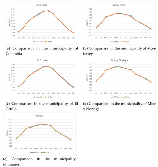
Figure 2.
Comparison between the solar irradiation calculated by the mathematical model and the one gathered from the NASA database.
Table 3.
Statistical test (model vs. NASA).
4.2. Discussion and Findings
Once the model was validated, different angles were chosen to compute the solar irradiation arriving at a solar harvesting surface, as shown in the Appendix B Table A2 and Table A3. The mathematical model was used to inquire which combinations of possible angles would allow to capture the greatest amount of solar irradiation.
Different month arrangements were formed. The azimuth value was set to zero, and the tilt angle was varied to calculate the corresponding irradiation value. Various sets and groupings of months can be selected. Table 4 shows the average results of all the combinations of all the groupings made in this paper. However, it is necessary to note the particularities of each selection.
Table 4.
Comparison of average annual solar radiation.
Table 5 proposes 12 angle changes, one for each month, that would be the most efficient in terms of capturing solar irradiation, but it is more demanding in terms of path tracking. Table 6 requires only five changes, and the average efficiency is 99.93%. If the year is divided into four periods of three months each, the efficiency remains high with an average value of 99.44% with a follow-up cost of only four angular values as shown in Table 7. Table 8 divides the year into two large groups of six months, and this selection requires only two discrete positions; however, the efficiency is reduced to 94.94%. Finally, when calculating the efficiency with a fixed angle of 25 degrees, Table 9, an efficiency of 94.35% is obtained. Although different arrangements of months can be used, as an additional example, the arrangement shown in Table 10 was formed, consisting of four partitions but considering irregular distribution of grouping the months with an efficiency of 99.94%. This is done in order to improve the efficiency of the array throughout the year. These findings have an evident impact on the design of electromechanical solar tracking systems, where the proposed mathematical model can be used as a reference of optimal angles to obtain the best possible performance.
Table 5.
The 12 months’ angle combinations.
Table 6.
Bimonthly angle combinations.
Table 7.
Quarterly angle combinations.
Table 8.
Biannual angle combinations.
Table 9.
Fixed angle combinations.
Table 10.
Alternative quarterly angle combinations.
Notice that, as discussed above, there is a difference of an almost 6% loss between leaving the tilt angle fixed and changing it every month; it is practically the same to be changing it every month as it is to be doing it quarterly.
Figure 3 illustrates the relationship between the month of the year, the tilt angle () and the solar irradiation. The aim of this figure is to provide a guide that presents how solar irradiation behaves respect to different tilt angles during the year. Additionally, Figure 3 offers an easy way to analyze data, which can be used to accelerate decision making regarding the orientation of solar harvesting systems for optimal performance or planning minimum values of solar irradiation throughout the year.
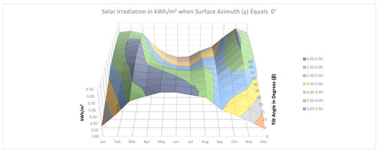
Figure 3.
Total solar irradiation throughout the year in kWh/m depending on the tilt angle when azimuth equals 0.
As can be seen in Figure 4, any relationship between the tilt angle and the received solar irradiation follows a behavior like that of a convex parabola, that is, there is a vertex where the optimum angle is found, and the further away it is from this point, in either direction, the lower the solar radiation that it receives. This effect is more visible in the first and last quarter of the year, where both branches of the parabola can be observed in all months, unlike the months of May, June and July, where the optimal angle is zero.
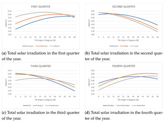
Figure 4.
Total solar irradiation throughout the year in kWh/m2, depending on the tilt angle when azimuth equals 0, broken down into quarters.
5. Conclusions
A mathematical model developed at the University of Tomsk, Russia, for high latitudes was applied to obtain a set of angles to maximize the energy collection in the state of Nuevo León, a strategic region of northern Mexico, showing excellent results, according to the evaluated metrics. The model was evaluated in specific points of the state, and was used for a particular point within the university campus of Tec de Monterrey. The viability of the model was evaluated when applied to solar harvesting surfaces to maximize energy collection. It was found that the model allows studying the angular variation of a solar harvesting surface in such a way that a set of angles was found that allows maximizing the solar energy capture. The implications of this are of interest to solar engineering, as it visualizes the possibility of designing discrete tracking systems, that is, tracking systems that vary the angles at certain discrete positions to be selected by the user throughout the year. This is a different approach to current solar tracking systems that are designed to do continuous day-to-day monitoring at a high computational and economic cost. Discrete tracking would be, according to our findings, simpler. However, more research is required in this regard.
Another implication of our findings is that this type of study can be used to improve the urban development of the region by reducing the costs of efficient solar collection systems for the generation of green energy and reducing the regional carbon footprint, due to energy production.
It is worth highlighting that, after a series of performance tests with different tilt and surface azimuth angles for a receiving surface, it was found that the azimuth angle had a minimal effect on the solar irradiation on the surface for a discrete monthly approach. On the other hand, different tilt angles represent notable variations in the solar irradiation obtained. Based on these findings, it was concluded the importance of modifying the tilt and azimuth angles in order to achieve the best efficiency of solar irradiation that can be received on a surface, such as solar panels in the analyzed location. This study presented an approach that, if the results obtained against meteorological stations are compared, the proposed method offers an effective quantitative advantage since it requires neither monitoring stations nor the operating and maintenance costs involved. These results can be utilized to assess the deployment and planning of renewable energy systems based on solar panels with adjustable angle.
Finally, as future work, applications of solar tracking and monitoring systems for photovoltaic or thermal solar implementations are proposed based on this paper; this study establishes the possibility of being used for the design of a discrete tracking system, based on Table 5, Table 6, Table 7, Table 8, Table 9 and Table 10 as inputs, which can be implemented as a sensorless open-loop control system, as conventional solar tracking systems are based on continuous angle regulation.
Author Contributions
Conceptualization, E.A.E.-V. and J.d.-J.L.-S.; methodology, E.A.E.-V., V.H.B. and L.C.F.-H.; software, G.Q.-O.; validation, G.Q.-O., E.A.E.-V. and V.H.B.; formal analysis, G.Q.-O. and E.A.E.-V.; investigation, J.C.M.-M., G.Q.-O., E.A.E.-V., V.H.B. and L.C.F.-H.; resources, J.d.-J.L.-S.; data curation, G.Q.-O. and E.A.E.-V.; writing—original draft preparation, J.C.M.-M., G.Q.-O. and V.H.B.; writing—review and editing, E.A.E.-V., V.H.B., L.C.F.-H., R.A.R.-M. and J.d.-J.L.-S.; visualization, E.A.E.-V., L.C.F.-H. and J.d.-J.L.-S.; supervision, V.H.B.; project administration, V.H.B.; funding acquisition, J.d.-J.L.-S. and R.A.R.-M. All authors have read and agreed to the published version of the manuscript.
Funding
The APC was funded by CampusCity Initiative from the School of Engineering and Sciences at the Tecnologico de Monterrey.
Institutional Review Board Statement
Not applicable.
Informed Consent Statement
Not applicable.
Conflicts of Interest
The authors declare no conflict of interest.
Abbreviations
The following abbreviations are used in this manuscript:
| EMAs | Automatic meteorological stations |
| ESIMEs | Synoptic meteorological stations |
| NASA | National Aeronautics and Space Administration |
| NASA SSE | NASA Surface Meteorology and Solar Energy |
| MAE | Mean absolute error (dimensionless) |
| MBE | Mean bias error (dimensionless) |
| MPE | Mean percentage error (%) |
| RMSE | Root mean square error (dimensionless) |
| RPE | Relative percentage error (%) |
| SMN | Mexican National Weather Service |
| PV | Photovoltaic |
| Greek Letters | |
| Tilt angle of the receiving surface with respect to the horizontal | |
| Surface azimuth angle | |
| Declination angle | |
| Latitude | |
| Longitude | |
| Surface albedo | |
| Incidence angle | |
| Solar zenith angle | |
| Solar hour angle | |
| Sunset hour angle | |
| Symbols | |
| a | Hourly transparency coefficient first variable (dimensionless) |
| b | Hourly transparency coefficient second variable (dimensionless) |
| Anisotropic index (dimensionless) | |
| Solar azimuth angle | |
| B | Equation of time coefficient (dimensionless) |
| df | T-Student degrees of freedom (dimensionless) |
| Dif GMT | Time zone hour difference with respect to Greenwich meridian (hours) |
| i | Number of the analyzed month |
| Clearness index (dimensionless) | |
| n | Number of months in the year |
| N | Day number |
| r | Correlation coefficient (dimensionless) |
| Coefficient of determination (dimensionless) | |
| Reference value for statistical analysis | |
| Calculated value for statistical analysis | |
| G | Total radiation arriving at an inclined surface (W/m2) |
| Hourly extra-atmospheric radiation arriving at a horizontal surface (W/m2) | |
| Hourly direct radiation arriving at a horizontal surface (W/m2) | |
| Hourly diffuse radiation arriving at a horizontal surface (W/m2) | |
| Hourly total radiation arriving at a horizontal surface (W/m2) | |
| Solar constant = 1367 (W/m2) | |
| h | Solar altitude angle |
| H | Average daily radiation arriving at a horizontal surface (Wh/m2) |
| Average daily extra-atmospheric insolation arriving at a horizontal surface (Wh/m2) | |
| Average daily extra-atmospheric insolation arriving at a horizontal surface (Wh/m2) | |
| Diffusion index (dimensionless) | |
| Clearness index (dimensionless) | |
| Time hr | Time of the day in hours |
Appendix A. Equations from Mathematical Model
All the equations used in the mathematical model are shown below:
Declination angle of the sun ():
The solar hour angle ():
The equation of time (EoT):
Value of B:
The incidence angle ():
The solar zenith angle ():
The solar altitude angle (h):
The solar azimuth angle ():
The sunset hour angle ():
The hourly diffuse coefficient ():
The hourly transparency coefficient ():
Values of coefficients a and b:
The clearness index ():
The average daily extra-atmospheric insolation arriving at a horizontal surface ():
Solar constant ():
The average daily radiation arriving at a horizontal surface (H):
The diffusion index ():
The average daily diffuse radiation arriving at a horizontal surface ():
can be determined by the equations and conditions shown in Table A1. is determined based on .
Table A1.
Conditional table to determine the diffusion index .
Table A1.
Conditional table to determine the diffusion index .
| Condition | Equation |
|---|---|
| if < 45 | |
| else if > 150 | |
| else if > 125 | |
| else if > 100 | |
| else if > 81.4 | |
| else |
Total ():
Diffuse ():
Direct ():
The hourly extra-atmospheric radiation arriving at a horizontal surface ():
The anisotropic index ():
Appendix B. Positive and Negative Azimuth Angle Combinations for Monterrey Tec Campus, State of Nuevo León
Table A2 presents the solar irradiation in kWh/m2 calculated using the proposed model for all combination with a positive surface azimuth angle from 0 to 15 degrees and tilt angle from 0 to 60. Table A3 shows the same but with negative surface azimuth angle from −5 to −15 degrees.
Table A2.
Positive azimuth angle combinations for Monterrey Tec campus (latitude: 25.6544 N; longitude: 100.2874 W).
Table A2.
Positive azimuth angle combinations for Monterrey Tec campus (latitude: 25.6544 N; longitude: 100.2874 W).
| Jan | Feb | Mar | Apr | May | June | July | Aug | Sept | Oct | Nov | Dec | Annual Average | ||
|---|---|---|---|---|---|---|---|---|---|---|---|---|---|---|
| 3.79 | 4.64 | 5.64 | 5.98 | 6.27 | 6.28 | 6.09 | 5.90 | 5.04 | 4.62 | 4.15 | 3.59 | 5.17 | 0 | 0 |
| 4.13 | 4.94 | 5.86 | 6.05 | 6.24 | 6.21 | 6.04 | 5.93 | 5.16 | 4.87 | 4.50 | 3.94 | 5.32 | 0 | 5 |
| 4.44 | 5.20 | 6.03 | 6.09 | 6.17 | 6.10 | 5.95 | 5.92 | 5.25 | 5.08 | 4.83 | 4.26 | 5.44 | 0 | 10 |
| 4.72 | 5.43 | 6.17 | 6.08 | 6.07 | 5.95 | 5.83 | 5.87 | 5.31 | 5.26 | 5.11 | 4.55 | 5.53 | 0 | 15 |
| 4.97 | 5.63 | 6.26 | 6.04 | 5.93 | 5.78 | 5.68 | 5.79 | 5.33 | 5.40 | 5.37 | 4.82 | 5.58 | 0 | 20 |
| 5.19 | 5.79 | 6.32 | 5.95 | 5.75 | 5.57 | 5.49 | 5.67 | 5.32 | 5.51 | 5.59 | 5.05 | 5.60 | 0 | 25 |
| 5.37 | 5.91 | 6.33 | 5.83 | 5.55 | 5.33 | 5.28 | 5.53 | 5.28 | 5.58 | 5.77 | 5.25 | 5.58 | 0 | 30 |
| 5.51 | 5.99 | 6.30 | 5.68 | 5.31 | 5.07 | 5.03 | 5.34 | 5.21 | 5.62 | 5.91 | 5.41 | 5.53 | 0 | 35 |
| 5.62 | 6.02 | 6.23 | 5.49 | 5.04 | 4.78 | 4.76 | 5.13 | 5.10 | 5.61 | 6.01 | 5.54 | 5.45 | 0 | 40 |
| 5.69 | 6.02 | 6.12 | 5.27 | 4.75 | 4.46 | 4.47 | 4.89 | 4.97 | 5.58 | 6.07 | 5.63 | 5.33 | 0 | 45 |
| 5.72 | 5.98 | 5.96 | 5.01 | 4.43 | 4.13 | 4.16 | 4.62 | 4.80 | 5.50 | 6.08 | 5.68 | 5.17 | 0 | 50 |
| 5.72 | 5.90 | 5.77 | 4.73 | 4.10 | 3.78 | 3.82 | 4.33 | 4.60 | 5.39 | 6.06 | 5.69 | 4.99 | 0 | 55 |
| 5.67 | 5.78 | 5.55 | 4.42 | 3.74 | 3.42 | 3.47 | 4.02 | 4.38 | 5.24 | 5.99 | 5.66 | 4.78 | 0 | 60 |
| 3.79 | 4.64 | 5.64 | 5.98 | 6.27 | 6.28 | 6.09 | 5.90 | 5.04 | 4.62 | 4.15 | 3.59 | 5.17 | 5 | 0 |
| 4.13 | 4.94 | 5.86 | 6.05 | 6.24 | 6.21 | 6.04 | 5.93 | 5.16 | 4.87 | 4.50 | 3.94 | 5.32 | 5 | 5 |
| 4.44 | 5.20 | 6.03 | 6.08 | 6.17 | 6.10 | 5.95 | 5.92 | 5.25 | 5.08 | 4.82 | 4.26 | 5.44 | 5 | 10 |
| 4.72 | 5.43 | 6.16 | 6.08 | 6.07 | 5.95 | 5.83 | 5.87 | 5.31 | 5.25 | 5.11 | 4.55 | 5.53 | 5 | 15 |
| 4.97 | 5.62 | 6.26 | 6.03 | 5.93 | 5.78 | 5.68 | 5.79 | 5.33 | 5.40 | 5.36 | 4.81 | 5.58 | 5 | 20 |
| 5.18 | 5.78 | 6.31 | 5.95 | 5.76 | 5.57 | 5.49 | 5.68 | 5.32 | 5.50 | 5.58 | 5.05 | 5.60 | 5 | 25 |
| 5.36 | 5.90 | 6.32 | 5.83 | 5.55 | 5.33 | 5.28 | 5.53 | 5.28 | 5.57 | 5.76 | 5.24 | 5.58 | 5 | 30 |
| 5.51 | 5.98 | 6.29 | 5.68 | 5.31 | 5.07 | 5.04 | 5.35 | 5.21 | 5.61 | 5.90 | 5.40 | 5.53 | 5 | 35 |
| 5.61 | 6.02 | 6.22 | 5.49 | 5.05 | 4.78 | 4.77 | 5.13 | 5.10 | 5.61 | 6.00 | 5.53 | 5.44 | 5 | 40 |
| 5.68 | 6.01 | 6.11 | 5.27 | 4.76 | 4.47 | 4.48 | 4.89 | 4.96 | 5.57 | 6.05 | 5.62 | 5.32 | 5 | 45 |
| 5.71 | 5.97 | 5.96 | 5.02 | 4.44 | 4.14 | 4.16 | 4.63 | 4.80 | 5.49 | 6.07 | 5.66 | 5.17 | 5 | 50 |
| 5.70 | 5.89 | 5.77 | 4.73 | 4.10 | 3.79 | 3.83 | 4.34 | 4.60 | 5.38 | 6.04 | 5.67 | 4.99 | 5 | 55 |
| 5.66 | 5.77 | 5.54 | 4.42 | 3.75 | 3.43 | 3.48 | 4.02 | 4.38 | 5.23 | 5.98 | 5.65 | 4.78 | 5 | 60 |
| 3.79 | 4.64 | 5.64 | 5.98 | 6.27 | 6.28 | 6.09 | 5.90 | 5.04 | 4.62 | 4.15 | 3.59 | 5.17 | 10 | 0 |
| 4.13 | 4.93 | 5.85 | 6.05 | 6.24 | 6.21 | 6.04 | 5.93 | 5.16 | 4.86 | 4.50 | 3.93 | 5.32 | 10 | 5 |
| 4.43 | 5.19 | 6.02 | 6.08 | 6.17 | 6.10 | 5.95 | 5.92 | 5.25 | 5.07 | 4.81 | 4.25 | 5.44 | 10 | 10 |
| 4.71 | 5.42 | 6.16 | 6.08 | 6.07 | 5.96 | 5.83 | 5.87 | 5.30 | 5.24 | 5.10 | 4.54 | 5.52 | 10 | 15 |
| 4.95 | 5.61 | 6.25 | 6.03 | 5.93 | 5.78 | 5.68 | 5.79 | 5.32 | 5.38 | 5.35 | 4.80 | 5.57 | 10 | 20 |
| 5.16 | 5.76 | 6.30 | 5.95 | 5.76 | 5.58 | 5.50 | 5.68 | 5.31 | 5.49 | 5.56 | 5.03 | 5.59 | 10 | 25 |
| 5.34 | 5.88 | 6.31 | 5.83 | 5.56 | 5.34 | 5.29 | 5.53 | 5.27 | 5.56 | 5.74 | 5.22 | 5.57 | 10 | 30 |
| 5.48 | 5.95 | 6.28 | 5.68 | 5.32 | 5.08 | 5.05 | 5.35 | 5.20 | 5.59 | 5.87 | 5.38 | 5.52 | 10 | 35 |
| 5.58 | 5.99 | 6.20 | 5.49 | 5.06 | 4.80 | 4.78 | 5.14 | 5.09 | 5.59 | 5.97 | 5.50 | 5.43 | 10 | 40 |
| 5.65 | 5.98 | 6.09 | 5.28 | 4.77 | 4.49 | 4.49 | 4.91 | 4.96 | 5.54 | 6.02 | 5.58 | 5.31 | 10 | 45 |
| 5.68 | 5.94 | 5.94 | 5.02 | 4.46 | 4.16 | 4.18 | 4.64 | 4.79 | 5.47 | 6.03 | 5.63 | 5.16 | 10 | 50 |
| 5.67 | 5.85 | 5.74 | 4.75 | 4.13 | 3.82 | 3.85 | 4.35 | 4.60 | 5.35 | 6.01 | 5.64 | 4.98 | 10 | 55 |
| 5.62 | 5.73 | 5.52 | 4.44 | 3.78 | 3.46 | 3.51 | 4.04 | 4.37 | 5.21 | 5.94 | 5.61 | 4.77 | 10 | 60 |
| 3.79 | 4.64 | 5.64 | 5.98 | 6.27 | 6.28 | 6.09 | 5.90 | 5.04 | 4.62 | 4.15 | 3.59 | 5.17 | 15 | 0 |
| 4.12 | 4.93 | 5.85 | 6.05 | 6.24 | 6.21 | 6.04 | 5.93 | 5.16 | 4.86 | 4.49 | 3.93 | 5.32 | 15 | 5 |
| 4.42 | 5.18 | 6.02 | 6.08 | 6.17 | 6.10 | 5.96 | 5.92 | 5.24 | 5.06 | 4.80 | 4.24 | 5.43 | 15 | 10 |
| 4.69 | 5.40 | 6.14 | 6.07 | 6.07 | 5.96 | 5.84 | 5.87 | 5.29 | 5.23 | 5.08 | 4.52 | 5.51 | 15 | 15 |
| 4.92 | 5.59 | 6.23 | 6.03 | 5.94 | 5.79 | 5.69 | 5.79 | 5.32 | 5.36 | 5.32 | 4.77 | 5.56 | 15 | 20 |
| 5.13 | 5.74 | 6.28 | 5.95 | 5.77 | 5.59 | 5.51 | 5.68 | 5.30 | 5.47 | 5.53 | 4.99 | 5.58 | 15 | 25 |
| 5.30 | 5.84 | 6.29 | 5.83 | 5.57 | 5.36 | 5.30 | 5.53 | 5.26 | 5.53 | 5.70 | 5.18 | 5.56 | 15 | 30 |
| 5.44 | 5.92 | 6.25 | 5.68 | 5.34 | 5.10 | 5.06 | 5.36 | 5.19 | 5.56 | 5.83 | 5.33 | 5.50 | 15 | 35 |
| 5.53 | 5.95 | 6.18 | 5.50 | 5.08 | 4.82 | 4.80 | 5.15 | 5.08 | 5.55 | 5.92 | 5.45 | 5.42 | 15 | 40 |
| 5.60 | 5.94 | 6.06 | 5.28 | 4.80 | 4.52 | 4.52 | 4.92 | 4.94 | 5.51 | 5.96 | 5.53 | 5.30 | 15 | 45 |
| 5.62 | 5.89 | 5.91 | 5.04 | 4.49 | 4.20 | 4.21 | 4.66 | 4.78 | 5.43 | 5.97 | 5.57 | 5.15 | 15 | 50 |
| 5.61 | 5.80 | 5.72 | 4.76 | 4.17 | 3.86 | 3.89 | 4.38 | 4.59 | 5.31 | 5.94 | 5.57 | 4.97 | 15 | 55 |
| 5.55 | 5.67 | 5.49 | 4.46 | 3.82 | 3.51 | 3.56 | 4.08 | 4.37 | 5.16 | 5.87 | 5.54 | 4.76 | 15 | 60 |
Table A3.
Negative azimuth angle combinations for Monterrey Tec campus (latitude: 25.6544 N; longitude: 100.2874 W).
Table A3.
Negative azimuth angle combinations for Monterrey Tec campus (latitude: 25.6544 N; longitude: 100.2874 W).
| Jan | Feb | Mar | Apr | May | June | July | Aug | Sept | Oct | Nov | Dec | Annual Average | ||
|---|---|---|---|---|---|---|---|---|---|---|---|---|---|---|
| 3.79 | 4.64 | 5.64 | 5.98 | 6.27 | 6.28 | 6.09 | 5.90 | 5.04 | 4.62 | 4.15 | 3.59 | 5.17 | −5 | 0 |
| 4.13 | 4.94 | 5.86 | 6.05 | 6.24 | 6.21 | 6.04 | 5.93 | 5.16 | 4.87 | 4.50 | 3.94 | 5.32 | −5 | 5 |
| 4.44 | 5.20 | 6.03 | 6.08 | 6.17 | 6.10 | 5.95 | 5.92 | 5.25 | 5.08 | 4.82 | 4.26 | 5.44 | −5 | 10 |
| 4.72 | 5.43 | 6.16 | 6.08 | 6.07 | 5.95 | 5.83 | 5.87 | 5.31 | 5.25 | 5.11 | 4.55 | 5.53 | −5 | 15 |
| 4.97 | 5.62 | 6.26 | 6.03 | 5.93 | 5.78 | 5.68 | 5.79 | 5.33 | 5.40 | 5.36 | 4.81 | 5.58 | −5 | 20 |
| 5.18 | 5.78 | 6.31 | 5.95 | 5.76 | 5.57 | 5.49 | 5.68 | 5.32 | 5.50 | 5.58 | 5.05 | 5.60 | −5 | 25 |
| 5.36 | 5.90 | 6.32 | 5.83 | 5.55 | 5.33 | 5.28 | 5.53 | 5.28 | 5.57 | 5.76 | 5.24 | 5.58 | −5 | 30 |
| 5.51 | 5.98 | 6.29 | 5.68 | 5.31 | 5.07 | 5.04 | 5.35 | 5.21 | 5.61 | 5.90 | 5.40 | 5.53 | −5 | 35 |
| 5.61 | 6.02 | 6.22 | 5.49 | 5.05 | 4.78 | 4.77 | 5.13 | 5.10 | 5.61 | 6.00 | 5.53 | 5.44 | −5 | 40 |
| 5.68 | 6.01 | 6.11 | 5.27 | 4.76 | 4.47 | 4.48 | 4.89 | 4.96 | 5.57 | 6.05 | 5.62 | 5.32 | −5 | 45 |
| 5.71 | 5.97 | 5.96 | 5.02 | 4.44 | 4.14 | 4.16 | 4.63 | 4.80 | 5.49 | 6.07 | 5.66 | 5.17 | −5 | 50 |
| 5.70 | 5.89 | 5.77 | 4.73 | 4.10 | 3.79 | 3.83 | 4.34 | 4.60 | 5.38 | 6.04 | 5.67 | 4.99 | −5 | 55 |
| 5.66 | 5.77 | 5.54 | 4.42 | 3.75 | 3.43 | 3.48 | 4.02 | 4.38 | 5.23 | 5.98 | 5.65 | 4.78 | −5 | 60 |
| 3.79 | 4.64 | 5.64 | 5.98 | 6.27 | 6.28 | 6.09 | 5.90 | 5.04 | 4.62 | 4.15 | 3.59 | 5.17 | −10 | 0 |
| 4.13 | 4.93 | 5.85 | 6.05 | 6.24 | 6.21 | 6.04 | 5.93 | 5.16 | 4.86 | 4.50 | 3.93 | 5.32 | −10 | 5 |
| 4.43 | 5.19 | 6.02 | 6.08 | 6.17 | 6.10 | 5.95 | 5.92 | 5.25 | 5.07 | 4.81 | 4.25 | 5.44 | −10 | 10 |
| 4.71 | 5.42 | 6.16 | 6.08 | 6.07 | 5.96 | 5.83 | 5.87 | 5.30 | 5.24 | 5.10 | 4.54 | 5.52 | −10 | 15 |
| 4.95 | 5.61 | 6.25 | 6.03 | 5.93 | 5.78 | 5.68 | 5.79 | 5.32 | 5.38 | 5.35 | 4.80 | 5.57 | −10 | 20 |
| 5.16 | 5.76 | 6.30 | 5.95 | 5.76 | 5.58 | 5.50 | 5.68 | 5.31 | 5.49 | 5.56 | 5.03 | 5.59 | −10 | 25 |
| 5.34 | 5.88 | 6.31 | 5.83 | 5.56 | 5.34 | 5.29 | 5.53 | 5.27 | 5.56 | 5.74 | 5.22 | 5.57 | −10 | 30 |
| 5.48 | 5.95 | 6.28 | 5.68 | 5.32 | 5.08 | 5.05 | 5.35 | 5.20 | 5.59 | 5.87 | 5.38 | 5.52 | −10 | 35 |
| 5.58 | 5.99 | 6.20 | 5.49 | 5.06 | 4.80 | 4.78 | 5.14 | 5.09 | 5.59 | 5.97 | 5.50 | 5.43 | −10 | 40 |
| 5.65 | 5.98 | 6.09 | 5.28 | 4.77 | 4.49 | 4.49 | 4.91 | 4.96 | 5.54 | 6.02 | 5.58 | 5.31 | −10 | 45 |
| 5.68 | 5.94 | 5.94 | 5.02 | 4.46 | 4.16 | 4.18 | 4.64 | 4.79 | 5.47 | 6.03 | 5.63 | 5.16 | −10 | 50 |
| 5.67 | 5.85 | 5.74 | 4.75 | 4.13 | 3.82 | 3.85 | 4.35 | 4.60 | 5.35 | 6.01 | 5.64 | 4.98 | −10 | 55 |
| 5.62 | 5.73 | 5.52 | 4.44 | 3.78 | 3.46 | 3.51 | 4.04 | 4.37 | 5.21 | 5.94 | 5.61 | 4.77 | −10 | 60 |
| 3.79 | 4.64 | 5.64 | 5.98 | 6.27 | 6.28 | 6.09 | 5.90 | 5.04 | 4.62 | 4.15 | 3.59 | 5.17 | −15 | 0 |
| 4.12 | 4.93 | 5.85 | 6.05 | 6.24 | 6.21 | 6.04 | 5.93 | 5.16 | 4.86 | 4.49 | 3.93 | 5.32 | −15 | 5 |
| 4.42 | 5.18 | 6.02 | 6.08 | 6.17 | 6.10 | 5.96 | 5.92 | 5.24 | 5.06 | 4.80 | 4.24 | 5.43 | −15 | 10 |
| 4.69 | 5.40 | 6.14 | 6.07 | 6.07 | 5.96 | 5.84 | 5.87 | 5.29 | 5.23 | 5.08 | 4.52 | 5.51 | −15 | 15 |
| 4.92 | 5.59 | 6.23 | 6.03 | 5.94 | 5.79 | 5.69 | 5.79 | 5.32 | 5.36 | 5.32 | 4.77 | 5.56 | −15 | 20 |
| 5.13 | 5.74 | 6.28 | 5.95 | 5.77 | 5.59 | 5.51 | 5.68 | 5.30 | 5.47 | 5.53 | 4.99 | 5.58 | −15 | 25 |
| 5.30 | 5.84 | 6.29 | 5.83 | 5.57 | 5.36 | 5.30 | 5.53 | 5.26 | 5.53 | 5.70 | 5.18 | 5.56 | −15 | 30 |
| 5.44 | 5.92 | 6.25 | 5.68 | 5.34 | 5.10 | 5.06 | 5.36 | 5.19 | 5.56 | 5.83 | 5.33 | 5.50 | −15 | 35 |
| 5.53 | 5.95 | 6.18 | 5.50 | 5.08 | 4.82 | 4.80 | 5.15 | 5.08 | 5.55 | 5.92 | 5.45 | 5.42 | −15 | 40 |
| 5.60 | 5.94 | 6.06 | 5.28 | 4.80 | 4.52 | 4.52 | 4.92 | 4.94 | 5.51 | 5.96 | 5.53 | 5.30 | −15 | 45 |
| 5.62 | 5.89 | 5.91 | 5.04 | 4.49 | 4.20 | 4.21 | 4.66 | 4.78 | 5.43 | 5.97 | 5.57 | 5.15 | −15 | 50 |
| 5.61 | 5.80 | 5.72 | 4.76 | 4.17 | 3.86 | 3.89 | 4.38 | 4.59 | 5.31 | 5.94 | 5.57 | 4.97 | −15 | 55 |
| 5.55 | 5.67 | 5.49 | 4.46 | 3.82 | 3.51 | 3.56 | 4.08 | 4.37 | 5.16 | 5.87 | 5.54 | 4.76 | −15 | 60 |
References
- Mancini, F.; Bendetto, N. Solar Energy Data Analytics: PV Deployment and Land Use. Energies 2020, 13, 417. [Google Scholar] [CrossRef]
- Kalogirou, S.A. Solar Energy Engineering: Processes and Systems, 2nd ed.; Academic Press: Waltham, MA, USA, 2014; ISBN 9780123972705. [Google Scholar]
- Sarmiento, L.; Burandt, T.; Löffler, K.; Oei, P. Analyzing Scenarios for the Integration of Renewable Energy Sources in the Mexican Energy System—An Application of the Global Energy System Model (GENeSYS-MOD). Energies 2019, 12, 3270. [Google Scholar] [CrossRef]
- Enríquez-Velásquez, E.A.; Benitez, V.H.; Obukhov, S.G.; Félix-Herrán, L.C.; Lozoya-Santos, J.d.-J. Estimation of Solar Resource Based on Meteorological and Geographical Data: Sonora State in Northwestern Territory of Mexico as Case Study. Energies 2020, 13, 6501. [Google Scholar] [CrossRef]
- Vasarevicius, D.; Pikutis, M. Solar radiation model for development and control of solar energy sources. Moksl. Liet. Ateitis 2016, 8, 289–295. [Google Scholar] [CrossRef][Green Version]
- Wijeratne, W.M.P.U.; Yang, R.J.; Too, E.; Wakefield, R. Design and development of distributed solar PV systems: Do the current tools work? Sustain. Cities Soc. 2019, 45, 553–578. [Google Scholar] [CrossRef]
- Obukhov, S.; Plontnikov, I.A.; Masolov, V.G. Mathematical model of solar radiation based on climatological data from NASA SSE. IOP Conf. Ser. Mater. Sci. Eng. 2018, 363, 012021. [Google Scholar] [CrossRef]
- Zaatri, A.; Azzizi, N. Evaluation of some mathematical models of solar radiation received by a ground collector. World J. Eng. 2016, 13, 376–380. [Google Scholar] [CrossRef]
- Belkilani, K.; Ben Othman, A.; Besbes, M. Estimation and experimental evaluation of the shortfall of photovoltaic plants in Tunisia: Case study of the use of titled surfaces. Appl. Phys. Mater. Sci. Process. 2018, 124, 1–10. [Google Scholar] [CrossRef]
- Ghenai, C.; Ahmad, F.F.; Rejeb, O.; Hamid, A.K. Sensitivity analysis of design parameters and power gain correlations of bi-facial solar PV system using response surface methodology. Sol. Energy 2021, 223, 44–53. [Google Scholar] [CrossRef]
- Ashraf, M.W.; Aaqib, S.M.; Manzoor, H.U.; Asharaf, M.W.; Manzor, T.; Sethi, M.H. Optimization of PV Modules through Tilt Angle in Different Cities Of Punjab, Pakistan. In Proceedings of the 2020 IEEE 23rd International Multitopic Conference (INMIC), Bahawalpur, Pakistan, 5–7 November 2020; pp. 1–5. [Google Scholar] [CrossRef]
- Estaciones Meteorológicas Automáticas (EMAS). Available online: https://smn.conagua.gob.mx/es/observando-el-tiempo/estaciones-meteorologicas-automaticas-ema-s (accessed on 7 July 2021).
- Valdes-Barrón, M.; Riveros-Rosas, D.; Arancibia-Bulnes, C.A.; Bonifaz, R. The Solar Resource Assessment in Mexico: State of the Art. Energy Procedia 2014, 57, 1299–1308. [Google Scholar] [CrossRef]
- National Aeronautics and Space Administration. NASA POWER—Prediction of Worldwide Energy Resources. Available online: https://power.larc.nasa.gov/ (accessed on 8 July 2021).
- Google. Google Earth. Available online: https://earth.google.com/web/ (accessed on 7 July 2021).
- Benítez Baltazar, V.H.; Torres Valverde, G.A.; Gámez Valdéz, L.A.; Pacheco Ramírez, J.H. Sistema fotovoltaico de iluminación solar. Epistemus 2013, 15, 86–92. [Google Scholar]
- Despotovic, M.; Nedic, V.; Despotovic, D.; Cvetanovic, S. Review and statistical analysis of different global solar radiation sunshine models. Renew. Sustain. Energy Rev. 2015, 52, 1869–1880. [Google Scholar] [CrossRef]
- Soulouknga, M.H.; Falama, R.Z.; Ajayi, O.O.; Doka, S.Y.; Kofane, T.C. Determination of a Suitable Solar Radiation Model for the Sites of Chad. Energy Power Eng. 2017, 9, 703–722. [Google Scholar] [CrossRef]
- Besharat, F.; Dehghan, A.A.; Faghih, A.R. Empirical models for estimating global solar radiation: A review and case study. Renew. Sustain. Energy Rev. 2013, 21, 798–821. [Google Scholar] [CrossRef]
- ITESM. DistritoTec es el Lugar Donde se Viven las Grandes Ideas. Available online: https://distritotec.itesm.mx/acerca/ (accessed on 5 July 2021).
- Tamhane, A.C. Statistical Analysis of Designed Experiments: Theory and Applications; John Wiley & Sons, Inc.: Hoboken, NJ, USA, 2009; pp. 627–643. [Google Scholar] [CrossRef]
Publisher’s Note: MDPI stays neutral with regard to jurisdictional claims in published maps and institutional affiliations. |
© 2021 by the authors. Licensee MDPI, Basel, Switzerland. This article is an open access article distributed under the terms and conditions of the Creative Commons Attribution (CC BY) license (https://creativecommons.org/licenses/by/4.0/).