Article

Modelling Bidding Behaviour on German Photovoltaic Auctions

Regional Centre for Energy Policy Research, REKK, Corvinus University of Budapest, 1093 Budapest, Hungary
Energies 2021, 14(2), 516; https://doi.org/10.3390/en14020516
Submission received: 13 November 2020 / Revised: 8 January 2021 / Accepted: 12 January 2021 / Published: 19 January 2021

Abstract

:
In this article renewable energy support allocation through different types of auctions are assessed. The applied methodological framework is auction theory, based on the rules governing the German photovoltaic (PV) Feed-in Premium (FIP) auctions. The work focuses on bidding strategies based on an extended levelised cost of electricity (LCOE) methodology, comparing two different set of rules: uniform price and pay-as-bid. When calculating the optimal bids an iteration is developed to find the Nash-equilibrium optimal bidding strategy. When searching for the bid function, not only strictly monotone functions, but also monotone functions are considered, extending the framework typically applied in auction theory modelling. The results suggest that the PV support allocation in the German auction system would be more cost efficient using the uniform pricing rule, since many participants bid above their true valuation in the pay-as-bid auction Nash-equilibrium. Thus from a cost minimising perspective, the application of uniform pricing rule would be a better policy decision.

1. Introduction

The topic of this article is the allocation of renewable energy support through auctions. The applied methodological framework is auction theory, based on the rules governing the German photovoltaic (PV) Feed-in Premium (fip) auctions. The work focuses on participants’ bidding strategies. The main research question is how cost reduction of RES projects and pricing rules of the auction affect the bidding and through that the support budget. Can one pricing rule bring better results—lower overall budget—than the other in an environment where many participants do not even need any support?
The costs of the bidders are calculated based on an extended lcoe (levelised cost of electricity) methodology. Income is included during and after the support period, since the project lifetime usually exceeds the support period. This uses an own electricity wholesale price forecast and a distribution for investment costs, that generates an empirical distribution for the modified LCOE values (indicated as lcoe’). This lcoe’ fits into the auction theoretic framework, serving as the valuation of the participants, which is the minimum strike price each bidder is willing to accept in order to realise its renewable energy generation project.
To answer the research question two different systems are analysed in this work. The first is the uniform price auction, where—as it is already proved in the literature, see, e.g., [1]—all participants bid their true valuation. The second is pay-as-bid, which allows strategic bidding, and is far more complex to model.
Compared to a “traditional” auction, the bidding is reversed. Typically the announcer of the tender is the so-called seller, but in this case the announcer is a buyer, and all the participants (the bidders) are sellers. This way the bid represents the support level, that is acceptable for the bidders to realise their renewable projects. Thus, the winners would be the ones with the lowest bids.
The optimal bids are calculated throughout the work using an iteration that leads to the Nash-equilibrium optimal bidding strategy. When searching for the bid function not only strictly monotone functions are considered, but monotone functions as well, that extands the framework typically applied in auction theoretic modelling. For a monotone, but not strictly monotone bid function in a multiobjective auction, the revenue equivalence theorem may not be met—as demonstrated by the results of this analysis.
While the model is rather specific (referring to the German PV auction rules) the technique (the iteration for optimal bid functions) itself is more applicable and is an important contribution to the literature. This may help find Nash-equilibriums, when the expected revenues differ between the two pricing rules.
The auction is simulated using the optimal bidding strategy for the players, and results for each pricing system are compared (e.g., highest and lowest winning bid, total support expenditure, etc.) to each other and the latest available results of the real German PV auctions.
The finding that total costs (total support allocated for the given capacity) are higher for the pay-as-bid pricing rule than for the uniform pricing is an important policy conclusion for decision makers still in the process of fine-tuning renewable auction frameworks. Though several other factors need to be considered, hopefully this work can also contribute to the discussion.

Motivation and Relevance

With the need for massive renewable energy capacity growth to achieve the energy transition, choosing the right renewable energy support scheme is all the more important. This connection between climate and energy policy is also reflected in the European policy framework, with former National Renewable Energy Action Plans (nreaps) replaced by integrated climate and renewable energy related document, the National Energy and Climate Plan (necp). The submission of the first draft version was due at the end of 2018, and the final documents a year later.
For all European Union (EU) member states renewable energy utilisation needs to be increased: to facilitate this process, the EU sets different renewable energy share targets. Targets for 2020 [2] and 2030 [3] were set differently. In case of the first, national targets were introduced, while the 2030 targets are to be achieve by the EU as a whole. There was also a common target for the EU for 2020, but then this was translated to national targets, taking into account the different position and thus possibilities of different countries (both from an economically and a renewable potential point of view). The following three targets were set for 2020:
  • 20% cut in greenhouse gas emissions (from 1990 levels);
  • 20% of EU energy from renewables;
  • 20% improvement in energy efficiency.
The 2030 targets were set with an entirely different logic. The first step was also to specify the EU level targets, which are the following:
  • At least 40% cuts in greenhouse gas emissions (from 1990 levels);
  • At least 32% share for renewable energy;
  • At least 32.5% improvement in energy efficiency.
These targets—unlike the 2020 ones—remained to be set for the EU as a whole. This brings us to the question of “gap filling”—what will happen if approaching 2030 it seems the EU can not reach the target, how can countries be forced to do more? It is possible that a central approach would be taken, some kind of a central, European support scheme can be introduced. One idea is to organise a central auction, financed by Member States (or those Member States that seem to lag behind), while renewable projects can come from any member state [4].
Latest renewable energy share statistics [5] are only available for 2019, not for 2020 yet (see Figure 1). Partly as a result of the coronavirus crisis, that led to lower consumption levels, partly because of increasing renewable capacities for 2020 numbers were most probably even higher, but it is not easy to tell yet whether the EU as a whole was able to reach the target or not, and it is even a greater challange to estimate this on a country level. Green recovery, however, was one of the buzzwords in 2020, and by the end of the year European Union leaders have agreed on an even higher target for 2030: the goal is to cut greenhouse gas emissions by at least 55% by compared with 1990 levels. All this underlines the importance of renewable energy related investments, especially in the flagship electricity sector.
European Union legislation regulates the way renewable support can be allocated in the electricity sector [6]. Early support schemes more than a decade ago led to over subsidising of renewables in several countries, including Spain, Slovakia or the Czech Republic. Cost reductions in renewable technologies were moving faster than the regulators could respond to with commensurate support levels. This was the driver behind the introduction of a new, competition based support allocation mechanism: auctions.
As a result of the new legislation (and also learning from others’ mistakes) several countries have already implemented renewable support auctions in recent years across Europe (e.g., Denmark, France, Germany, The Netherlands, Italy, Ireland, the United Kingdom, Portugal [7] and also Hungary in 2019 and in 2020 as well), and beyond, in other parts of the world: Zambia [8], Peru [9], Brasil and South Africa [7]. Energy Community Contracting Parties—Albania, Montenegro, North Macedonia—have already organised renewable support auctions [10]. These developments make this research relevant and timely, as decision makers across Europe are in the process of fine-tuning the rules of their auctions.
Germany is the logical candidate to serve as a basis for the modelling, as one of the pioneers in renewable energy utilisation and support, the so-called Energiewende started back in the 1990s. Germany has made significant strides, more than tripling renewable electricity generation capacity in 2002 from 18.5 GW to around 74 GW by 2019 [11].
Germany started renewable auctions in 2014, and now organises at least three auctions every year. With experience from pilot tenders and auctions themselves the rules were fine-tuned year after year. This makes the German system ideal to analyse and model. The key rules of the German PV auctions are the following:
  • Technology specific tenders, only PV projects can apply (there are special combined wind and PV auctions also, but they are out of the scope of this work).
  • The support is a one-sided floating premium (participants bid price level (a strike price), if market prices are lower, they are compensated and if higher they can keep the total income).
  • Support period is 20 years.
  • Project size is between 0.75 for ground-mounted PV (MW) and 10 MW.
  • A bid bond of 50 €/kW needs to be provided by participants.
  • A single sealed pay-as bid auction is organised (some of the former auctions applied uniform pricing rule)
  • A price cap is set for the strike price, adjusted according to a pre-set methodology.
  • Every year at least 3 auctions are organised (usually in February, June and October), for close to 200 MW, which can be modified according to the installed capacities in the country.
  • Project promoters have a 2 year period to realise the investment to remain eligible for the support with the original conditions.
  • Support retracted for periods with at least six consecutive hours of negative prices (based on EU rules).
Most of the above rules are incorporated into the model, but some are left out to keep the model simple enough to make precise assessment of bidding behaviour.
To sum up, renewable auctions are very important tools to achieve the EU targets in a least-cost way. It is important to understand the behaviour of participants, and plan auctions that incentive players to bid according to true costs, so that countries do not provide excessive subsidies.

2. Applied Methodology

In this section, first I highlight the most important former research connected to my work. Then I summarise the most important assumptions underpinning the modelling framework.
This begins with an overview of the calculation of bidders’ costs (valuation), that improve the existing lcoe calculation methodology using an electricity wholesale price forecast as an input for the lcoe’ calculation.
Then the auction model is presented in detail, with the necessary changes to arrive at the German PV auctions. Finally, the iteration searching for the Nash-equilibrium bid function is explained conceptually.

2.1. Former Research

Auction theory is a more and more popular research field. Its importance is also underlined by the latest Nobel-prize winners from 2020: Milgrom and Wilson “for improvements to auction theory and inventions of new auction formats”.
Since the start of auction, in theoretical research it is very typical to compare different pricing rules [12,13], both for single unit and multi-unit auctions. First price and second price auctions (or for multi-unit auctions: uniform pricing and pay-as-bid pricing) are the two mostly compared cases.
While some took a more theoretical approach (e.g., [14,15,16]), others observed electricity markets ([17,18,19,20]), or different online marketplaces (e.g., [21,22]).
Many researchers try to find how close the bids are to the true valuation of the participants, to determine how high the incentive is for “telling the truth”. According to the theoretical results [23] bidding according to the true valuatio is a (weakly) dominant strategy under uniform pricing, with some constraints. This makes the uniform price auctions a good basis of comparison to find out what is the “cost of letting participants lie”. In a pay-as-bid auction the question is how different are the bids?
As alluded to above, renewable support auctions are relatively young, outside of the UK in 1990, Ireland in 1995 and France in 1996 [24] coming after 2000. It follows that the literature itself is also in its early phase.
Besides effectiveness of auctions compared to administratively set support levels [25,26,27] many different aspects of auction rules can be analysed, including the role of penalties, state ownership, or reserve prices [28]. It is also typical to go beyong theoretical models, with experiments and simulations feeding analyis of empirical results [29,30,31], comparing different rules (pricing and technology specific or technology neutral auctions).
The starting point of this model is the theoretical premise of [32,33] for German renewable auctions, assuming fixed number of players, across each category. In their model for uniform pricing all participants bid their true costs, while for pay-as-bid participant bid after an optimisation process. At this point an assumed common knowledge distribution is applied to other bids (assuming normal distribution). The authors analyse several consecutive auctions, and apply learning. This paper only applies modelling to one auction, and applying the iteration to find the Nash-equilibrium bid functions. The starting point of the iteration, however, uses a similar bid distribution assumption.
In reality participants likely do not bid according to a Nash-equilibrium bidding strategy, which would require very sophisticated calculations. However, finding Nash-equilibrium is an interesting research proposal in any auction theory (or game theory) model. Besides the L C O E calculation and values, this will add to the literature a comparison of the outcomes for the two pricing rules.

2.2. Modified Lcoe Calculation

The Levelised Cost of Electricity (LCOE) value stands for the cost per unit of produced electricity taking into account all costs during the lifetime of the investment. This can be translated to the income per produced electricity unit that makes the net present value of incomes equal to the net present value of costs—thus it answers the question: what is the minimum fix income need (in €/MWh) that makes the investment profitable.
The common approach in the literature for calculating LCOE values to compare different technologies leaves relatively large amount of data for the estimation of the LCOE value of German PV investments. The German Energiewende is well-known and popular research topic, and because many projects have already been realised inrelation, actual cost data is also available.
As this approach is widely used, only detailed calculation of the modified lcoe are included here. The inputs used in the calculation of this paper and in the literature are summarised in Table 1. The assumptions for the former are placed in the last column, including real values for all cash-flow elements, expressed in E U R 2019 . Own estimation is applied to year 2020 (the research was carried out between March 2018 and August 2020, with some minor final modifications in the revision phase from December 2020 to January 2021).
Another important input for the calculation is the amount of total electricity generation from the PV plant, assuming the same generation profile that is used in the model applied for electricity price forecast. This is the European Electricity Market Model (EEMM), developed by REKK (Regional Centre for Energy Policy Research), (for details, see [39]). In the model all generation curves are based on historical data from the entso-e Transparency Platform ([40]). These data are adjusted so that only 24 types of hours are differentiated—within the day and within the year. This is a simplification, however, hours of the year can be put into 24 relatively homogenous groups from a PV generation point of view.
The assumed profile is presented on Figure 2.
Considering all above, the results of the own lcoe calculation are presented on Figure 3.
Significant differences between the sources can be observed, and also in some cases the same institute/research provides a wide range of data. The result of this own calculation based on the above presented inputs is 70 €/MWh. Changing the wacc (weighted average cost of capital) value to 7% ceteris paribus brings this to 88 €/MWh, while a (ceteris paribus) lower investment cost (600,000 €/MW) results in only 56 €/MWh. Calculating with a 20 years pay-back time instead of 25, the LCOE is 78 €/MWh. These are in line with the numbers from the literature, international estimations being somewhat higher, and German Fraunhofer somewhat lower.
In this auction theory model the LCOE value is calculated according to the above presented logic and can not be treated as the cost of participants (or using the auction theory terminology as their valuation). This is becuase the support is not the total income per unit of generated electricity, but the premium that is paid if the electricity wholesale prices are not “high enough”. The other factor is, 25 years lifetime compared to the 20 years support period.
As a first step, the difference between lifetime and support period must be accounted for. In the first 20 years the income can come from the market, and the state (in a form of a premium), and it can come only from the market in the last 5 years.
The Feed-in Premium (FiP) support system—or the so-called one-sided sliding premium used in Germany—begins with an investor needing to sell electricity on the market. If the received price is lower than the strike price from the auction then the investor will receive a premium, that amounts for the difference. If the market price is higher, the investor keeps the total amount and the state does not have to pay anything. This is very similar to the older Feed-in Tariff (FiT) support scheme, under which the investors had little price related risks, with the state purchasing all of the generated electricity at a pre-fixed price (“Tariff”).
Still, there remains some risk in the FiP system, as the support (the premium) is not calculated for every hour, but only at the end of each month. The first step is the calculation of the monthly reference price, that is the actual, PV generation weighted average wholesale (day-ahead) electricity price. The support is the difference between the strike price and this reference price. Each producer receives a support (in €/MWh) for each unit of electricity generated.
This means that if the average wholesale price weighted with the producer’s own generation is higher than the reference price, the total support will be higher, compared to the hourly settlement situation. If the generator’s own average wholesale price is lower than the reference price, then the monthly settlement support will be lower compared to the hourly settlement. This can incentivise producers to adjust their generation profile—if it is possible [41], but it is not something used in this model where the generation curves are assumed to be the same for all producers. This way the total support to be paid only differs by a few percentage points for monthly and hourly settlements.
The second part of the modification is the inclusion of additional incomes. Additional incomes arise when the strike price is lower than the (reference) market price. In some periods the total income per MWh will be even higher than the strike price.
Taking all this into account, the modified LCOE (from now on indicated as L C O E ) will show the minimum strike price for a profitable investment (assuming the mentioned wacc values), using the following calculation:
L C O E t = 1 N m = 1 12 E t m ( 1 + r ) t + t = 1 N m = 1 12 [ p t m L C O E ] + E t m ( 1 + r ) t + t = N + 1 n m = 1 12 p t m E t m ( 1 + r ) t = I + t = 1 n M t ( 1 + r ) t
where n = 25 years, N = 20 years, p t m is the reference electricity price of month m in year t, E t m is the total amount of generated electricity in month m of year t, L C O E is the strike price that makes the NPV of total income equal to the NPV of total cost, (assuming r discount rate, that equals to the assumed wacc value).
If the income from the market is not sufficient to turn the project positive, then it can be proven that there is exactly one L C O E value, that makes the NPV of incomes and costs equal (because the parts of the function containing L C O E are strictly increasing).
This way, the modified L C O E can be calculated, but still, it does not fit into the auction theory methodology. To have a distribution of the L C O E values not a given or fixed value is assumed for the investment cost but a distribution. It would be possible to assume that generation and wholesale prices are stochastic, but this would make the model too complicated, so both generation profiles and wholesale prices are fixed, and common knowledge to all participants.
With investment costs, participants only know the distribution, except for their own investment cost, that they know precisely. Based on this distribution, the distribution of the L C O E value can be calculated, providing a distribution of the valuation of the players.
The distribution of the investment costs is specified according to the literature. The central limit theorem states, that if a random variable can be formed as a sum of many independent random variables, then its distribution is normal. We can think of the investment cost as the sum of the price of the PV panel, the price of the site, the installation costs, the transportation costs, etc. Thus, normal distribution is assumed for the investment cost.
Two parameters still need to be defined: expected value and variance. For the former the above presented estimation 800 €/kW is applied. For variance a well-known property of every normal distribution is used. This is the so-called 3- σ -rule. It states that the probability of a realisation being no further from the expected value than “one standard deviation” ( σ ) is 68.3%. This means, that the probability that the absolute value of the difference between a random realisation and the expected value is smaller than σ is 68.3%.
P ( μ σ < x < μ + σ ) = 0.683
The same probabilities for two and three standard deviations are 95% and 99.7%. So when a random realisation is generated with a probability of 95% and 99.7% it will be no smaller than the expected value minus 2 and 3 σ , and no larger than the expected value plus 2 and 3 σ , respectively.
P ( μ 2 σ < x < μ + 2 σ ) = 0.9545
P ( μ 3 σ < x < μ + 3 σ ) = 0.9973
Using this rule, the distance of the different estimations from the expected value (800 €/kW) can be calculated, thinking of them as realisations of the sought distribution. Since the numbers from Lazard (2017), and the upper values for 2018 (IRENA) seem to be outliers, they are not taken into account—they are assumed to be realisations with very small probability. The calculated distances (absolute values of the difference of the realisation and the expected value) are the following Table 2.
Based on these calculations the values from the literature seems to be in a range of ( 200 ; + 155 ) €/kW distance from the expected value (800 €/kW). If this distance is assumed to be 2 σ long, then the appearance of the outliers is an event with a 1 − 0.9645 = 3.5% probability. Based on that, the assumed distribution for the investment cost is: I N ( 800 , 100 ) (where 100 is the standard deviation).
The last step to calculate the distribution of the L C O E is a forecast of electricity prices over the next 25 years, using the eemm model.
The eemm covers 41 markets in 38 European countries. For every country a separate demand curve is assumed, and on the supply side all power generation units are included on a block level except renewable generators, where only the total installed capacity is used. Each model run simulates one hour with no connection between the different simulated hours. The equilibrium wholesale prices are calculated from the demand-supply balance, taking into account domestic generation units and the possibility of cross-border trade.
The model assumes perfect competition: generators offer electricity on a marginal cost basis (merit-order curves are calculated for each market), market participants are price takers and there is no capacity withholding, by producers or operators of interconnectors. The model maximises the producer and consumer welfare throughout the whole modelled region. For further details on the modelling (including inputs and assumptions), see: [42,43] (Most of the inputs are the same as the ones used for the seermap—South East European Roadmap modelling, a cooperation between rekk and Energy Economics Group of TU Wien).
Future electricity prices have an important role in this calculation, both in the support period (possible additional income above the support), and in the last five years of the lifetime, where only incomes from the wholesale market are assumed. There is of course some uncertainty in this price forecast, as in every modelling, but having hourly differentiated prices can still be considered a rather sophisticated approach (e.g., in contrast to calculating with yearly average prices).
Results of the calculation are presented in the following section.

2.3. The Modelling Framework

This model is based on the general auction theoretic framework, where participants are rational and risk neutral. The given distribution for their valuation is common knowledge among everyone. The auction is symmetric with the same valuation distribution for all. Participants know their own valuation realisation, but do not know the exact valuation of others (only its distribution). The players optimise their bid to have the highest expected utility.
While participation is not free in the German PV auctions (e.g., because of the bid bond, and other administrative burdens) it is a normal approach in the literature so that the utility of losing is 0. Thus, the formula of expected utility is reduced to the probability of winning multiplied by the utility of winning.
The literature typically also assumes strictly monotone bid functions, whereby the probability of winning can be calculated from the valuation distribution of others. In case of monotone (but not strictly monotone) bid functions, however, this is not the case. In this situation, the probability of winning can be calculated from the distribution of others’ bids, which can differ from the distribution of their valuations.
In order to be able to calculate the bid distribution we need to know or assume something about the optimal bid function. The literature has two methods for this: (i) finding the Nash-equilibrium bidding strategy, revealing the bid functions that are best responses to the bid functions of other players (see details in Section 2.1) (the bid function that is the best response is the one, that gives the utility maximising bid in case of all valuations when the bid functions of other players are fixed); and (ii) making some simplifications. Instead of finding the Nash-equilibrium, participants make assumptions regarding the behaviour of other participants, and optimise their bids accordingly (e.g., [32,33]).
The model used in this study combines these two approaches: the iteration with a starting assumption regarding the bid distributions, then searching for the Nash-equilibrium bid functions.

The Model of the German PV Auction

This section provides a deeper introduction to the German PV auction system applied to the modelling for this study. Some of the original rules are left out for simplicity to focus on the bidding behaviour of participants.
The German PV auction applies a pay-as-bid rule, where the constraint is given in capacity (MWs). The sliding (or floating) premium is measured as €ct/kWh but for the purpose of this study €/MWh is used (as wholesale electricity prices are also typically published in €/MWh). The support is specified for every generated unit (MWh) of electricity.
The capacity constraint was close to 200 MW across all auctions in 2017, 2018 and 2019, the exact amount is provided in Table 3. So this is used as the capacity constraint for this model. Table 4 and Table 5 show the number of participants of former auctions and average project size.
Taking into account all of these data this modelling exercise assumes 100 auction participant, with a project size of 5 MW, entirely symmetric participants, meaning that all simulated auctions will result in exactly 40 winners and 60 losers.
There are two reasons for assuming symmetry: first, this is a technology specific auction, so projects should be similar, and second, there is no information on the possible differences (e.g., type of participants or location of projects).
After defining all inputs and assumptions the expected profit function can be formalized. As presented above, this consists of the probability of winning multiplied by the utility of winning. Hereinafter expected profit means the expected profit for each generated unit of electricity. This way the same measurement unit applies for the valuation, the bid, the strike price and the expected profit. With fixed generation profile and future electricity prices the model stays general, as for every expected profit (in €/MWh) the total expected profit can be calculated throughout the lifetime of the project (in €).
Thus, the expected profit, that equals the expected utility can be formalized by the following:
U j , w = b j L C O E j ,
where:
  • U j , w is the utility of winning for participant j
  • ( b j ) is the bid of participant j;
  • L C O E j is the valuation of participant j.
In order to calculate the probability of winning a bid distribution of others must be assumed. As mentioned above, for only strictly monotone bid functions the valuation distribution would be enough, but for monotone but not strictly monotone bid functions the bid distribution is needed. Let the assumed bid distribution function be F.
The logic of the model is the following. Participant j can win, if there is only maximum 39 other participants with a bid lower than his. The probability of any participant’s bid being lower (or equal) than the bid of participant j ( b j ) is F ( b j ) (as this is the definition of function F). The probability of any participant’s bid being higher than b j is 1 F ( b j )
Participants also calculate the possibility of a tie. In a scenario of equal bids, the number of total winners does not change, and some of the bidders will be chosen randomly.
All in all, the following probability needs to be calculated: a maximum 39 bids being lower than b j , and either no other bidder with the same bid ( b j ), or if bidder j is part of a tie with the rest, he will be chosen randomly as a winner. Thus, from the probability of “there is maximum 39 bids being lower than b j ” the probability of “in that case there is a tie, and bidder j is not chosen randomly as a winner” is deducted.
When this probability is calculated we need to take into account, that any 39, 38, 37, etc. participant can put forth lower bids leading to different outcomes. These participants can be chosen in 100 39 , 100 38 or 100 37 different ways. A similar logic applies to the tie situation.
Now all variables known to formalize the probability of winning. Following the previous notation for participant j the probability of winning with bid b j is the following:
P j , w ( b j ) = i = 0 39 100 i F ( b j ) i ( 1 F ( b j ) ) 100 i ( 1 i = 0 39 l = 1 100 i 100 i l P ( b j ) l ( 1 P ( b j ) ) 100 i l ( 1 min ( 40 i ; l + 1 ) l + 1 ) )
This leads to the expected profit (or utility) function:
E ( π j ( x j , b j ) ) = P j , w ( b j ) U j , w = i = 0 39 100 i F ( b j ) i ( 1 F ( b j ) ) 100 i ( 1 i = 0 39 l = 1 100 i 100 i l P ( b j ) l ( 1 P ( b j ) ) 100 i l ( 1 min ( 40 i ; l + 1 ) l + 1 ) ) ( b j L C O E j )
This is the function that needs to be maximised in b j for a given L C O E . The distribution of the bids can be found using a simulation: for 10,000 different L C O E values (valuations) the optimal bid ( b j ) can be calculated, meaning 10,000 different bid realisations will lead to the distribution. The bid function can also be found by connecting the valuations and the bids.

2.4. Finding Nash-Equilibrium

This section explains in detail the applied methodology for searching for a Nash-equilibrium bidding strategy for uniform pricing and pay-as-bid pricing rules. As they are significantly different, they are analysed separately.

2.4.1. Uniform Price Auction

As mentioned before, a uniform pricing rule dose not reuqire an optimisation algorithm. A simple deduction can lead to the solution without any assumption for other players’ bids (similar reasoning is included in (Krishna, 2010). This is because support received by the winners are not in direct connection with their own bids. Winners are the ones with the lowest bids, but the support they win is the lowest non-winning bid—which is higher per definition than their bids. This way none of the winners are price setters, they all receive a higher support than their own bid.
To maximise their expected utility they have to increase the probability of winning, and the utility of winning. Under pay-as-bid auctions these two values can not be increased at the same time (see details below). In a uniform pricing auction, however, the utility of winning does not depend on the participant’s own bid, only the lowest non-winning bid, which the participants have no influence over (through their own bids).
Thus, the probability of winning can be increased without decreasing the utility of winning up until the point that the bid is not lower than the L C O E . When it goes below the valuation, the price setter’s bid can be lower than the valuation of the winner, making the utility of winning negative. To avoid this, the lowest bid should be the L C O E , which is also the optimal bid, because the lowest bid maximises the probability of winning.
This way the optimal bidding strategy is to “tell the truth”, bidding according to the valuation. As this strategy is the optimal one regardless of other players’ bids, it is always the best response to others’ bids, so the identity function as the bid function will lead to a Nash-equilibrium.

2.4.2. Pay-as-Bid Auction

Finding the pay-as-bid auction Nash-equilibrium bidding strategy is more complex, requiring the creation of a searching algorithm.
When maximising the expected utility the bid itself influences not only the probability of winning but also the utility of winning, with the participant’s bid serving as its own strike price. Bidding higher will increase the latter, but decrease the former—so a more sophisticated algorithm is needed to find the optimal bid. In this situation the bidding strategy does depend on the bidding strategy of others, so the assumptions become very important.
In the literature, there are several ways for searching for or even calculating (if possible) Nash-equilibrium bidding strategies. One group of algorithms are connected to solving differential equations. In case of bid functions that have an inverse a typical approach is to write the formula that leads to a differential equations, of which the solution is the equilibrium bid function. However, many times these equations can not be solved without a numerical iteration algorithm. This approach is followed by, e.g., [45,46,47]. As this work covers non-strictly monotone bid functions as well, this approach is not followed here.
Ref. [48] searches for Bayes Nash Equilibrium (bne) assuming discrete bids and valuations on a single object auction. Authors analyse situations with different valuation distributions and number of players and compare pay-as-bid and uniform pricing. In each iteration they calculate the best response assuming a price distribution. From these a new price distribution can be calculated, and is set as the assumed distribution for the next iteration step. They stop once the assumed and the resulting distributions are identical. In case of uniform pricing, they arrive to the equilibrium in only 2 steps, and they got back the well-known result: bidding true valuation is the optimal strategy. In case of pay-as-bid auction the number of iteration needed depends on the starting assumptions, but on average 5 steps are needed.
Similar logic is used by [49], who analyses simultaneous ascending auction, that allocates a set of M related goods among N agents via separate auctions for each good. They define the so-called self-confirming predictions the following way: a prediction is self-confirming if, when all agents follow the same predictor bidding strategy, the final price distributions that actually result are consistent with the utilized characteristics of the prediction.
This idea is also very close to the equilibrium definition used by [50]: we are in a fulfilled expectations equilibrium, if when each firm uses its model and maximizes expected profit, the joint distribution of signals and residual demand functions that is realized is precisely the one given by its model. So once again, the main idea is to have a consistency between assumed and resulting behaviour. That is what the following iteration also tries to capture.
  • As a first step, a given bid distribution is assumed for other participants, and the optimal bidding strategy (the best response) is calculated.
  • The next step compares the distribution of bids (taking into account the distribution of valuations) coming from the best response of every player to the assumed bid distribution. If they are equal, Nash-equilibrium has been reached. If not, this new bid distribution will be assumed in the next step for other players’ bids.
  • With this new bid distribution assumption, the optimal bids (for every possible valuation) can be calculated again, and checked for Nash-equilibrium.
  • The iteration stops, when the best response is the same bidding strategy as the one assumed for other players. In this case (because of symmetry) every players’ bidding strategy is the best response for other players’ bidding strategy.
The starting point of the iteration is a normal distribution for others’ bids. The parameters of the assumed normal distribution in this model are dfined as the parameters of the empirical L C O E distribution: the expected value is 65.84, while the variance is 4.49. This normal distribution is F 1 .
Based on [51,52] the stopping criterion in this algorithm is to have a lower than 0.2% NRMSE value when comparing the resulting bids in case of step i and i-1. When the iteration arrives to that point Nash-equilibrium is found.

3. Results and Discussion

3.1. Modified Lcoe Calculation

After all the above inputs are in place the L C O E values can be calculated. First, the L C O E is calculated using an 800 €/kW investment cost, arriving to 70.38 €/MWh.
It is worth noting that for the “simple” LCOE value, the support period was set equal to the lifetime of the project, so this value should be lower than the 20-year lifetime simple LCOE while somewhat higher, than the 25-year lifetime (and support period!) simple LCOE. The difference, however, is rather small, because in the last 5 years the wholesale market prices are close to the L C O E outcome, and in the first 20 years there is some—but not much—additional income from the higher than L C O E wholesale prices.
The value of this small additional income can be quantified assuming a FiT system (or a two-sided FiP) for 20 years—the period which producers receive a fixed price, and then 5 additional years on the wholesale market. The L C O E under these assumptions is 70.42 €/MWh. This means, that the “value” of the possibility to keep the difference between market prices and the strike price (if the first one is higher) accounts for 70.42 − 70.38 = 0.04 €/MWh.
Another very important quality of this modified calculation is that the income side includes several items, not only the income from the support. This way it is possible for the project to turn profitable without any support. If the investment cost is low enough and the electricity price high enough, the L C O E value can be 0.
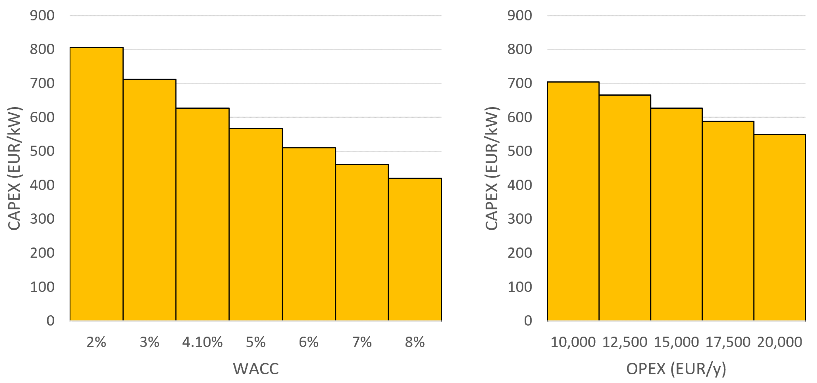
This way, the “critical investment cost” (if all other inputs are fixed) can be calculated: which is the investment cost level to make the project profitable without any support. Put another way, this is the investment cost that makes the NPV of incomes and costs equal without any support. For a critical investment cost, the L C O E will be exactly 0. This value can be calculated with different inputs: as shown on Figure 4, changing wacc (weighted average cost of capital) values and different opex (operation and maintenance) costs result in different critical investment costs.
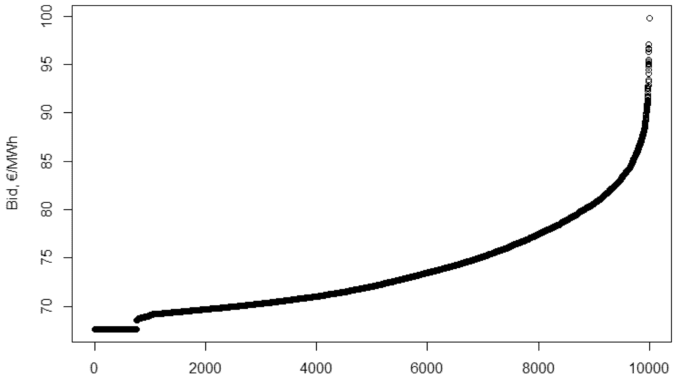
After calculating the L C O E value with different fixed investment costs the distribution of L C O E has to be calculated, based on the assumed distribution of the investment cost. As stated above, the L C O E calculation is an optimisation: 10,000 investment cost values are simulated using the assumed distribution to calculate the L C O E values. This provides an empirical distribution of the L C O E value. For investment costs lower than the “critical investment cost”, 0 support is needed this is the minimum, since no one would ask for a negative support.
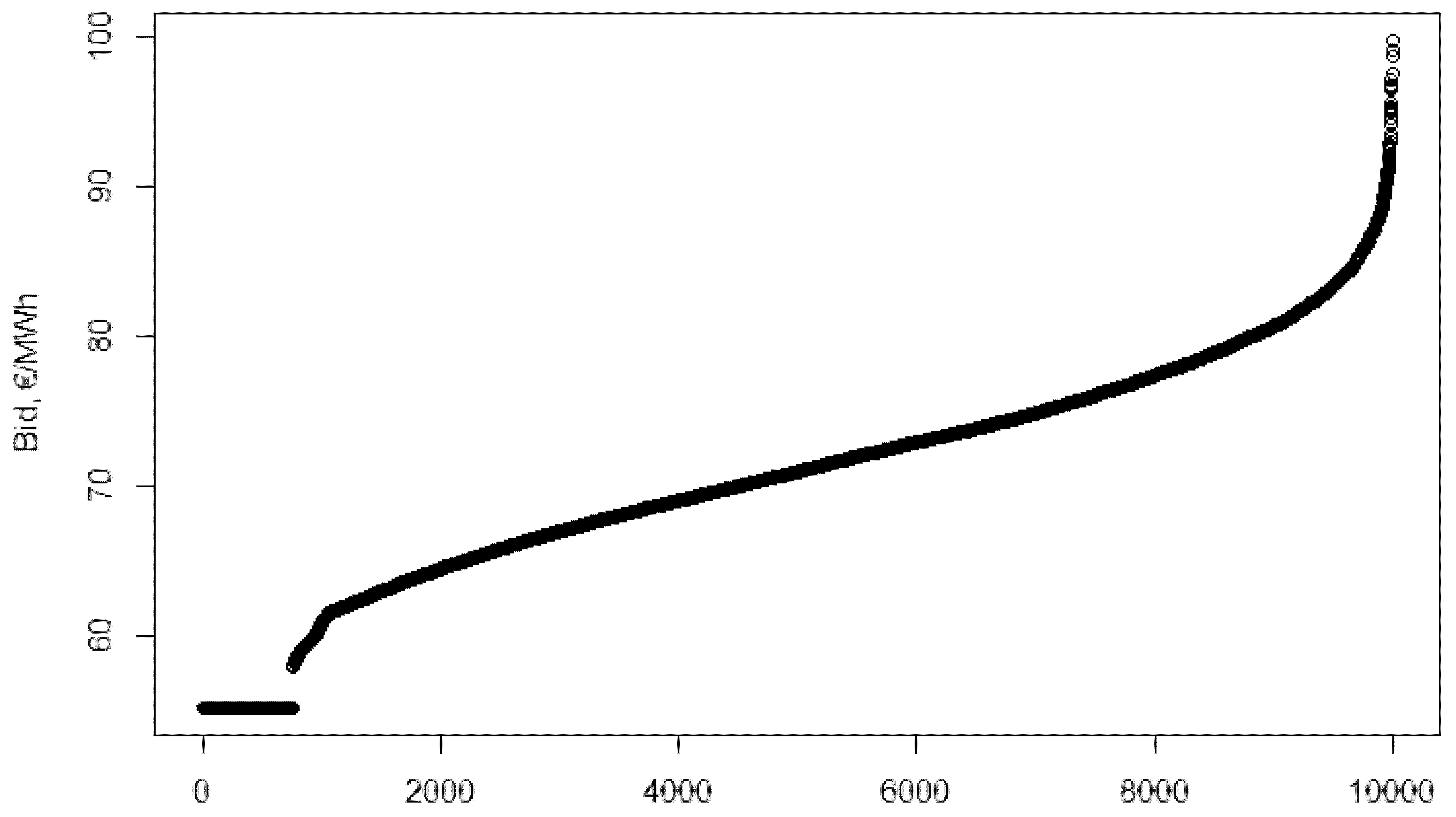
The sorted L C O E values are presented in Figure 5. The first 759 elements are 0, meaning out of 10,000 investment cost simulations 759 are lower than the critical investment cost. For these projects it is assumed that project developers will take part in the auction, since they can make their investment more profitable by winning. This model does not put a cost on participation, so participation is incentivised.

3.2. Nash-Equilibrium Bid Function in Case of the Pay-as-Bid Auction

In the following subsection the algorithm is explained, and results summerised. More details of the calculation, including the code and the data are available as Supplementary Materials.
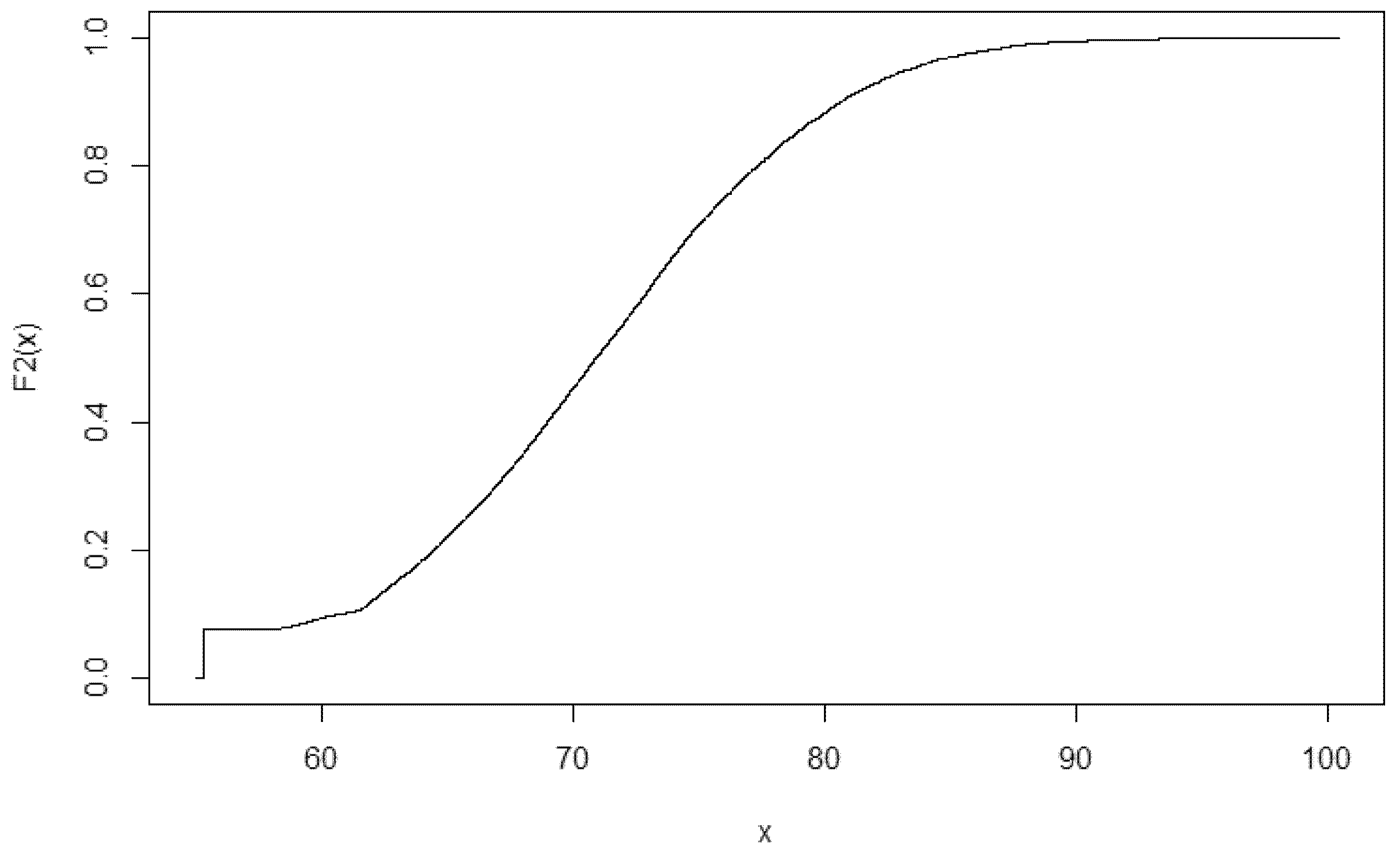
The first step of the iteration assumes a normal distribution for the bids of others, with the mean and variance of the simulated 10,000 L C O E value, of which the cumulative distribution function is F 1 .
Next the optimal bids are calculated for all 10,000 different simulated L C O E values. This way I get 10,000 bids. From the point of view of another participant each of them is equally possible to be the optimal one, as he does not know the exact L C O E , just the possible 10,000 valuations or the valuation distribution.
If this bid distribution is equal to the original, this signals a Nash-equilibrium—though not necessarily the only one—because if all participants assume this bid distribution, then the best response will lead to the assumed distribution making every participants’ bid function the best response to others’. If the two distributions are different, then the optimal bid function—assuming this new distribution—has to be tested in the next step of the iteration.
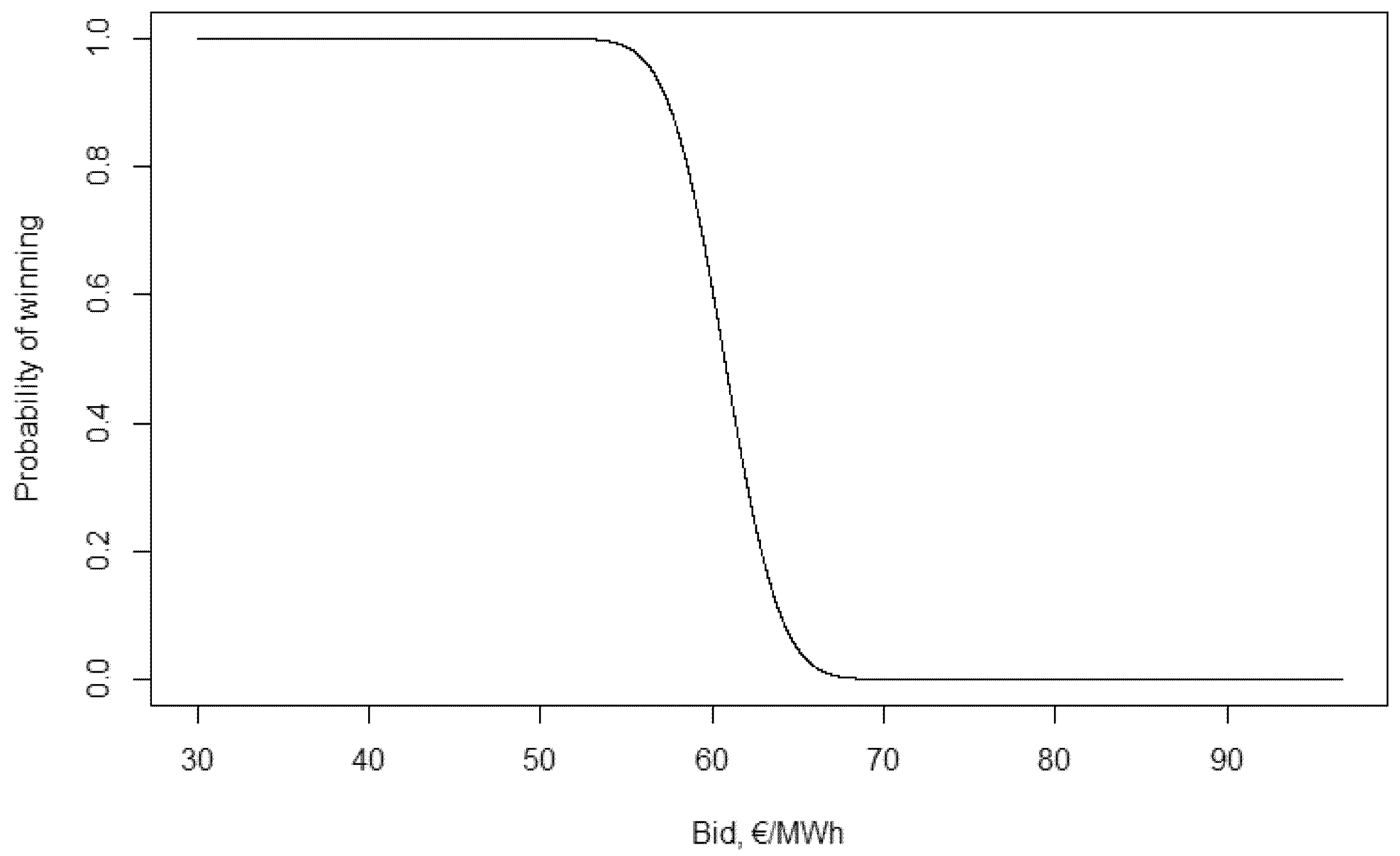
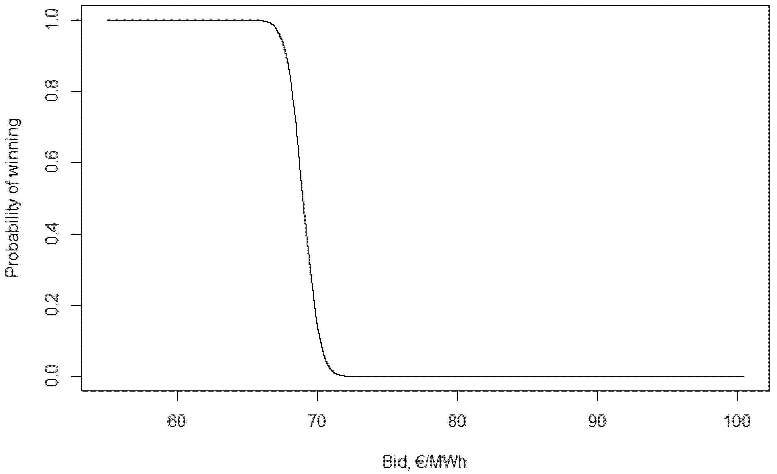
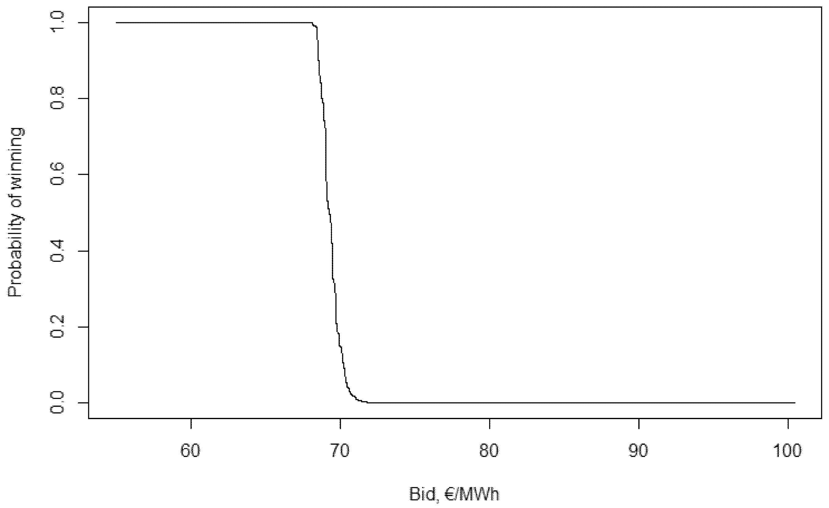
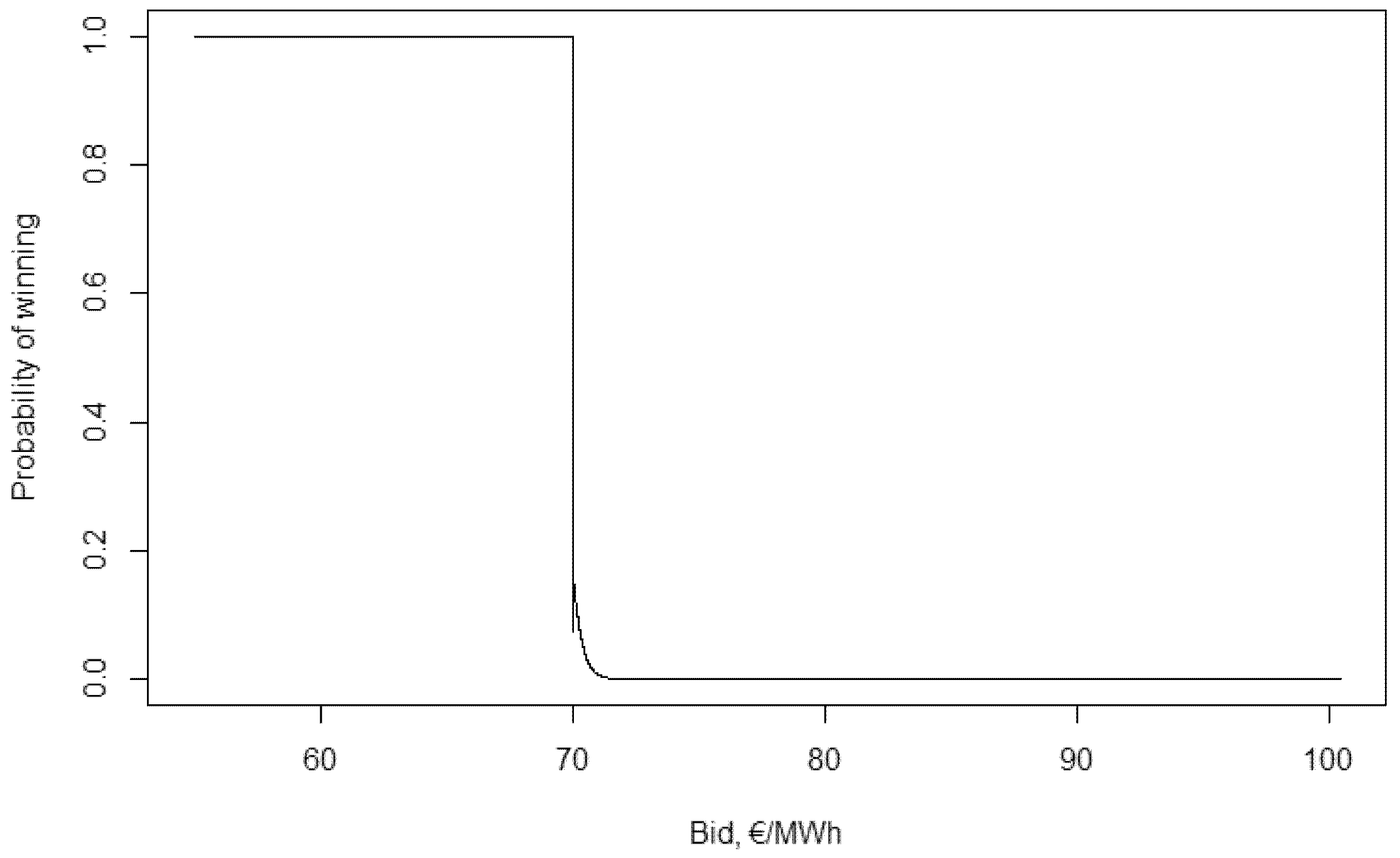
To calculate the optimal bids the probability of winning needs to be calculated for the different bids first. This is shown by figures in Appendix A.
There is a clear range of bids that are “in the game”: with a bid of 50 €/MWh the probability of winning is over 0.9999, while a bid of 70 €/MWh has a probability of winning less than 0.86 × 10 5 . The optimal bid can be calculated for all valuations using these probabilities (for this step I used the command “optimize” of the program R).
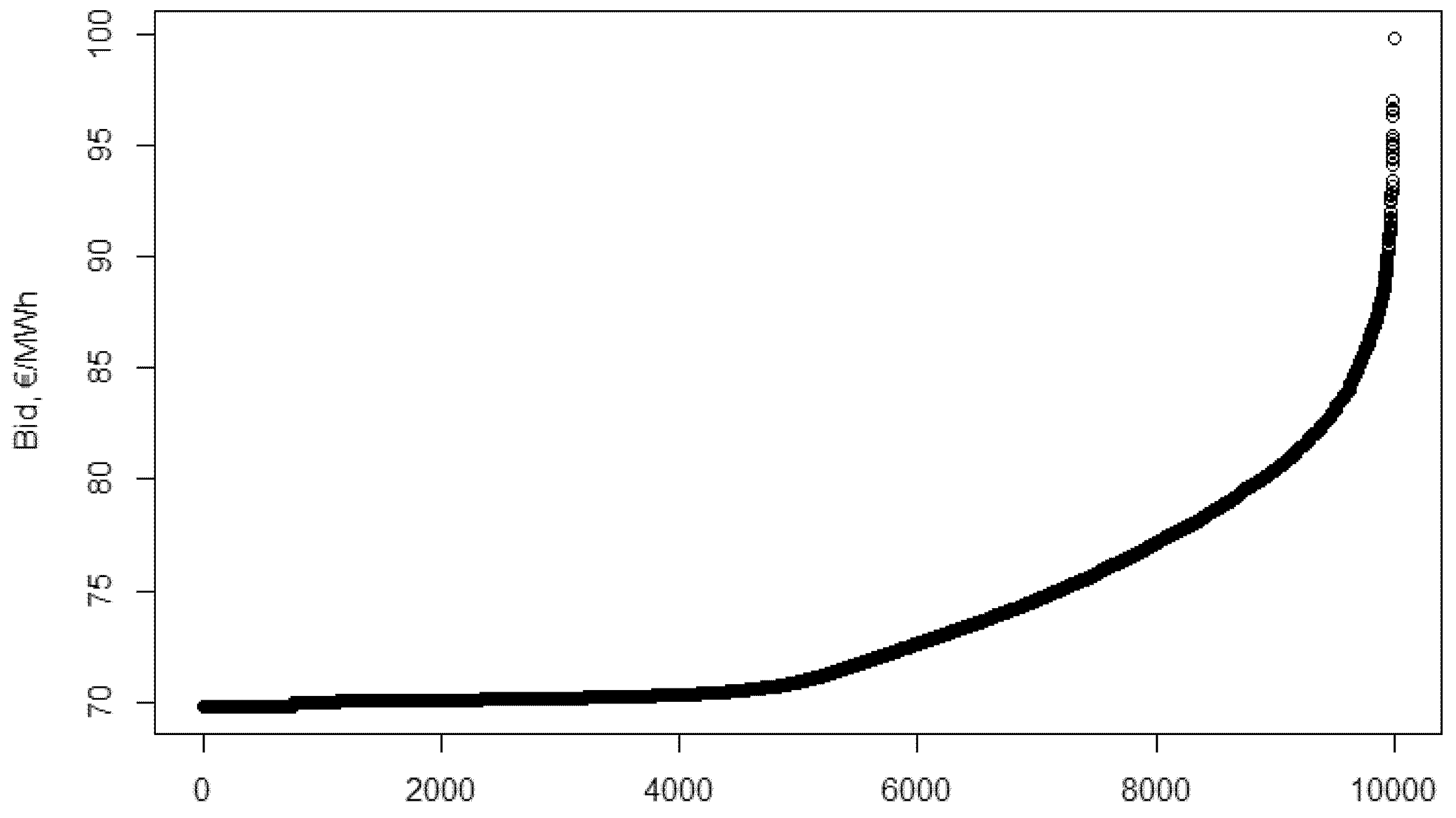
In Figure 6, the optimal bids (y axis) and valuations (x axis) are shown. There is no need to have the exact formula of the bid function at this point, the difference between them is visible from the figures. These are not actual functions at this point—here, the valuation–bid pairs are presented.
To proceed the new bid distribution, F 2 has to be specified. If the optimal bid for all 10,000 possible valuations leads to a distribution F 1 , then it is a Nash-equilibrium. If not, further analysis is needed. It is possible, that the best response would be the same when assuming F 2 as in case of F 1 , but it would mean, the normal bid distribution leads to Nash-equilibrium. Furthermore, as it is shown later, this is not the case.
In order to specify F 2 10,000 optimal bid–valuation pairs had to be fitted. The first step is sorting the optimal bids and depicting them on a graph. We can interpret this graph as the probability of a bid smaller than the y coordinate of a given point is the x coordinate of the given point divided by 10,000. Thus, because of the sorting, the probability of receiving a bid (from this distribution) smaller than the 500th bid is 500 10,000 , while the probability of receiving a bid smaller than the largest bid would be 1 (1 = 10,000 10,000 ).
This way, with some small modifications the inverse of the depicted function will be the cumulative distribution function (from now on referred to as the distribution function). The first modification is that instead of the sequence number (the x coordinate) the ten thousandth of the number is used, to get probabilities.
The first part of the function represented by the horizontal line can not be inverted. The probability of having a bid below the minimum is 0, while the value of the distribution function for bids larger than the minimum bid would also be larger than the one ten thousandth of the highest sequence number of minimum bids (in this case the value of the distribution function will be larger or equal than 759 10,000 for bids larger or equal than the minimum bid, reflecting 759 bids with the minimum value).
The form of this bid distribution comes from the 759 cases out of 10,000 simulated when the L C O E was 0, and without any support the project would be profitable (meaning the expected return can be realised).
The formulas of the distribution functions are included in Appendix A. The distribution function defined above satisfies all conditions to be a distribution function:
F 2 ( x ) = P ( X x ) values   are   between   0   and   1 ,
it   is   monotonically   increasing ,   right-continuous , lim x F 2 ( x ) = 0   and lim x F 2 ( x ) = 1
Having the new assumption for the bid distribution ( F 2 ) the optimal bids can be calculated again. The new optimal bid function then can be compared to the one from Step 1, when assuming F 1 . If these are not equal, then it is not a Nash-equilibrium, as the best response for the others’ assumed optimal bidding strategy is different from the assumed.
As a first step, the probability of winning is calculated for different bids. The new probabilities are “shifted”: with a bid of 65 €/MWh the probability of winning is larger than 0.9999, while it goes down under 1% only at around 76 €/MWh.
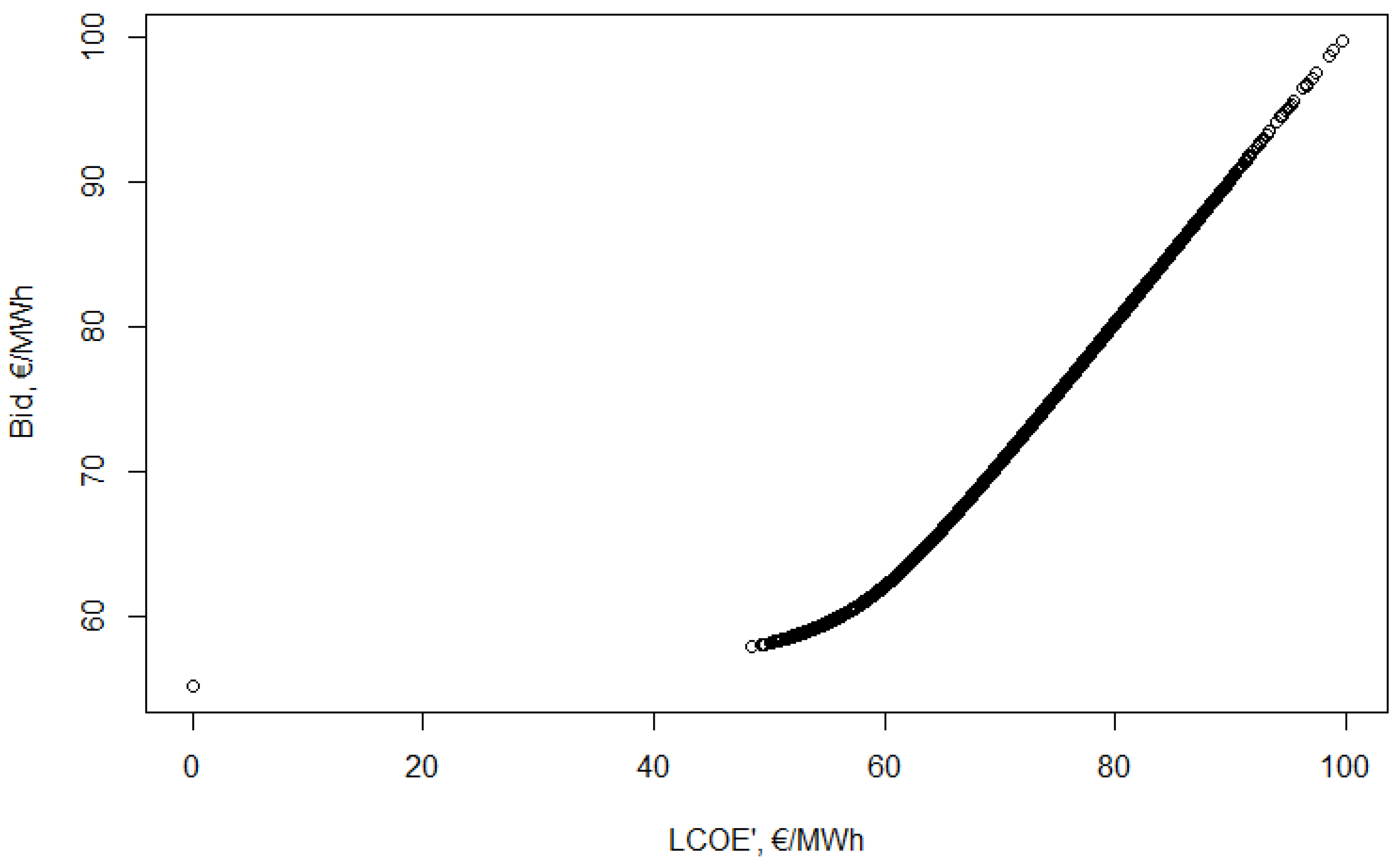
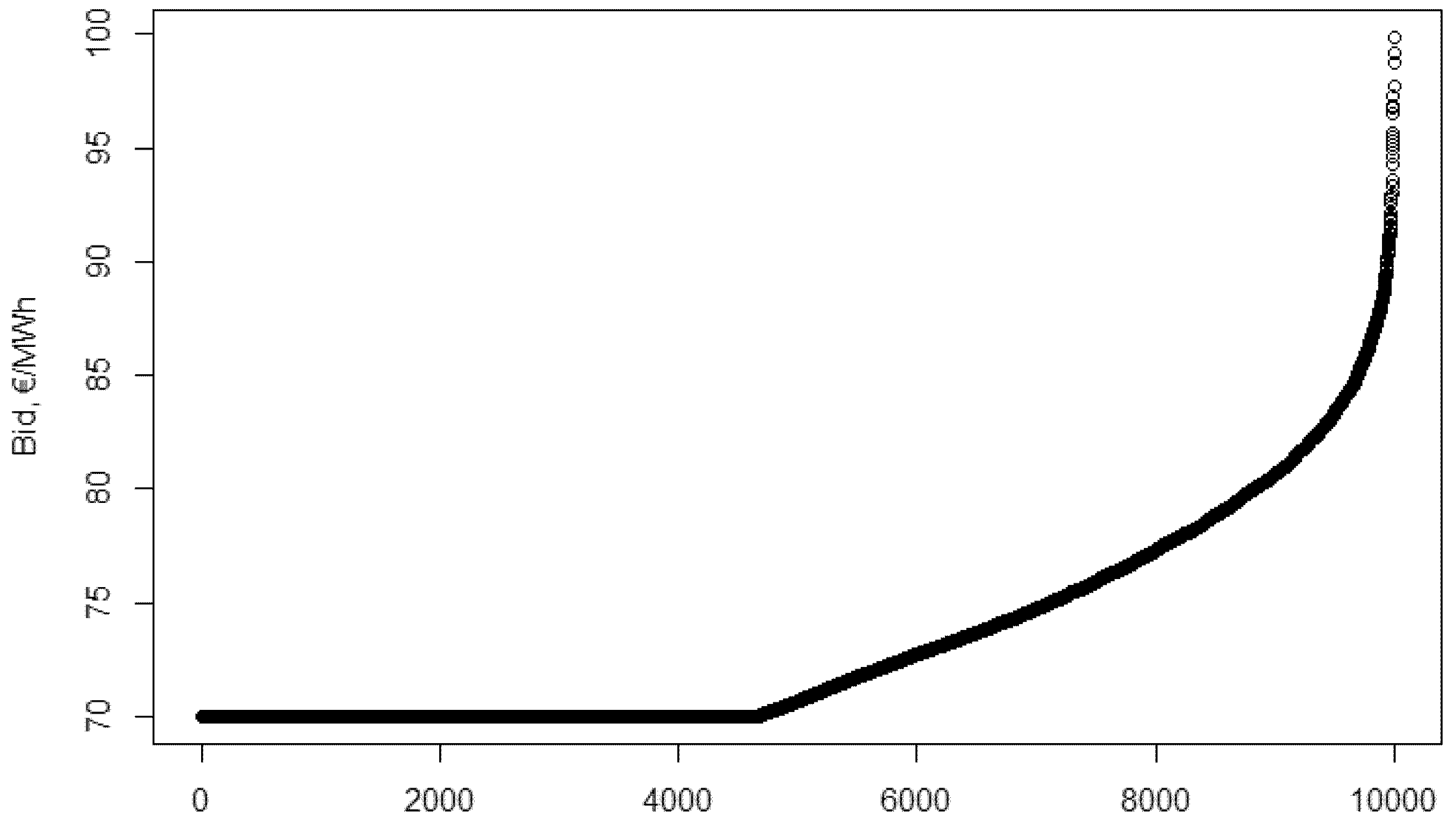
Using these results the optimal bid for the 10,000 different simulated valuations is calculated. The bid function presented on Figure 7 shows a different bid function, so there is another step in the iteration.
The two parts of the function are more distinguishable, with the first part being flatter, then the function becomes steeper. Many participants have the minimum bid, however, this minimum bid is larger than before.
To sum up, the two optimal bid functions are quite different, thus the iteration has to continue, until reaching the Nash-equilibrium.
Next the bid distribution has to be calculated with the help of the bid function, sorting the 10,000 optimal bids for the generated 10,000 valuations. Bids are on average higher than last time, including the maximum bid, and there is a shorter distance between the minimum bid and the next smallest bid. The new bid distribution function, F 3 is presented in Appendix A.
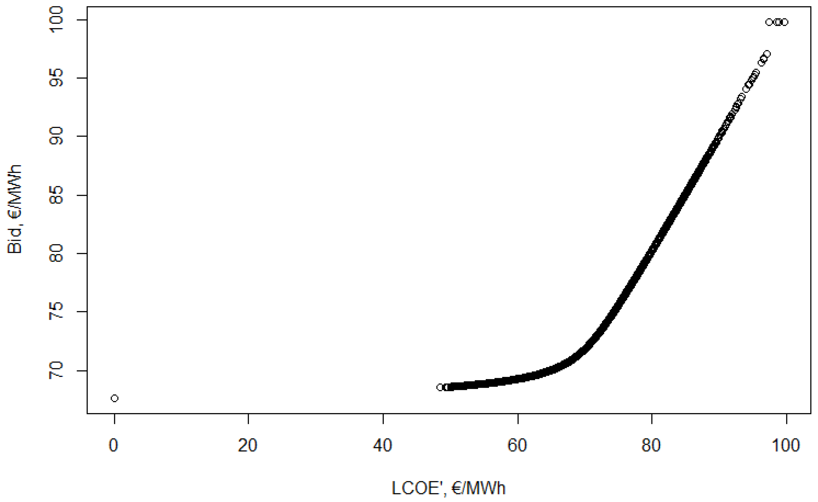
Then the probability of winning for different bids assuming F 3 bid distribution for other participants’ bids is calculated. From this, optimal bids for all 10,000 valuations can be determined.
The first part of the bid function is even flatter, though, still not entirely horizontal, and most bids are very close to 70 €/MWh. The point of inflecion is even clearer before the function turns into a steep, linear trajectory (see details on Figure 8).
After sorting the optimal bids it is clear, that there is no longer a jump between the participants with a 0 valuation and a larger valuation—their bids will be very close to each other. From these sorted bids the new, F 4 bid distribution can be calculated.
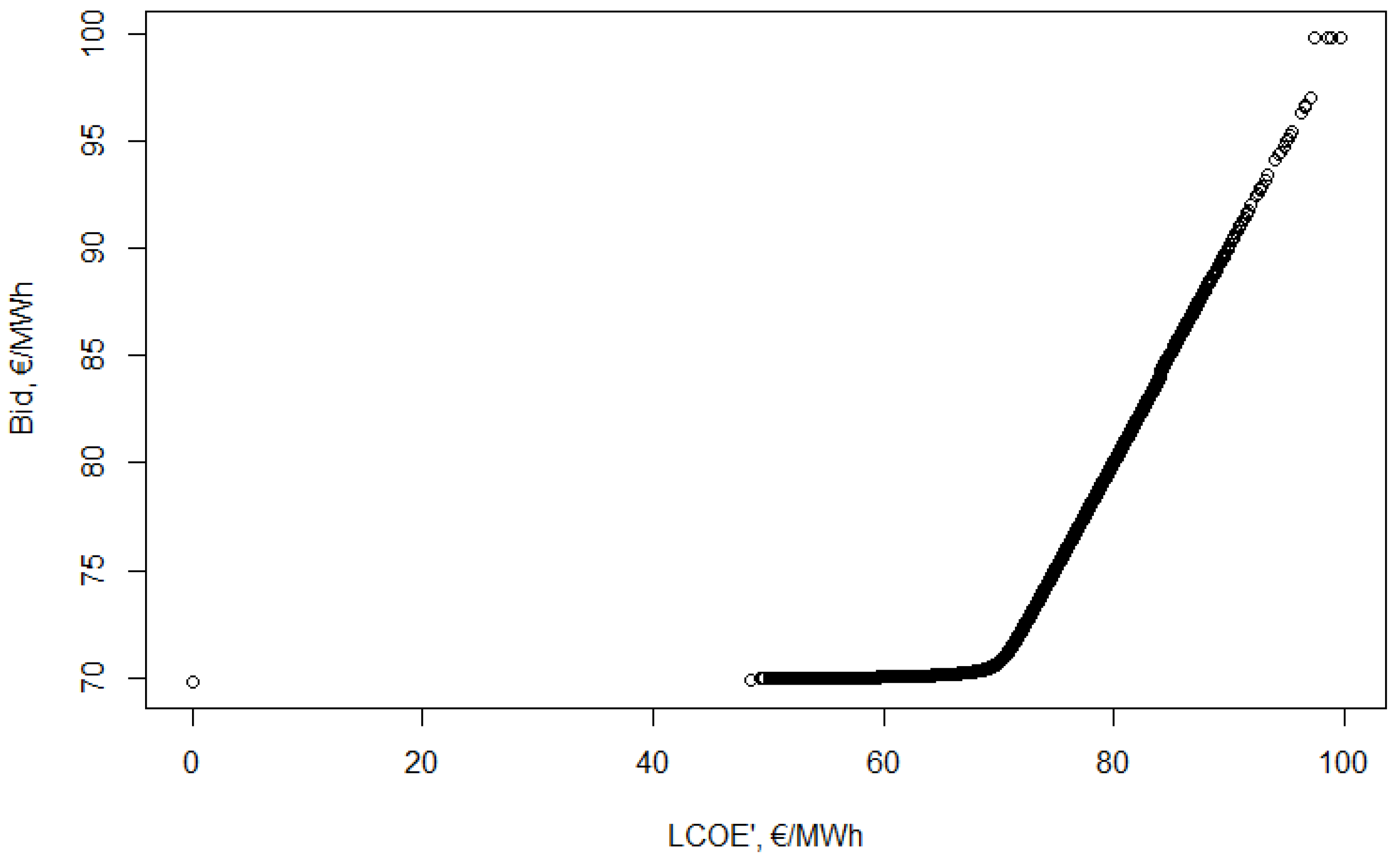
The probability of winning shows that the range, in which the probability is clearly higher than 0 and smaller than 1 gets very narrow. The bid function is quite similar to the one from in Step 3, with only minor differences (see Figure 9). The minimum bids increase from 69.81 to 70.01 €/MWh.
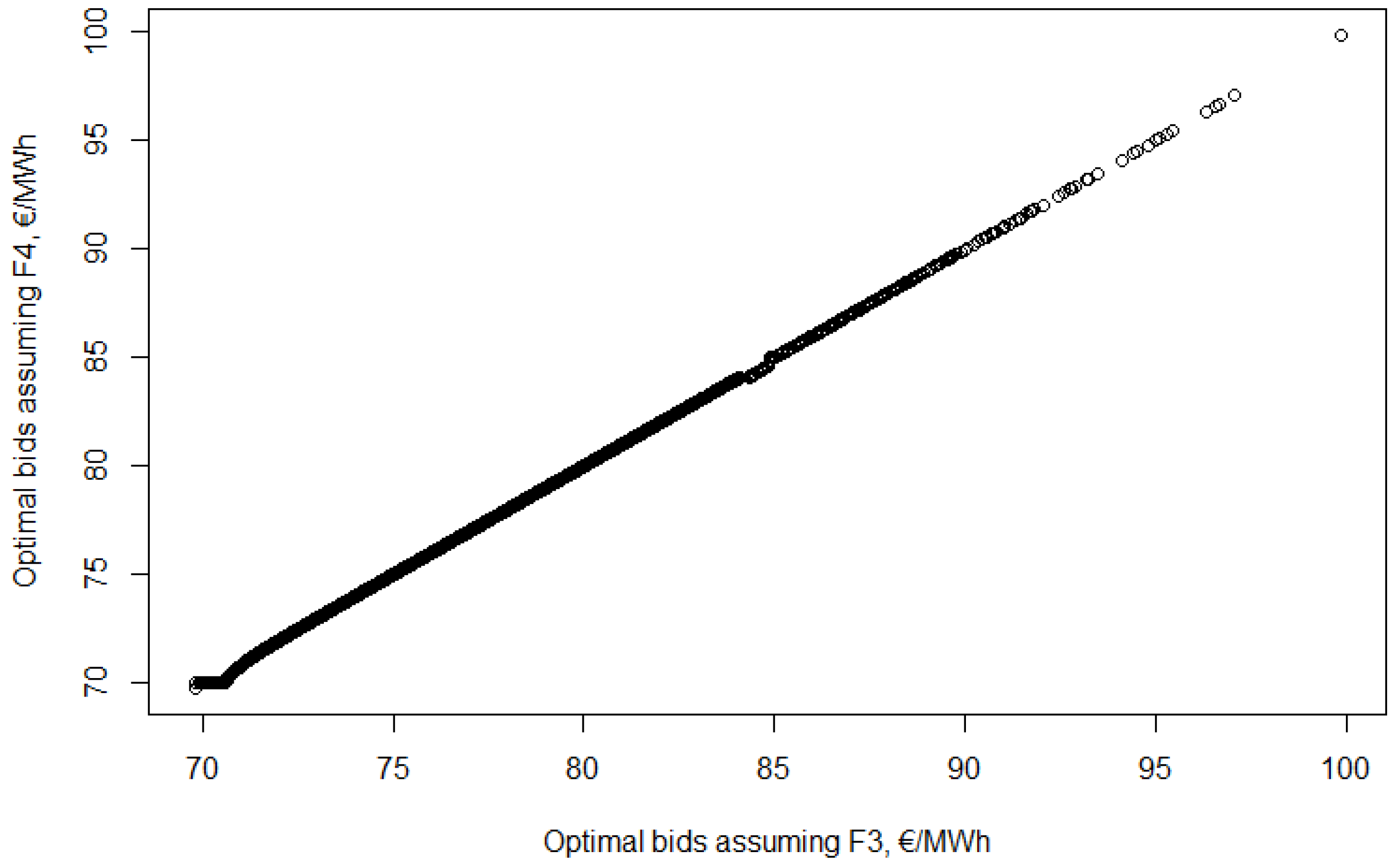
It is likely that this is very close to the Nash-equilibrium. In Figure 10 the magnitude of the difference between the two bid functions is represented. Each valuation is one point, for which the x coordinate is the optimal bid assuming F 3 while the y coordinate is the optimal bid assuming F 4 .
This shows that the two functions are very close to each other and the difference can be found using the Root Mean Square Error (RMSE) value. For the 10,000-item-long series the RMSE value is 0.17 €/MWh. The Normalised Root Mean Square Error (NRMSE) compares this to the mean of the data set—that is 73.39 and 73.45 €/MWh respectively. The NRMSE is less than 0.25% which can be considered rather low. It is close to the point where the iteration stops (0.2%), but it is still higher than that.
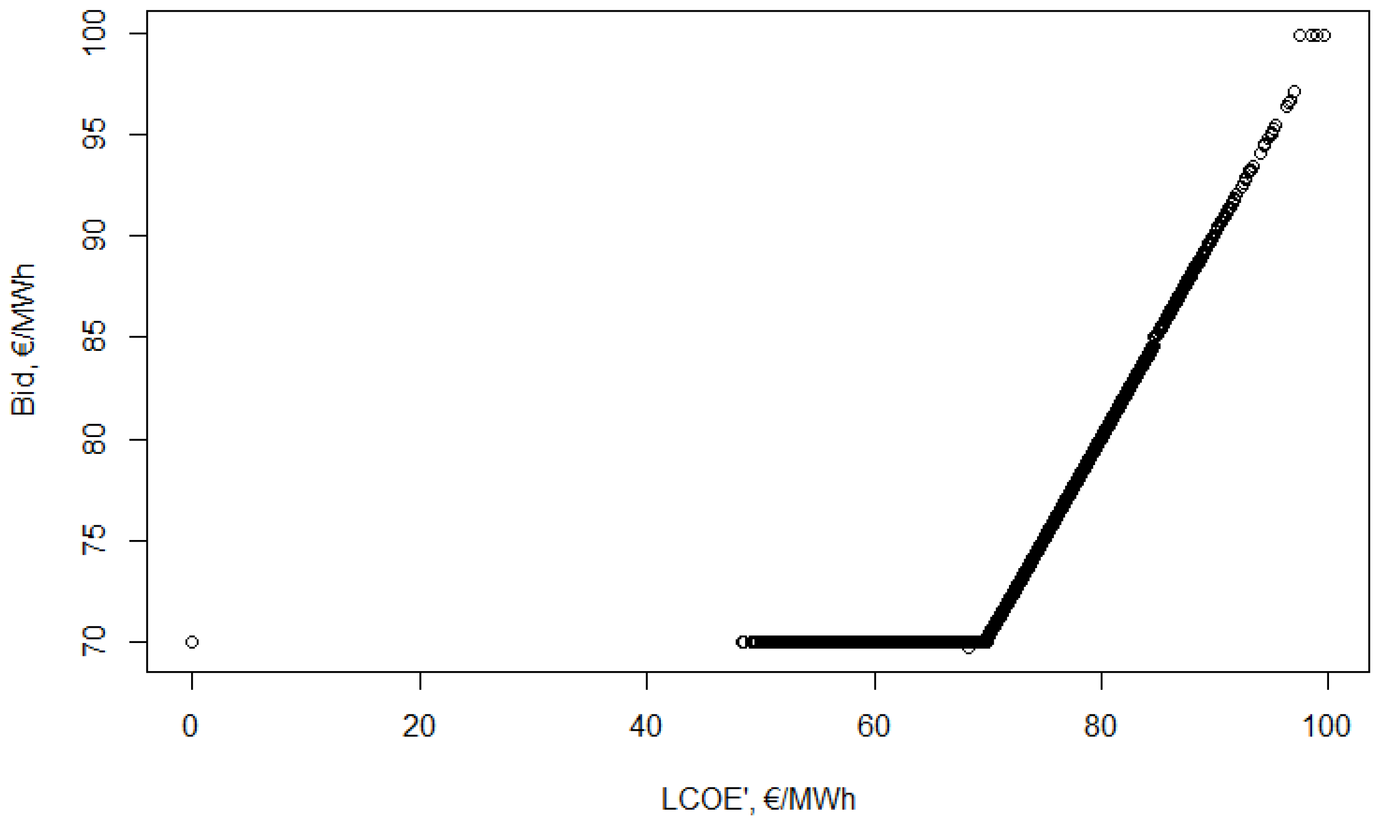
The two bid functions are close enough that it could almost be considered that it is Nash-equilibrium. However, in each step it becomes clear, that the bid functions are getting closer to a specific form: from entirely horizontal to a steepness of around 45 degree.
The following conjecture can be stated: the optimal bid function in a Nash-equilibrium is the following. Under a valuation of 69.706 €/MWh the optimal bid is 70.007 €/MWh, above that the optimal bid is 0.457 €/MWh higher than the 99.78% of the valuation. The exact function form is the following:
f N ( x ) = 70.007 if x < 69.706 0.99779 x + 0.457 if x 69.706 .
The last step is checking whether this is a Nash-equilibrium bidding strategy: assuming this bidding strategy for others would lead to the same optimal bidding strategy.
The first task is calculating the optimal bids assuming f N bid function for all 10,000 valuations, and sorting them. This is presented on Figure A11 in Appendix A.
This shows that these bids are very close to the ones from Step 4—as the definition of the bid function came from these outputs.
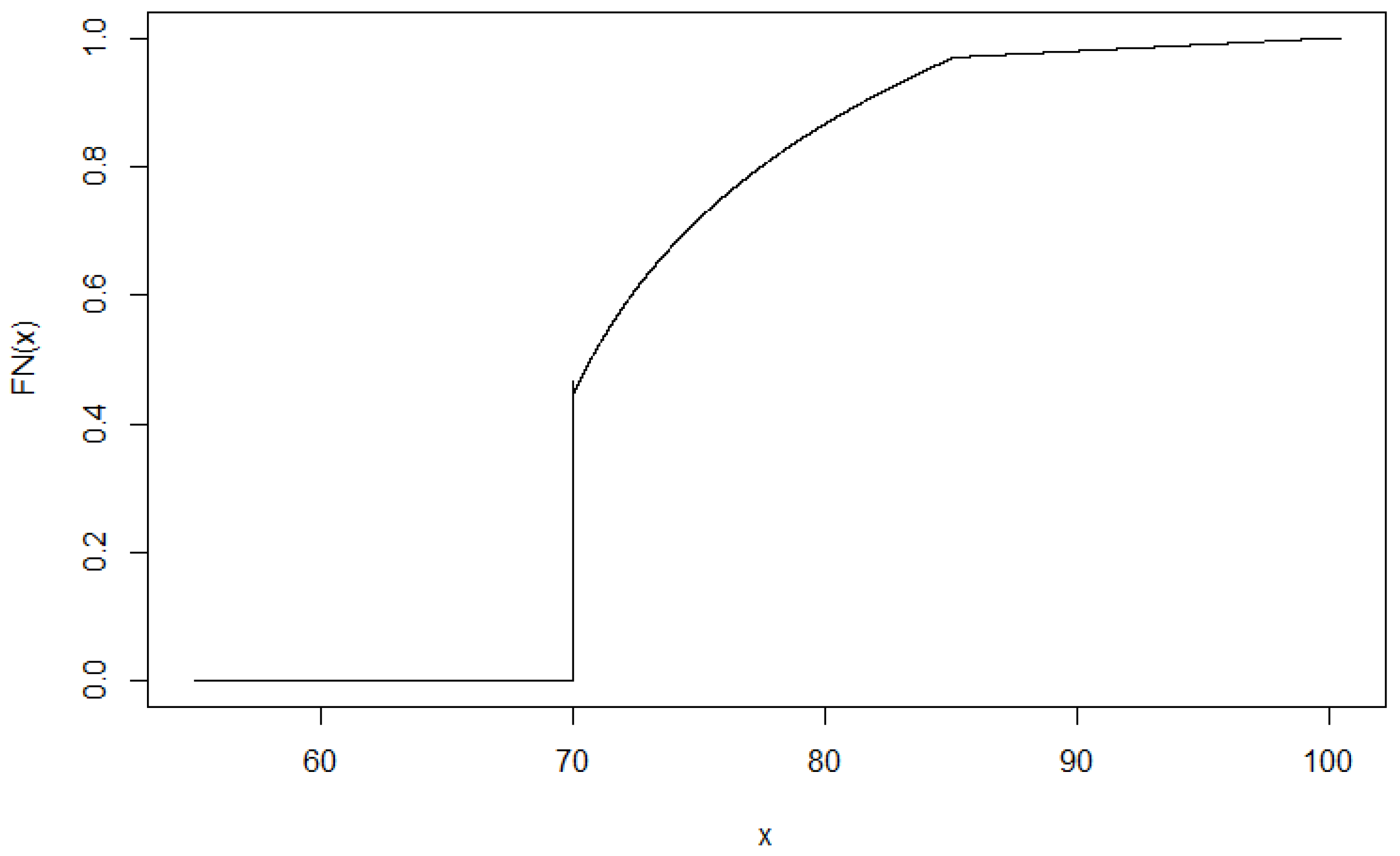
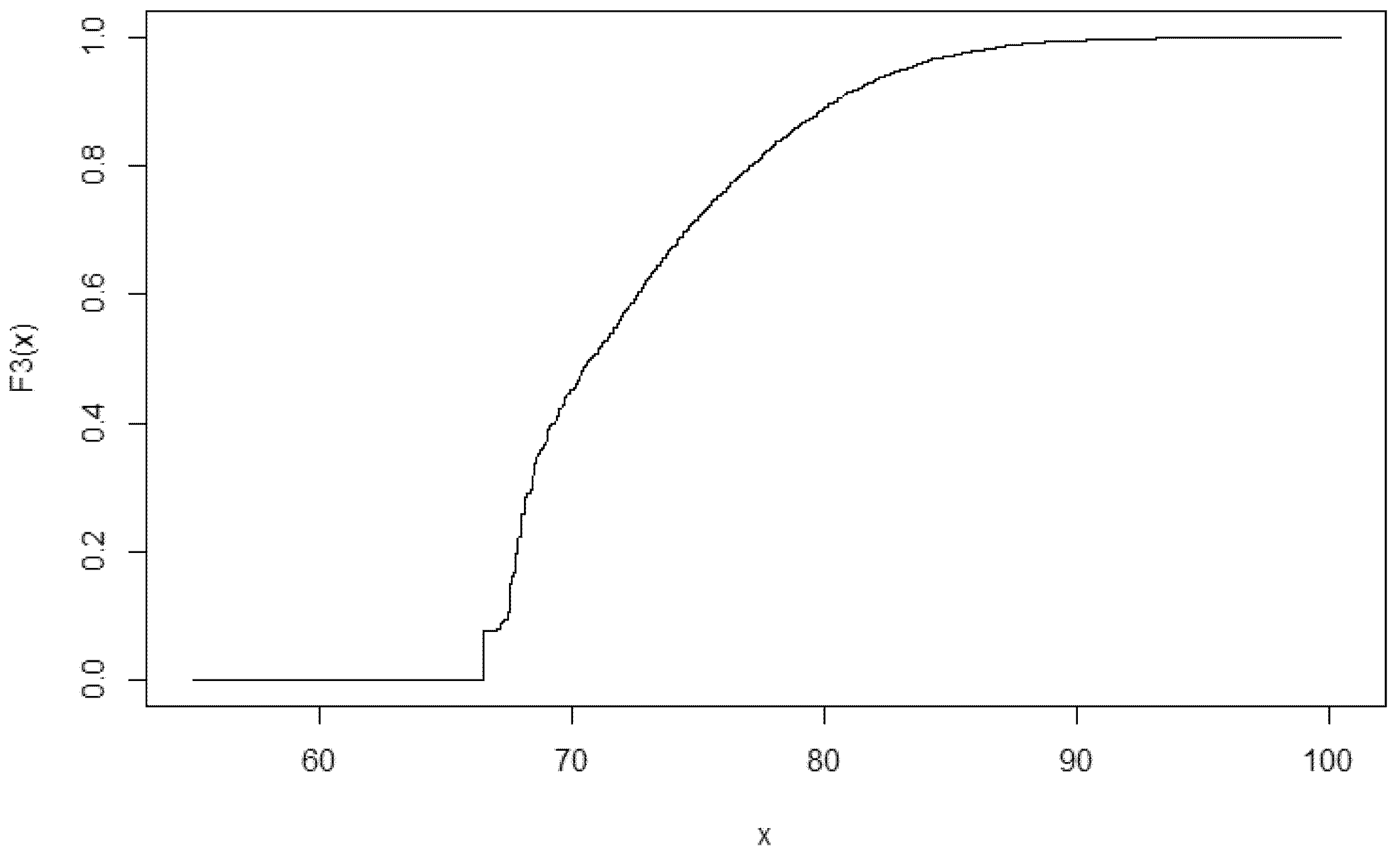
The first part of the function consists of the first 4672 bids: all of them are equal to 70.007 €/MWh. This part of the function can not be inverted, but it is easy to interpret: the probability of other participants’ bids to be less than 70.007 €/MWh is 0, thus F N ( x ) = 0 for all x < 70.007 . The probability of a bid 70.007 €/MWh is exactly 4672 10,000 , so when x 70.007 , then F N ( x ) 4672 10,000 .
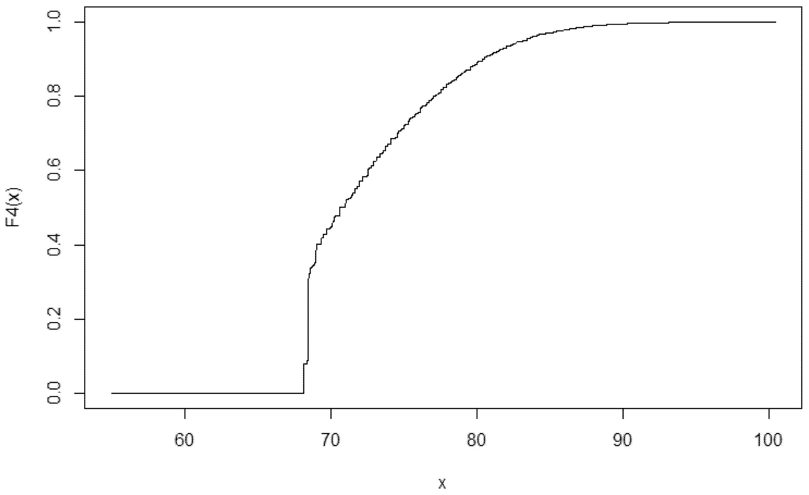
The next section of the function starts from the 4672th smallest bid. Exponential and linear fitting is applied for the rest of the function (the RMSE of the fitted and the original curve is 0.8934. Compared to the mean of the data sets (NRMSE—Normalised Root Mean Square Error) the value is 1.2%). In this step it is rather important to have a precise fitting method when the bid distribution that comes from the assumed bid function is defined. A possible future extension of this work would be to apply a more automatic fitting procedure, that can guarantee to have a well-fitted distribution function in all steps. The new bid distribution can be calculated from the fitted curve. The distribution function F N is presented in Figure 11.
Using this bid distribution the probability of winning and the optimal bids for all valuations can be derived like before. The optimal bid function—assuming the bidding strategy f N for other participants—is presented in Figure 12.
The graph illustrates that the assumed bid function is correct. The assumed and optimal bids for all 10,000 valuations are presented in Figure 13.
To check that the assumed and optimal bidding strategies are the same the (N)RMSE value can be applied: RMSE is 0.10, while NRMSE is 0.15% (mean values are 73.39 and 73.45). This is lower than the pre-defined stopping criterion 0.2%. This means that the two bid functions are very close to each other. From this it can be concluded that the assumed bid function, f N is a Nash-equilibrium bidding strategy: when every other player bids according to this function, then the best response is this function, thus when all players use this bid function it is a Nash-equilibrium.

3.3. Auction Results with the Applied Nash-Equilibrium Bid Functions

In this section the results of the simulation of 100 uniform price and 100 pay-as-bid auctions are presented. To make results more comparable the same 100 × 100 valuations will be used throughout the simulations.
The first step is the simulation of the valuation for all 100 participants. Then, assuming all participants use the Nash-equilibrium bid function all 100 bids can be calculated. The smallest 40 bids are chosen as winners. In case of a tie, winners are chosen randomly. Then the strike price for each winner can be specified, and the total support paid out (or the net present value of it) can be calculated. This again uses own forecast for the electricity prices (the same as assumed when the L C O E is calculated), as this is the best available information.
The results from the two different rules (uniform price and pay-as-bid) are compared according to the smallest and largest winning bid and the total support. They are also compared to the former German PV auctions, taking into account that not all rules could be implemented into this modelling. Since most of the data used for the L C O E calculation is from before 2019, it should be compared with the results from 2017, 2018 and 2019.
As shown on page 12, the Nash-equilibrium bidding strategy is bidding the true valuation under the uniform price rule. Thus, only results of the auction simulation are summarised: the minimum and maximum strike price, and the net present value of the total support.
For each simulation round a valuation “draw” is taken for each of the 100 valuations, using the L C O E distribution (see details above). As these valuations are the bids themselves, they are sorted, then the 40 smallest are selected. The strike price is the 41th smallest bid, this will be received by all winners.
The lowest strike price from the 100 auctions is 65.19 €/MWh, and the highest is 70.86 €/MWh. The mean value of the strike prices is 68.33 €/MWh. These values can be the starting point for comparison to determine how much it costs for the state not to incentivise participants to “tell the truth” about their valuations.
The net present value of the total support to be paid in the next 20 years is calculated using the strike price, the monthly average forecasted (and PV generation weighted) electricity prices and the assumed total generation.
For every month the total support consists of the difference between the strike price and the PV generation weighted average wholesale electricity price (in €/MWh), multiplied by the total generation (in MWh). If it is negative, the total support for that month is 0. The assumed symmetry and uniform price rule lead to all 40 winners receiving the same amount of support, meaning the calculation is only needed for 1 participant, and then multiplied by 40 to arrive at the total support. The net present value of the total support to be paid is the following:
t = 1 20 m = 1 12 [ s t r i k e p r i c e p t m ] + ( 1 + r ) t 40
where, p t m is the PV generation weighted average monthly electricity price in year t and month m, and r is the assumed discount rate.
The minimum support (from the 100 different auction outcomes) is 4.48 million €, and the maximum is 7.16 million €. Out of the 100 auction outcomes the average net present value of support over the next 20 year period is 5.93 million € under the uniform price rule.
For the pay-as-bid auction the most important result is the Nash-equilibrium bid function. According to the literature [1] the participants typically do not tell their true valuations, and ask for more support (or offer less when participants want to buy something on the auction) than their true valuations, which is confirmed by this model.
Figure 12 shows that the participants always bid a higher value than their valuation. With a valuation under 69.706 €/MWh their bid will be 70.007 €/MWh, no matter how much lower their valuation is. This is the Nash-equilibrium bid for players with a valuation of 0 as well. Above that, the optimal bid is 0.457 €/MWh higher than the 99.78% of their valuation.
Several bid values were 70.007 €/MWh, which is surprising considering the mean of the valuations is 65.84 €/MWh (calculating from the 10,000 simulated L C O E values). There are only 18 cases, with a higher strike price than that in the 100 simulated auction rounds together.
To compare the resulting strike prices and support needs with the uniform price case the calculation slightly differs. Each auction has 40 strike prices, where the support level must also be calculated for all 40 winners separately (for all 100 auctions).
i = 1 40 t = 1 20 m = 1 12 [ s t r i k e p r i c e i p t m ] + ( 1 + r ) t
The mean of the support requirement is 6.74 million euros, while the most and least expensive auctions have a cost of 6.75 and 6.74 million euros. This means auction results are quite stable and, more importantly, in most, but not all of the cases, more expensive than the uniform price auctions. The results are summarised in Table 6.
This is an important message for policy makers: according to this model when a group of participants have a 0 valuation (no support is needed for them), and we consider monotone (but not strictly monotone) bid functions, then the uniform price rule (on average) leads to lower support requirements than the pay-as-bid rule, by incentivising participants to bid according to their true valuations. Eventhough this is a special case considering all of the limitations of the model, it is still an interesting and relevant result.
In case of the ordinary auction theory models (assuming bid functions that have an inverse) normally the revenue equivalence theorem stands in most of the cases (see [1]). This means that this work covers a specific different case. Similar results are included in [48], where authors analyse discrete bids and valuations, and arrive to different bid functions compared to the theoretical continuous situation. It is not stated explicitly, but conceivable based on the results, that the revenue equivalence theorem no longer stands in their case neither.
As most of the former models include very different assumptions here the results are compared to the actual German PV auction outcomes. The minimum and maximum strike prices are compared in Table 7.
The results indicate, that the modelled strike prices are rather high comparatively, the only higher prices are observable from the larger (500 MW) auction in March 2019, which can be explained by several factors. It could be a result of own cost calculation not being reflecting precise actual costs. Furthermore, the bid ceiling was not introduced here for the sake of simplicity.
Participants in real life may not calculate the Nash-equilibrium strategies and bid according to them. This is an important limitation of this work, when it comes to policy decisions. However, eventhough the calculation in this specific case is rather complicated, it still can be assumed, that in case of such a large investment the participants are willing to bid according to their best interest.
Unfortunately, we can not compare the difference between the real valuations and the bids, since the information is not publicly available for exact costs of bidders. Only realisation rates of the projects for the first two auctions in 2017 are known, ending up near 100%: 98.85% and 96.74%. This means that the strike price in these auctions were at least as high as the valuation of the bidders.
It should also be emphasised, that in the modelling a typical auction was considered: with 100 participants and 200 MW capacity. The real auctions have similar but not identical attributes. Changing these parameters can also bring some uncertainty regarding the results, a possible future research could answer how robust are them when it comes to different number of participants and winners.
In this model it is a novelty, that investors with 0 support participate in the auctions. With PV cost reduction still underway this can happen in the near future. It is evident, that this situation reveals different bidding behaviour, making the findings of this work important for policy makers. The biggest takeaway is the following: uniform pricing rules might lead to more cost efficient support allocation compared to the pay-as-bid pricing mechanism, through incentivising participants to bid according to their true valuations.

4. Summary and Conclusions

This paper has presented the modelled bidding behaviour on the German PV auctions using the framework of auction theory.
An important theoretical result of this work is the iteration used to find Nash-equilibrium bidding strategies on pay-as-bid auctions. This iteration can be applied to other types of auctions, though the number of steps needed to arrive to Nash-equilibrium can vary considerably. In the observed setting only a few steps are needed.
Beyond the theoretical realm, this work also provides concrete outcomes. The first important numerical results are the L C O E values and their distribution. Accounting for incomes other than support payments results in an interesting L C O E pattern: according to the modified lcoe calculation around 7–8% of all participants do not need any support because their projects will be economical with revenues from the wholesale market. However, it is assumed that they will participate in the auction hoping to receive support.
On the other hand, numerical results are obtained from the simulation of auctions. Based on the information about the former PV auctions in Germany 100 participants and a 5 MW project are assumed for everyone. The total supported amount is 200 MW, leaving 40 winners. With a technology specific auction, symmetry can be assumed.
Following literature for the uniform price auctions all players bid according to their true valuations. The support levels emerging from the 100 simulations vary between 65.19 and 70.86 €/MWh, while the average strike price is 68.33 €/MWh. The total average support expenditure (calculating the net present value for the whole support period) is around 5.93 million euro (all values are calculated in 2019 euros).
The results are telling for the pay-as-bid rule. The Nash-equilibrium bidding strategy with a valuation under 69.706 €/MWh is 70.007 €/MWh. Above that, the optimal bid is 0.457 €/MWh higher than 99.78% of the valuation. This bid function can be explained mostly by the relatively large number of participants with 0 support need.
The expected value of the valuation of participants is 65.8 €/MWh with a significant number of participants having a lower than 70.007 €/MWh valuation in each simulated round. Across all 100 simulated auctions the highest winning bid is 70.90 €/MWh, and the lowest is 70.007 €/MWh. Consequently, the net present value of the total support expenditure is much higher, around 6.74 million euro.
These results come from a model that is based on the specific German PV auction rules, however technology specific (thus basically symmetric) pay-as-bid auctions, with capacity constraints are organised in several other countries including Greece, Spain and Portugal. The actual auction results, and the form of the bid function or the number of steps needed in the iteration can serve as a benchmark for other countries as well.
Possible future research directions might include the application of the model and the iteration to other countries with similar auction designs, or for other technologies (e.g., wind). The sensitivity of the iteration (the resulting bid function and the number of steps needed to arrive there) might be tested to the starting valuation and bid distribution assumption, the number of participants, and winners. A wider research endeavour might also attempt to provide conditions for convergence in the iteration algorithm.

Supplementary Materials

The R code of the entire calculation and the data regarding electricity price forecast and production are available online at https://www.mdpi.com/1996-1073/14/2/516/s1.

Funding

This research received no external funding.

Institutional Review Board Statement

Not applicable.

Informed Consent Statement

Not applicable.

Acknowledgments

I would like to thank the continuous support of Gyula Magyarkuti throughout my entire PhD research. I would also like to thank Gábor Virág and András Kiss for their valuable comments and discussions. The work could not be carried out without the SEERMAP project, I would like to thank the work of László Szabó, András Mezősi, Zsuzsanna Pató, Ágnes Kelemen, Gustav Resch and Lukas Liebmann.

Conflicts of Interest

The author declares no conflict of interest.

Appendix A. Figures and Distribution Functions in the Different Iteration Steps

Figure A1. Probability of winning in case of different bids, assuming F 1 bid distribution, source: own figure.
Energies 14 00516 g0a1
Figure A2. Sorted optimal bids, assuming F 1 bid distribution, source: own figure.
Energies 14 00516 g0a2
Figure A3. The F 2 bid distribution, source: own figure.
Energies 14 00516 g0a3
Figure A4. Probability of winning in case of different bids, assuming F 2 bid distribution, source: own figure.
Energies 14 00516 g0a4
Figure A5. Sorted optimal bids, assuming F 2 bid distribution, source: own figure.
Energies 14 00516 g0a5
Figure A6. The F 3 bid distribution, source: own figure.
Energies 14 00516 g0a6
Figure A7. Probability of winning in case of different bids, assuming F 3 bid distribution, source: own figure.
Energies 14 00516 g0a7
Figure A8. Sorted optimal bids, assuming F 3 bid distribution, source: own figure.
Energies 14 00516 g0a8
Figure A9. The F 4 bid distribution, source: own figure.
Energies 14 00516 g0a9
Figure A10. Probability of winning in case of different bids, assuming F 4 bid distribution, source: own figure.
Energies 14 00516 g0a10
Figure A11. Sorted optimal bids assuming f N bid function, source: own figure.
Energies 14 00516 g0a11
Figure A12. Probability of winning in case of different bids, assuming F N bid distribution, source: own figure.
Energies 14 00516 g0a12
F 2 ( x ) = 0 if x < 55.17 759 10000 if 55.17 x < 55.17 + 10 ( 10 ) 759 10000 + ( x 55.17 ) 1060 759 10000 61.46 55.17 if 55.17 + 10 ( 10 ) x < 61.46 1060 10000 + ( x 61.46 ) 9975 1060 10000 92.52 61.46 if 61.46 x < 92.52 9975 10000 + ( x 92.52 ) 10000 9975 10000 99.77 92.52 if 92.52 x < 99.77 1 if x 99.77 .
F 3 ( x ) = 0 if x < 67.65 759 10000 if 67.65 x < 67.65 + 10 ( 10 ) 759 10000 + ( x 67.65 ) 1060 759 10000 69.19 67.65 if 67.65 + 10 ( 10 ) x < 69.19 ln ( x 67.70 ) 0.00029 10000 if 69.19 x < 84.21 9629 10000 + ( x 84.21 ) 10000 9629 10000 99.79 84.21 if 84.21 x < 99.79 1 if x 99.79
F 4 ( x ) = 0 if x < 69.81 759 10000 if 69.81 x < 69.81 + 10 ( 10 ) 759 10000 + ( x 69.81 ) 1060 759 10000 70.007 69.81 if 69.81 + 10 ( 10 ) x < 70.007 ln ( x 66.26 ) 0.00030 10000 if 70.007 x < 85.04 9700 10000 + ( x 85.04 ) 10000 9700 10000 99.84 85.04 if 85.04 x < 99.84 1 if x 99.84
F N ( x ) = 0 if x < 70.007 4672 10000 if 70.007 x < 70.009 + 10 ( 10 ) ln ( x 66.19 ) 0.00030 10000 if 70.009 + 10 ( 10 ) x < 85.17 9706 10000 + ( x 85.17 ) 10000 9706 10000 99.84 85.17 if 85.17 x < 99.84 1 if x 99.84

References

  1. Krishna, V. Auction Theory, 2nd ed.; Bentley, S., Ed.; Academic Press: London, UK, 2010. [Google Scholar]
  2. European Commission Directive 2009/28/EC of the European Parliament and of the Council of 23 April 2009 on the Promotion of the Use of Energy from Renewable Sources and Amending and Subsequently Repealing Directives 2001/77/EC and 2003/30/EC, 23.04.2009. Available online: https://eur-lex.europa.eu/legal-content/EN/ALL/?uri=CELEX%3A32009L0028 (accessed on 25 May 2019).
  3. European Council Conclusions—23/24 October 2014. Available online: https://www.consilium.europa.eu/uedocs/cms_data/docs/pressdata/en/ec/145397.pdf (accessed on 25 May 2019).
  4. Blücher, F.; von Gephart, M.; Wigand, F.; Anatolitis, V.; Winkler, J.; Held, A.; Sekamane, J.K.; Kitzing, L. AURES II Report D6.1, Design Options for Cross-Border Auctions. 2018. Available online: http://aures2project.eu/wp-content/uploads/2019/06/AURES_II_D6_1_final.pdf (accessed on 2 October 2019).
  5. Eurostat SHARES Database. 2020. Available online: https://ec.europa.eu/eurostat/web/energy/data/shares (accessed on 4 January 2021).
  6. European Commission Guidelines on State Aid for Environmental Protection and Energy 2014–2020, OJ C 200, 28.6.2014. Available online: https://eur-lex.europa.eu/legal-content/EN/TXT/?uri=CELEX%3A52014XC0628%2801%29 (accessed on 25 May 2019).
  7. Wigand, F.; Förster, S.; Amazo, A.; Tiedemann, S. AURES Report D4.2, Auctions for Renewable Energy Support: Lessons Learnt from International Experiences. 2016. Available online: http://auresproject.eu/sites/aures.eu/files/media/documents/aures_wp4_synthesis_report.pdf (accessed on 25 May 2019).
  8. Del Río, P. AURES Report D4.4-ZM, Auctions for Renewable Support in Zambia: Instruments and Lessons Learnt. 2017. Available online: http://auresproject.eu/sites/aures.eu/files/media/documents/zambia_final.pdf (accessed on 25 May 2019).
  9. Del Río, P. AURES Report D4.4-PE, Auctions for Renewable Support in Peru: Instruments and Lessons Learnt. 2017. Available online: http://auresproject.eu/sites/aures.eu/files/media/documents/peru_final.pdf (accessed on 25 May 2019).
  10. Cretu, G. RES Auctions in the Energy Community. In Proceedings of the 2nd AURES II Regional Workshop Renewable Energy Auctions in Austria—Best Practices and Impact Mitigation, Vienna, Austria, 22 November 2019. [Google Scholar]
  11. Fraunhofer Energy Charts Database, Net Installed Electricity Generation Capacity in Germany. Available online: https://www.energy-charts.de/power_inst.htm (accessed on 2 October 2019).
  12. Klemperer, P. Auction Theory: A guide to the literature, Oxford University Economics Working Paper No. 1999-W12. J. Econ. Surv. 1999, 13, 227–286. [Google Scholar] [CrossRef]
  13. Milgrom, P.R.; Weber, R.J. A Theory of Auctions and Competitive Bidding. Econometrica 1982, 50, 1089–1122. Available online: http://www.jstor.org/stable/1911865?origin=crossref (accessed on 17 May 2019). [CrossRef]
  14. Morgan, J. Efficiency in auctions: Theory and practice. J. Int. Money Financ. 2001, 20, 809–838. [Google Scholar] [CrossRef]
  15. Hailu, A.; Thoyer, S. Multi-unit auction format design. J. Econ. Interact. Coordinat. 2006, 1, 129–146. [Google Scholar] [CrossRef]
  16. De Keijzer, B.; Markakis, E.; Schäfer, G.; Telelis, O. Inefficiency of standard multi-unit auctions. In Proceedings of the 21st Annual European Symposium, Sophia Antipolis, France, 2–4 September 2013; Springer: Berlin/Heidelberg, Germany, 2013; pp. 385–396. [Google Scholar]
  17. Hudson, R. Analysis of Uniform and Discriminatory Price Auctions in Restructured Electricity Markets; Oak Ridge National Laboratory: Oak Ridge, TN, USA, 2000. [Google Scholar]
  18. Federico, G.; Rahman, D. Bidding in an electricity pay-as-bid auction. J. Regul. Econ. 2003, 24, 175–211. [Google Scholar] [CrossRef]
  19. Tierney, S.F.; Schatzki, T.; Mukerji, R. Uniform-Pricing Versus Pay-as-Bid in Wholesale Electricity Markets: Does it Make a Difference? ISO New York: New York, NY, USA, 2008. [Google Scholar]
  20. Sugianto, L.F.; Liao, K.Z. Comparison of different auction pricing rules in the electricity market. Modern Appl. Sci. 2014, 8, 147. [Google Scholar] [CrossRef]
  21. Reiley, D.H. Field experiments on the effects of reserve prices in auctions: More magic on the internet. RAND J. Econ. 2006, 37, 195–211. Available online: https://onlinelibrary.wiley.com/doi/epdf/10.1111/j.1756-2171.2006.tb00012.x (accessed on 17 May 2019). [CrossRef] [Green Version]
  22. Ostrovsky, M.; Schwarz, M. Reserve prices in internet advertising auctions: A field experiment. EC 2011, 11, 59–60. Available online: https://web.stanford.edu/~ost/papers/rp.pdf (accessed on 17 May 2019).
  23. McAfee, R.P.; McMillan, J. Auctions and bidding. J. Econ. Lit. 1987, 25, 699–738. [Google Scholar]
  24. Del Río, P.; Linares, P. Back to the future? Rethinking auctions for renewable electricity support. Renew. Sustain. Energy Rev. 2014, 35, 42–56. [Google Scholar] [CrossRef] [Green Version]
  25. Shrimali, G.; Konda, C.; Farooquee, A.A. Designing renewable energy auctions for India: Managing risks to maximize deployment and cost-effectiveness. Renew. Energy 2016, 97, 656–670. [Google Scholar] [CrossRef]
  26. Atalay, Y.; Kalfagianni, A.; Pattberg, P. Renewable energy support mechanisms in the Gulf Cooperation Council states: Analyzing the feasibility of feed-in tariffs and auction mechanisms. Renew. Sustain. Energy Rev. 2017, 72, 723–733. [Google Scholar] [CrossRef]
  27. Haufe, M.C.; Ehrhart, K.M. Auctions for renewable energy support–Suitability, design, and first lessons learned. Energy Policy 2018, 121, 217–224. [Google Scholar] [CrossRef]
  28. Kylili, A.; Fokaides, P.A. Competitive auction mechanisms for the promotion renewable energy technologies: The case of the 50 MW photovoltaics projects in Cyprus. Renew. Sustain. Energy Rev. 2015, 42, 226–233. [Google Scholar] [CrossRef]
  29. Güth, W.; Ivanova-Stenzel, R.; Wolfstetter, E. Wolfstetter Bidding Behavior in Asymmetric Auctions: An Experimental Study. Eur. Econ. Rev. 2005, 49, 1891–1913. [Google Scholar] [CrossRef] [Green Version]
  30. Kreiss, J.; Ehrhart, K.; Haufe, M. Appropriate design of auctions for renewable energy support—Prequalifications and penalties. Energy Policy 2017, 101, 512–520. [Google Scholar] [CrossRef]
  31. Iychettira, K.; Hakvoort, R.; Linares, P. Towards a comprehensive policy for electricity from renewable energy: An approach for policy design. Energy Policy 2017, 10, 169–182. [Google Scholar] [CrossRef]
  32. Anatolitis, V.; Welisch, M. Putting renewable energy auctions into action–An agent-based model of onshore wind power auctions in Germany. Energy Policy 2017, 110, 394–402. [Google Scholar] [CrossRef]
  33. Anatolitis, V. Simulation of Onshore Wind Power Auctions in Germany Considering Different Auction Designs—An Agent Based Model. Master’s Thesis, Karlsruhe Institute of Technology and Technical University of Vienna, Vienna, Austria, 2016. [Google Scholar]
  34. Fraunhofer Levelized Cost of Electricity, Renewable Energy Technologies, March 2018. Available online: https://www.ise.fraunhofer.de/en/publications/studies/cost-of-electricity.html (accessed on 25 May 2019).
  35. Fraunhofer Current and Future Cost of Photovoltaics. Long-Term Scenarios for Market Development, System Prices and LCOE of Utility-Scale PV Systems. Study on Behalf of Agora Energiewende. Available online: https://www.ise.fraunhofer.de/content/dam/ise/de/documents/publications/studies/AgoraEnergiewende_Current_and_Future_Cost_of_PV_Feb2015_web.pdf (accessed on 25 May 2019).
  36. Lazard Lazard’s Levelized Cost of Energy Analysis—Version 11.0. Available online: https://www.lazard.com/media/450337/lazard-levelized-cost-of-energy-version-110.pdf (accessed on 26 May 2019).
  37. IEA Renewables 2017, Analysis and Forecasts to 2022. Available online: https://www.iea.org/renewables2017/ (accessed on 26 May 2019).
  38. IRENA Renewable Power Generation Costs in 2017. Available online: http://www.irena.org/publications/2018/Jan/Renewable-power-generation-costs-in-2017 (accessed on 26 May 2019).
  39. Mezősi, A.; Szabó, L. Model based evaluation of electricity network investments in Central Eastern Europe. Energy Strategy Rev. 2016, 13, 53–66. [Google Scholar] [CrossRef]
  40. ENTSO-E Transparency Platform. Available online: https://transparency.entsoe.eu/ (accessed on 1 March 2018).
  41. Klobasa, M.; Ragwitz, M. Diskussionspapier Contract for Difference Regime (CfD)—Mo Gliche Ausgestaltungen, Karlsruhe, Fraunhofer. 2018. [Google Scholar]
  42. Szabó, L.; Mezősi, A.; Pató, Z.; Kelemen, Á.; Beöthy, Á.; Kácsor, E.; Kaderják, P.; Resch, G.; Liebmann, L.; Hiesl, A.; et al. South East Europe Electricity Roadmap: Regional Report: South East Europe, Budapest, Hungary: REKK Regionális Energia- és Infrastruktúra-Politikai Együttműködésért Alapítvány. 2017, p. 64. Available online: https://rekk.hu/downloads/projects/SEERMAP_RR_SEE_A4_ONLINE.pdf (accessed on 2 February 2020).
  43. Szabó, L.; Kelemen, Á.; Mezősi, A.; Pató, Z.; Kácsor, E.; Resch, G.; Liebmann, L. South East Europe electricity roadmap–modelling energy transition in the electricity sectors. Clim. Policy 2019, 19, 495–510. [Google Scholar] [CrossRef] [Green Version]
  44. Bundesnetzagentur Ausschreibungen 2019, Statistics about PV Auctions. Available online: https://www.bundesnetzagentur.de/DE/Sachgebiete/ElektrizitaetundGas/Unternehmen_Institutionen/Ausschreibungen/Solaranlagen/BeendeteAusschreibungen/BeendeteAusschreibungen_node.html (accessed on 3 October 2020).
  45. Higgins, N.A. Computational and Experimental Market Design. Ph.D. Thesis, University of Maryland, College Park, MD, USA, 2010. Available online: https://drum.lib.umd.edu/handle/1903/10260 (accessed on 5 January 2020).
  46. Marshall, R.C.; Meurer, M.J.; Richard, J.F.; Stromquist, W. Numerical analysis of asymmetric first price auctions. Games Econ. Behav. 1994, 7, 193–220. Available online: https://www.sciencedirect.com/science/article/abs/pii/S0899825684710451 (accessed on 5 January 2021). [CrossRef]
  47. Armantier, O.; Florens, J.P.; Richard, J.F. Empirical Game Theoretic Models: Constrained Equilibrium and Simulations; Department of Economics, SUNY Stony Brook University: New York, NY, USA, 1998; p. 37. [Google Scholar]
  48. Naroditskiy, V.; Greenwald, A. Using iterated best-response to find Bayes-Nash equilibria in auctions. Proc. Nat. Conf. Artif. Intell. 2007, 22, 1894. Available online: https://www.aaai.org/Papers/AAAI/2007/AAAI07-322.pdf (accessed on 5 January 2021).
  49. Osepayshvili, A.; Wellman, M.; Reeves, D.; MacKie-Mason, J. Chapter: Self-Confirming Price Prediction for Bidding in Simultaneous Ascending Auctions. In Computing and Markets; Lehmann, D., Müller, R., Sandholm, T., Eds.; Dagstuhl: Wadern, Germany, 2005; Available online: https://drops.dagstuhl.de/opus/volltexte/2005/202/ (accessed on 5 January 2021).
  50. Novshek, W.; Sonnenschein, H. Fulfilled Expectations Cournot Duopoly with Information Acquisition and Release. Bell J. Econ. 1982, 13, 214–218. [Google Scholar] [CrossRef]
  51. Bouallègue, F.B.; Crouzet, J.F.; Mariano-Goulart, D. A heuristic statistical stopping rule for iterative reconstruction in emission tomography. Ann. Nucl. Med. 2013, 27, 84–95. Available online: https://link.springer.com/article/10.1007/s12149-012-0657-5 (accessed on 5 January 2021). [CrossRef]
  52. Luo, X.; Stordal, A.S.; Lorentzen, R.J.; Naevdal, G. Iterative ensemble smoother as an approximate solution to a regularized minimum-average-cost problem: Theory and applications. SPE J. 2015. [Google Scholar] [CrossRef] [Green Version]
Figure 1. Renewable shares in the electricity (RES-E), transport (RES-T) and heating and cooling (RES-H&C) sectors, source: own figure based on Eurostat data.
Energies 14 00516 g001
Figure 2. Assumed generation profiles of a day in the different times of the year, source: eemm data.
Energies 14 00516 g002
Figure 3. Own LCOE estimation referencing values from the literature, source: Fraunhofer, 2018; Fraunhofer, 2015; Lazard, 2017; IEA, 2017; Irena, 2018; eemm data.
Energies 14 00516 g003
Figure 4. Critical investment costs for different WACC and OPEX values, source: own figure.
Energies 14 00516 g004
Figure 5. Empirical distribution of L C O E calculated from the simulated 10,000 investment costs, source: own figure.
Energies 14 00516 g005
Figure 6. The optimal bidfunction assuming F 1 bid distribution, source: own figure.
Energies 14 00516 g006
Figure 7. The optimal bid function assuming F 2 bid distribution, source: own figure.
Energies 14 00516 g007
Figure 8. The optimal bid function assuming F 3 bid distribution, source: own figure.
Energies 14 00516 g008
Figure 9. The optimal bid function assuming F 4 bid distribution, source: own figure.
Energies 14 00516 g009
Figure 10. Optimal bids for given valuations assuming F 3 and F 4 bid distribution, source: own figure.
Energies 14 00516 g010
Figure 11. Bid distribution function assuming bid function f N , source: own figure.
Energies 14 00516 g011
Figure 12. Optimal bid function assuming f N bidding strategy from others, source: own figure.
Energies 14 00516 g012
Figure 13. The assumed and the optimal bids for 10,000 valuations, source: own figure.
Energies 14 00516 g013
Table 1. Inputs and assumptions from the literature and for my own calculation, in brackets the minimum and maximum values, source: [34,35,36,37,38].
InputsFraunhofer, 2018Fraunhofer, 2015Lazard, 2017IEA, 2017IRENA, 2018Own Estimation, 2020
Which year?201820142017202220172020
CAPEX ( 10 3 €/MW)700 (600–800)823 (818–830)2232 (1730–2790)804955 (892–2679)800
OPEX (€/year)17,500 (15,000–20,000)15,00012,500 (10,714–14,286)-20,00015,000
nominal (WACC)4.10%7%7.70% (5.40–9.20%)-7.50% (real)4.10% (real)
Lifetime252530-2525
Table 2. Distance of the different estimations from the expected value 800 €/kW
SourceDistance of the MinimumDistance of the MaximumDistance of the Average
Fraunhofer, 2018−2000− 100
Fraunhofer, 2015+18+30+ 23
IEA, 2017+4+4+4
IRENA, 2018+92-+155
Table 3. The capacity constraints on the German PV auction (in MW), in 2017, 2018 and 2019, source: [44].
YearI. AuctionII. AuctionIII. Auction
2017200200200
2018200182.5182.5
2019175500150
Table 4. Number of participants on the German PV auctions, in 2017, 2018 and 2019, source: [44].
YearI. AuctionII. AuctionIII. Auction
201797133110
2018795976
201980163105
Table 5. The average project size on the German PV auctions, in 2017, 2018 and 2019, source: [44].
YearI. AuctionII. AuctionIII. Auction
20175.04.96.9
20187.26.16.9
20195.85.35.3
Table 6. Results of my own modelling for the pay-as-bid and the uniform price rules, source: [44] and own calculation.
RuleMean of Strike Price €/MWhMin Strike Price €/MWhMax Strike Price €/MWhAverage Total Cost Million €
Pay-as-bid70.00870.00770.906.74
Uniform price68.3365.1970.865.93
Table 7. Results of the German PV auctions and of my own modelling for pay-as-bid rules, 2017–2019, source: [44] and own calculation.
AuctionMean of Strike PriceMin Strike PriceMax Strike Price
2017 I. auction65.860.067.5
2017 II. auction56.653.459.0
2017 III. auction49.142.950.6
2018 I. auction43.338.645.9
2018 II. auction45.938.949.6
2018 III. auction46.938.651.5
2019 I. auction48.041.151.8
2019 II. auction65.939.084
2019 III. auction54.749.755.8
Results of my own model70.8670.8670.86
Publisher’s Note: MDPI stays neutral with regard to jurisdictional claims in published maps and institutional affiliations.

