Abstract
With the development of large-scale new energy, the wind–thermal bundled system transmitted via high-voltage direct current (HVDC) has become the main method to solve the problem of wind power consumption. At the same time, the problem of subsynchronous oscillation among wind power generators, high-voltage direct current (HVDC), and synchronous generators (SGs) has become increasingly prominent. According to the dynamic interaction among doubly fed induction generators (DFIGs), HVDC, and SGs, a linearization model of DFIGs and SGs transmitted via HVDC is established, and the influence of the electromagnetic transient of wind turbines and HVDC on the electromechanical transient processes of SGs is studied. Using the method of additional excitation signal injection, the influence of the main factors of DFIG on the damping characteristics of each torsional mode of SG is analyzed, including control parameters and operation conditions when the capacity of HVDC is fixed. The mechanism of the negative damping torsional of SGs is identified. A time-domain simulation model is built in Electromagnetic Transients including DC/Power Systems Computer Aided Design (EMTDC/PSCAD) to verify the correctness and effectiveness of the theoretical analysis.
1. Introduction
In recent years, developing wind resources vigorously has been an important way of promoting energy transition and meeting the environmental challenges [1,2]. In the first half of 2020, China’s new grid-connected installed capacity was 6.32 million MW. By the end of June, the installed capacity of wind power was 217 million kW [3], and the installed wind power capacity has increased steadily. It is estimated that, by 2050, the installed wind power capacity will reach 2.4 billion kW in China [4].
Due to the uncoordinated distribution of wind power resources and load development in China, there is a problem of wind power accommodation. Wind power requires large-scale, long-distance, and stable transportation. Thus, the wind–thermal bundled system transmitted via high-voltage direct current (HVDC) is the key means to solve this problem, such as the Lugu HVDC project and Hazheng HVDC project. However, while solving the problem of accommodation, the security and stability of the sending network face hidden risks [5,6], example.g., the problem of power oscillation. In July 2015, a subsynchronous oscillation (SSO) occurred in a wind farm in Hami, Xinjiang, China, which caused the shaft torsional oscillation of the synchronous generator (SG) at a distance of 300 km, threatening the safe operation of the system [7,8].
Focusing on the power oscillation problem of the sending network, domestic and foreign scholars have investigated the following aspects using the eigenvalue method, complex torque coefficient approach, impedance analysis approach, etc: (1) the problem of SSO in SGs via HVDC transmission [9,10,11]; (2) the SSO of wind turbines transmitted via HVDC [12,13,14,15]; (3) the SSO of wind–thermal bundled systems transmitted via HVDC [16,17,18].
In the research of SGs via HVDC transmission, [9] pointed out that the HVDC transmission capacity, strength of grid, and current loop control strategy all affect the torsional vibration of the SG shafting and induce 11.5 Hz negative damping oscillation. The authors of [10,11] studied the stability mechanism of SSO caused by HVDC using the complex torque coefficient method, as well as pointed out that the nearby generators can produce SSO negative damping when the bandwidth of the constant current controller on the rectifier side is 10–20 Hz. In terms of wind turbines via HVDC transmission, [12,13] used the eigenvalue method and complex torque coefficient approach to study doubly fed induction generator (DFIG) and HVDC system wind farm damping characteristics, showing that their interaction is not obvious. The influence of DFIG controller parameters and wind speed on the torsional mode of SG was evaluated using eigenvalue analysis in [14]. The results showed that the frequency and damping of the torsional mode increased when the rotor-side converter power outer loop parameter increased from 1 to 5 or the current inner loop control parameter changed from 0.1 to 10; on the other hand, when the wind speed increased from 11 m/s to 15 m/s, the torsional mode first decreased and then increased. The authors of [15] pointed out that the damping of the SSO increases, and the coupling mechanism was deduced as a function of the dynamic process between voltage and current disturbance at the coupling point, when the proportional coefficient of the permanent magnetic synchronous generator (PMSG) outer loop and HVDC constant current controller increased or the integral coefficient decreased.
The research on the interaction between SGs or wind turbines and HVDC has been relatively complete, but the research on the interaction of wind turbines, SGs, and HVDC is still rare. The oscillation mechanism of the wind–thermal bundled system transmitted via HVDC was evaluated using a time-domain simulation and eigenvalue analysis in [16,17], pointing out that the connection of DFIG can alleviate the SSO of SGs caused by HVDC. The authors of [18] proposed an active disturbance rejection additional damping control using the least square to suppress the shaft torsional vibration of the wind–thermal bundled system effectively transmitted via HVDC. However, the dynamic interaction mechanism among the three has not been fully explained.
In wind–thermal bundled systems transmitted via HVDC, the torsional vibration of the SG caused by grid-connected wind turbines is manifested in the rotor speed oscillation. To be specific, the speed contains abundant electromechanical coupling information. If a certain controllable disturbance is applied to stimulate speed oscillation, we can observe the characteristics of speed response after the disturbance is removed, as well as judge the electromechanical coupling characteristics among wind turbines, HVDC, and SGs, and the contribution of various factors to torsional vibration can be identified.
Unlike previous studies, this paper proposes using the signal injection method to analyze the torsional vibration of a high-proportion wind power system [19], which involves applying an alternating current (AC) voltage signal on the excitation winding to stimulate speed oscillation. This paper observes the difference of the free response characteristics of the speed disturbance, which is caused by the change in wind turbine scale, and it identifies the coupling mechanism of DFIGs, HVDC, and SG shafting. The main contributions of this paper are as follows:
- The linearization models of DFIGs and SGs transmitted via HVDC are established. Thus, the influence of the electromagnetic transient process of wind turbines and HVDC on the electromechanical transient process of SGs is studied. Moreover, this paper reveals the interaction mechanism of the system;
- The influences of DFIG control parameters and operating conditions on the damping characteristics of each torsional mode of SGs under the condition of a fixed capacity of HVDC is analyzed on the basis of injection signal identification. Then, the negative damping torsional vibration mechanism of the SG shafting system is identified;
- Considering the differences in operation conditions and control parameters of different DFIGs in the wind farm, taking two-machine parallel systems as an example, the influence of DFIGs on the torsional vibration of SG shafting is further expounded.
2. System Model
The topological structure of a wind–thermal bundled system transmitted via HVDC is shown in Figure 1, which mainly includes DFIGs, SGs, and HVDC. Considering that the DFIG in the actual system consists of hundreds and even thousands of wind turbines, the model order is high; therefore, it is difficult to establish a detailed model. Therefore, this paper establishes a single-machine model for DFIGs using the principle of similar transformation, while the model of the SG is taken from the first sub-synchronous resonance (SSR) benchmark [20], and the CIGRE Benchmark Model is used for HVDC [21].
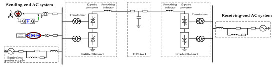
Figure 1.
Structure of doubly fed induction generator (DFIG) wind farm connected with series compensated transmission network.
2.1. Model of DFIG
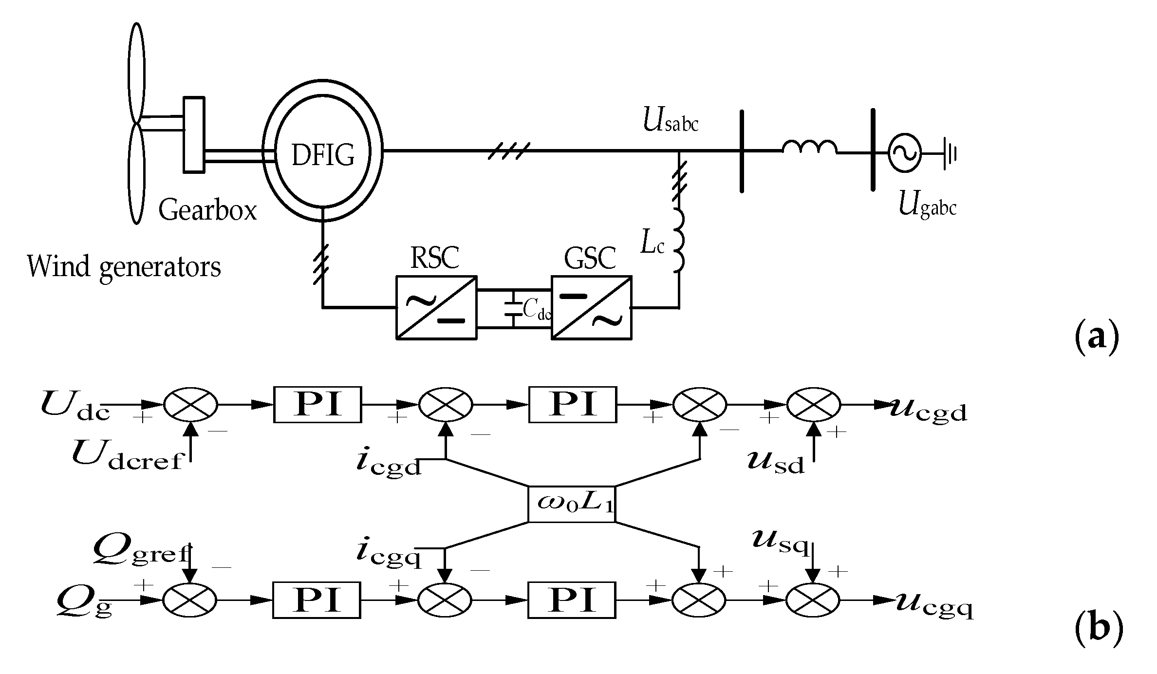
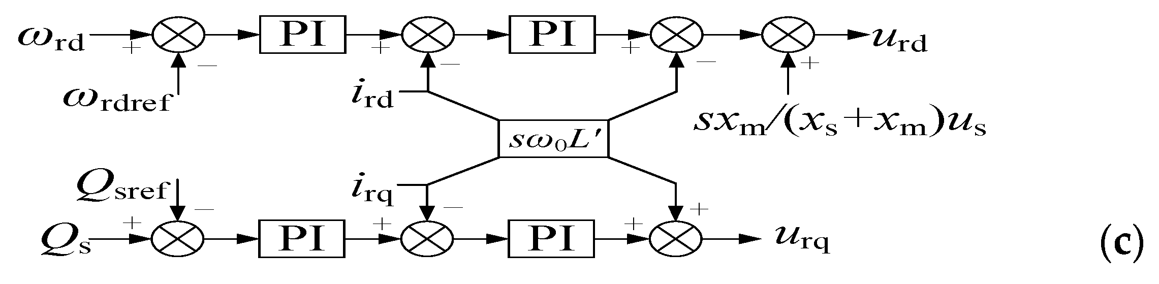
The DFIG topology structure and its control strategy are shown in Figure 2, consisting of wind turbines, an induction generator, a rotor-side converter (RSC), and a grid-side converter (GSC). The definitions of variables in Figure 2 are shown in Table A1 (Appendix A). The stator is directly connected to the network, and the rotor is connected to the grid through the RSC and GSC. The RSC and GSC usually use voltage vector-oriented control [22,23]. In order to maximize the utilization of wind energy, the RSC adopts the maximum power point tracking (MPPT) control strategy, whereas the GSC takes DC voltage and reactive power as the control targets.
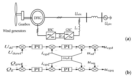
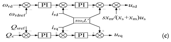
Figure 2.
The topology and control system of a DFIG: (a) topology structure; (b) control strategy of the grid-side converter (GSC); (c) control strategy of the rotor-side converter (RSC).
The mathematical model of the DFIG, as shown in [24], is linearized at the equilibrium point to obtain the linearized model shown in Equation (1).
where ADFIGs, BDFIGs, CDFIGs, and DDFIGs are the state matrix, input matrix, and output matrix of DFIGs; the state variables are ΔxDFIGs = [Δωr, Δψsd, Δψsq, Δψrd, Δψrq, Δigd, Δigq, Δudc, Δx1~Δx8], and ΔxDFIGs is a 16 × 1 matrix; the input and output variables are ΔuDFIGs = [Δusd, Δusq]T and ΔyDFIGs = [Δisd, Δisq]T, and ΔuDFIGs and ΔyDFIGs are 2 × 1 matrices. The transfer function of DFIGs is denoted in Equation (2).
2.2. Model of SG
The topological structure of an SG was described in [20], consisting of an electrical part and shafting part. The electrical part includes stator/rotor excitation and voltage, and the shafting part is equivalent to six mass blocks, namely, a high-pressure cylinder (HP), intermediate-pressure cylinder (IP), low-pressure cylinder A (LPA), low-pressure cylinder B (LPB), generator, and exciter. There are five natural oscillation frequencies in the shaft system, which are 15.71 Hz (torsional mode 1, TM1), 20.21 Hz (TM2), 25.55 Hz (TM3), 32.28 Hz (TM4), and 47.46 Hz (TM5), respectively, of which TM5 is not considered in this paper.
The mathematical model of an SG was shown in [20], linearized at the equilibrium point, and the linearized mode of the SG was obtained, as represented by Equation (3).
where ASG, BSG, CSG, and DSG are the state matrix, input matrix, and output matrix of SG; the state variables are ΔxSG = [Δω1~Δω6, Δδ1~Δδ6, ΔT1~ΔT3, Δα, Δμ, Δif, ΔiD, Δig, ΔiQ, ΔEfd], and ΔxSG is a 22 × 1 matrix; the input and output variables are ΔuSG = [Δud, Δuq]T and ΔySG = [Δid, Δiq]T, and ΔuSG and ΔySG are 2 × 1 matrices. The definitions of variables are shown in Table A2 (Appendix A).
The transfer function of SG is further obtained as shown in Equation (4).
2.3. Model of HVDC
The topology and mathematical model of HVDC were shown in [21]. The rectifier of HVDC adopts constant current control and the inverter-side controller adopts constant turn-off angle control. The linearized model structure can be given as
where AHVDC, BHVDC, CHVDC, and DHVDC are the state matrix, input matrix and output matrix of HVDC; the state variables are ΔxHVDC = [ΔIrd, ΔIrq, ΔIdc1, ΔIdc2, ΔVdc, ΔVpccd, ΔVpccq, ΔVcr2d, ΔVcr2q, ΔILr1d, ΔILr1q, ΔVcr3d, ΔVcr3q, ΔVcr4d, ΔVcr4q, ΔILr2d, ΔILr2q, Δx9~Δx12], and ΔxHVDC is a 21 × 1 matrix; the input and output variables are ΔuHVDC = [ΔVrd, ΔVrq, ΔIdc]T and ΔyHVDC = [ΔIrd, ΔIrq]T, and ΔuHVDC is a 3 × 1 matrix and ΔyHVDC is a 2 × 1 matrix. The definitions of variables are shown in Table A3 (Appendix A).
The transfer function of HVDC can be obtained as shown in Equation (6):
3. Electromechanical Coupling Characteristics of Equipment
According to the SG linearized model, the electromagnetic torque disturbance ΔTe can be expressed as shown in Equation (7).
where ω0 is the SG rotor speed initial value, ωbase is the reference value of the SG, and ωbase = 60 Hz.
L1(s) and L2(s) represent the transfer function relationship between current and flux, and the expressions are denoted in Equation (8).
According to Equation (7), the SG electromagnetic torque disturbance is related to the rotor speed disturbance and voltage disturbance, and the voltage disturbance is correlated with the current disturbance and grid structure. The expression of voltage disturbance is considered as shown in Equation (9).
where Z11, Z12, Z21, and Z22 are the grid impedance matrix elements, and the current disturbance expression is shown in Equation (10).
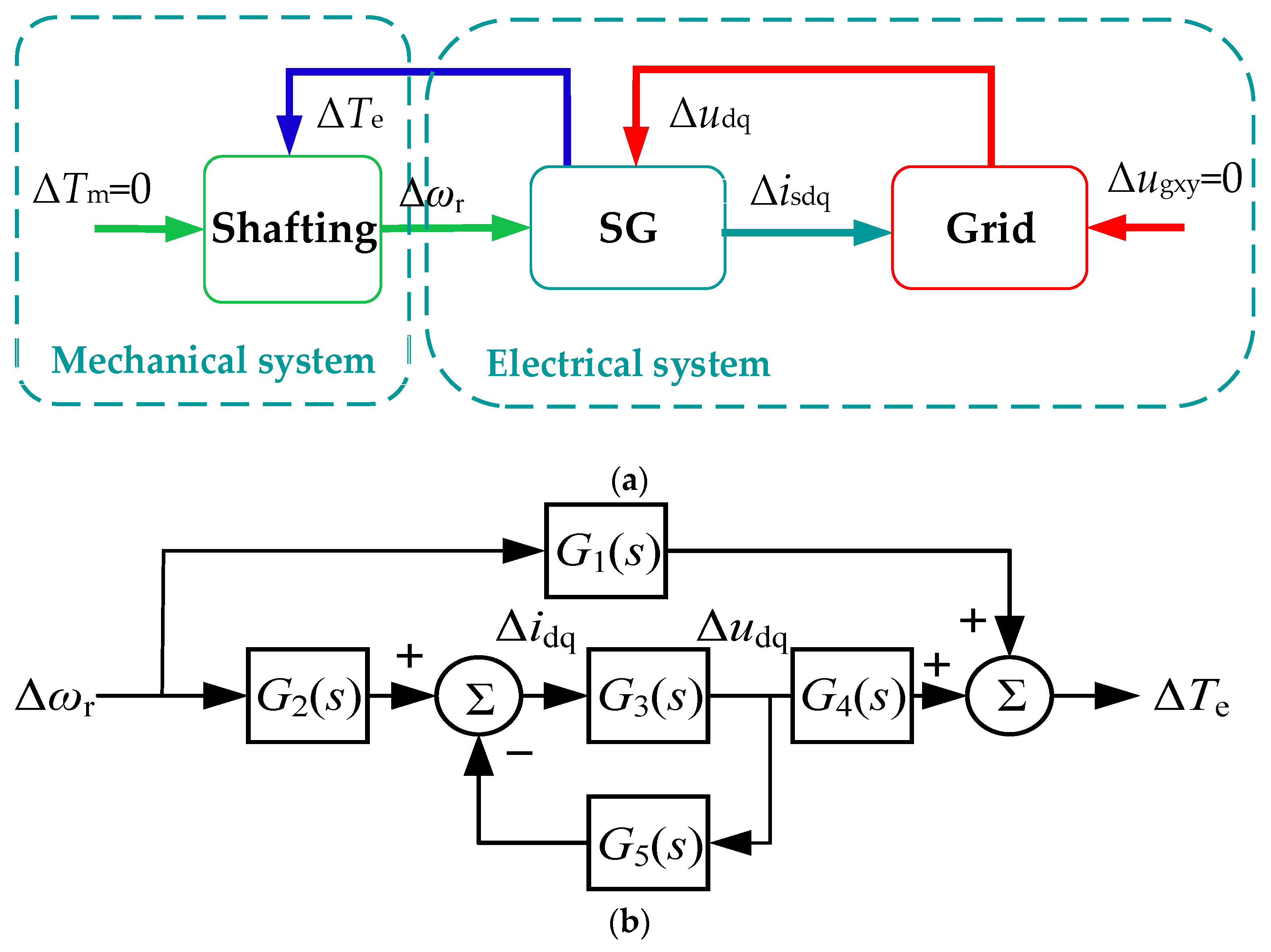
Equations (7)–(10) reflect the formation mechanism of SG electromagnetic torque, thus giving the formation mechanism diagram shown in Figure 3a. The SG speed disturbance is the input signal, and the electromagnetic torque is composed of two branches, of which the first branch is mainly determined by the SG electrical part and the second branch is codetermined by the SG electrical part and the grid. The expressions of G1(s), G2(s), G3(s), G4(s), and G5(s) in Figure 3b are shown in Equation (A1) (Appendix A).
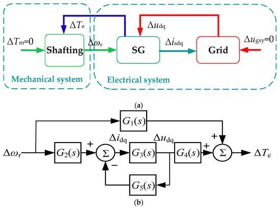
Figure 3.
The electromagnetic torque formation mechanism of a synchronous generator (SG): (a) SG electromechanical coupling mechanism; (b) speed disturbance transfer relationship.
It can be seen from Figure 3 that the SG speed disturbance transfer function can be obtained.
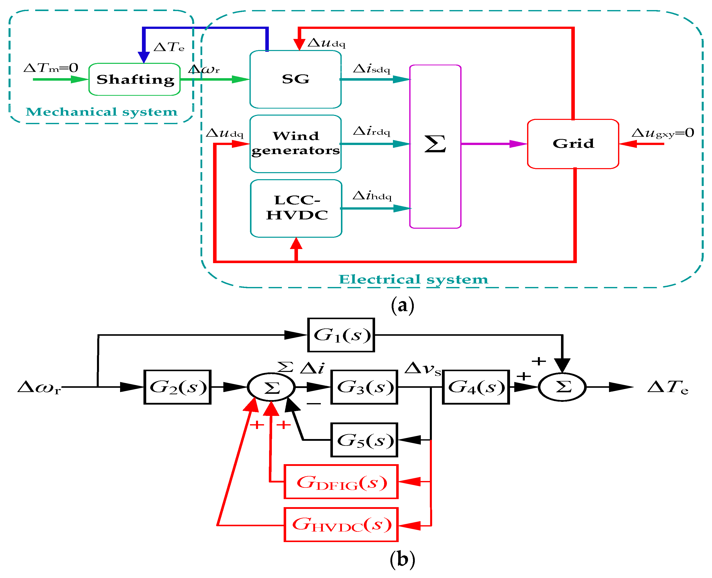
When the DFIG and HVDC are connected to the system, the mechanism of interaction with the SG is shown in Figure 4. It can be seen that the rotor disturbance Δωr of the SG is the input disturbance of the electrical system. The output current disturbance Δisdq is formed through the electromagnetic coupling relationship of the electrical part. On the one hand, Δisdq directly forms the electromagnetic torque disturbance ΔTe and acts on the rotor; on the other hand, the terminal voltage disturbance Δudq of the SG, wind turbines, and HVDC is formed by the grid coupling. The SG terminal voltage disturbance through its electromagnetic coupling relationship intensifies ΔTe and Δisdq; then, Δisdq interacts with the terminal voltage disturbances of wind turbines and HVDC to produce current disturbances Δirdq and Δihdq. Furthermore, Δirdq and Δihdq are superimposed to continue the grid function and form a new terminal voltage disturbance Δudq, which further aggravates ΔTe until the system rebalances or loses stability.
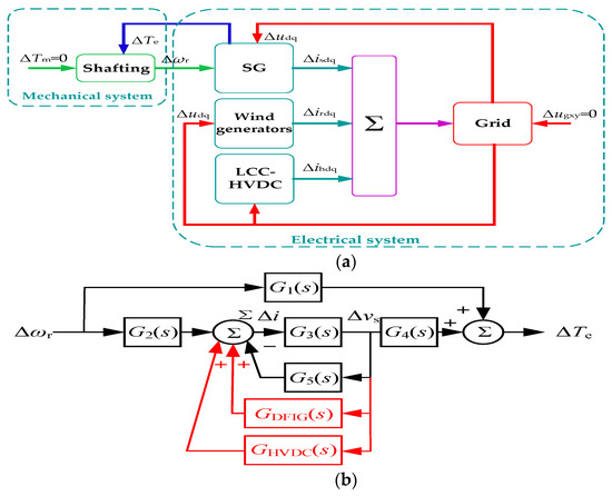
Figure 4.
The dynamic interaction between various equipment and the SG: (a) SG electromechanical coupling mechanism; (b) speed disturbance transfer relationship.
It can be seen from Figure 4 that the rotational speed disturbance transfer function among the DFIG, HVDC, and SG is considered as shown in Equation (12).
The above analysis reflects the influence of the electromechanical transient process of power electronic equipment on the electromechanical transient process of current magnetization equipment. The electromechanical coupling process among wind turbines, HVDC, and SGs is revealed from the mechanism. At present, eigenvalue analysis, complex torque analysis, impedance analysis, and the time-domain simulation method are commonly used to analyze system SSO problems. Among them, eigenvalue analysis can obtain the inherent mode of the system and judge the stability of the system at one operating point, but it cannot explain the subsynchronous interaction mechanism clearly. Whether the complex torque analysis is applicable to multimachines and multi-power electronics systems is still inconclusive, and impedance analysis can only determine the stability of the subsystem but not the entire system. The above methods are difficult to ensure calculation accuracy when studying the SSO problem of complex systems including DFIGs, SGs, and HVDC, while the time-domain simulation method can guarantee model integrity and calculation accuracy to the maximum extent. Therefore, this paper studies the influence of various equipment on SG shafting using the identification signal injection method.
4. Influence of Various Online Equipment on the Damping Characteristics of SGs
4.1. Additional Excitation Signal Injection Method
Common SG identification methods include the stator-side additional current injection method and rotor-side additional excitation signal injection method. The latter is used in this paper. The advantages of this method are that the frequency, amplitude, and time length of the excitation signal can be changed according to needs, and all concerned modal attenuation coefficients can be identified; in online application, due to the controllable amplitude, it can ensure the safety of the shafting system without affecting the normal operation of the system. From the dynamic coupling mechanism of various equipment, the torsional vibration of the SG shafting system is caused by the transmission of wind turbines via HVDC, which is manifested in the rotor speed oscillation; that is, the speed contains abundant electromechanical coupling information. If a controllable disturbance is applied to stimulate the rotation speed oscillation and to observe the response characteristics of the rotation speed after the disturbance is removed, the electromechanical coupling characteristics among the wind turbines, HVDC, and SGs can be judged, and then the contribution of each equipment to the shaft torsional vibration of the unit can be identified.
Taking the rotor motion equation as an example, the variation rules of rotor angle and its frequency are as follows when there is external disturbance:
where the electromagnetic torque ΔTek = −Acos(ωst).
Assuming the angle increment Δδk(t = 0) = 0, the torsional vibration of SG can be expressed as
where Δδk,t(t) is the transient response that only exists for a period of time, and Δδk,s(t) is the forced response under the excitation of the injected signal. It can be seen that the SG rotor dynamic process contains attenuation components and forced excitation, and the attenuation coefficient can characterize the modal damping of the system.
When the excitation signal is removed, the rotational speed of the torsional vibration mode decays exponentially. Solving Equation (16) can obtain the expression of shafting torsional vibration, which can be expressed as shown in Equations (17) and (18).
where Cθ, Cω are coefficients, and t0 is the time to remove the excitation. It can be seen from Equation (18) that, after the excitation is withdrawn, the modal speed changes in the form of attenuated oscillation, and the attenuation rate is the sum of mechanical damping and electrical damping. The total mode can be obtained by identifying the attenuation rate of the torsional vibration mode speed after removing the excitation.
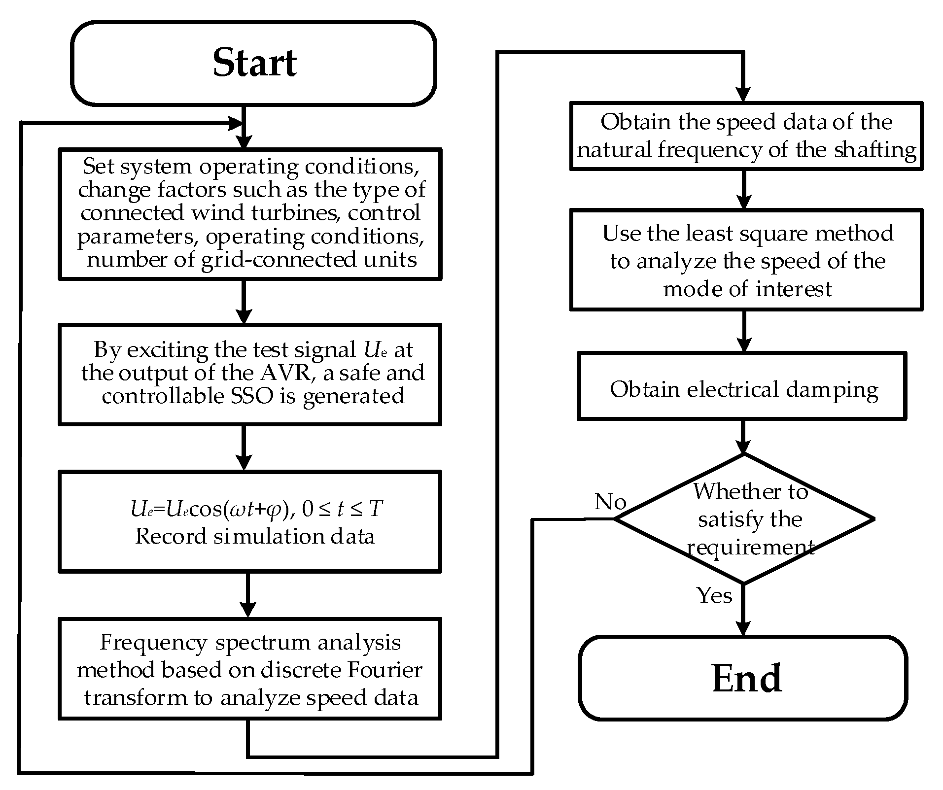
The basic principle of the additional excitation signal injection method is shown in Figure 5 [25], which shows that the modal signal generator superimposes the excitation test signal us with controllable angular velocity, amplitude, and duration to the output of automatic voltage regulator (AVR). The us can generate the electromagnetic torque disturbance ΔTe, and it excites a safe and controllable SSO in shafting system. After removing us, the change in generator speed depends on the result of the interaction between the mechanical damping and electrical damping of the system, and the damping can be identified using the spectrum analysis method on the basis of discrete Fourier transform. Since the influence of mechanical damping is not considered in this paper, the mechanical damping was set as 0. The main process of the injection method is depicted in Figure 6.
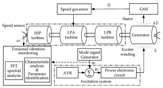
Figure 5.
Basic principle of excitation-signal-injection method.
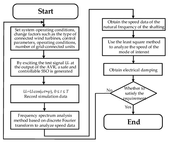
Figure 6.
Flowchart of the proposed identification approach.
4.2. Influence of Access to Various Equipment on SG Damping Characteristics
In order to illustrate the feasibility of the above method, the system shown in Figure 1 was taken as an example. The transmission capacity of HVDC was 800 MW, and the output power of the SG was 600 MW. The installed capacity of a single DFIG was 1.5 MW, and the grid-connected number and wind speed of DFIG were 1500 and 4 m/s.
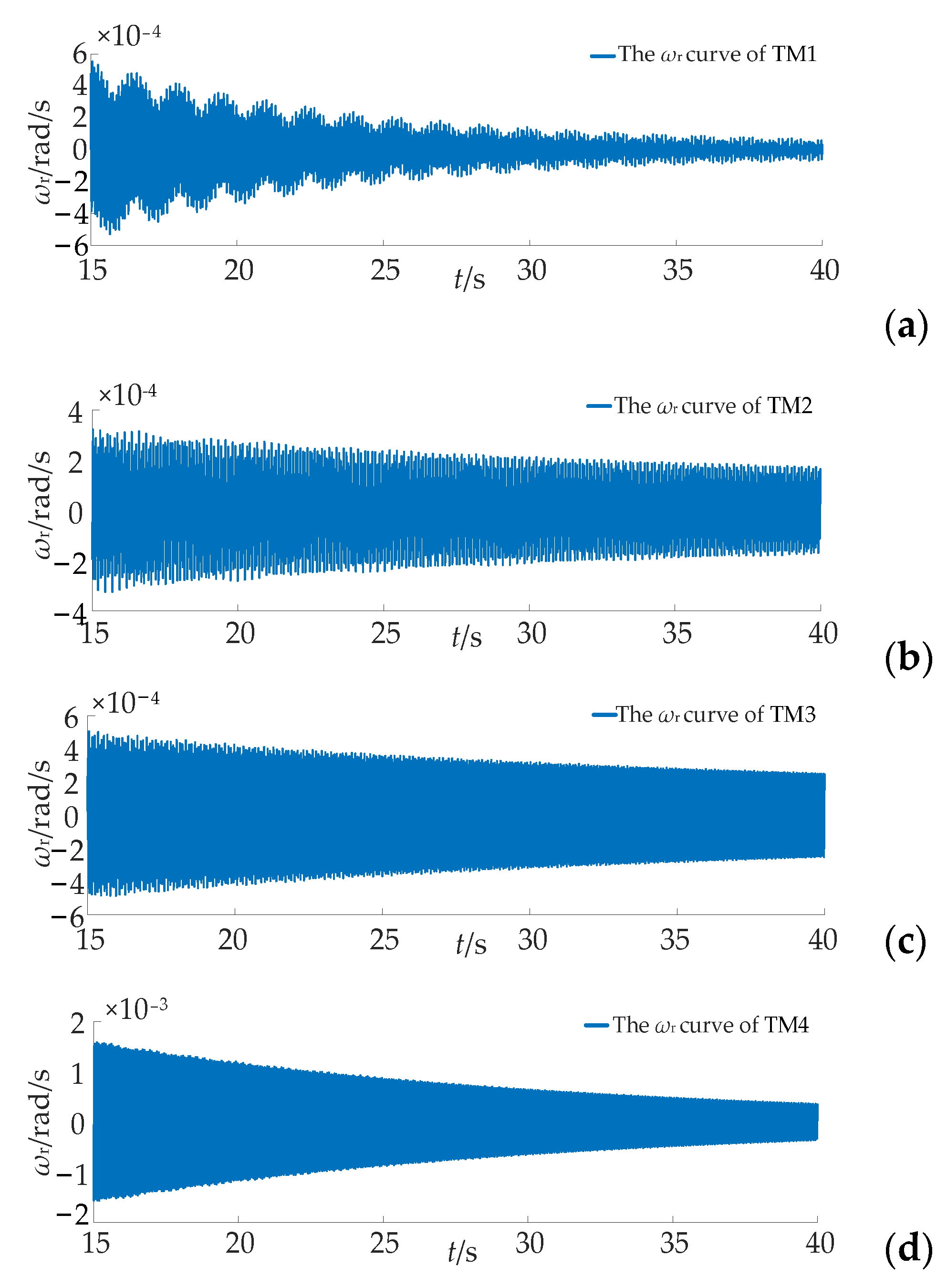
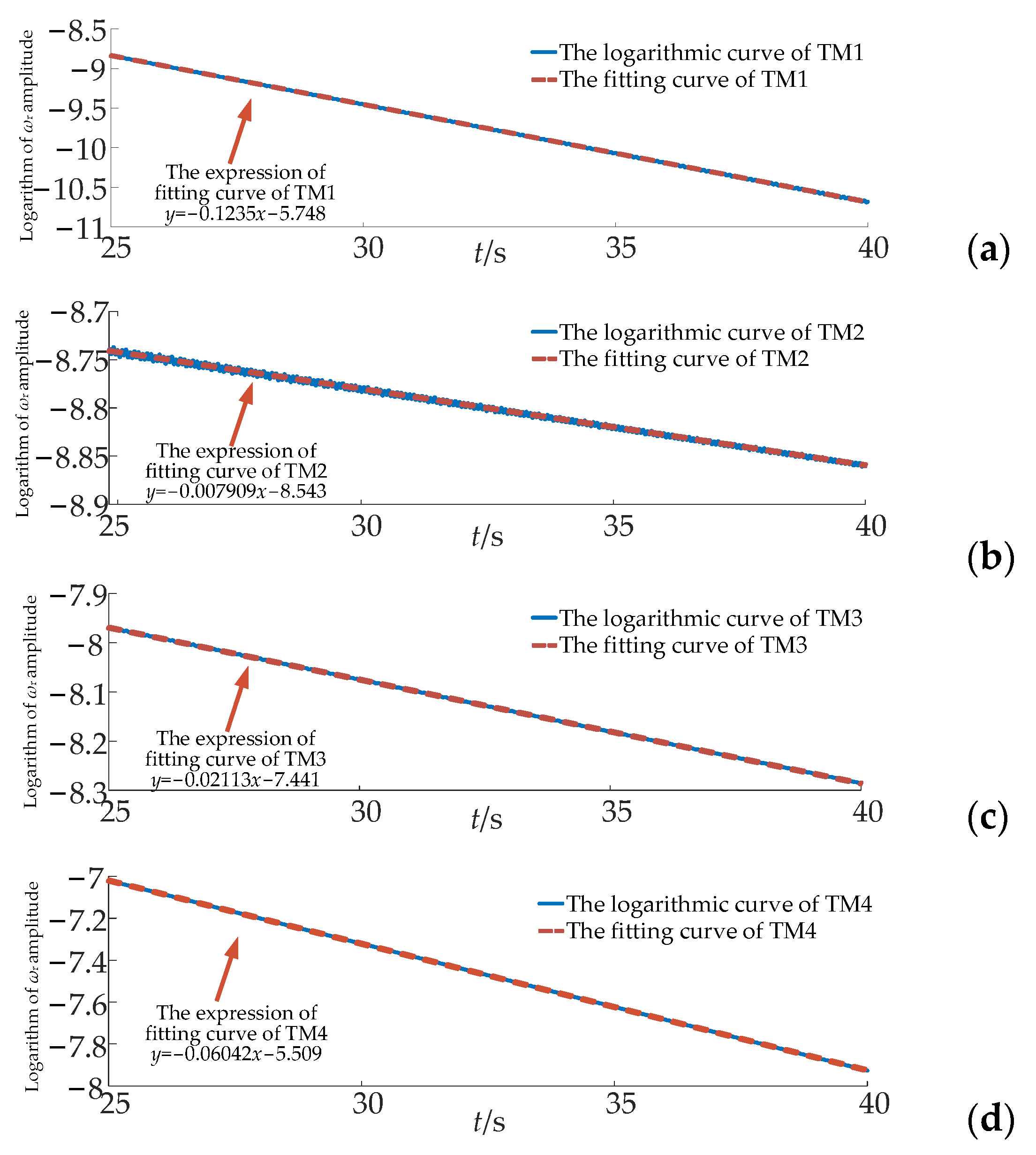
When t = 0 s, the excitation signal disturbance was added, and then the signal was removed at 15 s. The rotational speed curve of SG shafting in torsional vibration mode is shown in Figure 7. The logarithm of the ωr amplitude was taken and curve-fitting was performed. The fitting results are shown in Figure 8, and the attenuation coefficients of TM1–TM4 were −0.1235, −0.007909, −0.02113, and −0.06042, respectively.
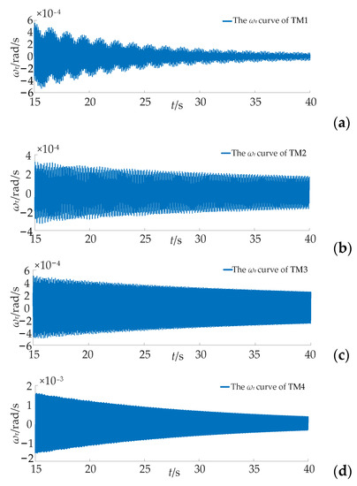
Figure 7.
The rotor speed curve of SG torsional mode after repealing the disturbance: (a) TM1; (b) TM2; (c) TM3; (d) TM4.
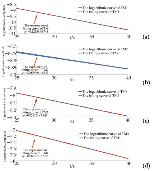
Figure 8.
The comparison diagram of the change curves of the amplitude of ωr after taking the logarithm and fitting curves: (a) TM1; (b) TM2; (c) TM3; (d) TM4.
In order to further analyze the influence of wind speed and control parameters on the torsional vibration of the SG shafting system under the condition of fixed HVDC transmission capacity, the evolution law of the influence of various factors on the torsional vibration was studied by taking a single-DFIG model and a two-machine parallel model as examples.
4.2.1. Influence of Access to Single Equivalent DFIG on SG Shafting
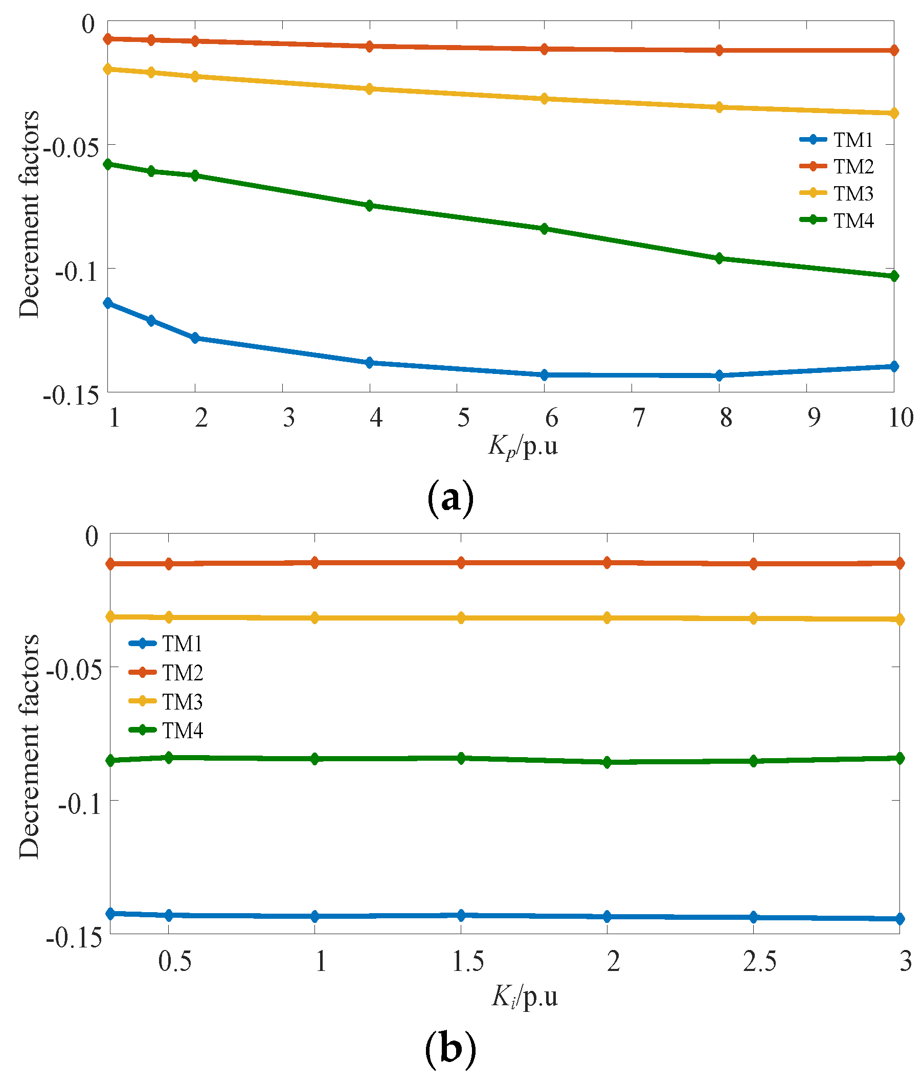
The wind speed was 4 m/s, the transmission capacity of HVDC was 800 MW, the output power of the SG was 600 MW, and the installed capacity of a single DFIG was 1.5 MW. When 1500 units were connected in parallel, the attenuation coefficient of each SG torsional vibration mode was as shown in Figure 9 under the control parameters of different DFIG rotor converter current inner loops.
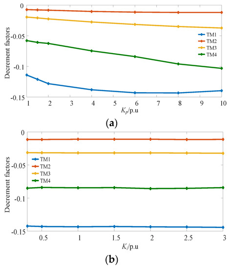
Figure 9.
Damping coefficient for each torsional mode of SG under different rotor converter current inner loops: (a) different Kp; (b) different integral coefficient of the current inner loop (Ki).
It can be seen from Figure 9 that, when the number of grid-connected DFIGs was given, and when Kp changed from 1 p.u. to 10 p.u., the attenuation coefficients of the torsional vibration modes of SG shafting generally showed a trend of decrease, whereby the attenuation coefficient of TM1 decreased 1.2-fold, the attenuation coefficients of TM2 and TM3 decreased 1.7-fold and 1.9-fold, and the attenuation coefficient of TM4 decreased 1.8-fold. The damping characteristics of the modes were enhanced, and, within the same time range, TM1 changed more obviously. As the integral coefficient of the current inner loop increased, the attenuation coefficients of the torsional modes of the SG did not change significantly.
The installed capacity of a single DFIG was 1.5 MW, the output power of the SG was 600 MW, and the output power of HVDC remained at 800 MW. Under different operating conditions of grid-connected DFIGs, the attenuation coefficients of the torsional mode of the SG were as shown in Figure 10.
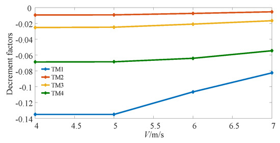
Figure 10.
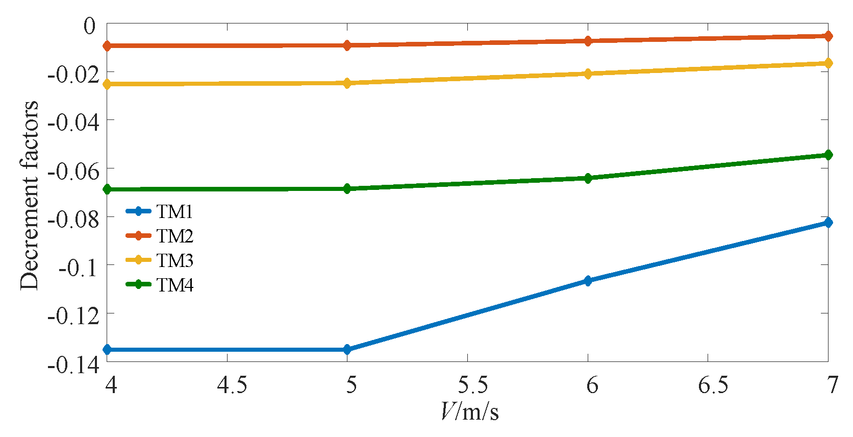
Damping coefficient for each torsional mode of SG under different operating conditions.
It can be seen from Figure 10 that, as the wind speed increased from 4 m/s to 7 m/s, the attenuation coefficients of the torsional modes of SG shafts increases, and the mode damping characteristics weakened. Specifically, the attenuation coefficients of TM1–TM4 increased 1.6-fold, 1.8-fold, 1.5-fold, and 1.3-fold, respectively.
From all the above results, it can be seen that the Ki of DFIGs, as well as the operating conditions of the wind turbines, can affect the damping characteristics of the SG, while the setting of Ki has little effect on the SG damping characteristic.
4.2.2. Influence of Parallel Connection of Two DFIGs on SG Shafting
Considering that the actual wind turbines are often distributed in different regions, the wind speed and the number of grid-connected units in different regions may be quite different. Therefore, this section takes two DFIGs in parallel as an example, considering the geographical distribution of wind turbines; furthermore, it studies the influence of the control parameters and the change in operating conditions on SG shafting in a wind–thermal bundled system transmitted via HVDC.
When the operating condition of DFIGs was 4 m/s, the number of grid-connected units was 1500, and the output power of HVDC and SG was 800 MW and 600 MW, respectively, the Kp of the two DFIGs increased from 1 p.u to 10 p.u. The attenuation coefficient of TM1 of the SG shafting system is shown in Table 1, and the other modes are shown in Table A4, Table A5 and Table A6 (Appendix B); in the same way, the current inner loop control integral coefficients of the two DFIGs increased from 0.5 p.u to 3 p.u. The attenuation coefficient of TM1 is shown in Table 2. Table 1 and Table 2 show that (1) when the Kp of group1 was constant, with the increase in Kp of the current inner loop of group2, the damping characteristics of the system were enhanced and the oscillation frequency decreased, (2) when the Ki of group1 was constant, with the increase in Ki of group2, the damping characteristics of the SG shafting system changed little, and (3) in the two-DFIG parallel system, the increase in proportional coefficient of the DFIG inner loop was conducive to the stability of TM1, and the change trend was basically the same as the conclusion of the single system.

Table 1.
Damping coefficient for TM1 of SG under different Kp.
Table 2.
Damping coefficient for TM1 of SG under different Ki.
When Kp was 3 p.u, the capacity of HVDC was 800 MW, and the SG output power was 600 MW, the operating condition of the DFIGs increased from 4 m/s to 7 m/s, and the attenuation coefficient of SG shafting torsional (TM1) was as shown in Table 3. It can be seen from Table 3 that with the increase in wind speed of Group 2, the damping characteristics of the system weakened and the oscillation frequency increased as the wind speed of group1 was constant. Therefore, in the two-machine parallel system, the increase in DFIG operating conditions was harmful to the stability of TM1, and the change trend was consistent with the conclusion of the single system.
Table 3.
Damping coefficient for TM1 of SG under different operating conditions.
4.2.3. Influence of SG Parameters on SG Shafting
The influence of SG parameters on the torsional vibration of SG shafting were not considered in the above analysis. This section mainly analyzes the influence of AVR and mechanical damping coefficient of SG on the torsional modes of each shafting. The AC exciter adopts the IEEE AC exciter module AC1A, and the transfer function block diagram is shown in Figure A1 (Appendix C).
When the wind speed of the DFIGs was 4 m/s, the number of grid-connected units was 1500, the HVDC transmission power was 800 MW, and the output power of the SG was 600 MW, under different AVR control parameters (KA and TA), the attenuation coefficients of each torsional mode of SG were as shown in Table 4 and Table 5. The attenuation coefficients of each torsional mode of SG are shown in Table 6 under different mechanical damping coefficients (Dm).
Table 4.
Damping coefficient for TM1–TM4 of SG under different KA (TA = 0.02).
Table 5.
Damping coefficient for TM1–TM4 of SG under different TA (KA = 50).
Table 6.
Damping coefficient for TM1–TM4 of SG under different TA (KA = 50).
From Table 4, Table 5 and Table 6, it can be seen that the change in AVR control parameters had little influence on each torsional mode of the SG. The mechanical damping coefficient had a great influence on the torsional mode of the SG, whereby larger coefficients were more conducive to the stability of each torsional mode.
5. Time-Domain Simulation Verification
In order to verify the correctness of the theoretical analysis, a simulation model of DFIGs, SGs, and HVDC connected to a grid system was built in EMTDC/PSCAD. Among them, the SG adopted the IEEE SSR first standard model, and the simulation parameters of SG were as shown in [17]. The HVDC adopted the CIGRE Benchmark Model, whose rated transmission power was 1000 MW. The simulation parameters of HVDC and DFIG are shown in Table A10 and Table A11 (Appendix C).
5.1. Influence of Single Machine on Torsional Vibration of SG Shafting
5.1.1. Different Current Inner Loop Control Parameters
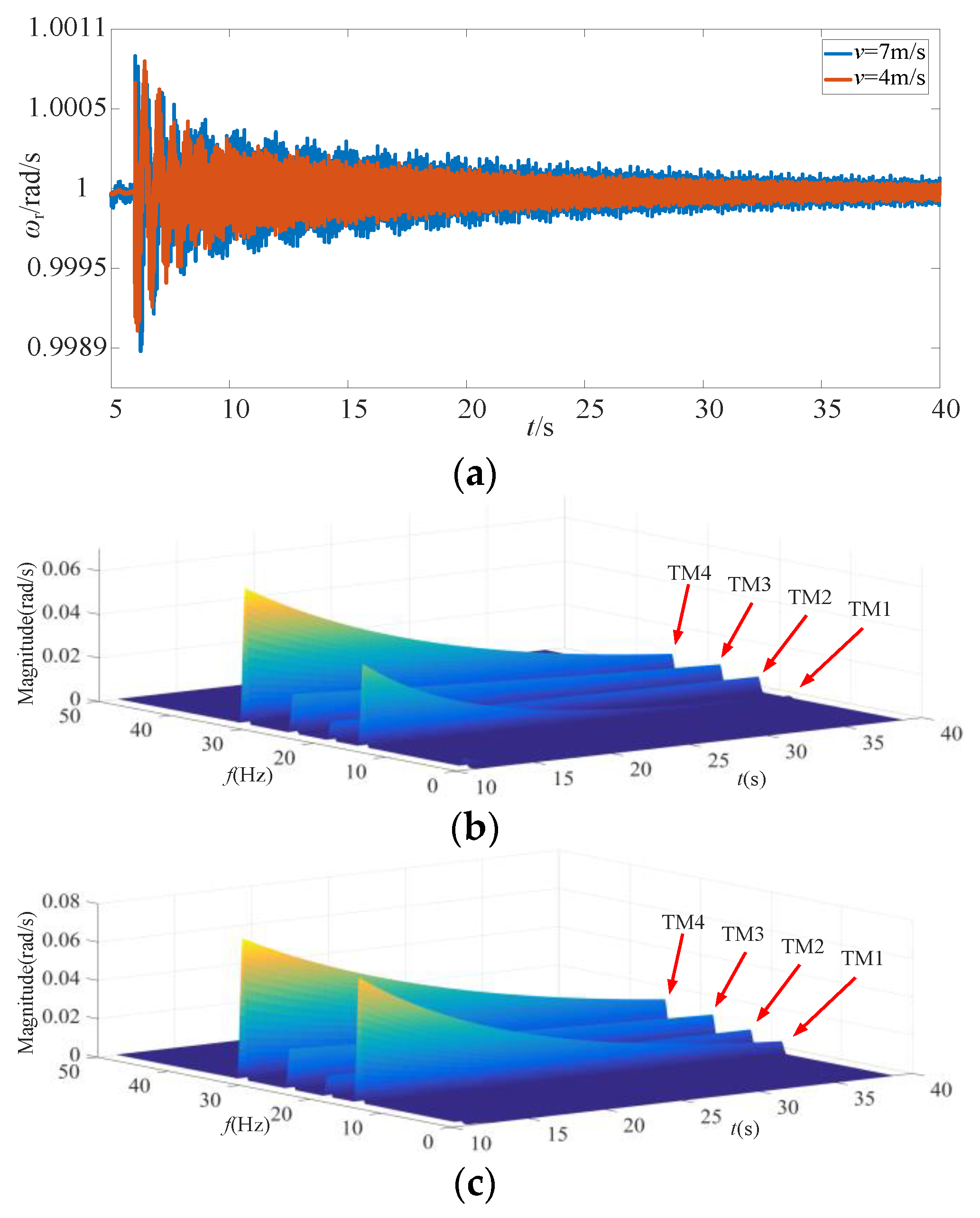
The wind speed of the DFIGs was 4 m/s, the number of grid-connected units was 1500, the HVDC transmission power was 800 MW, and the output power of the SG was 600 MW. A three-phase short circuit fault occurred in the system at t = 6 s, and the duration was 75 ms. The SG rotor speed response curve under the Kp of DFIGs is shown in Figure 11a. Time–frequency analysis was used to analyze the rotor speed data, and the time–frequency analysis results are shown in Figure 11b,c.
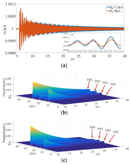
Figure 11.
Rotor speed response of SG and the time–frequency analysis result: (a) rotor speed response curve; (b) Kp = 1.5 p.u; (c) Kp = 8 p.u.
As can be seen from Figure 11, with the increase in Kp, the attenuation trend of TM1 changed most significantly compared with other modes, and the mode damping was enhanced. The time-domain simulation results were consistent with the analysis results in Section 4.2.1.
5.1.2. Different Operation Conditions
When the control parameters of the DFIGs were constant, the number of grid-connected units was 1500, and the output powers of the HVDC and the SG were fixed, the system had a three-phase short circuit fault at t = 6 s with a duration of 75 ms. The results of the rotor speed response curve and time–frequency analysis under different operating conditions of DFIGs are shown in Figure 12.

Figure 12.
Rotor speed response of SG and the time–frequency analysis result: (a) rotor speed response curve; (b) v = 4 m/s; (c) v = 7 m/s.
Comparing Figure 12b with Figure 12c, it can be concluded that, when the wind speed of DFIGs increased from 4 m/s to 7 m/s, the change trend of TM1 was more obvious than the other three modes and TM1 damping became weaker, which was not conducive to system stability. The change trend was consistent with the identification results in Figure 10.
5.2. Influence of Two-Machine Parallel System on Torsional Vibration of SG Shafting
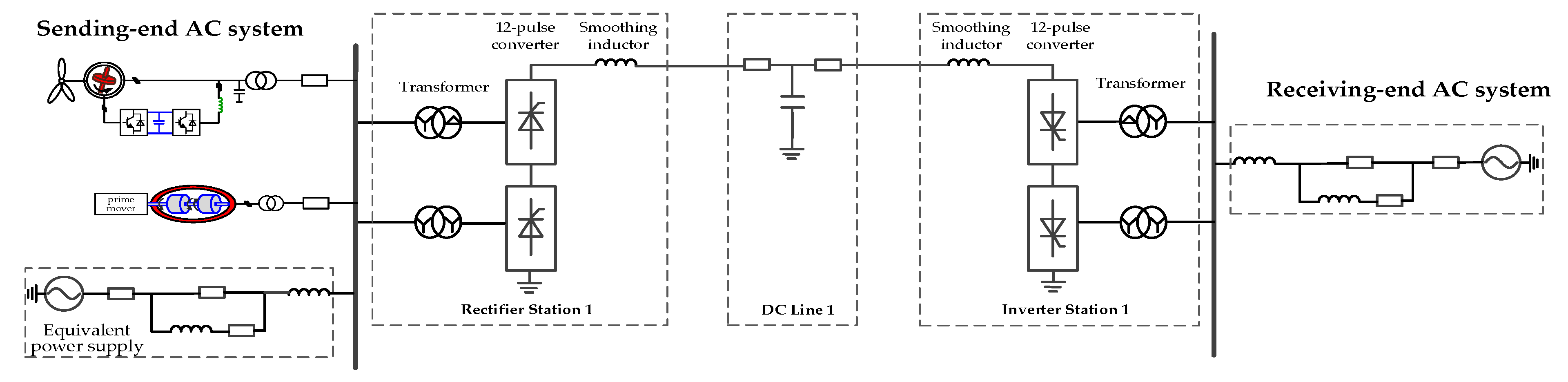
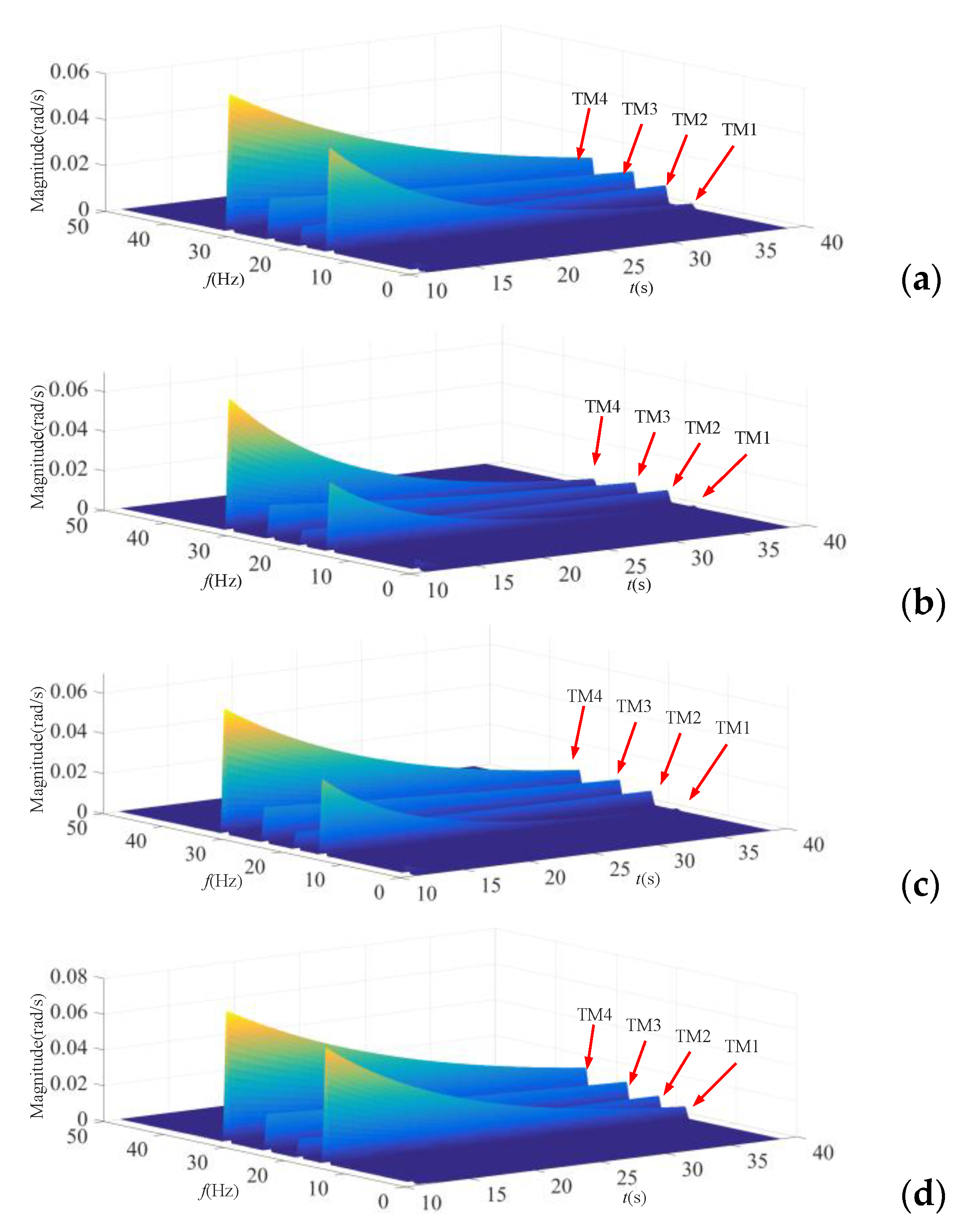
The system parameters were the same as in Section 5.1. In this section, the two-machine parallel system was simulated and verified. The torsional vibration of the SG transmitted via an HVDC system was analyzed, accounting for the regional differences in wind turbines, caused by different current inner loop control parameters, operating conditions, and the number of grid-connected units. The results of the SG rotor speed response curve and the time–frequency analysis are shown in Figure 13 and Figure 14.
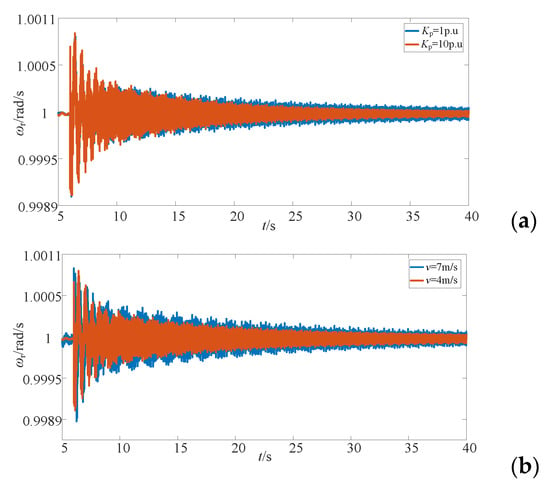
Figure 13.
Rotor speed response of SG: (a) Kp = 1 p.u–10 p.u; (b) v = 7 m/s–4 m/s.

Figure 14.
Rotor speed response of SG and the time–frequency analysis result: (a) Kp = 1 p.u; (b) Kp = 10 p.u; (c) v = 4 m/s; (d) v = 7 m/s.
From the time-domain analysis, it can be seen that, when the Kp of the RSC in the DFIG increased and the operating conditions decreased, it was conducive to the stability of the system.
6. Conclusions
This paper proposed a torsional vibration analysis method for a system containing HVDC, DFIGs, and SGs, using the additional excitation signal injection method. It revealed the torsional modes of the SG shafting caused by DFIGs connected to the grid. The main conclusions are as follows:
(1) In a typical wind–thermal bundled system transmitted via HVDC, the electromagnetic transient process among wind turbines, SGs, and HVDC influences the electromechanical transient process of the system. There are some factors, such as the types of grid-connected wind turbines, main control parameters, operating conditions, and; the transmission power and control parameters of HVDC that affect the torsional modes of the SG to some extent.
(2) For the DFIG and SG system transmitted via HVDC, under the given HVDC transmission capacity, as the current inner loop control parameters of the RSC of the DFIG decreased (Kp = 10 p.u–1 p.u), the damping characteristics of each torsional mode of the SG decreased; as the operating conditions of the DFIG decreased (v = 7–4 m/s), the damping characteristics of each torsional mode gradually increased. With the increase in mechanical damping coefficient (Dm = 0.05 p.u–2 p.u), the damping of each torsional mode increased, which was beneficial to the stability of the system.
Author Contributions
Conceptualization, Q.J. and G.Y.; methodology, Q.J.; software, J.W.; validation, J.W. and K.L.; formal analysis, D.W.; investigation, J.W. and K.L.; resources, Q.J.; data curation, J.W.; writing—original draft preparation, J.W.; writing—review and editing, J.W.; visualization, Q.J.; supervision, G.Y.; project administration, G.Y.; funding acquisition, G.Y. All authors have read and agreed to the published version of the manuscript.
Funding
This research was funded by the Joint Fund of the National Natural Science Foundation of China, grant number U1866601.
Conflicts of Interest
The authors declare no conflict of interest.
Appendix A
Table A1.
The definitions of variables for the DFIG.
Table A1.
The definitions of variables for the DFIG.
| Variable | Notation |
|---|---|
| Reactive power of stator | Qs |
| Active power of stator | Ps |
| Reactive power of grid | Qg |
| Voltage of rotor | ur |
| Current of rotor | ir |
| Voltage of grid | ug |
| Current of grid | ig |
| Voltage of stator | us |
| DC capacitor voltage | udc |
| Direct current capacitor | Cdc |
| Connection reactance | Lc |
| Output phase of phase-locked loop | θPLL |
| Wind speed | v |
| Rotor speed | ωr |
| The flux linkage of stator | ψs |
| The flux linkage of rotor | ψr |
| Output voltage of GSC | ucg |
| Output current of GSC | icg |
| Inductance of GSC | L1 |
| Inductance of rotor | L’ |
| Rated angular speed of the stator | ω0 |
| Slip | s |
| Mutual reactance | xm |
| Reactance of the stator | xs |
| State variables in the control system | x1~x8 |
Table A2.
The definitions of variables for the SG.
Table A2.
The definitions of variables for the SG.
| Variable | Notation |
|---|---|
| Stator voltage | Udq |
| Stator current | idq |
| Stator linkage | ψdq |
| Current of excitation winding | if |
| Current of damping winding in the d-axis | iD |
| Current of damping winding in the g-axis | ig |
| Current of damping winding in the Q-axis | iQ |
| Voltage of exciter | Efd |
| Location of speed relay | α |
| Opening angle of valve | μ |
| Motive power of steam turbine | T1~T3 |
| Rotational speed of 6-mass | ω1~ω6 |
| Rotor phase of 6-mass | δ1~δ6 |
Table A3.
The definitions of variables for HVDC.
Table A3.
The definitions of variables for HVDC.
| Variable | Notation |
|---|---|
| AC system voltage | Vr |
| AC system current | Ir |
| DC line current | Idc |
| DC line capacitance voltage | Vdc |
| AC bus voltage | VPCC |
| Filter capacitance voltage | Vcr |
| Filter capacitance current | ILr |
| State variables in the phase-locked loop controller | x9~x10 |
| State variables in the current loop controller | x11~x12 |
Appendix B
Table A4.
Damping coefficient for TM2 of SG under different Kp.
Table A4.
Damping coefficient for TM2 of SG under different Kp.
| Group 1 | 0.01 | 0.03 | 0.06 | 0.10 | |
|---|---|---|---|---|---|
| Group 2 | |||||
| 0.01 | −0.007161 | −0.008144 | −0.008696 | −0.008758 | |
| 0.03 | −0.008144 | −0.009209 | −0.01047 | −0.00998 | |
| 0.06 | −0.008696 | −0.01047 | −0.01127 | −0.01153 | |
| 0.10 | −0.008758 | −0.00998 | −0.01153 | −0.01187 | |
Table A5.
Damping coefficient for TM3 of SG under different Kp.
Table A5.
Damping coefficient for TM3 of SG under different Kp.
| Group 1 | 0.01 | 0.03 | 0.06 | 0.10 | |
|---|---|---|---|---|---|
| Group 2 | |||||
| 0.01 | −0.01933 | −0.02213 | −0.02481 | −0.0267 | |
| 0.03 | −0.02213 | −0.02492 | −0.02751 | −0.03029 | |
| 0.06 | −0.02481 | −0.02751 | −0.03117 | −0.03423 | |
| 0.10 | −0.0267 | −0.03029 | −0.03423 | −0.03682 | |
Table A6.
Damping coefficient for TM4 of SG under different Kp.
Table A6.
Damping coefficient for TM4 of SG under different Kp.
| Group 1 | 0.01 | 0.03 | 0.06 | 0.10 | |
|---|---|---|---|---|---|
| Group 2 | |||||
| 0.01 | −0.05832 | −0.06379 | −0.06968 | −0.07934 | |
| 0.03 | −0.06379 | −0.06961 | −0.07486 | −0.0854 | |
| 0.06 | −0.06968 | −0.07486 | −0.08635 | −0.09565 | |
| 0.10 | −0.07934 | −0.0854 | −0.09565 | −0.1061 | |
Table A7.
Damping coefficient for TM2 of SG under different operating conditions.
Table A7.
Damping coefficient for TM2 of SG under different operating conditions.
| Group 1 | 4 m/s | 5 m/s | 6 m/s | 7 m/s | |
|---|---|---|---|---|---|
| Group 2 | |||||
| 4 m/s | −0.009209 | −0.009532 | −0.008106 | −0.007434 | |
| 5 m/s | −0.009532 | −0.009037 | −0.007951 | −0.007308 | |
| 6 m/s | −0.008106 | −0.007951 | −0.007347 | −0.006515 | |
| 7 m/s | −0.007434 | −0.007308 | −0.006515 | −0.006187 | |
Table A8.
Damping coefficient for TM3 of SG under different operating conditions.
Table A8.
Damping coefficient for TM3 of SG under different operating conditions.
| Group 1 | 4 m/s | 5 m/s | 6 m/s | 7 m/s | |
|---|---|---|---|---|---|
| Group 2 | |||||
| 4 m/s | −0.02492 | −0.02601 | −0.02296 | −0.02096 | |
| 5 m/s | −0.02601 | −0.02437 | −0.02296 | −0.02103 | |
| 6 m/s | −0.02296 | −0.02296 | −0.02112 | −0.01892 | |
| 7 m/s | −0.02096 | −0.02103 | −0.01892 | −0.0183 | |
Table A9.
Damping coefficient for TM4 of SG under different operating conditions.
Table A9.
Damping coefficient for TM4 of SG under different operating conditions.
| Group 1 | 4 m/s | 5 m/s | 6 m/s | 7 m/s | |
|---|---|---|---|---|---|
| Group 2 | |||||
| 4 m/s | −0.06961 | −0.06708 | −0.0659 | −0.06452 | |
| 5 m/s | −0.06708 | −0.06817 | −0.0668 | −0.06279 | |
| 6 m/s | −0.0659 | −0.0668 | −0.06526 | −0.06163 | |
| 7 m/s | −0.06452 | −0.06279 | −0.06163 | −0.05618 | |
Appendix C
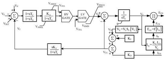
Figure A1.
The transfer function of AC1A.
Figure A1.
The transfer function of AC1A.
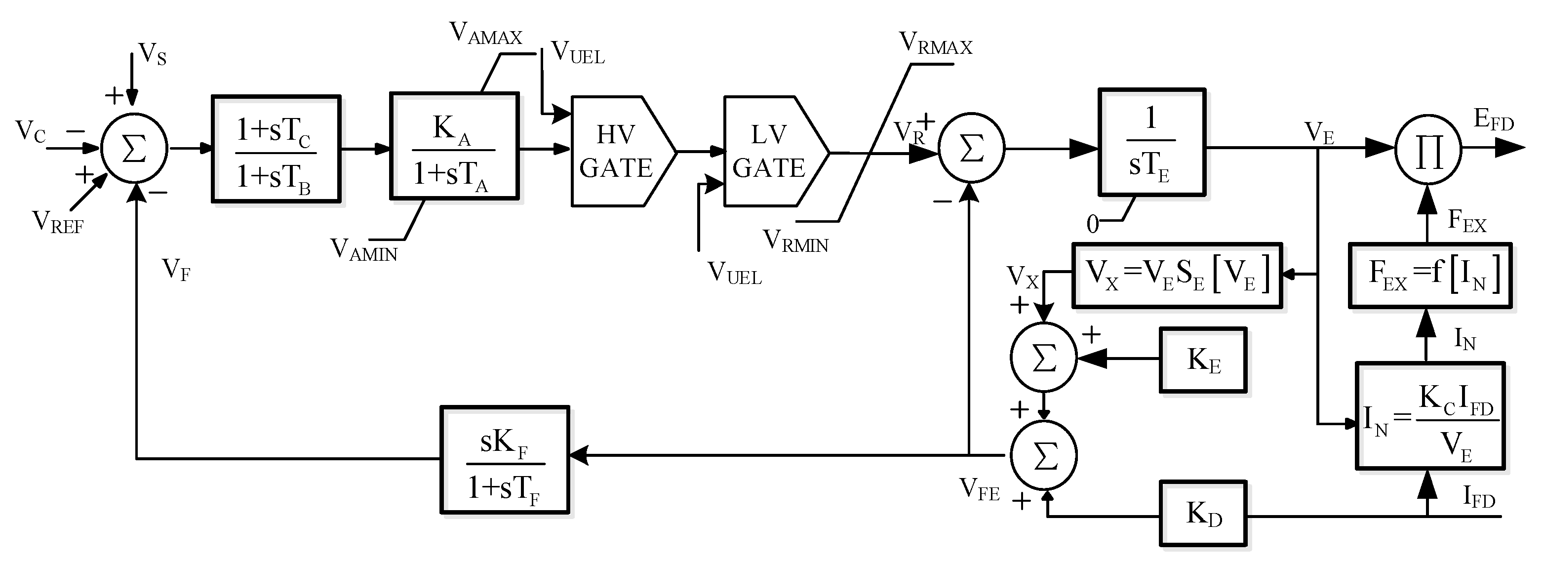
Table A10.
Main parameters of the DFIG.
Table A10.
Main parameters of the DFIG.
| Parameter | Unit/p.u. |
|---|---|
| Nominal capacity of DFIG PDFIG | 1.5 |
| Voltage of grid ug | 0.69 |
| Resistance of the stator rs | 0.0164 |
| Reactance of the stator xs | 0.255 |
| Resistance of the rotor rr | 0.0183 |
| Reactance of the rotor xr | 0.222 |
| Mutual reactance xm | 13.68 |
| DC capacitor voltage udc | 1.5 |
| Direct current capacity Cdc | 0.09 |
| Inductance of rotor L’ | 0.005 |
| Inductance of GSC L1 | 0.005 |
Table A11.
Parameters of the HVDC controller.
Table A11.
Parameters of the HVDC controller.
| Parameter | Unit/p.u. |
|---|---|
| Proportional coefficient of constant current controller KPr | 1.0989 |
| Integral coefficient of constant current controller Kir | 1/0.01092 |
| Proportional coefficient of turn-off angle controller KPi | 0.7506 |
| Integral coefficient of fixed turnoff angle controller Kii | 1/0.0544 |
| Proportional coefficient of measuring link Kmr | 0.5 |
| Integral coefficient of measuring link Tmr | 0.0012 |
| proportional coefficient of PLL KpPLL | 10 |
| Integral coefficient of PLL KiPLL | 50 |
| Proportional coefficient of constant current controller KPr | 1.0989 |
| Integral coefficient of constant current controller Kir | 1/0.01092 |
| Proportional coefficient of turn-off angle controller KPi | 0.7506 |
References
- Joselin, H.G.M.; Iniyan, S.; Sreevalsan, E.; Rajapandian, S. A review of wind energy technologies. Renew. Sustain. Energy Rev. 2007, 11, 1117–1145. [Google Scholar] [CrossRef]
- Ackermann, T. Wind Power in Power System; Wiley: Chichester, UK, 2005; pp. 7–23. [Google Scholar]
- China National Energy Administration. Operation of Wind Farm in First Half of 2020. Available online: http://www.nea.gov.cn/2020-07/31/c_139254298.htm (accessed on 31 July 2020).
- Energy Research Institute National Development and Reform Commission. China 2050 High Renewable Energy Penetration Scenario and Roadmap Study; Energy Research Institute National Development and Reform Commission: Beijing, China, 2015. [Google Scholar]
- Shair, J.; Xie, X.; Wang, L.; Liu, W.; He, J.; Liu, H. Overview of emerging subsynchronous oscillations in practical wind power systems. Renew. Sustain. Energy Rev. 2019, 99, 159–168. [Google Scholar] [CrossRef]
- Xie, X.R.; Liu, H.K.; He, J.B.; Liu, H.; Liu, W. On new oscillation issues of power systems. Proc. CSEE 2018, 38, 2821–2828. [Google Scholar]
- Xie, X.R.; Wang, L.P.; He, J.B.; Liu, H.; Wang, C.; Zhan, Y. Analysis of subsynchronous resonance/oscillation types in power systems. Power Syst. Technol. 2017, 41, 1043–1049. [Google Scholar]
- Li, M.J.; Yu, Z.; Xu, T.; He, J.B.; Wang, C.; Xie, X.; Liu, C. Study of complex oscillation caused by renewable energy integration and its solution. Power Syst. Technol. 2017, 41, 1035–1042. [Google Scholar]
- Bahrman, M.; Larsen, E.V.; Piwko, R.J.; Patel, H.S. Experience with HVDC-turbine-generator torsional interaction at square butte. IEEE Trans. Power Appar. Syst. 1980, 99, 966–975. [Google Scholar] [CrossRef]
- Piwko, R.J.; Larsen, E.V. HVDC System Control for Damping of Subsynchronous Oscillations. IEEE Power Eng. Rev. 1982, 2, 58. [Google Scholar] [CrossRef]
- Zhou, C.C.; Xu, Z. Damping analysis of subsynchronous oscillation caused by HVDC. Proc. CSEE 2003. [Google Scholar] [CrossRef]
- Yu, H.Y.; Zhao, G.L.; Hu, Y.T.; Gao, B.F.; Zhang, X.W. Damping characteristics of sub-synchronous torsional interaction of DFIG-based wind farm connected to HVDC system. J. Eng. 2017, 13, 1934–1939. [Google Scholar] [CrossRef]
- Gao, B.F.; Liu, Y.; Song, R.H.; Zhang, R.X.; Shao, B.B.; Li, R.; Zhao, S.Q. Study on subsynchronous oscillation characteristics of DFIG-based wind farm inteagrated with LCC-HVDC system. Proc. CSEE 2020, 40, 3477–3489. [Google Scholar]
- Yang, L.; Xiao, X.N.; Pang, C.Z. Oscillation analysis of a DFIG-based wind farm interfaced with LCC-HVDC. Sci. China Technol. Sci. 2014, 57, 2453–2465. [Google Scholar] [CrossRef]
- Gao, B.F.; Liu, Y.; Li, Y.H.; Zhao, F.; Shao, B.B.; Zhao, S.Q. Analysis on Disturbance Transfer Path and Damping Characteristics of Sub-Synchronous Interaction between D-PMSG-Based Wind Farm and LCC-HVDC. Proc. CSEE. Available online: http://kns.cnki.net/kcms/detail/11.2107.TM.20200603.1139.004.html (accessed on 4 June 2020).
- Zhao, S.Q.; Zang, X.W.; Gao, B.F.; Ren, L.; Yang, L. Analysis and countermeasure of sub-synchronous oscillation in wind-thermal bundling system sent out via HVDC transmission. Adv. Technol. Electr. Eng. Energy 2018, 36, 41–50. [Google Scholar]
- Gao, B.F.; Hu, Y.T.; Song, R.H.; Li, R.; Zhang, X.W.; Yang, L.; Zhao, S.Q. Impact of DFIG-based wind farm integration on sub-synchronous torsional interaction between HVDC and thermal generators. IET Gener. Transm. Distrib. 2018, 12, 3913–3923. [Google Scholar] [CrossRef]
- Bi, Y.; Liu, T.Q.; Zhao, L.; Li, X.Y.; Gu, Y.J. DC additional damping control of subsynchronous oscillation based on improved active disturbance rejection control for wind-thermal-bundled power system. Electric Power Autom. Equip. 2018, 38, 174–180. [Google Scholar]
- Walker, D.N.; Bowler, C.E.J.; Jackson, R.L.; Hudges, D.A. Results of subsynchronous resonance test at Mohave. IEEE Trans. Power Appar. Syst. 1975, 94, 1878–1889. [Google Scholar] [CrossRef]
- IEEE Subsynchronous Resonance Task Force. First benchmark model for computer simulation of subsynchronous resonance. IEEE Trans. Power Appar. Syst. 1977, 96, 1565–1572. [Google Scholar] [CrossRef]
- Szechtman, M.; Wess, T.; Thio, C.V. A benchmark model for HVDC system studies. In Proceedings of the Fifth International Conference on AC and Dc Power Transmission, London, UK, 17–20 September 1991. [Google Scholar]
- Fan, L.; Kavasseri, R.; Miao, Z.L.; Zhu, C. Modeling of DFIG-based wind farms for SSR analysis. IEEE Trans. Power Deliv. 2010, 25, 2073–2082. [Google Scholar] [CrossRef]
- Fan, L.; Zhu, C.; Miao, Z.X.; Hu, M.Q. Modal analysis of a dfig-based wind farm interfaced with a series compensated network. IEEE Trans. Energy Convers. 2011, 26, 1010–1020. [Google Scholar] [CrossRef]
- Dong, X.L.; Xie, X.R.; Li, J.; Han, Y. Comparative study of the impact on subsynchronous resonance characteristics from the different location of wind generators in a large wind farm. Proc. CSEE 2015, 35, 5173–5180. [Google Scholar]
- Xie, X.R.; Dong, Y.P.; Liu, H.; Kang, J. Identifying torsional modal parameters of large turbine generators based on the supplementary-excitation-signal-injection test. Electr. Power Energy Syst. 2014, 56, 1–8. [Google Scholar] [CrossRef]


Publisher’s Note: MDPI stays neutral with regard to jurisdictional claims in published maps and institutional affiliations. |
© 2021 by the authors. Licensee MDPI, Basel, Switzerland. This article is an open access article distributed under the terms and conditions of the Creative Commons Attribution (CC BY) license (http://creativecommons.org/licenses/by/4.0/).