Optimal Operation Scheduling Considering Cycle Aging of Battery Energy Storage Systems on Stochastic Unit Commitments in Microgrids

Abstract

As renewable penetration increases in microgrids (MGs), the use of battery energy storage systems (BESSs) has become indispensable for optimal MG operation. Although BESSs are advantageous for economic and stable MG operation, their life degradation should be considered for maximizing cost savings. This paper proposes an optimal BESS scheduling for MGs to solve the stochastic unit commitment problem, considering the uncertainties in renewables and load. Through the proposed BESS scheduling, the life degradation of BESSs is minimized, and MG operation becomes economically feasible. To address the aforementioned uncertainties, a scenario-based method was applied using Monte Carlo simulation and the K-means clustering algorithm for scenario generation and reduction, respectively. By implementing the rainflow-counting algorithm, the BESS charge/discharge state profile was obtained. To formulate the cycle aging stress function and examine the life cycle cost (LCC) of a BESS more realistically, the nonlinear cycle aging stress function was partially linearized. Benders decomposition was adopted for minimizing the BESS cycle aging, total operating cost, and LCC. To this end, the general problem was divided into a master problem and subproblems to consider uncertainties and optimize the BESS charging/discharging scheduling problem via parallel processing. To demonstrate the effectiveness and benefits of the proposed BESS optimal scheduling in MG operation, different case studies were analyzed. The simulation results confirmed the superiority and improved performance of the proposed scheduling.

1. Introduction

1.1. Background

Microgrids (MGs) contain renewable energy sources (RESs) and loads that can operate in a controlled manner. An MG enables energy supply to isolated cities, islands, or for specific consumption needs, thereby reducing system losses [1]. To optimize MG operation, the on-and-off scheduling of the units must be determined through unit commitment (UC). Given that the RESs and loads in MGs are characterized by uncertainty, the MG operator performs stochastic unit commitment (SUC) as an alternative to deterministic UC, which does not consider uncertainty. The energy storage system (ESS) is also an indispensable element of a reliable MG. An ESS provides significant operational benefits, such as addressing the uncertainty problem related to the RES and loads in the MG. For example, an ESS based on wind power generation smooths the wind power fluctuation [2]. In particular, battery ESSs (BESSs) proved to be an efficient technology for power management. In the isolated operation mode, BESSs can be used to balance generation and load. Furthermore, a BESS reduces the cost by charging energy during the low-price period and discharging energy to reduce the peak loads during the high-price period [3,4]. Therefore, optimal scheduling, including the state of charge (SOC) and charging/discharging cycle of the BESS, is essential to maximize the benefits while operating an MG. Concerning BESS scheduling, an essential factor is battery degradation. Owing to the current high price of BESSs, it is crucial to prolong the lifetime of the battery by appropriately managing its charging/discharging schedule. If a BESS is designed to operate without nominally considering battery degradation, its lifetime is implicitly assumed to be infinite. However, battery performance does deteriorate with time [5]. Thus, in the long run, complete economical exploitation of the battery will not be possible because of the replacement cost caused by shorter battery lifetimes. This also increases the life cycle cost (LCC) of the BESS. Therefore, battery characteristics should be considered in the operation scheduling of the SUC problem in MGs.

1.2. Literature Review

To improve the operational efficiency of power systems, UC is one of the optimal scheduling methods that determines the “on” and “off” periods of generators according to the required demand [6]. An MG, which is a small-scale power system, suffers from uncertainties associated with RESs, such as wind turbines (WTs), photovoltaics (PVs), and load. To address uncertainties in MGs, SUC has been widely studied for decades. More specifically, an approach to address the uncertainty in SUC is defined by scenario-based methods, which were applied to obtain probabilistic scenarios [7,8]. Numerous scenarios in optimization problems were considered in several previous studies. characterized by their computational load. In the Ref. [9], the scenarios generated through Monte Carlo simulation (MCS) were applied to perform SUC in a power system including WTs, which was subsequently solved via mixed integer linear programming (MILP). In the Ref. [10], a multi-scenario tree method was applied to scenario generation of uncertainties, including WT, PV, loads, and market-clearing prices in the energy trading management of MG. A scenario-based technique was also developed to determine the uncertainties in SUC [11].

ESSs have become indispensable in MGs because of their benefits in both the grid-connected and isolated modes of MGs for stable and economic operation [12,13,14]. In particular, BESSs proved to be an effective technology for power management in MGs [15]. In the isolated mode, a BESS ensures a balance between power generation and load by discharging power to reduce peak loads when the generation costs are high [16]. However, given that the manufacturing costs of BESSs are considerably high, battery-degradation modeling has emerged as an important research subject [17,18]. Commonly, BESS degradation models are categorized into theoretical and empirical models [19]. Theoretical models are constructed based on the chemical mechanisms of the battery cell. However, because it is difficult to correlate battery charge/discharge with the underlying chemical processes, these models are not suitable for BESS planning. In contrast, empirical models are suitable for BESS scheduling operations. Given that cycle aging is determined by the depth of discharge (DOD) of the BESS, cycle aging analyses are implemented to determine the number of BESS cycles within a prescribed period. However, these models require a large amount of experimental data and calculation time. The cycle aging model in the Ref. [20] included a parameter identification process that requires only a few data points from the battery datasheet. Cycle aging has been evaluated by expressing the charge/discharge profile of a BESS using a cycle counting algorithm [21]. Several studies were conducted to determine the operation of BESSs considering its DOD [22,23]. In the Ref. [22], the LCC of a BESS was expressed in terms of the battery price and the total amount of transferable energy over its life cycle. A multifunctional BESS operation for demand response and peak shift considering the DOD was proposed in the Ref. [23]. This study further investigated the LCC of the BESS and proposed a battery charging/discharging strategy through dynamic programming.

Several studies have applied BESSs for MG operations. An optimal generation rescheduling method is proposed in the Ref. [24], which employs BESS-based droop control for a hybrid integrated system. In the Ref. [25], the authors implemented a BESS for stochastic operation of a grid-connected MG. In the Ref. [26], the authors proposed a decision-tree-based peak shaving algorithm for isolated MGs using BESSs. A multi-objective UC and economic dispatch model considering ESS sizing has also been presented [27]. However, these studies applied BESSs only for the optimal operation of MGs without considering their lifetime. Adequate lifetime is important for economic and stable operation. For example, an SUC problem considering the uncertainty of WTs focused only on the impact of an ESS model on system stability and reliability [28].

Numerous studies have been conducted to determine the optimal operation of BESSs considering cycle aging, or for implementing UC with BESS. However, thus far, few studies have applied BESS cycle aging to the SUC performance of MGs. In addition, because of the uncertainties of RESs in MGs, applying BESSs in SUC may require a large amount of computation and calculation time. Furthermore, the convergence of the MG scheduling operation can become unstable as uncertainty increases. Therefore, to perform SUC considering BESS cycle aging, a method that achieves both economic and reliable operational scheduling is required.

1.3. Contributions and Paper Organization

This study presents an optimal BESS operation scheduling for an MG. This scheduling was specifically applied to address the SUC problem of an isolated MG, considering the cycle aging of the BESS. The proposed operation scheduling minimizes the total operation cost (TOC) and maximizes the BESS lifetime, while taking into account the actual BESS degradation. The main contributions of this study can be summarized as follows:

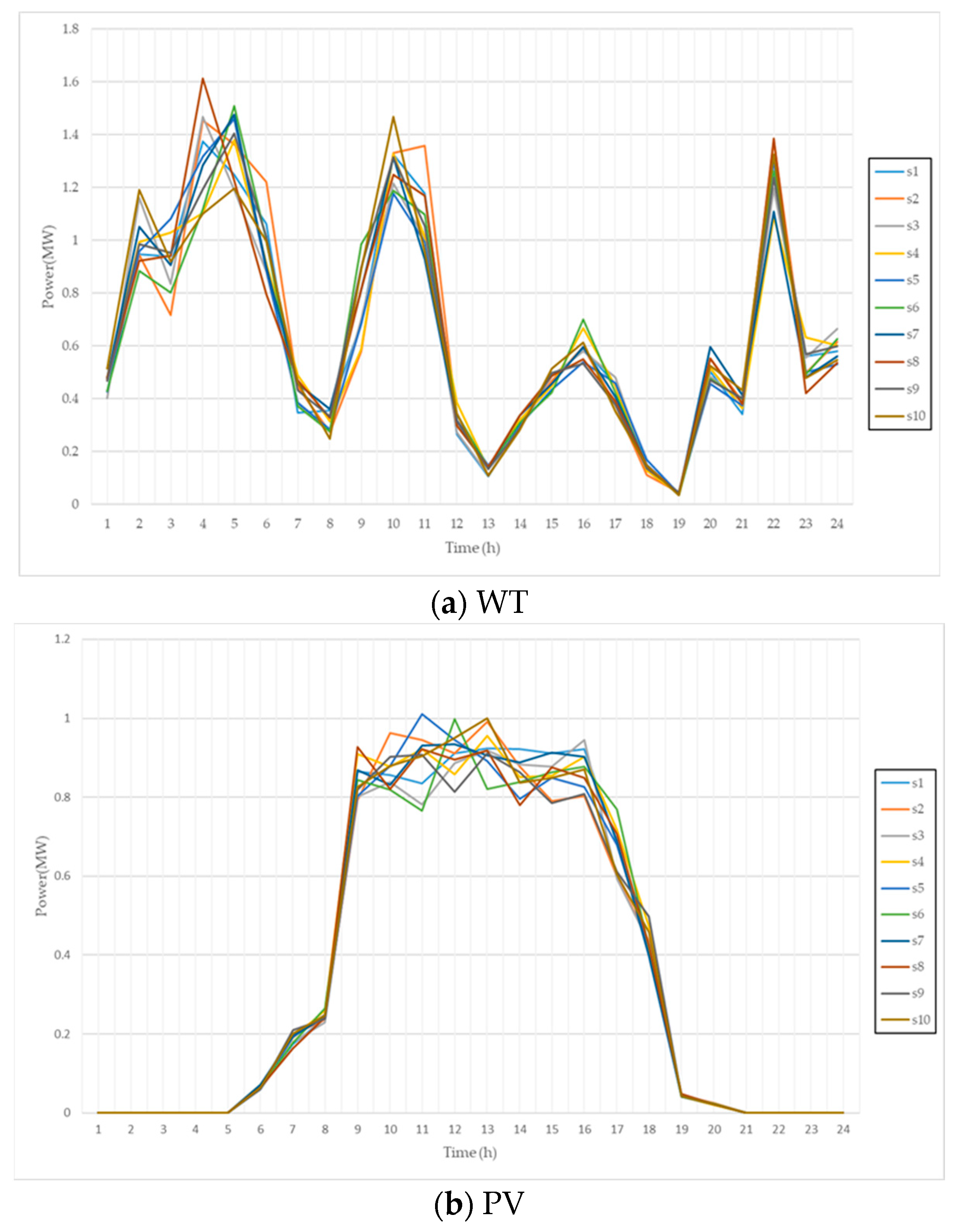
• Considering the uncertain characteristics of WTs, PVs, and load, historical data are generated through MCS based on the distribution function of each uncertain variable. The generated scenarios are reduced to cluster scenarios with a similar dense distribution through K-means clustering.
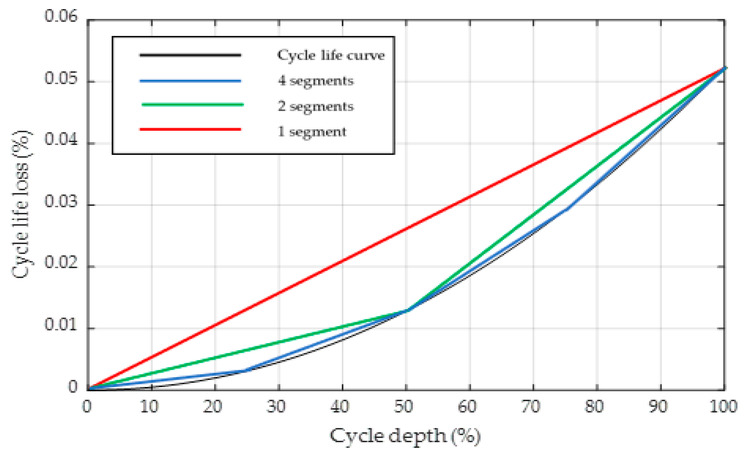
• Using the rainflow-counting algorithm, the SOC profile of the BESS is expressed as a charging/discharging cycle. By partially linearizing the nonlinear cycle aging stress function through linear approximation, the DOD cycle aging is formulated in the SUC problem.
• Using Benders decomposition (BD), the proposed optimal BESS scheduling is formulated as a master problem and a set of subproblems via parallel processing. In BD, the master problem solves SUC only through MILP without considering the BESS. The subproblem set derives the optimal operation scheduling considering the cycle aging of the BESS.
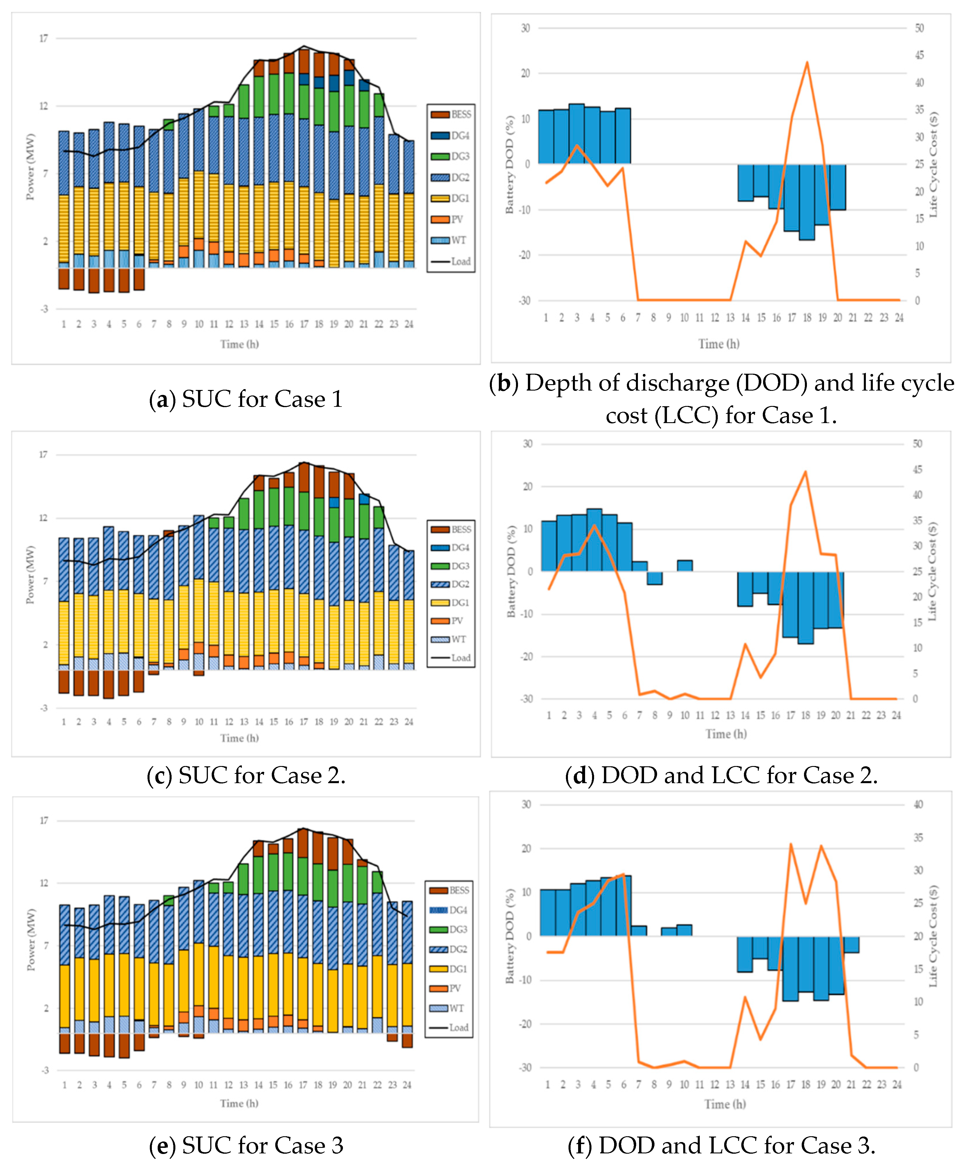
• The superiority of the proposed optimal BESS operation scheduling is shown by comparison with other cases. The simulation results confirm that the proposed scheduling is more effective at reducing the TOC and LCC simultaneously, while the life cycle of the BESS also increases significantly. Furthermore, by implementing BD, the convergence speed of the optimization process is improved in comparison with the cases without BD.

The remainder of this paper is organized as follows. Section 2 details the uncertainty modeling and analysis. Section 3 addresses BESS modeling, including the rainflow-counting algorithm and LCC. Section 4 models the proposed SUC problem considering the cycle aging of the BESS using BD. Section 5 provides the simulation results for different case studies, and Section 6 concludes the paper.

2. MG Modeling

Figure 1 shows the configuration of the MG system adopted in this study. It consists of diesel generators (DGs), WTs, PVs, loads, and a BESS. To solve the SUC problem, the amount of power generated by the RESs must be identified. To this end, we assume that the power generated by the WTs and PVs is known in advance from historical data, whereas the dispatchable output power units and the BESS operation are decision variables in the proposed SUC problem wind speeds, respectively.

2.1. Renewable Energy Sources Modeling

2.1.1. WT

Wind speed is a stochastic variable, and it is necessary to determine exactly how often or how strongly the wind blows to predict the output power of the WTs [29]. The wind energy at a particular wind speed can be expressed by the Weibull distribution:

$$f\left(v\right)=\frac{s}{h}{\left(\frac{v}{h}\right)}^{s-1}\exp \left(-{\left(\frac{v}{h}\right)}^s\right)$$

(1)

where h and s represent the distribution scale and shape parameters, respectively. h defines a measure of the characteristic wind speed of the distribution proportional to the average wind speed. s specifies the shape of the distribution and takes values between one and three. A small value of s represents a variable wind speed, while a constant wind speed is characterized by a larger value of s. The power output of a WT depends on the wind speed, and it can be calculated as follows:

$$P_{\mathrm{WT}}=\{\begin{array}{c}0\\ P_r\frac{v^3-v_{in}^3}{v_r^3-v_{in}^3}\\ P_r\end{array}\begin{array}{c}v{v}_{in} or v\ge v_{out}\\ v_{in}\le v{v}_r\\ v_r\le v{v}_{out}\end{array}$$

(2)

where $P_r$ and $v_r$ are the rated power and wind speed of the WT, respectively, and $v_{in}$and $v_{out}$ are the cut-in and cut-out.

2.1.2. PV

The power output of a PV generator depends on the power density, solar irradiation, and temperature [30]. The power output can be formulated as follows:

$$P_{\mathrm{PV}}\left(E_{\mathrm{M}}\right)=P_{\mathrm{STC}}\frac{n{E}_{\mathrm{M}}}{E_{\mathrm{STC}}}\left[1+k\left(T_{\mathrm{M}}-T_{\mathrm{STC}}\right)\right]$$

(3)

where $P_{\mathrm{PV}}$ is the output power of a PV plant, $P_{\mathrm{STC}}$ is the maximum power output of one module under test conditions, n is the number of modules in the plant, $E_{\mathrm{M}}$ is the incident irradiance on the modules, $E_{\mathrm{STC}}$ is the irradiance under standard test conditions (1000 W/${\mathrm{m}}^2$), k is the power-generation temperature coefficient of PVs (%/°C), $T_{\mathrm{M}}$ is the temperature of the module (°C), and $T_{\mathrm{STC}}$ is the reference temperature (25 °C).

2.1.3. Load

The stochastic characteristic of the load that causes uncertainty can be modeled as a normal probability density function (PDF) [31]:

$${\mathrm{PDF}}_{\mathrm{n}}\left(load\right)=\frac{1}{\sqrt{2\pi }\sigma }\exp \left(\frac{{(P_{load}-\mu )}^2}{2{\sigma }^2}\right)$$

(4)

For instance, the error may be adjusted to a normal distribution, which allows the application of the $3\mathsf{\sigma }$ criteria. This criterion provides a reliability band of 99.73%. Thus, the real value of the demand error will be in the width defined by $\left[{\mu }_{\mathrm{t}}-3{\sigma }_t, {\mu }_{\mathrm{t}}+3{\sigma }_t\right]$ in 99.73% of the cases.

2.2. Uncertainty Analysis Model

The WT, PV, and load models are described in Section 2.1. However, the values of their parameters may vary depending on the climate. Thus, it is necessary to predict such values accurately. Scenario generation is a procedure for selecting parameters, measurements, expected inputs, and disturbance to obtain the optimal solution for the MG. When this procedure is based on random sampling of scenarios created using MCS, it can be applied to solve problems involving normal and probability distributions of variables. Each scenario considers random WT and PV outputs and load per hour based on predicted values. The value of each parameter is determined by the probability of the scenario and can be divided by the number of net loads and preliminary scenarios according to the probability of the scenario. Each scenario represents the possible realization of a random process in the future.

In this study, according to the WT and PV outputs and random loads, 24 h scenarios were generated using MCS, while K-means clustering was adopted to reduce the scenario sets. K-means clustering is also known as least squares clustering [32]. Each scenario is described by its numerical features and represented as a data vector. Thus, a given number of cluster centers are searched to minimize the sum of squared distances from these vectors to the nearest center. Therefore, the original scenario can be reduced through the cluster scenario according to the cluster centers.

3. BESS Modeling

3.1. Operation Model

A BESS is considered indispensable for reliable MG operation because it provides security and flexibility to the system [33]. Given that a BESS can be used to balance renewable generation and load, it also reduces the operation cost by charging energy during the low-price period and discharging the stored energy during the high-price period, thereby reducing peak loads. We applied BESS operation scheduling to an MG configuration. When considering BESS operation, the SOC is the most important parameter for battery scheduling. It represents the amount of electricity stored in the battery. It is necessary to consider dynamic characteristics to perform detailed modeling of BESS charging and discharging. In this regard, the SOC of the BESS can be formulated as follows:

$$SO{C}_t=\{\begin{array}{c}SO{C}_{t-1}-\frac{P_{BESS,t}^{dch}M}{{\eta }_{BESS}^{dch}{E}_{BESS}^{rated}} \left(discharging\right)\\ SO{C}_{t-1}-\frac{P_{BESS,t}^{ch}{\eta }_{BESS}^{ch}M}{E_{BESS}^{rated}} \left(charging\right)\end{array}$$

(5)

where M is the duration of each period t; $E_{BESS}^{rated}$ is the rated capacity of the battery; $P_{BESS,t}^{dch}$ and $P_{BESS,t}^{ch}$ are the BESS discharging and charging power at time t, respectively; and ${\eta }_{BESS}^{ch} \mathrm{and} {\eta }_{BESS}^{dch}$ are the BESS charging and discharging efficiencies, respectively.

Due to the stochastic characteristics of the WTs, PVs, and loads, the BESS charging/discharging operation can be established in the MG. When the sum of RES outputs and power supplied by the DGs is greater than the load, the BESS is charged. Conversely, the BESS is discharged when the sum of WT and PV outputs and the power supply of the DGs are less than the load/demand. Accordingly, the BESS charging and discharging can be described as follows:

$${\displaystyle \sum }_i[P_{DG,i,t}+P_{WT,i,t}+P_{PV,i,t}]P_{load,t}$$

(6)

$${\displaystyle \sum }_i[P_{DG,i,t}+P_{WT,i,t}+P_{PV,i,t}]P_{load,t}$$

(7)

$$P_{BESS,t}=\{\begin{array}{c}{\eta }_{BESS}{P}_{ab}{P}_{BESS}^{rated}, \left|P_d\right|{\eta }_{BESS}{P}_{ab}{P}_{BESS}^{rated}\\ P_d, \left|P_d\right|\le {\eta }_{ESS}{P}_{ab}{P}_{BESS}^{rated}\end{array}$$

(8)

where $P_{ab}$ is the maximum absorbed power of the BESS; $P_d$ is the power deviation between the system and the stored energy, which can theoretically charge or discharge the BESS; ${\eta }_{BESS}$ is the battery charging/discharging efficiency; and $P_{BESS}^{rated}$ is the rated installation power of the BESS.

Equations (6) and (7) express the BESS charging and discharging conditions, respectively. Equation (8) represents the amount of BESS charging and discharging power with respect to the threshold value.

3.2. Life Cycle Aging Model

When considering a BESS for the SUC in MG operation, the battery’s lifetime cannot be assumed to be infinite. As the lifetime decreases, so does the battery performance. Therefore, replacement costs must be considered. In this regard, the assessment of the LCC of batteries should be considered. Battery aging consists of cycle and calendar aging. Cycle aging is the life lost due to battery cycles resulting from successive charging and discharging. The cycle aging, $L_{\mathrm{cyc}}$, is expressed as follows:

$$L_{\mathrm{cyc}}={\displaystyle \sum }_i^{\Gamma }{\gamma }_i{f}_c\left({\rho }_i,{\delta }_i,T_{c,i}\right)$$

(9)

where ${\delta }_i$ is the DOD of the ith cycle, ${\rho }_i$ is the average SOC of that cycle, $T_{c,i}$ denotes the average cell temperature, $\Gamma$ is the number of operation cycles, and ${\gamma }_i$ indicates whether cycle i is a full or half cycle.

We assume that each cycle is a single stress event. Thus, the degradation of the battery is the sum of the capacity reduction per cycle. Meanwhile, calendar aging represents the inherent degradation of the battery, which is affected by the battery’s temperature and SOC over a period [34]. Therefore, the calendar aging, $L_{cal}$, over a period t is expressed as a function of the SOC and cell temperature:

$$L_{cal}=f_t\left(t,\rho ,T_c\right)$$

(10)

where $L_{cyc}$ and $L_{cal}$ take into account the operational and non-operational factors, respectively.

Non-operational battery factors, such as temperature or number of days of use, might not be necessarily included during the operation phase [17]. Thus, $L_{cal}$ was not considered here because we only focused on indicating the LCC according to the BESS charging and discharging expressed in Equation (9).

3.2.1. Rainflow-Counting Algorithm

The rainflow-counting algorithm is applied for the stress analysis of materials in order to calculate the cumulative effect through cycle counting [35,36]. Here, this algorithm was adopted to assess the battery’s life cycle in the SUC problem of an MG. Figure 2 depicts the DOD provided by the rainflow-counting algorithm [37]. As an example, an SOC profile with local extremes ${\omega }_n$ is shown in Figure 2a. According to the rainflow-counting algorithm, the DOD can be calculated (as shown in Figure 2b) using the following sequence:

• The procedure starts from ${\omega }_0$ and involves the calculation of $\mathsf{\Delta }{\omega }_1=\left|{\omega }_0-{\omega }_1\right|, \mathsf{\Delta }{\omega }_2=\left|{\omega }_1-{\omega }_2\right|,$and $\mathsf{\Delta }{\omega }_3=\left|{\omega }_2-{\omega }_3\right|$;
• If $\mathsf{\Delta }{\omega }_2\le \mathsf{\Delta }{\omega }_1$ and $\mathsf{\Delta }{\omega }_2\le \mathsf{\Delta }{\omega }_3$, a full cycle of depth $\mathsf{\Delta }{\omega }_2$ is confirmed. Thereafter, ${\omega }_1 \mathrm{and} {\omega }_2$ are removed from the profile, and step (2) is repeated using points ${\omega }_0, {\omega }_3,{\omega }_4, {\omega }_5$…;
• If a cycle is not confirmed, the confirmation is shifted forward, and step (2) is repeated using points ${\omega }_1, {\omega }_2,{\omega }_3, {\omega }_4$…;
• The confirmation is repeated until no more full cycles can be confirmed throughout the remaining profile.

Figure 2. Cycle depths identified by the rainflow-counting algorithm.

Figure 2. Cycle depths identified by the rainflow-counting algorithm.

The remainder of the profile is only a half cycle, which has a pair of adjacent local extremes. As shown in Figure 2b, 10% and 20%, and 80% depths were identified in the charging and discharging cycles, respectively.

The cycle aging from a DOD, δ, is given by a polynomial cycle depth stress function Φ(δ) as follows:

$$L={\displaystyle \sum }_i^I\Phi \left({\delta }_i\right)$$

(11)

where L represents the total cycle aging, and Φ(δ) is a quadratic function with cycle depth δ.

The total aging of the BESS, L, from an SOC profile is calculated as the sum of cycle aging from confirmed cycles provided by the rainflow algorithm.

3.2.2. LCC

Batteries can reflect marginal operating costs. The marginal cost curve should reflect the cost due to battery performance degradation in each cycle [37,38]. To keep the model consistent and obtain a cost function, it is assumed that battery cycle aging occurs only during the discharge stage of the cycle. This is a reasonable assumption because, when assessing BESS scheduling daily, the amounts of charged and discharged energy from a BESS are equal.

During a cycle, if the BESS is discharged from a starting SOC to an end SOC and later charged back, the depth of the cycle is the difference in the SOC, where $E_{BESS}^{rated}$ is the energy capacity of the BESS. Let the battery be discharged from a cycle depth ${\delta }_{t-1}$ at time t−1. This cycle depth at time t can be identified from its output power $P_{BESS,t}^{dch}$ over time at 1 h intervals:

$${\delta }_t=\frac{P_{BESS,t}^{dch}}{{\eta }_{BESS}^{dch}{E}_{BESS}^{rated}}+{\delta }_{t-1}$$

(12)

$$\frac{\partial \Phi \left({\delta }_i\right)}{\partial P_{BESS,t}^{dch}}=\frac{d\Phi \left({\delta }_i\right)}{d{\delta }_i}\frac{\partial {\delta }_i}{\partial P_{BESS,t}^{dch}}=\frac{d\Phi \left({\delta }_t\right)}{d{\delta }_i}\frac{1}{{\eta }^{dch}{E}_{BESS}^{rated}}$$

(13)

The incremental aging resulting from this cycle is $\Phi \left({\delta }_t\right)$. The marginal cycle aging can then be calculated by taking the derivative of $\Phi \left({\delta }_t\right)$ with respect to $P_{BESS,t}^{dch}$ and substituting it in Equation (13). To determine the marginal cost of cycle aging, we assign a battery-cell replacement cost of R (USD) for marginal cycle aging and construct a piecewise linear approximation function c that consists of J segments, dividing the cycle depth evenly:

$$c\left({\delta }_t\right)=\{\begin{array}{c} c_1 if {\delta }_t\in \left[0,\frac{1}{J}\right) \\ ⋮\\ c_j if {\delta }_t\in \left[\frac{j-1}{J},\frac{j}{J}\right)\\ ⋮\\ c_J if {\delta }_t\in \left[\frac{J-1}{J},1\right]\end{array}$$

(14)

where

$$c_j=\frac{R}{{\eta }_{BESS}^{dch}{E}_{BESS}^{rated}}J\left[\Phi \left(\frac{j}{J}\right)-\Phi \left(\frac{j-1}{J}\right)\right]$$

(15)

The cycle depth $\delta$ at time t belongs to $c_j$, according to the present segment J, and $c_j$ is represented by a piecewise linear function about $\Phi$ through segment j.

Figure 3 illustrates the cycle depth stress function and its piecewise linearization with respect to the number of segments. The four lines indicate the original cycle life curve and its approximations according to the segments. The cycle life curve is similar to a quadratic curve that rapidly increases as the cycle depth $\delta$ increases. When the number of segments increases, the approximated line approaches the cycle life curve. To model the cycle depth in a multi-segment operation, we independently assign a charge power component $P_{BESS,t,j}^{dch}$ and an energy to each cycle depth segment to identify the current cycle depth.

For example, when a cycle of 10% depth starts with discharging, the BESS should undergo charging greater than 10% of the cycle depth, according to the rainflow-counting algorithm. Given that the marginal cost curve is convex, the BESS always discharges from the cheapest available cycle depth segment toward more expensive segments. The proposed optimization provides a close approximation to the algorithm.

4. Proposed SUC Optimization

In a compact form, the SUC model is described as follows:

$$\begin{array}{c}\underset{U,X}{min}f(Z)\hfill \\ s.t. G\left(X,U\right)=0\hfill \\ H_{min}\le H\left(X,U\right)\le H_{max}\hfill \end{array}$$

(16)

The sets G and H correspond to the equality and inequality constraints in the DG and BESS constraints, respectively.

The SUC model aims at minimizing the TOC of the generating units and the LCC of the BESS in the entire MG system, while considering the set of equations that define the system operational constraints.

4.1. Objective Function

The objective function involves minimizing the operation of the MG, including TOC and LCC:

$$f={\displaystyle \sum }_t{\displaystyle \sum }_i[F_i\left(P_{DG,i,t}\right)I_{i,t}+S{U}_{i,t}+S{D}_{i,t}]+{\displaystyle \sum }_t{\displaystyle \sum }_{j}M{c}_j{P}_{BESS,t,j}^{dch}$$

(17)

where $I_{i,t}$ is the commitment state of generator i at time t. $S{U}_{i,t}$ and $S{D}_{i,t}$ are the start-up and shut-down costs, respectively. $c_j$ is the marginal LCC of cycle depth segment j. $P_{BESS,t,j}^{dch}$ is the discharging power of cycle depth segment j at time t; and M represents the time interval.

Equation (17) describes the DG generation cost and LCC of the BESS. The first term involves the on/off states, fuel costs, and the start-up and shut-down costs of the ith generator at time t, while the second term includes the LCC cost and BESS output power. The LCC of the BESS is the sum of the cycle aging costs related to each segment over the period considered. The fuel cost is expressed as a quadratic function, as follows:

$$F_i\left(P_{DG,i,t}\right)=x_i+y_i\times P_{DG,i,t}+z_i\times P_{DG,i,t}^2$$

(18)

where $x_i, y_i,$ and $z_i$ are the fuel cost coefficients associated with each dispatchable unit.

4.2. System Constraints

4.2.1. Balancing Constraints

The total generated power from DGs, WTs, and PVs, and the BESS discharging power of the MG, should be equal to the total consumption. The BESS discharging power can be determined in accordance with optimal operating techniques:

$${\displaystyle \sum }_i\left[P_{DG,i,t}+P_{WT,i,t}+P_{PV,i,t}+P_{BESS,t}\right]=P_{load,t}$$

(19)

4.2.2. DG Constraints

The DG is subject to minimum and maximum generation capacity limits:

$$P_{DG,i,t}^{min}{I}_{i,t}\le P_{DG,i,t}\le P_{DG,i,t}^{max}{I}_{i,t}$$

(20)

Furthermore, it cannot ramp up or down beyond the ramp-rate constraints:

$$P_{DG,i,t}-P_{DG,i,t-1}\le U{R}_i$$

(21)

$$P_{DG,i,t-1}-P_{DG,i,t}\le D{R}_i$$

(22)

where $U{R}_i$ and $D{R}_i$ are the ramp-up and ramp-down rates of generator i, respectively.

When the generator is on, it is unable to generate below/over the up/down time limits:

$$T_{i,t}^{on}\ge U{T}_i\left(I_{i,t}-I_{i,t-1}\right)$$

(23)

$$T_{i,t}^{off}\ge D{T}_i\left(I_{i,t-1}-I_{i,t}\right)$$

(24)

where $T_{i,t}^{on}$ and $T_{i,t}^{off}$ are the time periods of start and stop at time t for generator i, respectively; $U{T}_i$ and $D{T}_i$ are the minimum up-time and maximum down-time of generator i, respectively.

4.2.3. RES Constraints

The generation capacity of WTs and PVs must be within the following limits:

$$P_{WT,t}^{min}\le P_{WT,t}\le P_{WT,t}^{max}$$

(25)

$$P_{PV,t}^{min}\le P_{PV,t}\le P_{PV,t}^{max}$$

(26)

4.2.4. BESS Constraints

The BESS constraints can be expressed as follows:

$$C={\displaystyle \sum }_t{\displaystyle \sum }_{j}M{c}_j{P}_{BESS,t,j}^{dch}$$

(27)

$$P_{ESS,t}^{ch}={\displaystyle \sum }_j{P}_{BESS,t,j}^{ch}$$

(28)

$$P_{ESS,t}^{dch}={\displaystyle \sum }_j{P}_{BESS,t,j}^{dch}$$

(29)

$$e_{t,j}-e_{t-1,j}=M(P_{BESS,t,j}^{dch}{\eta }^{ch}-\frac{P_{BESS,t,j}^{dch}}{{\eta }^{dch}})$$

(30)

$$e_{t,j}\le {\overline{e}}_j$$

(31)

$$E^{min}\le {\displaystyle \sum }_j{e}_{t,j}\le E^{max}$$

(32)

$$e_{1,j}=e_j^0$$

(33)

$${\displaystyle \sum }_t{\displaystyle \sum }_j{e}_{t,j}\ge E^{final}$$

(34)

where $e_{t,j}$ is the energy stored in marginal cost segment j at time t; ${\overline{e}}_j$ is the maximum amount of energy that can be stored in cycle depth segment j; $E^{min}$ and $E^{max}$ represent the minimum and maximum energy stored in the BESS, respectively; $e_j^0$ is the initial amount of energy of segment j; and $E^{final}$ is the amount of energy stored at the end of the scheduling horizon.

Equation (27) is the sum of the LCC associated with each segment over the horizon. Equations (28) and (29) represent the equivalent charging power and discharging power, respectively. Equation (30) is the amount of energy stored in each cycle depth segment, considering charging and discharging efficiencies. Equation (31) represents the upper limit of each segment. Equation (32) limits the minimum and maximum SOC of the BESS. Equation (33) sets the initial stored energy in each cycle depth segment. The final storage energy level is described by Equation (34).

4.3. Benders Decomposition

When solving a conventional UC problem for MG operation, the BESS has not been widely considered in the optimization process to date. However, by incorporating the BESS in such a process, the scheduling results of existing DGs change, and the operating cost varies accordingly. By applying the BESS in the SUC of an MG, the aforementioned objective function was adopted to minimize the operating cost of the DGs and the LCC of the BESS. However, it is complicated to solve the optimization problem of minimization for both the TOC and LCC while considering the uncertainty and BESS simultaneously. In addition, convergence issues can arise when solving an MILP problem. To this end, BD was applied to solve the stochastic UC problem of the MG more effectively by dividing it into a master problem and subproblems. Figure 4 shows the BD process to solve the optimization problem. First, the SUC of the base case, without considering the BESS, is obtained. Then, the BESS schedule is acquired, and restrictions are added following violations of the BESS operations. If violations no longer exist, the Benders cut is added until the BESS operation is feasible.

4.3.1. Subproblem

A subproblem addresses the operation constraints of the BESS, formulated in Equations (27)–(34). The objective function of subproblem $S_a\left(u_o\right)$can be formulated as follows:

$$\begin{array}{c}{S}_a\left(u_o\right)=Max {\displaystyle {\displaystyle \sum }_i}\left(s_n-C_n\right) \hfill \\ \hspace{1em}s.t. G_n\left(X_n, U_n\right)=0, n=1, 2, \dots , N\hfill \\ \hspace{1em}\hspace{1em}\hspace{1em}\hspace{1em}{H}_n^{min}\le H_n\left(X_n, U_n\right)\le H_n^{max}, n=1, 2, \dots , N \hfill \\ \hspace{1em}\hspace{1em}{\delta }_n\le {\delta }_m, n=1, 2, \dots , N \hfill \end{array}$$

(35)

where $s_n$ denotes a reduction in power generation costs through BESS, and $C_n$ represents the cycle aging costs of the BESS.

According to Equation (35), the objective function of the subproblem can be expressed as the maximum profit when applying the BESS. The first and second constraints represent the equality and inequality constraints of the subproblem objective function, respectively. Given that ${\delta }_m$ is the marginal depth of charge, ${\delta }_n$ cannot be higher than ${\delta }_m$. In other words, if the depth of charge is higher than ${\delta }_m$, the cost is higher than the savings achieved from the BESS scheduling. Thus, the subproblem is feasible through this DOD constraint, which is added to the master problem as a Benders cut.

4.3.2. Master Problem

The master problem is formulated as Equations (30)–(34), and the constraints are updated by Benders cuts. In the master problem, the optimization problem is expressed as follows:

$$\begin{gathered} Min S\left(U_0\right)={\displaystyle \sum }_t{\displaystyle \sum }_i[F_i\left(P_{DG,i,t}\right)I_{i,t}+S{U}_{i,t}+S{D}_{i,t}]+{\displaystyle \sum }_t{\displaystyle \sum }_{j}M{c}_j{P}_{BESS,t,j}^{dch} \\ st. G\left(X_0,U_0\right)=0 \\ {H}_{min}\le H\left(X_0,U_0\right)\le H_{max} \\ {S}_a\left(u_0\right)\le 0 \end{gathered}$$

(36)

The last constraint defined in Equation (35) is referred to as a Benders cut. This is a linear constraint that limits the feasible area to adjust the coordination of the solutions of the master problem and subproblems. The Benders cut is generated by the DOD constraint of the subproblem, which is applied to the master problem according to the BESS charging/discharging schedule. This indicates that it can be accepted as the updated generating volume profile of the master problem. After receiving an updated generating volume profile, the master problem repeats the iteration process by sending the on/off status and power generation data of the generator to subproblems according to the SUC results. It should be noted that $S_a\left(u_0\right)=0$ represents the feasible cost result of the scenarios, while $S_a\left(u_0\right)0$ implies that the scenario’s result is not feasible.

4.4. Solution Procedure

Figure 5 illustrates the process of the optimal BESS operation scheduling for SUC problems. The overall procedure can be implemented sequentially:

Step 1:

Set the DG, PV, WT, load, and BESS data;

Step 2:

Following the error of elements, generate each WT, PV, and load scenario using MCS and obtain the representative scenarios according to K-means clustering;

Step 3:

Solve the SUC problem by implementing BD.

(a)

Compute the base case of the SUC problem (master problem), which does not consider the BESS constraints, through MILP.

(b)

Apply BESS to maximize the MG revenue.

(b1)

Configure the BESS charging/discharging schedule according to generating volumes and power generation (subproblem).

(b2)

Calculate the LCC of the BESS using the rainflow-counting algorithm and linear approximation.

(b3)

Derive the LCC of the BESS.

(b4)

Add Benders cut to the master problem according to the DOD.

Step 4:

Return to Step 3 until the last scenario is solved.

Figure 5. Overall process of optimal BESS operation scheduling.

Figure 5. Overall process of optimal BESS operation scheduling.

5. Case Studies

Dataset of MG

To improve the operational efficiency of the MG, the proposed optimal BESS scheduling was based on stochastic parameters. An MG test system described in ref. [39] was used to analyze the proposed SUC model. It consists of four DGs, one WT, one PV, and one BESS.

Table 1. Technical data of generating units.

Sources	Cost Coefficient (USD/MWh)	${\mathit{P}}_{\mathit{m}\mathit{i}\mathit{n}} \left(\mathbf{MW}\right)$	${\mathit{P}}_{\mathit{m}\mathit{a}\mathit{x}} \left(\mathbf{MW}\right)$	$\mathit{R}\mathit{U} (\mathbf{MW}/\mathbf{h})$	$\mathit{R}\mathit{D} (\mathbf{MW}/\mathbf{h})$	Minimum Up/Down Time (h)
DG 1	27.7	1	5	2.5	2.5	3
DG 2	39.1	1	5	2.5	2.5	3
DG 3	61.3	0.8	3	3	3	1
DG 4	65.6	0.8	3	3	3	1
WT	0	0	1.5	-	-	-
PV	0	0	1	-	-	-

depicts the technical parameters of the MG generation units. The DG parameters correspond with relatively inexpensive cost coefficients and large capacities. However, DGs 3 and 4 have a higher cost coefficient and a smaller capacity. Therefore, DGs 1 and 2 are responsible for the base load, whereas DGs 3 and 4 are suitable for the peak load. The maximum power outputs of the WTs and PVs were set as 1.5 MW and 1 MW, respectively.

Table 2. BESS test parameters.

BESS Parameters	Value
Charging and discharging power rating	3 MW
Energy capacity	15 MWh
Charging and discharging efficiency	95%
Maximum SOC	90%
Minimum SOC	10%
Battery replacement cost	300,000 USD/MWh

shows the adopted test parameters for the BESS. The battery has a life span of 3000 cycles when operated at 80% DOD, and the life cycle also changes as the depth of the cycle changes. It can charge or discharge 3 MW/h with a maximum and minimum SOC of 90% and 10%, i.e., 13.5 MWh and 1.5 MWh, respectively. The battery cells have a near-quadratic stress function:

$$\Phi \left(\delta \right)=\left(5.24\times {10}^{-4}\right){\delta }^{2.03}$$

(37)

Figure 6 depicts the initial 24 h forecast data for the uncertain inputs. The data are assumed to be extracted from independent random processes based on historical values. The time horizon of scheduling for this simulation were 1 h intervals over one day. The SUC problem was implemented using MATLAB simulation (scripts).

To address uncertain variables effectively, scenarios were generated through MCS considering certain PDFs. These scenarios were then reduced to cluster scenarios through K-means clustering. Figure 7 shows the input data for WTs, PVs, and load. Here, we have generated 1000 scenarios for each stochastic case. The scenario generation for WTs, PVs, and load was computed as a randomized forecasting error. According to Weibull and standard distributions, each scenario has its own probability of occurrence. Depending on the distribution, the scenarios of uncertainties represented by data vectors are reduced to 10 cluster scenarios by determining the cluster center.

To demonstrate the superiority of the proposed optimal BESS operation scheduling, four case studies were considered. Thereafter, the SUC problem was solved for these cases. The objective function was applied differently with respect to each scheduling case. In the base case, the BESS was not considered in MG operation. This case is the basis for elucidating the cost-saving effects of the other cases. In Case 1, the SUC problem has been solved with power-generation cost reduction, without considering the cycle aging of the BESS. In Case 2, optimization was performed by linearizing the convex cycle-depth aging-stress function of the BESS. In other words, this case included the assumption that the cycle aging of the BESS increases according to the sum of all DODs in the scheduling problem. Finally, in Case 3, the proposed operation scheduling that optimizes BESS operation with both cycle aging and power generation units was applied.

Figure 8 shows the SUC results for the base case computed without considering BESS utilization. It should be noted that the DG with the lowest generation cost was assigned the highest priority. Thus, DG4 operated between 14 and 21 h, which was when the peak load occurred.

Figure 9 shows the scheduling results of the SUC and BESS scheduling for Cases 1, 2, and 3. In Case 1, BESS has been applied to reduce the peak load with respect to the base case. DG4’s power generation was reduced by charging the BESS when the charging price was low. While DG2’s power-generation capacity was available, the peak load has been reduced by discharging the BESS when DG4 was on. Figure 9b depicts the battery DOD with respect to the amount of change in the SOC. Figure 9c,d show the BESS operation scheduling results considering the peak shaving of the BESS and the battery’s life cycle. By linearizing the convex aging stress function of the BESS, operation scheduling has been optimized on the premise that the battery’s life cycle decreases owing to the sum of the DOD in the scheduling problem, regardless of each DOD size. Figure 9e,f illustrate the proposed BESS operation scheduling considering both the peak shaving and the BESS life cycle, as in Case 2. However, unlike Case 2, the cycle-depth aging-stress function is piecewise linearized. Consequently, Case 3 shows the cycle life loss more accurately. Notably, this indicates that cycle aging can be minimized.

Figure 10 depicts the characteristics of the BESS for each case. The battery SOC profiles are shown in Figure 10a. As indicated by this curve, there exists a base load between 0 and 6 h and a peak load between 14 and 20 h. The SOC curve of Case 1 represents charging to the maximum SOC (90%) under the base load and then discharging during peak-load periods when the most expensive generator is operating. Meanwhile, the SOC curve of Case 2 shows that the charging and discharging processes are more rapid than those of Case 1. Case 3 has a curve similar to Case 1; however, the BESS charges or discharges more smoothly than in Case 1. A slight difference in the curve indicates a significant effect on the LCC, because the cycle life loss of the battery increases rapidly with a small increase in DOD. Figure 10b depicts the cycle life loss according to the operation scheduling of Cases 1, 2, and 3. It is evident that the cycle life loss increases sharply during the charging period between 1 and 6 h and the discharging period between 16 and 20 h. The cycle life loss in Case 3 is the lowest, 0.00138% per day, which is approximately 10% lower than that in the other cases.

Table 3. Comparison of costs in all cases.

Case	Generating Cost (USD)	LCC (USD)	TOC (USD)	Lifetime (Days)	Savings (%)
Base	10,072	0	10,072	-	0
1	9736.7	328.6	10,065.3	2880	0.067
2	9783.5	272.8	10,056.3	2930	0.156
3	9722.9	256.7	9979.6	3260	0.918

shows the overall cost comparison for all the cases. In Case 1, cycle aging of the battery was not considered, but there was no significant difference in the TOC. Compared with Case 1, Case 2 slightly reduced the LCC by linearizing the aging stress function of the battery. The generation cost and LCC in Case 3 were USD 9722.9 and USD 256.7, respectively, with a TOC of USD 9979.6. This represents the lowest value among all the cases, and the lifetime of BESS was approximately 300 days longer than that in the other cases. Compared to the other cases, presenting insignificant savings, Case 3 shows a remarkable result. Finally, Case 3 notably increased the lifetime of the BESS while reducing the TOC of the MG, in comparison with the other cases, by considering the actual life cycle loss of the BESS.

Table 4. Comparison of iterations in all cases.

Case	Iterations (w/o BD)	Iterations (with BD)	Ratio
1	17	14	0.82
2	16	13	0.84
3	25	16	0.64

shows the comparison of the number of iterations with respect to the application of BD. While BD was not used, Case 3 iterated nearly 50% more than Cases 1 and 2. This is due to the complicated approach of Case 3. However, while BD was used, Case 3 presented a very similar value in comparison with Cases 1 and 2. This implies that the convergence speed of complex calculations can be significantly improved. According to the ratio between the results without and with BD, Case 3 showed the highest performance. The parallel processing nature of BD should be noted; these results indicate that the calculation speed can be improved as the number of uncertainties increases, and that a more realistic power system which readily matches the requirements of realistic day-ahead BESS scheduling is achieved. Likewise, when considering a more realistic power system with more uncertain variables, optimal operation scheduling with BD could further improve computational efficiency.

6. Conclusions

In this study, optimal scheduling of MGs with BESSs was proposed to solve the SUC problem, considering the uncertainties of WTs, PVs, and the load. In particular, to minimize the TOC of the MG, we focused on operation scheduling that minimizes the life degradation of BESSs. To solve the SUC problem of the MG, scenario generation was implemented based on MCS. To improve the computational efficiency of the optimization problem, the scenarios were reduced via K-means clustering. In the proposed BESS scheduling, the SOC profile of the BESS was converted into a charging/discharging cycle using the rainflow-counting algorithm. Cycle aging was linearly approximated using the partially linearized aging stress function. The formulation of the proposed scheduling problem was divided into a master problem and subproblems by adopting BD to improve computational efficiency through parallel processing. In the master problem, the SUC problem was solved, while the subproblems optimized the BESS charging/discharging scheduling problem. The simulation results revealed that the proposed BESS scheduling exhibited superiority in terms of economic operation, and TOC and LCC decreased in comparison with other cases. This indicates that the MG as well as industry and community can operate BESSs with a significantly longer lifetime compared to other cases for the same investment cost. In addition, the comparative analysis with and without BD revealed that the iteration for convergence was also significantly reduced in the proposed optimal BESS scheduling. From the perspective of the MG operator, one of the primary goals is to reduce operation costs. To this end, the use of BESSs is essential, and these results can assist the MG operator in decision-making when achieving MG operation with reduced TCC and LCC with advanced computational efficiency. In future research, we plan to apply BESS scheduling to a real MG system to demonstrate the applicability and effectiveness of the proposed BESS scheduling.

References

1. Soshinskaya, M.; Crijns-Graus, W.H.; Guerrero, J.M.; Vasquez, J.C. Microgrids: Experiences, barriers and success factors. Renew. Sustain. Energy Rev. 2014, 40, 659–672. [Google Scholar] [CrossRef] [Green Version]
2. Wang, J.; Xu, Y.; Lv, M. Modeling and Simulation Analysis of Hybrid Energy Storage System Based on Wind Power Generation System. In Proceedings of the 2018 International Conference on Control, Automation and Information Sciences (ICCAIS), Hangzhou, China, 24–27 October 2018; Institute of Electrical and Electronics Engineers (IEEE): Piscataway, NJ, USA, 2018; pp. 422–427. [Google Scholar]
3. Divya, K.; Østergaard, J. Battery energy storage technology for power systems—An overview. Electr. Power Syst. Res. 2009, 79, 511–520. [Google Scholar] [CrossRef]
4. Oudalov, A.; Cherkaoui, R.; Beguin, A. Sizing and Optimal Operation of Battery Energy Storage System for Peak Shaving Application. In 2007 IEEE Lausanne Power Tech; Institute of Electrical and Electronics Engineers (IEEE): Piscataway, NJ, USA, 2007; pp. 621–625. [Google Scholar]
5. Zhao, B.; Zhang, X.; Chen, J.; Wang, C.; Guo, L. Operation Optimization of Standalone Microgrids Considering Lifetime Characteristics of Battery Energy Storage System. IEEE Trans. Sustain. Energy 2013, 4, 934–943. [Google Scholar] [CrossRef]
6. Sheble, G.B.; Fahd, G.N. Unit commitment literature synopsis. IEEE Trans. Power Syst. 1994, 9, 128–135. [Google Scholar] [CrossRef]
7. Jabbari-Sabet, R.; Moghaddas-Tafreshi, S.-M.; Mirhoseini, S.-S. Microgrid operation and management using probabilistic reconfiguration and unit commitment. Int. J. Electr. Power Energy Syst. 2016, 75, 328–336. [Google Scholar] [CrossRef]
8. Siahkali, H.; Vakilian, M. Stochastic unit commitment of wind farms integrated in power system. Electr. Power Syst. Res. 2010, 80, 1006–1017. [Google Scholar] [CrossRef]
9. Jo, K.-H.; Kim, M. Stochastic Unit Commitment Based on Multi-Scenario Tree Method Considering Uncertainty. Energies 2018, 11, 740. [Google Scholar] [CrossRef] [Green Version]
10. Kim, H.; Kim, M.; Lee, J. A two-stage stochastic p-robust optimal energy trading management in microgrid operation considering uncertainty with hybrid demand response. Int. J. Electr. Power Energy Syst. 2021, 124, 106422. [Google Scholar] [CrossRef]
11. Bruninx, K.; Delarue, E. Scenario reduction techniques and solution stability for stochastic unit commitment problems. In Proceedings of the 2016 IEEE International Energy Conference (ENERGYCON), Leuven, Belgium, 4–8 April 2016; Institute of Electrical and Electronics Engineers (IEEE): Piscataway, NJ, USA, 2016; pp. 1–7. [Google Scholar]
12. Olivares, D.E.; Canizares, C.A.; Kazerani, M. A Centralized Energy Management System for Isolated Microgrids. IEEE Trans. Smart Grid 2014, 5, 1864–1875. [Google Scholar] [CrossRef]
13. Farhadi, M.; Mohammed, O. Energy Storage Technologies for High-Power Applications. IEEE Trans. Ind. Appl. 2016, 52, 1953–1961. [Google Scholar] [CrossRef]
14. Zhang, Z.; Wang, J.; Wang, X. An improved charging/discharging strategy of lithium batteries considering depreciation cost in day-ahead microgrid scheduling. Energy Convers. Manag. 2015, 105, 675–684. [Google Scholar]
15. Kim, R.-K.; Glick, M.B.; Olson, K.R.; Kim, Y.-S. MILP-PSO Combined Optimization Algorithm for an Islanded Microgrid Scheduling with Detailed Battery ESS Efficiency Model and Policy Considerations. Energies 2020, 13, 1898. [Google Scholar] [CrossRef] [Green Version]
16. Alvarado-Barrios, L.; Del Nozal, Á.R.; Valerino, J.B.; Vera, I.G.; Martínez-Ramos, J.L. Stochastic unit commitment in microgrids: Influence of the load forecasting error and the availability of energy storage. Renew. Energy 2020, 146, 2060–2069. [Google Scholar] [CrossRef]
17. He, G.; Chen, Q.; Kang, C.; Pinson, P.; Xia, Q. Optimal Bidding Strategy of Battery Storage in Power Markets Considering Performance-Based Regulation and Battery Cycle Life. IEEE Trans. Smart Grid 2016, 7, 2359–2367. [Google Scholar] [CrossRef] [Green Version]
18. Dong, X.; Yuying, Z.; Tong, Z. Planning-operation co-optimization model of active distribution network with energy storage considering the lifetime of batteries. IEEE Access 2018, 6, 59822–59832. [Google Scholar] [CrossRef]
19. Xu, B.; Oudalov, A.; Ulbig, A.; Andersson, G.; Kirschen, D.S. Modeling of Lithium-Ion Battery Degradation for Cell Life Assessment. IEEE Trans. Smart Grid 2018, 9, 1131–1140. [Google Scholar] [CrossRef]
20. Motapon, S.N.; Lachance, E.; Dessaint, L.A.; Al-Haddad, K. A Generic Cycle Life Model for Lithium-Ion Batteries Based on Fatigue Theory and Equivalent Cycle Counting. IEEE Open J. Ind. Electron. Soc. 2020, 1, 207–217. [Google Scholar] [CrossRef]
21. Alam, M.J.E.; Saha, T.K. Cycle-life degradation assessment of Battery Energy Storage Systems caused by solar PV variability. In Proceedings of the 2016 IEEE Power and Energy Society General Meeting (PESGM), Boston, MA, USA, 17–21 July 2016; Institute of Electrical and Electronics Engineers (IEEE): Piscataway, NJ, USA, 2016; pp. 1–5. [Google Scholar]
22. Eom, J.-K.; Noh, Y.-S.; Lee, S.-R.; Choi, B.-Y.; Won, C.-Y. ESS operation algorithm for economics considering battery degradation properties. In Proceedings of the 2014 IEEE Conference and Expo Transportation Electrification Asia-Pacific (ITEC Asia-Pacific), Beijing, China, 31 August–3 September 2014; Institute of Electrical and Electronics Engineers (IEEE): Piscataway, NJ, USA, 2014; pp. 1–5. [Google Scholar]
23. Choi, Y.; Kim, H. Optimal Scheduling of Energy Storage System for Self-Sustainable Base Station Operation Considering Battery Wear-Out Cost. Energies 2016, 9, 462. [Google Scholar] [CrossRef] [Green Version]
24. Kim, H.; Kim, M. Optimal generation rescheduling for meshed AC/HIS grids with multi-terminal voltage source converter high voltage direct current and battery energy storage system. Energy 2017, 119, 309–321. [Google Scholar] [CrossRef]
25. Fan, H.; Yuan, Q.; Cheng, H. Multi-Objective Stochastic Optimal Operation of a Grid-Connected Microgrid Considering an Energy Storage System. Appl. Sci. 2018, 8, 2560. [Google Scholar] [CrossRef] [Green Version]
26. Uddin, M.; Romlie, M.F.; Abdullah, M.; Tan, C.; Shafiullah, G.; Bakar, A. A novel peak shaving algorithm for islanded microgrid using battery energy storage system. Energy 2020, 196, 117084. [Google Scholar] [CrossRef]
27. Alamri, A.; AlOwaifeer, M.; Meliopoulos, A.P.S. Multi-Objective Unit Commitment Economic Dispatch for Power Systems Reliability Assessment. In Proceedings of the 2020 International Conference on Probabilistic Methods Applied to Power Systems (PMAPS), Liege, Belgium, 18–21 August 2020; Institute of Electrical and Electronics Engineers (IEEE): Piscataway, NJ, USA, 2020; pp. 1–6. [Google Scholar]
28. Vatanpour, M.; Yazdankhah, A.S. The impact of energy storage modeling in coordination with wind farm and thermal units on security and reliability in a stochastic unit commitment. Energy 2018, 162, 476–490. [Google Scholar] [CrossRef]
29. Eisenhut, C.; Krug, F.; Schram, C.; Klckl, B. Wind-Turbine Model for System Simulations Near Cut-In Wind Speed. IEEE Trans. Energy Convers. 2007, 22, 414–420. [Google Scholar] [CrossRef]
30. Tsai, H.L.; Tu, C.S.; Su, Y.J. Development of generalized photovoltaic model using MATLAB/SIMULINK. In Proceedings of the World Congress on Engineering and Computer Science, San Francisco, CA, USA, 22–24 October 2008; Volume 2008. [Google Scholar]
31. He, S.; Yang, S.; Cao, X.; Lu, Z.; Zhang, H.; Wei, Z. Short-term Power Load Probability Density Forecasting Based on PCA-QRF. In Proceedings of the 2018 2nd IEEE Conference on Energy Internet and Energy System Integration (EI2), Beijing, China, 20–22 October 2018; Institute of Electrical and Electronics Engineers (IEEE): Piscataway, NJ, USA, 2018; pp. 1–5. [Google Scholar]
32. Ryu, H.-S.; Kim, M. Two-Stage Optimal Microgrid Operation with a Risk-Based Hybrid Demand Response Program Considering Uncertainty. Energies 2020, 13, 6052. [Google Scholar] [CrossRef]
33. Sarker, M.R.; Murbach, M.D.; Schwartz, D.T.; Ortega-Vazquez, M.A. Optimal operation of a battery energy storage system: Trade-off between grid economics and storage health. Electr. Power Syst. Res. 2017, 152, 342–349. [Google Scholar] [CrossRef]
34. Ecker, M.; Nieto, N.; Käbitz, S.; Schmalstieg, J.; Blanke, H.; Warnecke, A.; Sauer, D.U. Calendar and cycle life study of Li (NiMnCo) O2-based 18650 lithium-ion batteries. J. Power Sources 2014, 248, 839–851. [Google Scholar] [CrossRef]
35. Musallam, M.; Johnson, C.M. An Efficient Implementation of the Rainflow Counting Algorithm for Life Consumption Estimation. IEEE Trans. Reliab. 2012, 61, 978–986. [Google Scholar] [CrossRef]
36. Lee, Y.L.; Barkey, M.E.; Kang, H.T. Metal Fatigue Analysis Handbook: Practical Problem-Solving Techniques for Computer-Aided Engineering; Elsevier: Amsterdam, The Netherlands, 2011. [Google Scholar]
37. Xu, B.; Zhao, J.; Zheng, T.; Litvinov, E.; Kirschen, D.S. Factoring the cycle aging cost of batteries participating in electricity markets. IEEE Trans. Power Syst. 2017, 33, 2248–2259. [Google Scholar]
38. Weitzel, T.; Schneider, M.; Glock, C.H.; Löber, F.; Rinderknecht, S. Operating a storage-augmented hybrid microgrid considering battery aging costs. J. Clean. Prod. 2018, 188, 638–654. [Google Scholar] [CrossRef]
39. Khodaei, A. Microgrid Optimal Scheduling With Multi-Period Islanding Constraints. IEEE Trans. Power Syst. 2013, 29, 1383–1392. [Google Scholar] [CrossRef]
Figure 1. Proposed structure of MG.
Energies 14 00470 g001
Figure 3. Approximations of the cycle depth aging stress function.
Energies 14 00470 g003
Figure 4. Benders decomposition.
Energies 14 00470 g004
Figure 6. Forecasted input data.
Energies 14 00470 g006aEnergies 14 00470 g006b
Figure 7. Cluster scenarios of uncertainties for 24 h.
Energies 14 00470 g007aEnergies 14 00470 g007b
Figure 8. SUC results for base case.
Energies 14 00470 g008
Figure 9. Scheduling results for each case.
Energies 14 00470 g009
Figure 10. Battery characteristic for each case.
Energies 14 00470 g010