Abstract
A new robust scheduling method for pumping water in a water distribution system under the uncertainty of activating regulation reserves is proposed in this paper. During the operation of power systems, utilizing the energy equipment of the customer to enhance supply-demand control is attracting attention. Because water pumps have been already installed, they can be regarded as a relatively inexpensive, operational, and flexible resource. Changes in the operation of the water pump can contribute to the power supply and demand control. The proposed method helps generate a robust daily schedule for pumping water and provides regulation reserves under the uncertainty of activating regulation reserves. It is based on electric energy prices and regulation reserves, hourly water demand profiles, and the properties of water flow quantity and the electricity consumption of water pumps. This method comprises an optimization model formulated using mixed integer linear programming, validated through simulations of water pumping scheduling under certain scenarios. The results indicate that the net operational cost decreased when water pumps provided regulation reserves; further, the operational feasibility of providing these reserves from water pumps is clarified. The proposed model makes it possible to optimize power system operation that integrates the water supply system.
1. Introduction
Water supply is an essential public infrastructure in modern society. The electricity consumption of water supply projects in Japan accounts for about 1% of the annual electricity consumption of the country [1]. Among these projects, the share of electricity consumption by water supply facilities, especially pumps, is the highest. Therefore, the New Water Supply Vision formulated by the Ministry of Health, Labour and Welfare (MHLW) in 2013 [2] recommends energy-saving measures for water supply facilities, and thus, each municipality has created its own water supply vision. In the United States, the high energy cost related to the power consumption of pumps in water supply has become a concern [3]. In response to these social demands for energy conservation and energy cost reduction, energy management methods for water supply systems have been proposed [4,5,6,7,8,9,10,11,12,13,14,15].
One of the difficulties in optimizing the energy management of water supply systems is that the power consumption characteristics of the water pumps are non-linear. If the non-linear characteristics of water pumps are treated in the optimization problem, it is modeled as a mixed integer non-linear programming (MINLP), which cannot be solved by general optimizing solvers. Therefore, methods using by meta-heuristics [6,7,8] and a branch and bound algorithm [9,10] have been proposed to solve the problem. The optimization models have been proposed to solve for the non-linear characteristics of the water pumps as mixed integer linear programming (MILP) by linear relaxation [4,5,12].
An optimization model was proposed to determine the water pump operation where daily power consumption is minimized by modeling it as an MILP [4]. The characteristics of the power consumption for non-linear pump flow rates are approximated by a piecewise linear function divided into two value ranges. An optimization model was proposed for water pump operation with demand response (DR) using the water pump [5]. An energy cost minimization model in the time-of-day rate system was obtained by combining a water supply simulator, EPANET [16], proposed in [6]. In [11], the authors proposed an optimization model for water pump operation, including the start-up and shut-down costs of water pumps and the physical constraints of the water distribution network. Further, it was modeled as an optimization problem that minimizes the objective function, which is the energy cost minus the incentive by DR, assuming incentive DR. In [12], an optimization model was proposed wherein water pump operational planning was modeled as an MILP, and it is robust to the error in the predicted value of the water demand at each time. The characteristics of power consumption with respect to the pump flow rate are studied using piecewise linear regression to extract an efficient pump operation pattern and to linearize the characteristics of water pumps. In [13], a facility-scale optimization problem, including the operation of water treatment plants and pumps, formulated as an MILP, was proposed. The model was used to evaluate the potential cost savings of the water distribution system providing flexibility to the power systems. In [14], the model included the physical constraints of the water distribution network. Further, an optimization model was proposed that minimizes the energy loss of water caused by water distribution using a cost function weighted by the price of electricity as the objective function. A method for determining the operation of pumps installed in the water distribution network in a Markov decision process was also proposed [15].
Thus, various optimization models have been proposed for the energy management of water distribution systems in water supply. In recent years, commercial solvers such as the Gurobi Optimizer [17] and CPLEX [18], which can rapidly solve MILPs fast, have become more widely available, and modeling with MILPs [4,5,12] is considered highly versatile and practical.
The penetration of variable renewable energy (VRE) power sources such as photovoltaic (PV) and wind power (WP) has been progressing rapidly. The output of PVs and WP fluctuates because of changing weather conditions such as solar radiation and wind speed; therefore, supply and demand are matched by increasing or decreasing the output of the thermal power units in accordance with the VRE output fluctuations. When the VRE further penetrates into the power system and the ratio of the VRE power output in the power supply increases, the shortage of the regulation reserve capacity caused by a decrease in the number of thermal power plants and the shortage of lowering capacity caused by the minimum output constraint of the thermal power plants will contribute to greater issues in supply and demand control. When the output of the VRE increases and it becomes difficult to maintain the supply-demand balance, the output of the VRE is curtailed. However, the marginal cost of the VRE power sources such as PV and WP can be considered zero. Activating the DR, which shifts the electricity load of demand-side equipment during the time when the curtailment occurs, has the potential to reduce power generation costs. Demand-side equipment with fast response times to supply and demand adjustment commands can be used as a regulation reserve.
In this study, the water distribution system is treated as a demand-side equipment in the power system. In the water distribution system, the timing of pumping water into the reservoir can be changed by the water pump, that is, the timing of electricity consumption can be shifted. Therefore, electricity demand is sufficiently flexible to activate the DR. In addition, if the pump is a variable speed water pump with an inverter, the water pumps can be used as a regulation reserve because it is possible to continuously change the load and control the number of pumps. Moreover, if the assets of the existing water distribution system can be utilized, the water distribution systems can contribute to the supply and demand adjustment of the power system at a low cost. The literature [19] indicates that DR as an ancillary service, which provides regulation reserves for water pumps in the water supply, is technically feasible, and a higher rate of inverterization of the pumps enables continuous demand adjustment.
We previously proposed an optimal operational planning model for water pumping in water distribution systems [20]. This model can shift the electricity demand based on electrical energy price and provide regulation reserves for the power system. The model assumed only a limited scenario of whether the regulation reserves provided would be activated. Therefore, when the regulation reserves are randomly activated during a period of time, the reservoir may be full or empty, and stable water supply may not be possible. In this study, robust optimization is applied to the operation scheduling of water pumps to obtain a feasible solution under bounded uncertainty. By using a robust planning model, even when the provided regulation reserves are randomly activated during a period of time, the reservoir will never be full or empty, and a stable water supply can be expected.
Against this background, this paper proposes a robust optimal operational planning model for water pumps in a scenario where the activation of the regulation reserves provided to the power system is uncertain. The optimization problem proposed in this paper is an extension of the optimization problem in [20]. The proposed model, formulated as an MILP, aims to minimize the net cost by combining the cost of electricity required for the operation of the water pump and the revenue for providing the regulation reserves to the power system. The proposed model in this paper is characterized by its optimization, including the provision of regulation reserves to the power system, compared to the model proposed in previous studies. Our contributions are provided in detail below.
- Robust operational planning model under the uncertainty of activating regulation reserves: The proposed model is sufficiently robust to maintain the water volume in the reservoir within the constraints and to maintain a stable water supply when there is uncertainty about whether the regulation reserves provided to the power system will be activated. Because the proposed optimal operational planning model is formulated as an MILP, it can be solved by many commercial solvers and is highly practical.
- Determination of water pump operation based on electrical energy prices and incentive prices: In the proposed model, it is possible to optimize the water pump operation plan according to the electrical energy prices and the incentive prices for each time slot to provide regulation reserves presented in advance by the retail electric utilities and aggregators.
The rest of this paper is organized as follows. In Section 2, the assumed environment in this paper is described. In Section 3, the proposed water pump optimal operation planning model is described. In Section 4, we describe the results of the numerical experiments with the proposed model. The changes in the operational plan resulting from the optimization of changes in the price of electricity and regulation reserves are discussed. In Section 5, we summarize the contents of this paper.
2. Assumed Environment
2.1. Water Distribution System
The water distribution system assumed in this study is shown in Figure 1. In this study, a pumping station with parallel water pumps, a reservoir, and a water distribution network are assumed to comprise the water distribution system.
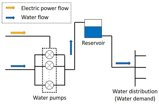
Figure 1.
Assumed water distribution system.
The water supplied from the water purification plant is pumped into the reservoir by water pumps that operate on electricity. The flow rate of the water pumps can be changed by changing power consumption using a variable speed gearbox. The water pumped into the reservoir is supplied to the water distribution network based on the water demand. This paper analyzes the provision of regulation reserves to the power system using water pumps at the pumping station. The simplified system described above is studied; a physically detailed modeling of the water distribution network is not done in this study.
2.2. Price Information
This paper assumes a scenario wherein a water pump operation plan is prepared based on the electrical energy price and the incentive price at each time slot to shift power consumption and provide regulation reserve capacity. The electrical energy price and incentive price for each time slot and the time of procuring the DR are provided by the contracted retail electricity provider or the aggregator before the preparation of the operation plan, and there is no uncertainty.
2.3. Regulation Reserves
This section discusses the assumptions about the provision and activation of regulation reserves. In this paper, the following assumptions were considered for the provision and activation of regulation reserves.
- Compensation is paid by the contractor based on the incentive price for the regulation reserve capacity provided during each time slot. In this case, the occurrence of the consideration does not depend on whether the regulation reserves are triggered during actual operation.
- In actual operation, the final volume of provision is determined through transactions with retail electricity providers and aggregators. In this paper, the amount that can be provided in the plan is treated as the amount provided.
- The time and amount of the activation of the provided regulation reserves are random.
- The imbalance from the demand plan caused by activating regulation reserves is settled between transmission and distribution companies based on the imbalanced price. The imbalance is not treated in the optimal operation planning model.
3. Optimal Operation Planning Model for Water Pumping
3.1. Power Consumption Characteristic Model of Water Pumps
This section describes a method to model the power consumption characteristics of a water pump.
First, the flow rate from the water pump is modeled. In this study, it is assumed that all water pumps are installed with the same characteristics. The total head of the water pump is given by:
where Q is the flow rate (m/h), h is the total head (m), y is the number of pumps, are the characteristic parameters of the pump, r is the pipe resistance coefficient (h/m), and H is the actual head from the pump to the reservoir (m).
Equation (1) represents the characteristic curve for the flow rate and head of the water pump. We assume that this characteristic curve is represented by a quadratic function. Equation (2) represents the characteristics of the pipe from the water pump to the reservoir.
The physical characteristics of the pump head are shown in Figure 2. The point of operation is the intersection of the characteristic curves for Equations (1) and (2), given by Points A and B in Figure 2; the flow rates from all water pumps re obtained. Thus, by using Equations (1) and (2) and solving for the flow rate Q, we can obtain the Q at the y unit operation by:
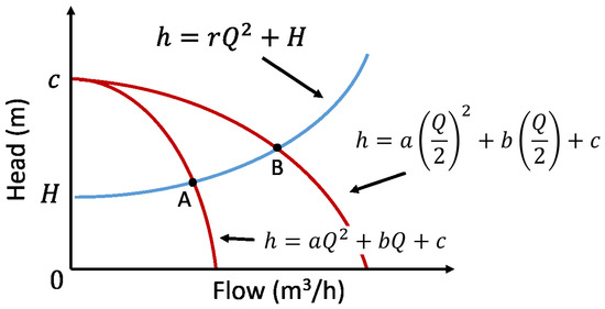
Figure 2.
Physical properties of the water pumps.
The power consumption of the water pump is modeled. The power consumption and efficiency of the water pump are given by:
where P is the power consumption (kW), is the efficiency, and are the characteristic parameters of the pump. Let the density of water be 1.0 t/m and the acceleration of gravity be 9.8 m/s. In addition, the efficiency of the water pump is approximated by a quadratic function.
The power consumption characteristics are obtained by Equation (4) when a given number of water pumps are operated. h, Q, and are a function of y, indicating that P is also a function of y.
We consider the power consumption characteristics when the rotation speed of the water pump is changed. The reference rotation speed is the rotation speed of the water pump when Equation (4) is satisfied. The relationship:
holds for the flow rate obtained by changing the rotational speed from the reference rotational speed. In Equation (6), is the flow rate from the water pump after rotation speed change (m/h), N is the reference rotation speed (rpm), and is the rotation speed (rpm) after the change.
As shown in Equation (6), the flow rate from the water pump has a proportional relationship to the ratio of rotational speed. By calculating Equations (2), (4) and (5) using the flow rate obtained by Equation (6), it is possible to obtain the power consumption of the entire water pump by varying the rotation speed of the water pump.
3.2. Approximation of the Power Consumption Characteristics of the Water Pumps
As shown in Equation (4), the power consumption characteristics of the water pump are non-linear. To formulate an optimal operational planning model for water pump as an MILP, it is necessary to linearize the non-linear power consumption characteristics.
The power consumption characteristics of the water pump and the linear approximation method are presented in Figure 3. As shown in Figure 3, the curve of the power consumption characteristics is obtained from Equation (4) for each operation of the water pumps. The number of operations with the lowest power consumption for each flow rate is the most efficient number of operations for the flow rate. The section that can be operated efficiently with an arbitrary number of pumps is considered a single pump pattern. For each pump pattern, we perform a linear approximation of the power consumption characteristics with a regression equation given by:
where are the regression coefficients.
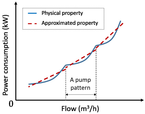
Figure 3.
Approximated properties of the water pumps.
By performing a linear regression for each pump pattern, a piecewise linear regression of the overall power consumption characteristics can be obtained.
3.3. Optimal Operational Planning Model
The proposed optimal operation planning model of the water pumps is formulated as an MILP, and it is expressed as:
subject to
where the decision variables are , power consumption (kW); , upward regulation reserve capacity (kW); , downward regulation reserve capacity (kW); , the flow rate from the water pump (m/h); , the fluctuation of the flow rate when the upward regulation reserve is provided (m/h); , the fluctuation of the flow rate when the downward regulation reserve is provided (m/h); V, the water storage in the reservoir (m); , the fluctuation in water storage caused by the activation of the regulation reserve (m); and , the indicative variable of the pump pattern (a binary variable). Other variables and constants are t, time-slot (); , time span (h); l, pump pattern (); , electrical energy price (yen/kWh); , incentive price of providing upward regulation reserve (yen/kW); , incentive price of providing the downward regulation reserve (yen/kW); , regression coefficients of the power consumption characteristics in a pump pattern l; , water demand (m/h); , upper and lower limits of the flow rate in a pump pattern l (m/h); , upper and lower limits of water storage volume in reservoirs (m); and , initial water storage volume (m).
The objective function of Equation (8) represents the net cost of operating a water supply water pump. The first term represents the cost of procuring electricity; the second and third terms represent revenues from providing regulation reserves in the increasing and decreasing demand, respectively.
Equation (9) is an equation constraint for the power consumption characteristics of a pump pattern. Equation (10) indicates the upper and lower limits on the capacity of the water pump. Equations (11) and (12) are the equation constraints on the flow rate change associated with the provision of the regulation reserves of the water pump. Equations (13) and (14) are the equation constraints on the change in water storage in the reservoir to provide regulation reserves by the water pump. Equations (15) and (16) are the upper and lower limits on the water storage capacity of the reservoir. Equation (17) is an equation constraint on the change in water storage in the reservoir between the time slots. Equations (18) and (19) represent the upper and lower limits on the regulation reserves that can be provided. Equation (20) is the initial condition for water storage in the reservoir. Equation (21) represents the termination condition for the volume of water stored in the reservoir. In this paper, the constraints are set so that water storage is equal at the beginning and end of the day. Equation (22) is the operating pattern constraint of the water pump. Any pump pattern can be selected at any time.
4. Numerical Experiment
4.1. Experimental Conditions
The parameters of the water distribution system used in the numerical experiments are listed in Table 1, and they are referenced from [21]. The profile of the water demand was set up as shown in Figure 4 based on the literature [21].

Table 1.
Parameters of the numerical experiment.
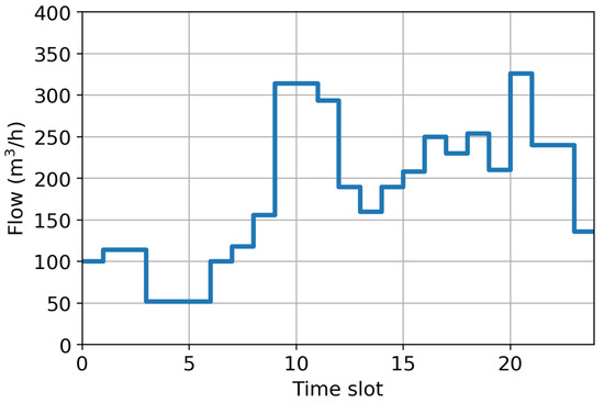
Figure 4.
Profile of hourly water demands.
The power consumption characteristics of the water pumps were calculated assuming that the flow rate can be varied up to ±40% based on the operating point of each pump number. Figure 5 shows the power consumption characteristic curves for each pump and the piecewise linear regression of the characteristic curves obtained by Equation (4) and (6). The rhombus plots represent the upper and lower limits of the flow rate and power consumption that indicate efficient operations for each pump pattern. The solid blue lines represent the power consumption characteristics; the red dotted lines represent the results of linear approximations of the power consumption characteristics for each pump pattern. The interval sandwiched by the rhombus plots is a single pump pattern, wherein one to six water pumps are operated in order from the pump pattern with the lowest power consumption. In addition, Table 2 lists the regression coefficients of the approximate straight line and the upper and lower bounds of the flow rate for each pump pattern [20].
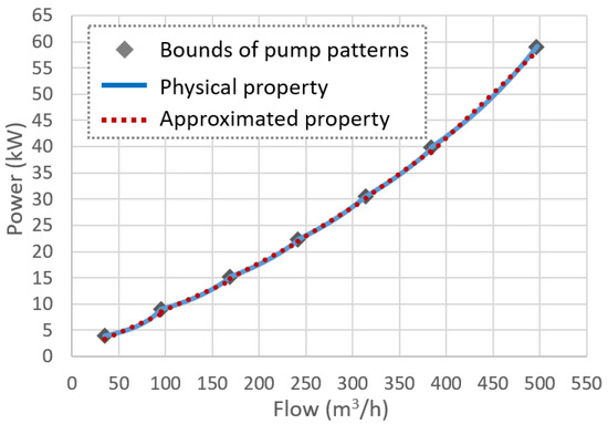
Figure 5.
Result of the approximated properties of water pumps.
Table 2.
Results of estimation parameters: Regression coefficients and higher/lower bounds of the flow rate.
To confirm the characteristics of the proposed optimal operational planning model, the optimization was performed by fixing the electrical energy price at 10 yen/kWh and using variable electrical energy prices that fluctuate according to the time of day. The optimization was performed for the case where regulation reserves were not provided and for the case where the incentive price was 20 yen/kW. Variable electrical energy prices and incentive prices of regulation reserves used in the numerical experiments are shown in Figure 6. In this figure, the blue solid line represents the electrical energy price for each time slot; the red and green bars represent the incentive price and the time slots at which regulation reserves need to be provided in an increasing or decreasing demand. Thus, the operational plans of the water pump were optimized for the following six cases.

Figure 6.
Profile of hourly variable electrical energy prices and incentive price for the provided regulation reserves.
- Case 1: The electrical energy price is fixed at 10 yen/kWh, and the price of regulation reserves is 0 yen/kW.
- Case 2: The electrical energy price is fixed at 10 yen/kWh; the price of upward regulation reserves is 20 yen/kW (); and the price of downward regulation reserves is 0 yen/kW.
- Case 3: The electrical energy price is fixed at 10 yen/kWh; the price of upward regulation reserves is 0 yen/kW; and the price of downward regulation reserves is 20 yen/kW ().
- Case 4: The electrical energy price is variable, and the price of regulation reserves is 0 yen/kW.
- Case 5: The electrical energy price is variable; the price of upward regulation reserves is 20 yen/kW (); and the price of downward regulation reserves is 0 yen/kW.
- Case 6: The electrical energy price is variable; the price of upward regulation reserves is 0 yen/kW; and the price of downward regulation reserves is 20 yen/kW ().
The optimizing solver (Gurobi Optimizer 8.1.0) was used to optimize the optimal operational planning model.
4.2. Results
4.2.1. In the Case of Fixed Electrical Energy Prices
The power consumption and regulation reserves to be provided for the operational plan of the water pump obtained in Cases 1 to 3 are shown in Figure 7. The solid red, dashed blue, and dashed green lines indicate the planned power consumption of the water pump, when upward regulation reserve capacity provided to the power system is fully activated, and when downward regulation reserve capacity provided to the power system is fully activated, respectively.
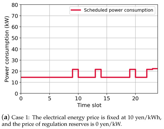
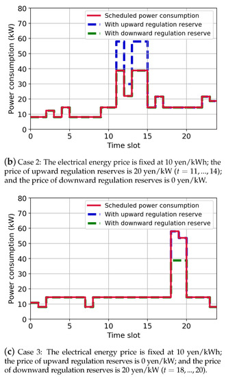
Figure 7.
Results for the electrical power consumption of water pumps under the fixed electrical energy price. The solid red, dashed blue, and dashed green lines indicate the planned power consumption of the water pump, when upward regulation reserve capacity provided to the power system is fully activated and when downward regulation reserve capacity provided to the power system is fully activated, respectively.
The case that does not provide the regulation reserves as shown in Figure 7a (Case 1) is equivalent to the problem of minimizing the daily power consumption of the water pumps. Therefore, it can be confirmed that the system operates while reducing the number of water pumps that need to be started. In the case of the provision of regulation reserves (Cases 2 and 3), the operational plan is such that the income from the provision of regulation reserves is maximized.
In Case 2, where the provision of the upward regulation reserves is required, as shown in Figure 7b, the operation is conducted such that the number of starting water pumps is increased during the required time slots (–14) to ensure upward regulation reserves. The pump pattern that operates six water pumps has a larger capacity to provide regulation reserves compared to the other pump patterns, and therefore, there are time slots when the number of pumps in operation is increased to maximize the income by providing regulation reserves. In Case 3, where the provision of downward regulation reserves is required, as shown in Figure 7c, six water pumps were operated during a part of the required time slots () to secure the downward regulation reserve capacity.
The change in the water storage volume in the reservoir during planning and activating regulation reserves is shown in Figure 8. The solid red line shows the planned water storage volume of the reservoir. The blue and green dashed lines show the change in water storage volume when the provided regulation reserves are activated. The yellow dotted line represents a changed scenario in the water storage volume when the provided regulation reserves are activated for only half the time in each time slot. The scenario for activating regulation reserves is the same as that assumed in [20].
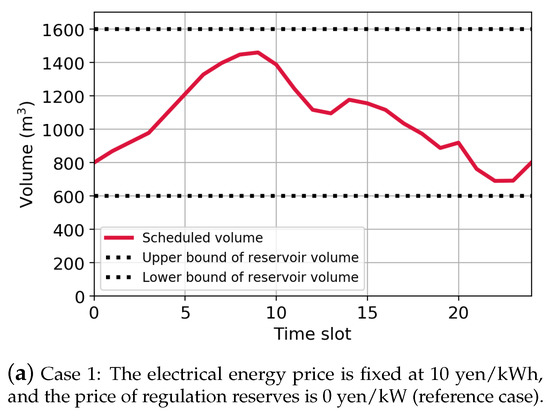
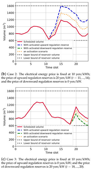
Figure 8.
Results for the volume of the reservoir under the fixed electrical energy price. The solid red line shows the planned water storage volume of the reservoir. The blue and green dashed lines show the change in water storage volume when the provided regulation reserve capacities are fully activated. The yellow dotted line represents a changed scenario in the water storage volume when the provided regulation reserves are activated for only half the time in each time slot.
Other cases are discussed using the case shown in Figure 8a as a reference case. As shown in Figure 8b, Case 2 provides upward regulation reserves. The water storage volume when the provided regulation reserves are activated is higher than the planned water storage volume. Further, the planned water storage volume in the reservoir in the first half time slots remained lower than that in Case 1. As shown in Figure 8c, since Case 3 provides the downward regulation reserves, the water storage volume when the provided regulation reserves are activated is lower than the planned water storage volume. As in Case 2, the planned water storage volume in the reservoir remained lower than that in Case 1. This is achieved by the fact that, as shown in Figure 7c, six pumps are being operated to maximize the provided amount of downward regulation reserves.
As described above, in Cases 1 to 3—where the electrical energy price was fixed at 10 yen/kWh—an operational plan that secured a profit by providing regulation reserves while reducing the power consumption of the water pumps was employed. In addition, a robust operational plan for the activation of regulation reserves was obtained that would satisfy the constraints of the reservoir capacity even if all the provided regulation reserves were activated.
4.2.2. Variable Electrical Energy Price
The optimization results when the electrical energy price varies over time are as shown in Figure 6. The power consumption and regulation reserves provided in the operational plan of the water pumps obtained in each case are shown in Figure 9. The transition of water storage volume in the reservoir is shown in Figure 10 when the operational plan is implemented.
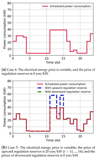
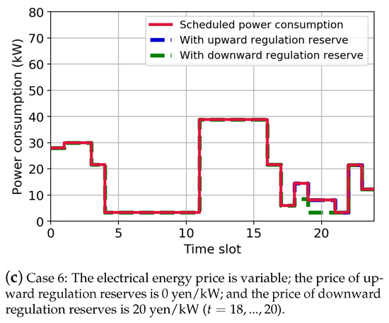
Figure 9.
Results for the electrical load of water pumps under the variable electrical energy prices. The solid red, dashed blue, and dashed green lines indicate the planned power consumption of the water pump, when upward regulation reserve capacity provided to the power system is fully activated and when downward regulation reserve capacity provided to the power system is fully activated, respectively
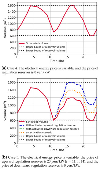
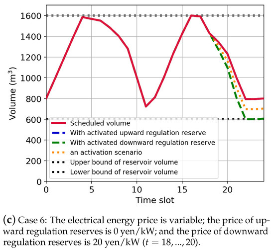
Figure 10.
Results for the volume of the reservoir under the variable electrical energy prices. The blue and green dashed lines show the change in water storage volume when the provided regulation reserve capacities are fully activated. The yellow dotted line represents a changed scenario in the water storage volume when the provided regulation reserves are activated for only half the time in each time slot.
For Case 4, the regulation reserves are not provided as shown in Figure 9a; compared to that in Figure 7a, the operation that concentrates the pump operation in the time slots when the electrical energy price is low was obtained. For Case 5, the provision of the upward regulation reserve is required, as shown in Figure 9b; compared to Figure 7b, the power consumption of the water pumps in the time slots when the electrical energy price is high decreases and shifts to the time slots before and after. For Case 6, downward regulation reserves are required as shown in Figure 9c; compared to Figure 7c, the power consumption of the water pumps in the time slots when the electrical energy price is high decreases and shifts to the time period before and after. In addition, the power consumption of 18–20 is increased and the power consumption of the time slots before and after is decreased when compared to Figure 9a. This is attributed to the operation of the maximum power in each pump pattern to ensure sufficient capacity to provide the downward regulation reserve capacity.
The transition of water storage volume in the reservoir of planning and activating regulation reserves is shown in Figure 10. As shown in Figure 10b, Case 5 provides the upward regulation reserves, and therefore, the water storage volume when the provided regulation reserves were activated was higher than the planned volume. As shown in Figure 10c, because Case 6 provided downward regulation reserves, the water storage volume when the provided regulation reserves were activated was lower than the planned volume. In addition, compared to Case 4, the operation of increasing the water storage volume in the reservoir to 18–20 is obtained to save the lower capacity of the reservoir when the downward regulation capacity is provided.
In Cases 4 to 6 with variable electrical energy prices, an operation plan that avoids operating the water pumps when the electrical energy price is higher and operates them at less expensive times can be obtained. In addition, a robust operational plan to activate the regulation reserves was obtained that would satisfy the constraints of reservoir capacity even if all the regulation reserves were activated.
4.2.3. Comparison of Operational Costs
We compare the objective function values of the optimal operational planning models obtained in Cases 1 to 6, i.e., the net operational costs. Table 3 shows the operational costs obtained in each case.
Table 3.
Results of the objective function value.
We compare the operational costs, which are the objective function values obtained in each case. We consider Case 1, which is the objective function value when power consumption is minimized, as a criterion. In Case 2, the operating cost was reduced by 30.0%, and in Case 3, it was reduced by 11.7%. The difference in the reduction rate between Cases 2 and 3 is attributed to the water demand profile assumed in this study and the constraints on water storage volume (termination condition and lower limit of water storage). In Case 5, the operating cost was reduced by 36.0%, and in Case 6, it was reduced by 4.5%. The reduction in the operating cost in Case 5 was relatively greater than that in the other cases. This is because the revenue obtained by the provision of regulation reserves increased because of an operational plan in which six units, by which a relatively large amount of regulation reserves could be provided, was operated.
Thus, the DR using the water pumps can reduce the net operating cost of the water pumps’ operation by providing regulation reserves to the power systems and receiving income based on incentive prices.
5. Conclusions
In this paper, an optimal operation planning model for water pumps in a water distribution system was proposed; this model can shift the electricity demand based on the electrical energy price and provide regulation reserves to the power system. The specific results are listed below.
- For the optimal operation planning problem of the water pumps that provides regulation reserves, a method to ensure that the water storage volume in the reservoir is within the constraints and to maintain a stable water distribution under the uncertainty of the activation of the provided regulation reserves was proposed.
- Based on electrical energy and incentive prices for the provision of regulation reserves, a model was proposed that allows drawing an operation plan for water pumps that minimizes the net energy cost.
- As a case study, a numerical experiment was conducted on changing the electrical energy and incentive prices. The results confirmed the time shift in power consumption with the electrical energy price as a control signal. To maximize the revenues from the provision of regulation reserves, an operational plan was obtained that adjusts the planned water storage volume for the time slots when regulation reserves were required.
- Through a comparison of the objective function values obtained as a result of the numerical experiments, a net operating cost reduction in water pump operation was achieved by establishing a new source of income: the use of water pumps to provide regulation reserves to the power system.
The results of this study indicate that the pumping operation of the water distribution system can be controlled by electric energy prices and incentive prices. In the future, it is expected that the water distribution system can be integrated with the power system to reduce the cost of energy supply for the whole society and to use the VRE effectively.
In this study, a simplified water distribution system was modeled. In order to incorporate the model into the actual water supply system, it is necessary to expand the model to be able to calculate more detailed geophysical quantities, including pipe network analysis.
Author Contributions
S.N. conceived of and designed the research methodology and analyzed and drafted this manuscript. T.I. supervised the research and provided suggestions regarding the research. Both authors have read and agreed to the published version of the manuscript.
Funding
This study was supported by the Ministry of the Environment (MOE), Japan, “Contracted work of survey on New Systems for Low Carbon Power Generation” in 2020.
Conflicts of Interest
The authors declare no conflict of interest.
References
- Water Supply Division, Health Bureau, Ministry of Health, Labour and Welfare. Guide to Environmental Measures in Water Supply Projects (Revised Edition). 2009. Available online: https://www.mhlw.go.jp/za/0723/c02/c02-02.html (accessed on 15 April 2019).
- Health Bureau, Ministry of Health, Labour and Welfare. New Water Supply Vision. 2013. Available online: https://www.mhlw.go.jp/seisakunitsuite/bunya/topics/bukyoku/kenkou/suido/newvision/1_0_suidou_newvision.htm (accessed on 15 April 2019).
- American Water Works Association. Computer Modeling of Water Distribution Systems: AWWA Manual of Water Supply Practice, 3rd ed.; American Water Works Association: Denver, CO, USA, 2012. [Google Scholar]
- Arai, Y.; Horie, T.; Koizumi, A.; Inakazu, T.; Masuko, A.; Tamura, S.; Yamamoto, T. Minimizing Power Usage in Water Distribution System Using Mixed Integer Linear Programming. J. Jpn. Soc. Civ. Eng. Ser. G 2012, 68, II273–II281. (In Japanese) [Google Scholar]
- Takahashi, S.; Koibuchi, H.; Adachi, S.; Takemoto, T.; Koizumi, K. Pump Operation Scheduling for Power Demand Response in Water Transmission Systems. IEEJ Trans. EIS 2016, 136, 1200–1208. (In Japanese) [Google Scholar] [CrossRef]
- Chang, Y.; Choi, G.; Kim, J.; Byeon, S. Energy Cost Optimization for Water Distribution Networks Using Demand Pattern and Storage Facilities. Sustainability 2018, 10, 1118. [Google Scholar] [CrossRef]
- Afshar, A.; Massoumi, F.; Afshar, A.; Marino, M.A. State of the art review of ant colony optimization applications in water resource management. Water Resour. Manag. 2015, 29, 3891–3904. [Google Scholar] [CrossRef]
- Luna, T.; Ribau, J.; Figueiredo, D.; Alves, R. Improving energy efficiency in water supply systems with pump scheduling optimization. J. Clean. Prod. 2019, 213, 342–356. [Google Scholar] [CrossRef]
- Gleixner, A.; Held, H.; Huang, W.; Vigerske, S. Towards globally optimal operation of water supply networks. Numer. Algebr. Control Optim. 2012, 2, 695–711. [Google Scholar] [CrossRef]
- Burgschweiger, J.; Gnadig, B.; Steinbach, M.C. Optimization models for operative planning in drinking water networks. Optim. Eng. 2008, 10, 43–73. [Google Scholar] [CrossRef]
- Menke, R.; Abraham, E.; Parpas, P.; Stoianov, I. Demonstrating demand response from water distribution system through pump scheduling. Appl. Eng. 2016, 170, 377–387. [Google Scholar] [CrossRef]
- Hirano, T.; Ashida, Y.; Lu, Y.; Izukura, S.; Nishioka, I.; Fujimaki, R. Stable and Energy Efficient Operation in a Large-scale Water Distribution Network. IPSJ Trans. Math. Model. Appl. 2017, 10, 33–42. [Google Scholar]
- Zimmermann, B.; Gardian, H.; Rohrig, K. Cost-Optimal Flexibilization of Drinking Water Pumping and Treatment Plants. Water 2018, 10, 857. [Google Scholar] [CrossRef]
- Fooladivanda, D.; Taylor, J.A. Energy-Optimal Pump Scheduling and Water Flow. IEEE Trans. Control Netw. Syst. 2018, 5, 1016–1026. [Google Scholar] [CrossRef]
- Fracasso, P.T.; Barnes, F.S.; Costa, A.H.R. Energy Cost Optimization in Water Distribution Systems using Markov Decision Processes. In Proceedings of the 2013 International Green Computing Conference, Arlington, VA, USA, 27–29 June 2013; pp. 1–6. [Google Scholar]
- EPANET. Available online: https://www.epa.gov/water-research/epanet (accessed on 20 April 2020).
- GUROBI Optimizer. Available online: https://www.gurobi.com/ (accessed on 6 March 2020).
- CPLEX. Available online: https://www.ibm.com/jp-ja/analytics/cplex-optimizer (accessed on 6 March 2020).
- Takahashi, M. Study on Possibility of Fast Demand Response Mitigating Grid Balancing Challenges in Japanese Power System with Large-scale Renewable Energy Integration. CRIEPI Res. Rep. 2016, Y13030, 16–18. (In Japanese) [Google Scholar]
- Negishi, S.; Ikegami, T. A Water Pumping Scheduling Method in Water Distribution System with Providing Balancing Reserves to Power System. IEEJ Trans. Power Energy 2019, 139, 757–766. (In Japanese) [Google Scholar] [CrossRef]
- Investigating R&D Committee on New Development of Computational Intelligence Techniques and Their Applications to Industrial Systems. Optimization Benchmark Problems for Industrial Applications. IEEJ Tech. Rep. 2013, 1287, 13–17. (In Japanese) [Google Scholar]


Publisher’s Note: MDPI stays neutral with regard to jurisdictional claims in published maps and institutional affiliations. |
© 2021 by the authors. Licensee MDPI, Basel, Switzerland. This article is an open access article distributed under the terms and conditions of the Creative Commons Attribution (CC BY) license (http://creativecommons.org/licenses/by/4.0/).