Performance Enhancement of a Partially Shaded Photovoltaic Array by Optimal Reconfiguration and Current Injection Schemes

Abstract

The output of a photovoltaic array is reduced considerably when PV panels are shaded even partially. The impact of shading causes an appreciable loss in power delivery, since the PV panels are connected in series and parallel to contribute to the required voltage and power for the load. The prevailing research on mitigating the shading impact is mostly based on complex reconfiguration strategies where the PV panels are subjected to complex rewiring schemes. On the other hand, to disperse the shading many studies in the literature defend the physical rearrangement of the panels. The available intensive reconfiguration schemes, such as the series parallel (SP), bridge link (BL), honeycomb (HC), and total cross tied (TCT) schemes, try only to mitigate the shading impact and there is no scope for compensation; as a result, a loss of output power is inevitable. In the proposed research work, both the mitigation of and the compensation for the losses incurred due to shading are studied. In this work, an optimal reconfiguration scheme is adopted to reduce the shading impact and a power electronic circuit with a battery source is designed to compensate for the shading losses in all aspects. In the optimal reconfiguration scheme, a bifurcation strategy is adopted in each column and the electrical connections of the PV panels are interchanged such that the shading impact is dispersed. The power electronic circuit consists of a half-bridge buck converter with a battery source that injects the current required by a shaded column. This setup compensates for the shaded PV array’s power and improves the efficiency of the total system. The proposed scheme was implemented in a 3200 W system and subjected to various shading patterns, including single panel shading, corner shading, long and wide shading, and random shading. The proposed scheme was simulated in the MATLAB Simulink environment and compared with static 4 × 4 PV array configurations, including the series parallel (SP), bridge link (BL), honeycomb (HC), and total cross tied (TCT) configurations. The comparative performance was assessed in terms of mismatch power loss, fill factor, and efficiency. The proposed system is suitable for all shading patterns and was proved to be very efficient even in the worst shading, where 1353 W was saved.

1. Introduction

The solar photovoltaic (PV) system is a prominent power source among all the renewable energy sources available due to its unique features of being scalable and portable. One of the major challenges that PV power sources inherently have is the existence of nonlinear current–voltage (I-V) and power–voltage (P-V) characteristics with respect to irradiation and temperature [1]. The nonlinear I-V and P-V curves will have a single peak power point at which the PV panel is capable of delivering the maximum power at a given time. This mechanism of tracking power is called the maximum power point tracking (MPPT) scheme [2,3]. Partial shading (PS) is a phenomenon that happens when a part of the PV panel is shaded by any hindrance, such as the branch of a tree, a pole, a cloud, birds’ poop, etc. Due to PS, the output power–voltage (P-V) curves become more complex as there will be several power peaks rather than a single power peak. The well-ingrained MPPT techniques, such as perturb and observe (P&O) and incremental conductance (INC), may fail miserably as they get stuck at the local maximum power point (LMPP) and do not extract the global maximum power point (GMPP) [4,5,6]. In order to overcome the local MPPs and grasp the global MPP, soft computing MPPT algorithms have been proposed. The most commonly used soft computing MPPT techniques are particle swarm optimization (PSO), differential evolution (DE), ant colony optimization (ACO), and the shuffled frog leap algorithm (SFLA) [7,8,9,10,11,12]. On the other hand, soft computing MPPT techniques are difficult to deploy under practical environmental conditions as the coding complexity and the embedded processor’s deployment are major hurdles [13,14,15]. Therefore, research on dispersing the shading impact through reconfiguring the PV panels seems to be the pragmatic solution to mitigate the shading impact and to render a P-V curve without multiple power peaks [16].

Employing bypass diodes in parallel to the PV panels inherently reduces the shading impact but the major drawback is that, even if a fraction of the panel is shaded, the particular panel will be discarded from the cumulative PV array, which decreases the power efficiency [17,18,19]. Additionally, the employment of flyback diodes results in multiple power peaks in P-V curves. Reconfiguration of PV panels is a prudent approach to the mitigation of the shading impact. By rearranging the panels, the row current can be made equal. The standard configuration schemes are the series parallel (SP), bridge link (BL), honeycomb (HC), and total cross tied (TCT) schemes. The various configuration patterns are shown in Figure 1. The choice of configuration is made based upon the load requirements and other constraints. Of the abovementioned reconfiguration schemes, the TCT configuration renders more output than the other configurations [19]. The major drawback of the TCT configuration is the requirement of more wire connections. Therefore, the quest to find a new, optimum reconfiguration scheme in this research area has been persistent.

The research work carried out on reconfiguration may be categorized as: (i) relocation of PV panels; (ii) rewiring of PV panels; or (iii) PV array reconfiguration. The sudoku scheme and zigzag method demonstrated improved power delivery of the PV system during shading [20]. The biggest challenge of this scheme is the involvement of manpower or the need to physically displace the panels. The arrangement as well as the process involved is cumbersome [20].

The rewiring concept, on the other hand, requires a complex wiring arrangement, a huge number of sensors, and switch requirements. With the advent of high-end processors, low-power-consumption devices, and fast switching times, electrical array reconfiguration (EAR) schemes have become more reliable over time. Matrix algorithms and combinational switching schemes were proposed, but they have not become prominent candidates due to their complex switching pattern. Therefore, although many reconfiguration schemes have been proposed in this research area, a pragmatic solution is still not readily available. The S-P reconfiguration scheme is used in most practical applications [21]. This scheme is very compatible with the plug-and-play alignment, and the scope for modification is very broad. Most research papers that defend the TCT scheme claim that it is a preferable method, but it currently cannot be used for PV arrays with complex shading [22]. This research work proposes and develops two solutions for mismatch and shading losses in a SP-connected PV array. The first solution is a panel swapping algorithm that swaps between the healthy and unhealthy panels in a row, thereby dispersing the shading. Alkatani et al. [23] and Bendary et al. [24] performed interesting work on repositioning the panels that caters to aging factor issues and fault clearing, respectively, to enhance the power output; however, the authors did not consider the shading constraint. The second novel solution is injecting the current required by the row to avoid the mismatch losses. The current is fed through a half-bridge converter with a buck converter circuit sourced by a low-voltage battery. Winston et al. [25] proposed a current compensation scheme, but it also requires the employment of the TCT and BL configurations, which in turn increases the system’s complexity. Moreover, only a simple TCT topology was considered in the work. Again, if a large number of panels are shaded within a short span of time, no prudent solution is possible. This work proposes novel schemes to address the shading impact with a worst-case analysis.

This paper is organized as follows. The impact of partial shading and the details of the proposed reconfiguration and current injection schemes are presented in Section 2 and Section 3, respectively. Section 4 presents the simulation results. The conclusions drawn from this study are provided in Section 5.

2. PV Model and Impact of Partial Shading

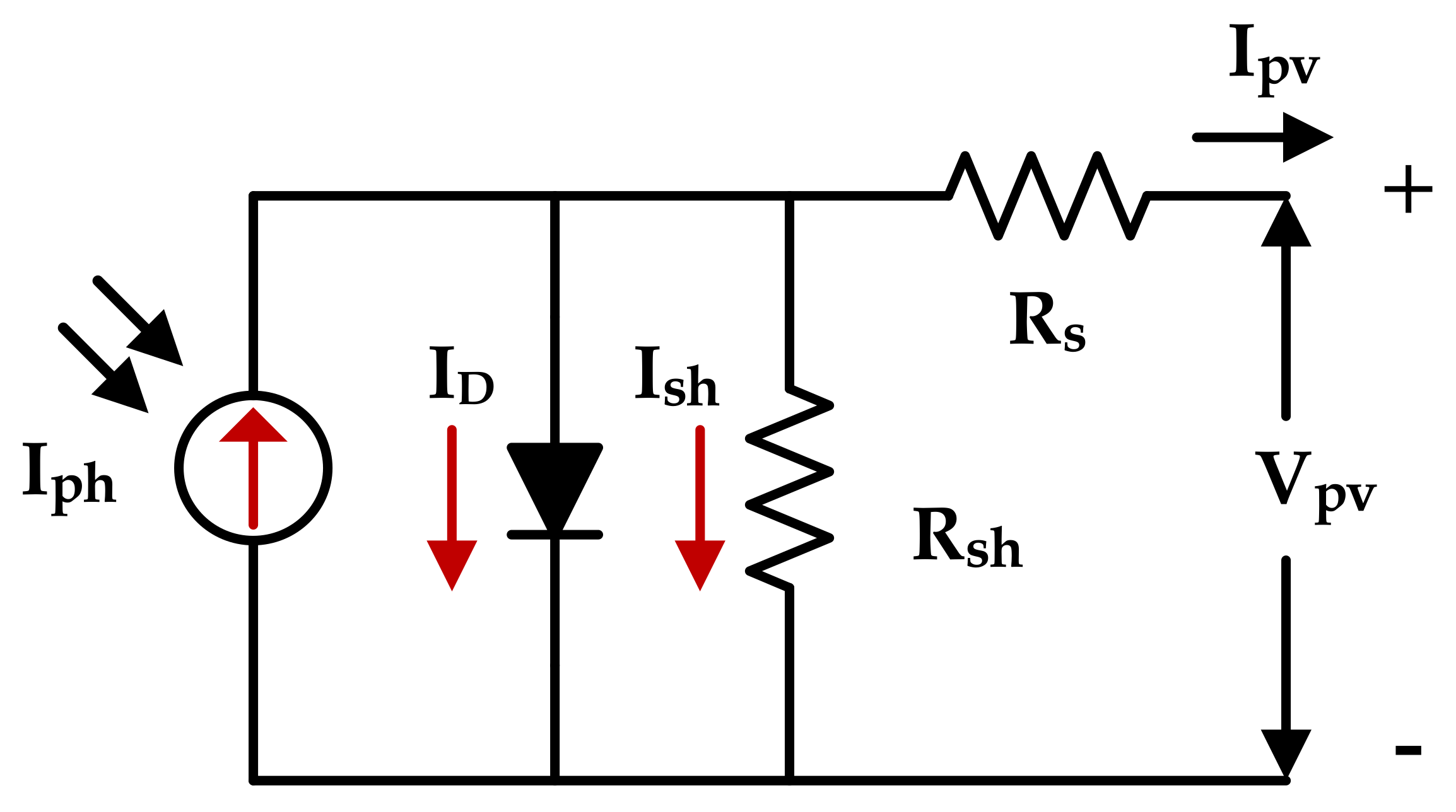
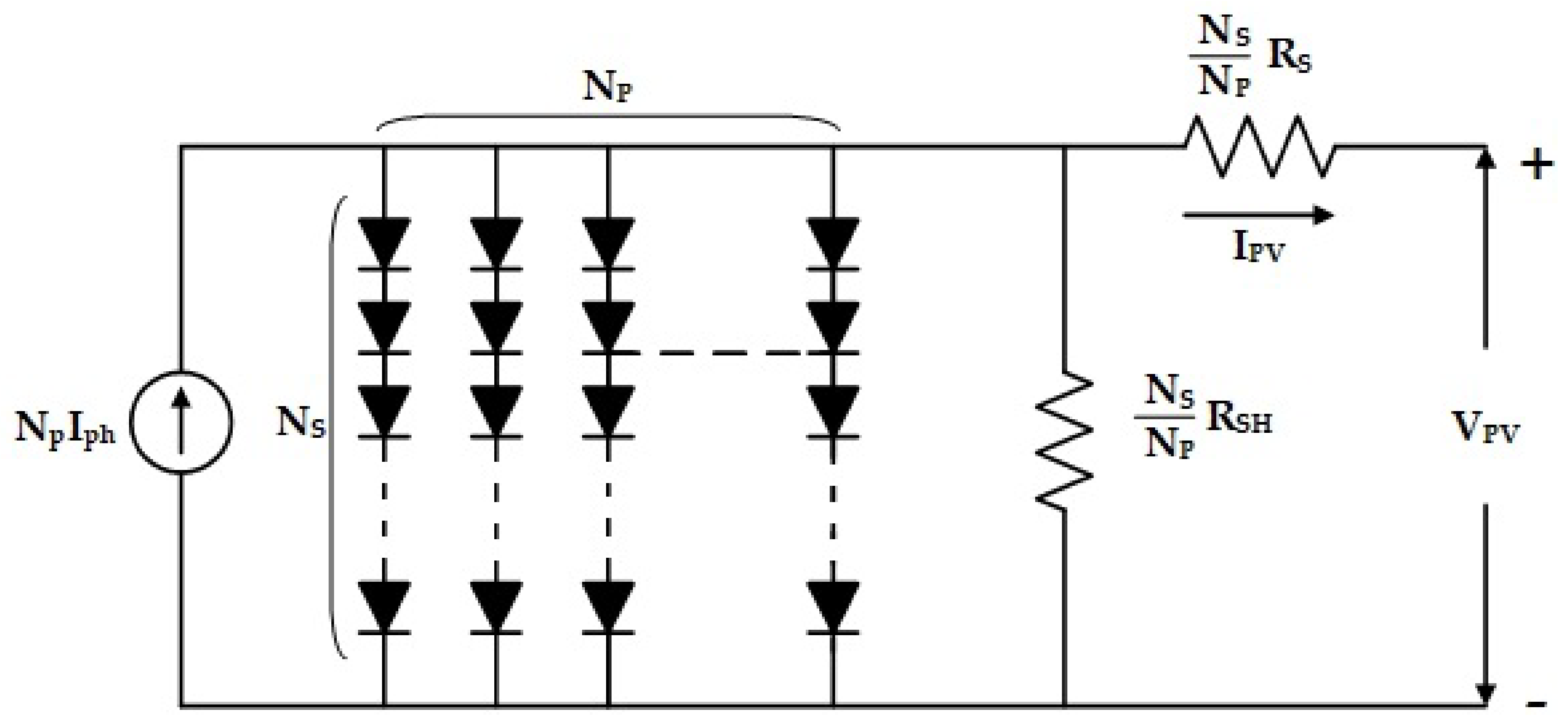
In this section, the PV model and partial shading and its effects are discussed. Appropriate modeling of a typical PV cell, the functional unit of a PV panel, has to be carried out scrupulously. In addition, an analysis of the impacts of partial shading on a given PV system is essential to draw conclusions based on the choice of solutions to mitigate it.

2.1. PV Model

Because of its simple structure, the single-diode PV model was used in this study. The single-diode PV model happened to be the most viable one due to the involvement of the minimum number of parameters [26]. Figure 2 shows an equivalent circuit of the single-diode PV cell. The equivalent model has a current source (I_ph), a diode in anti-parallel, series resistance (R_s), and parallel resistance (R_sh).

The output current from the PV cell (I_PV) is obtained through Kirchhoff’s current law, which is given below

$${\mathrm{I}}_{\mathrm{PV}}={\mathrm{I}}_{\mathrm{ph}}-{\mathrm{I}}_{\mathrm{D}}-{\mathrm{I}}_{\mathrm{sh}}$$

(1)

where the photo-current generated by the incident irradiation is given by I_ph, the nonlinearity of the diode is given by I_D, and the current flowing through the shunt resistor is given by I_sh.

Substituting I_D and I_sh in Equation (1), I_PV is given in Equation (2)

$${\mathrm{I}}_{\mathrm{PV}}={\mathrm{I}}_{\mathrm{ph}}-{\mathrm{I}}_{\mathrm{O}}\left\{\exp \left[\frac{\left({\mathrm{V}}_{\mathrm{PV}}+{\mathrm{I}}_{\mathrm{PV}}{\ast \mathrm{R}}_{\mathrm{s}}\right)}{{\mathrm{N}}_{\mathrm{s}}\ast \left(\frac{{\mathsf{\eta }\mathrm{k}}_{\mathrm{b}}\mathrm{T}}{\mathrm{q}}\right)}\right]-1\right\}-\frac{{\mathrm{V}}_{\mathrm{PV}}+{\mathrm{I}}_{\mathrm{PV}}{\ast \mathrm{R}}_{\mathrm{s}}}{{\mathrm{R}}_{\mathrm{sh}}}$$

(2)

where I_O is the saturation current of the diode, $\mathsf{\eta }$ is the ideality constant, q is the electron charge (1.602 × 10⁻¹⁹C), k is the Boltzmann constant (1.3806503 × 10⁻²³J/K), T is the cell temperature, and V_PV is the voltage generated by the PV cell for the irradiation.

A PV array is developed by employing series-connected modules (N_S) and parallel-connected modules (N_P) as shown in Figure 3.

Now, I_PV is shown in terms of the PV array in Equation (3).

$${\mathrm{I}}_{\mathrm{PV}}={\mathrm{N}}_{\mathrm{p}}{\mathrm{I}}_{\mathrm{ph}}-{\mathrm{I}}_{\mathrm{O}}\left\{\exp \left[\frac{\left({\mathrm{V}}_{\mathrm{PV}}+{\mathrm{I}}_{\mathrm{PV}}{\ast \mathrm{R}}_{\mathrm{s}}\frac{{\mathrm{N}}_{\mathrm{s}}}{{\mathrm{N}}_{\mathrm{p}}}\right)}{{\mathrm{N}}_{\mathrm{s}}\ast \left(\frac{{\mathsf{\eta }\mathrm{k}}_{\mathrm{b}}\mathrm{T}}{\mathrm{q}}\right)}\right]-1\right\}-\frac{{\mathrm{V}}_{\mathrm{PV}}+{\mathrm{I}}_{\mathrm{PV}}{\ast \mathrm{R}}_{\mathrm{s}}\frac{{\mathrm{N}}_{\mathrm{s}}}{{\mathrm{N}}_{\mathrm{p}}}}{\frac{{\mathrm{N}}_{\mathrm{s}}}{{\mathrm{N}}_{\mathrm{p}}}{\mathrm{R}}_{\mathrm{sh}}}$$

(3)

Table 1. Specifications for a KyoceraKC200GT 200 W panel (electrical performance under Standard Test Conditions (STCs)).

Specification Parameters	Values
Maximum Power (Pmax)	200.143 W
Maximum Power Voltage (Vmp)	26.3 V
Maximum Power Current (Imp)	7.61 A
Open Circuit Voltage (Voc)	32.9 V
Short Circuit Current (Isc)	8.21 A
Temperature Coefficient of Voc	−0.1230 V/K
Temperature Coefficient of Isc	0.0032 A/K
Number of Series-Connected Cells in the Module	54

presents the specifications of the PV module under standard test conditions (STCs) at 1000 W/m² and 25 ^oC.

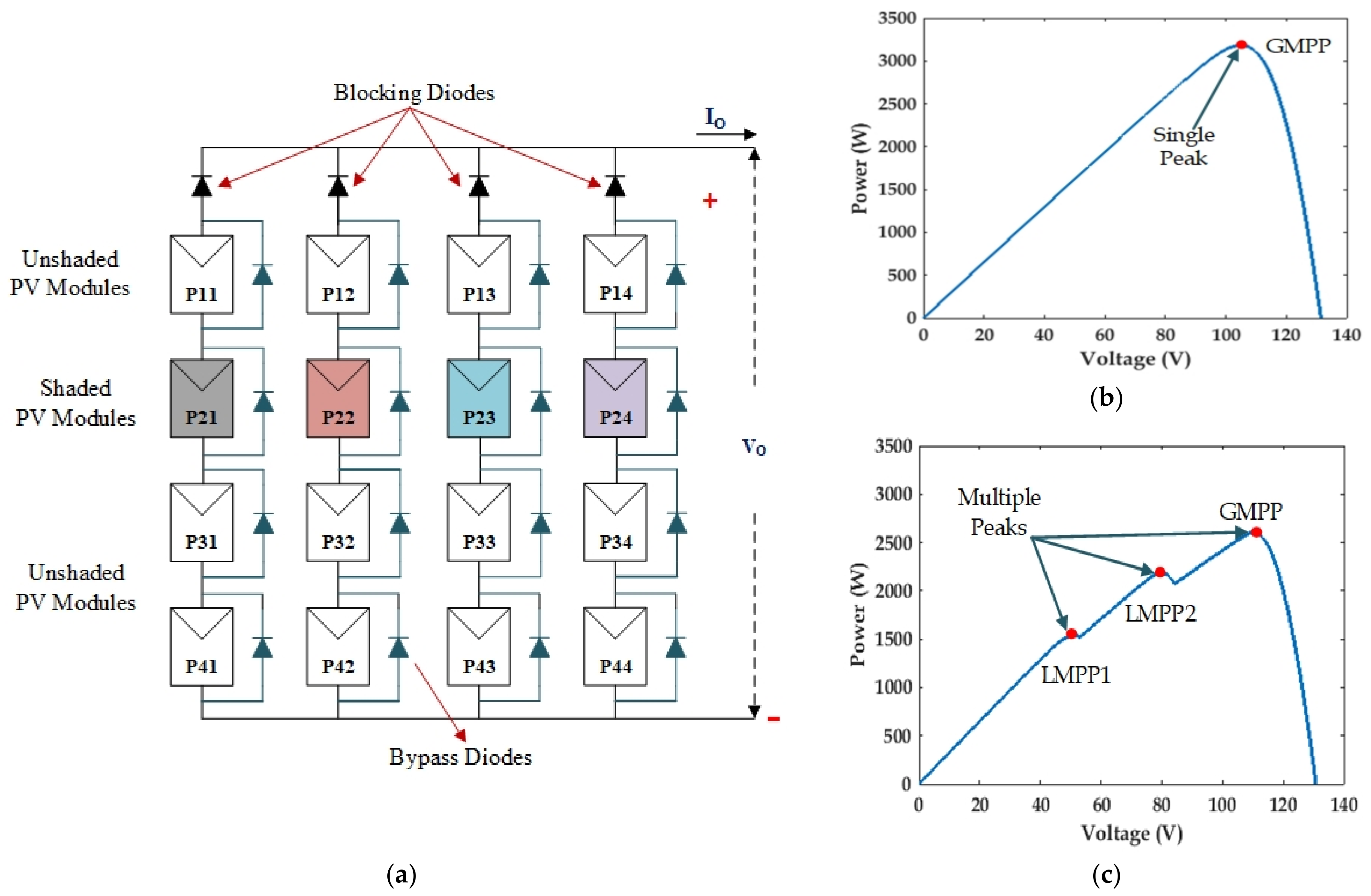
2.2. Partial Shading and Its Effects

The performance of solar panels is satisfactory when they are exposed to homogenous irradiation. During partial shading, the panels that are shaded will act like a load and, therefore, the net power generation will fall substantially. From this perspective, some panels of the array that are shaded will become overheated compared with the other healthier panels. This heating impact may cause damage (hotspots) to the PV array. To avoid this issue, flyback or bypass diodes are connected across the PV panels that relieve the shaded panel from the heat and reverse the voltage impacts. The partial shading condition of the PV array and its characteristics are shown in Figure 4.

The PV curve will vary dynamically with respect to the irradiation. There will be a peak power point on each curve. Therefore, it is imperative that the PV panels operate at their peak power for the given environmental conditions. When shading occurs, the irradiation of each panel varies, and the voltage and current values also vary. Due to this, the cumulative power–voltage (P-V) curves will have multiple bumps in them. The MPPT algorithms during partial shading may get stuck at the local maximum and will not grasp the global peak power. In Figure 4b, there are three power peaks: one global power peak at 2500 W, a second peak at 2100 W, and a third one at 1500 W. Among these peak power points, the global maximum is at 2500 W and the local minimum is at 1500 W. Therefore, the impact of partial shading is not only the reduction in power generated but also making the MPPT ineffective by grasping the local maxima. A prudent scheme is needed to enhance the power delivery during partial shading and also to make the P-V curve unimodal, which in turn will allow the MPPT techniques to grasp the peak power.

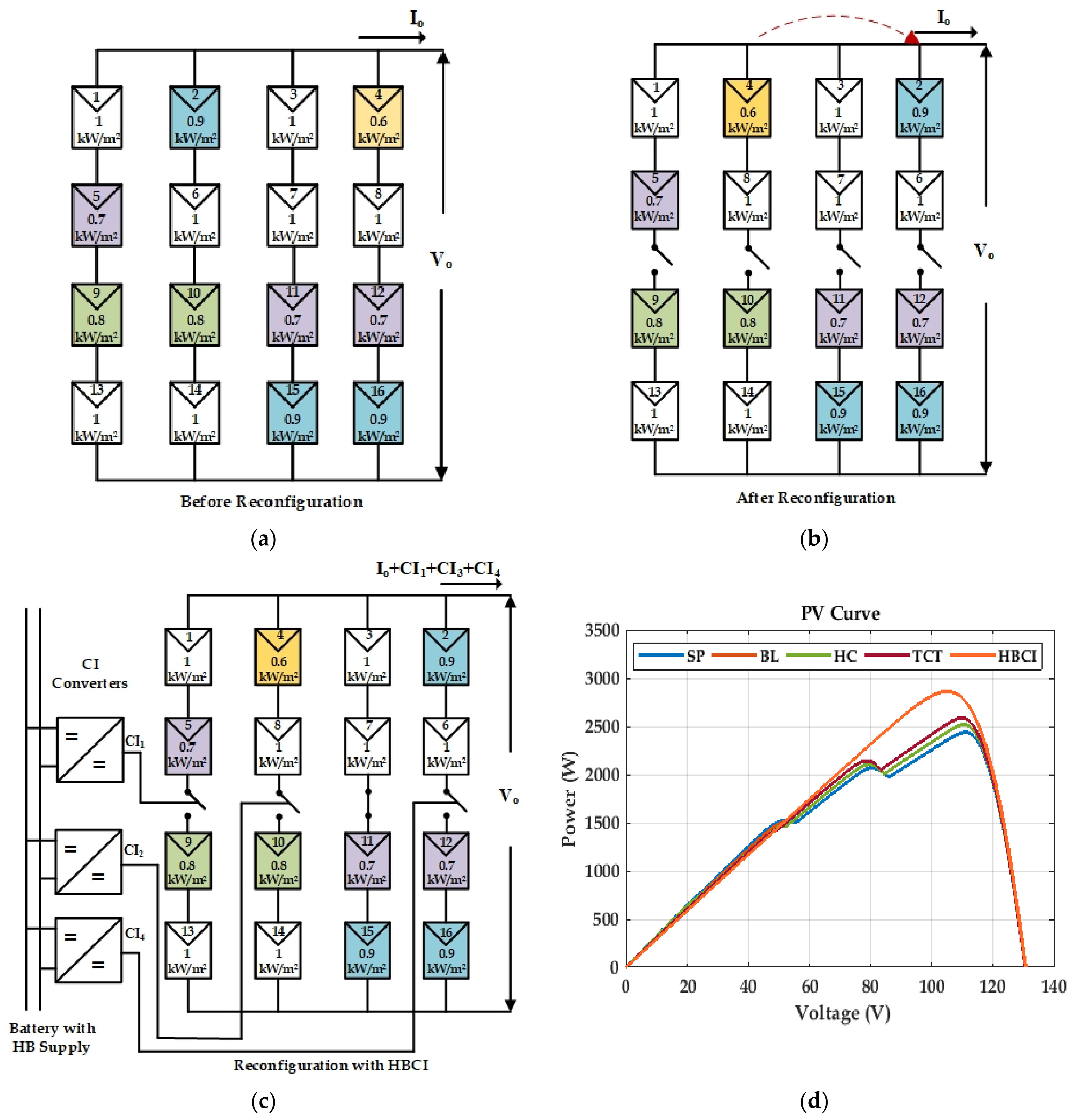
3. Optimal Reconfiguration and Proposed Half-Bridge Current Injection Scheme

Due to the uneven shading, the PV array exhibits multiple output power peaks that, in turn, make the tracking scheme cumbersome. In this research work, a power electronic circuit-aided current injection scheme is proposed. To make the current injection scheme a versatile one, an optimal dynamic reconfiguration scheme also adopted based on the irradiation equalization method, which facilitates the dispersion of the shading and thereby makes the profile of the P-V curve have one peak power point. The current injection technique is proposed to compensate for the power lost due to the shading. The compensation scheme possesses a half-bridge flyback converter, a buck converter, and a battery source as its components. The optimal reconfiguration method and the proposed half-bridge current injection method are shown in Figure 5.

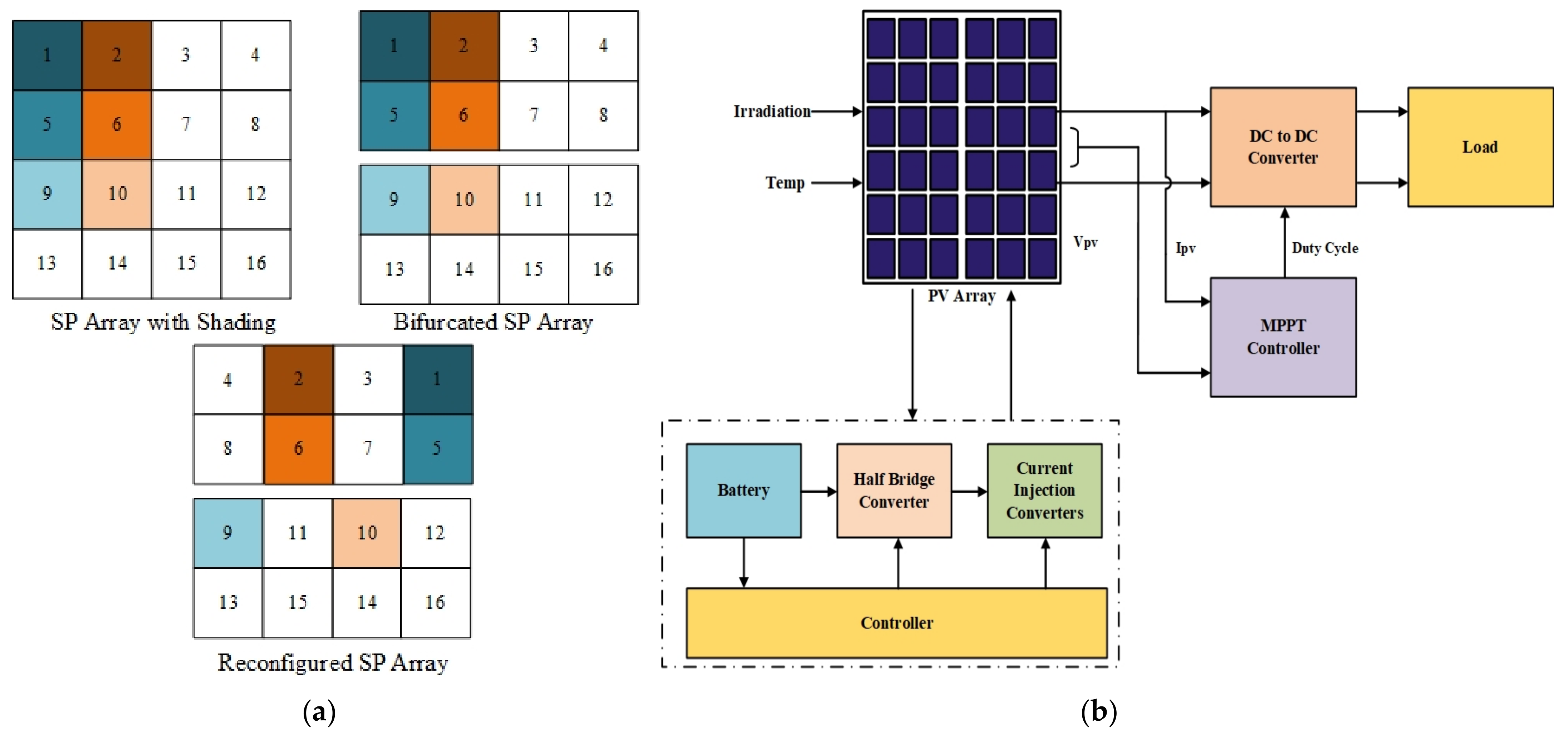
3.1. Optimal Reconfiguration

The reconfiguration scheme is based on the irradiation equalization method. This equalization scheme cannot be a complete solution to partial shading since the emergence of multiple power peaks in a severely shaded PV array even after reconfiguration is inevitable. This leads to a loss of active output power. The reconfiguration technique reduces the shading impact but cannot make up for the power lost due to shading.

The proposed optimal reconfiguration scheme is presented in Figure 5a. Here, a 4 × 4 SP array was considered, and a switching matrix-based reconfiguration method was deployed to ensure that an equal amount of current was flowing through each column of the array. As illustrated in Figure 5a, each string was divided into two parts and the whole array was divided into eight parts. Switching matrix control signals were fed to the switches in the PV array.

When partial shading occurs, the controller receives a mismatching current and voltage from the given series parallel (SP) PV array. The controller will identify the possible configuration combinations and swap the connections of the PV modules in such a way that all column currents are equal. Since the column currents are the same, the P-V curve will have a smooth single peak and the current injection will not be necessary. If there exists a difference in the current in each column, the PV panel column with the lowest current flow is injected with current. The magnitude of the current is the difference between the highest column current and the lowest column current.

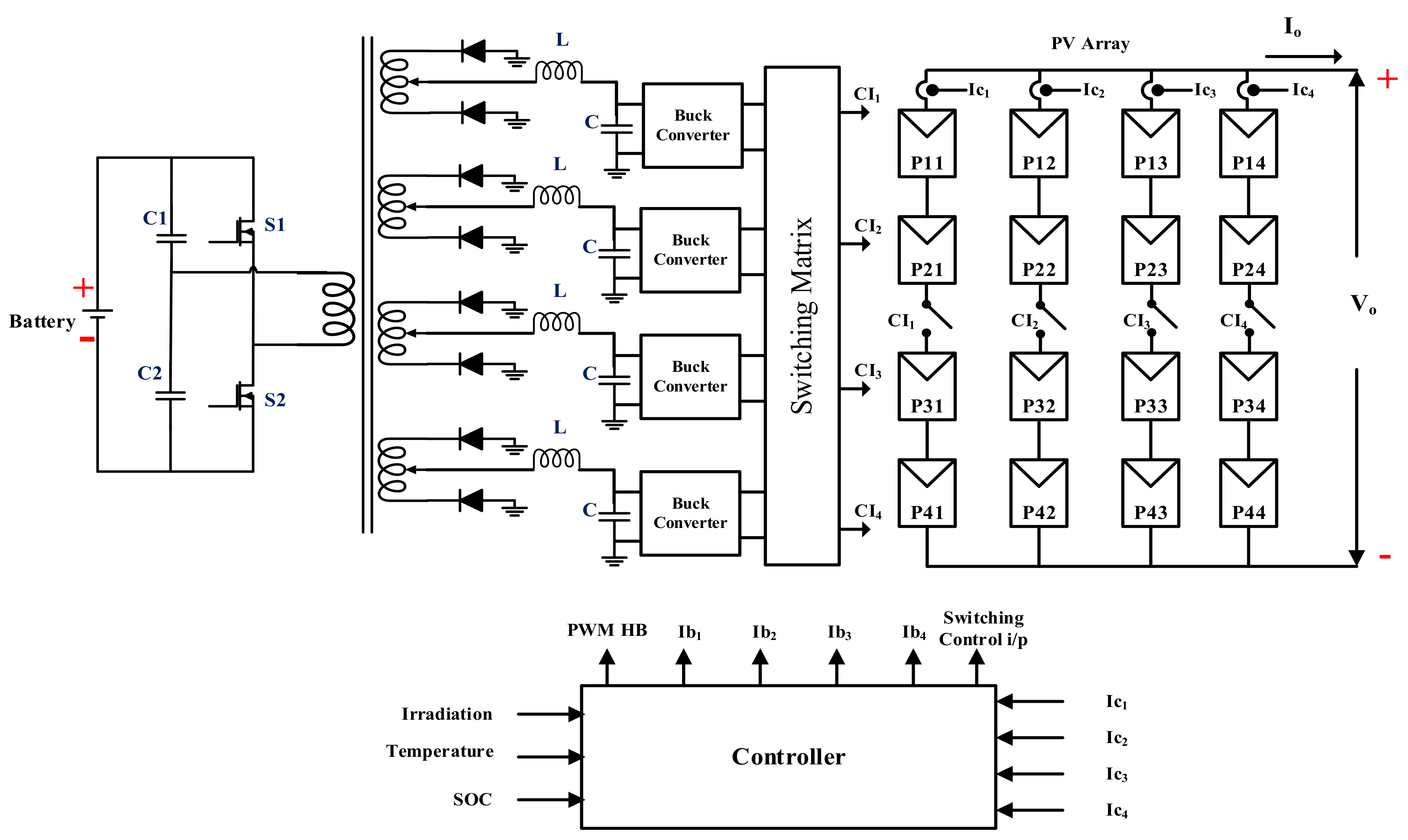
3.2. Implementation of the HBCI Scheme

A simplified switching matrix for a 4 × 4 SP PV array with voltage and current sensing for each module is shown in Figure 6. In addition, a half-bridge isolated current coupled to a DC to DC buck converter is presented. The switching matrix control was compiled in the controller and the controller fed necessary control signals to turn on the appropriate switches.

Based on the above-described principle, an algorithm was developed that consists of the following stages for control and compensation.

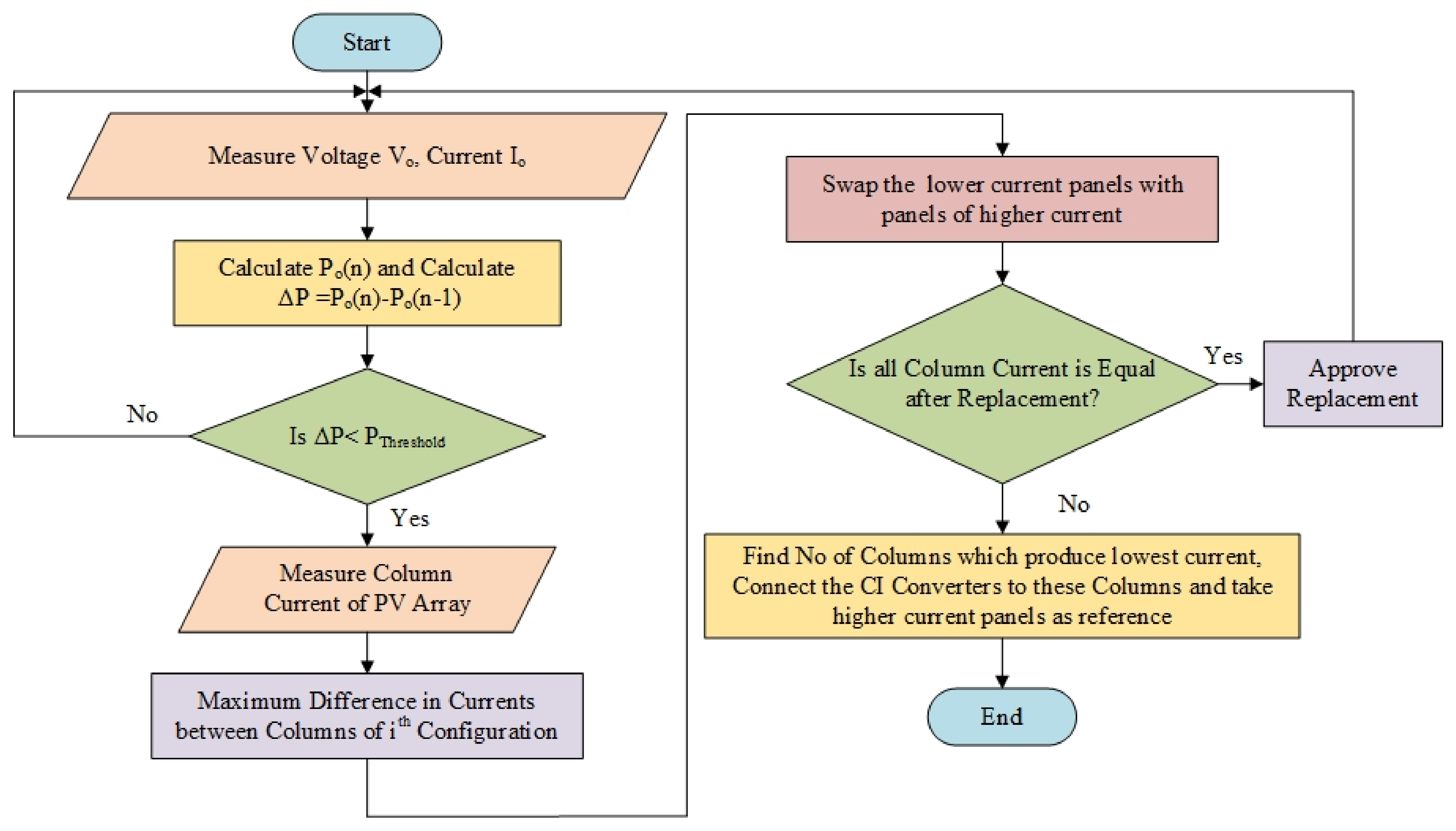
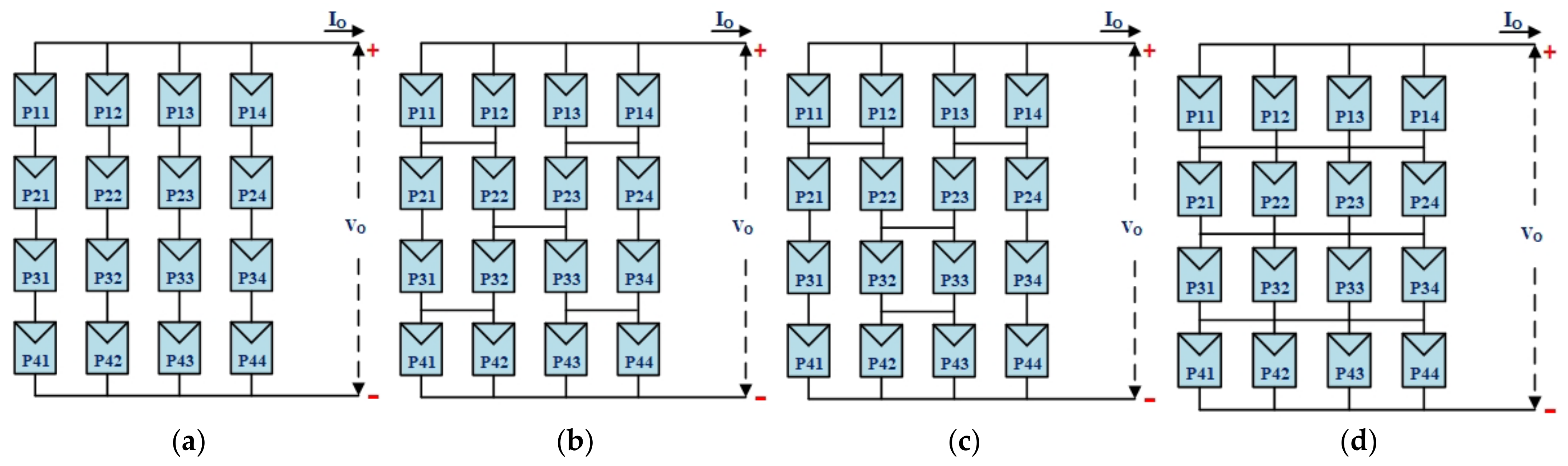
• Step 1: Measure the current and voltage from the 4 × 4 SP array and calculate the power of the PV array as shown in Figure 7a. If power is reduced, then
• Step 2: Calculate the column current of each PV string.
• Step 3: Identify the columns that have the highest and lowest currents.
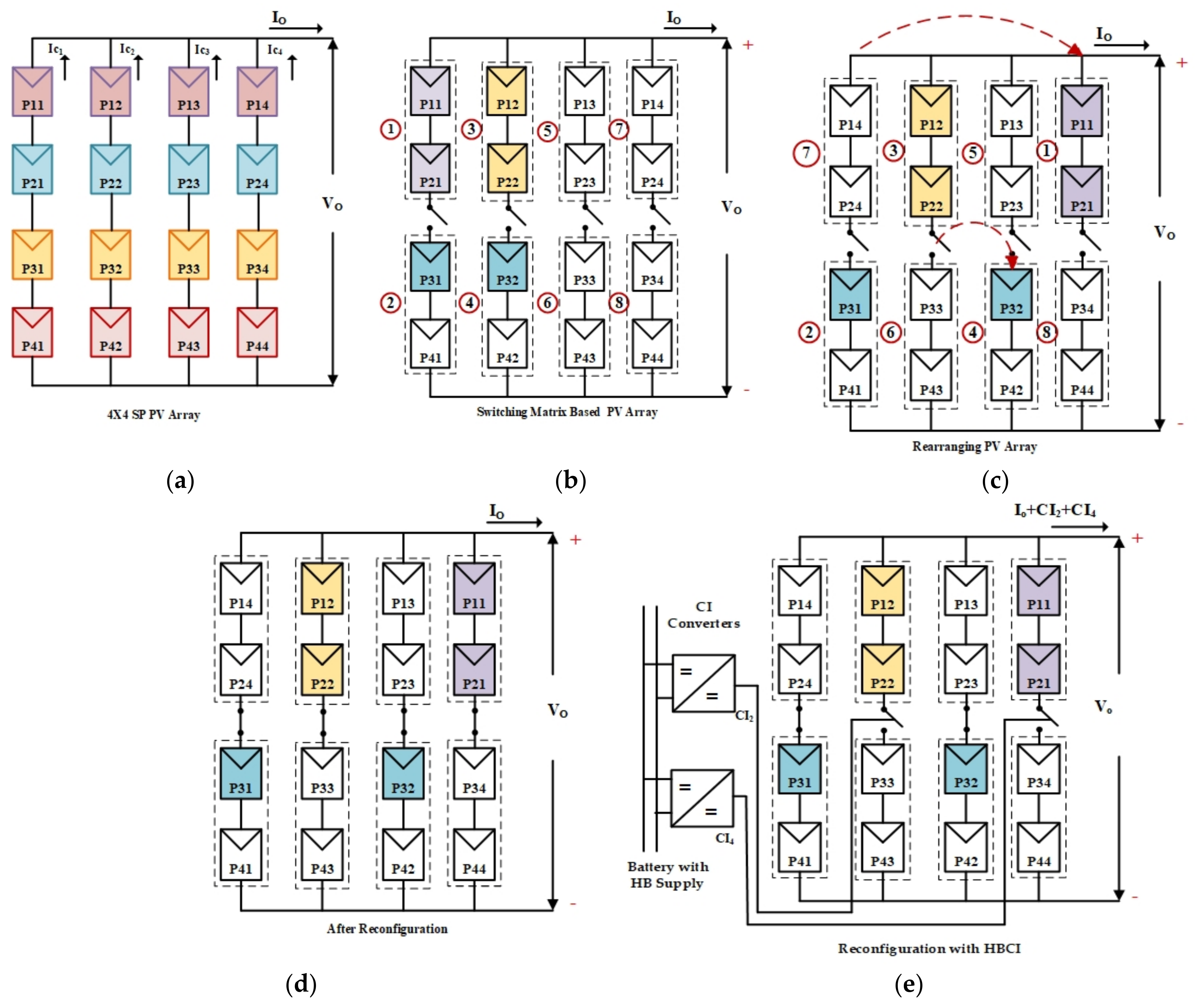
• Step 4: Each of the strings is subdivided into two parts and the whole array is divided into eight parts as shown in Figure 7b.
• Step 5: Swap the panels with lower current with the panels with higher current in any of the columns shown in Figure 7c. Repeat the second and third steps.
• Step 6: If a mismatch still persists between the columns shown in Figure 7d, take the higher current as the reference and apply the current injection method as shown in Figure 7e.

Suppose that, in a PV string, only one panel is shaded. The reconfiguration of the panel is not required; instead, the amount of current that needs to be injected for the shaded panel is squeezed in the column through the power electronic circuit. In the case where more than one panel is shaded, the optimal reconfiguration method is adopted prior to the current injection by the half-bridge current injection setup. The intelligent controller decides the execution of these schemes depending upon the magnitude of the current from the respective string; in fact, the current magnitude is the direct reflection of the quantum of shading.

The number of converter segments needed to inject current into the PV array depends on the string of the PV array. The generic equation describing the required number of converter segments with respect to the array size is given by Equation (4)

$$\mathrm{h}<\left(\mathrm{p} \times \mathrm{q}\right),{ \mathrm{N}}_{\mathrm{k}}=\left(\frac{\mathrm{mod} \left(\frac{\mathrm{h}}{\mathrm{q}}\right)}{\mathrm{p}-\left(\frac{\mathrm{h}}{\mathrm{q}}\right)}\right)$$

(4)

where h refers to the no of shaded modules, p refers to the no of columns, q refers to the no of rows, and N_k refers to the no of converters.

The flow diagram for the HBCI scheme is presented in Figure 8.

3.3. Performance Evaluation Parameters

3.3.1. Mismatching Power Loss (ΔP_L)

The difference between the peak power extracted during homogenous irradiation and the actual power extracted during inhomogeneous irradiation gives the power loss expressed as a percentage [27]. The mismatching power loss is presented in Equation (5)

$$\mathrm{Power} \mathrm{loss}, \Delta {\mathrm{P}}_{\mathrm{L}}\left(\%\right)=\frac{{\mathrm{P}}_{\mathrm{mp}}-{\mathrm{P}}_{\mathrm{sc}}}{{\mathrm{P}}_{\mathrm{mp}}}\times 100$$

(5)

where P_mp denotes the maximum power under homogeneous irradiation conditions and P_sc denotes the maximum power under partial shading conditions.

3.3.2. Fill Factor (FF)

The ratio between the product of the voltage and the current under standard test conditions and the product of the open circuit voltage and the short circuit current gives the fill factor, which is given as an expression in Equation (6)

$$\mathrm{Fill} \mathrm{factor}, \mathrm{FF}=\frac{{\mathrm{V}}_{\mathrm{mp}}{\ast \mathrm{I}}_{\mathrm{mp}}}{{\mathrm{V}}_{\mathrm{oc}}{\ast \mathrm{I}}_{\mathrm{SC}}}\times 100$$

(6)

where V_oc is the open circuit voltage, I_sc is the short circuit current, V_mp is the voltage during the peak output power, and I_mp is the current during the peak output power.

3.3.3. Efficiency (η)

The efficiency is the ratio of the global peak output power to the input solar power and is computed by Equation (7)

$$\mathrm{Efficiency}, \mathsf{\eta }=\frac{{\mathrm{V}}_{\mathrm{mp}}\times {\mathrm{I}}_{\mathrm{mp}}}{I_{si}\times A_{pv}}\times 100$$

(7)

where I_si is the solar intensity per square meter (watt/m²) and A_pv is the area of the PV system (m²).

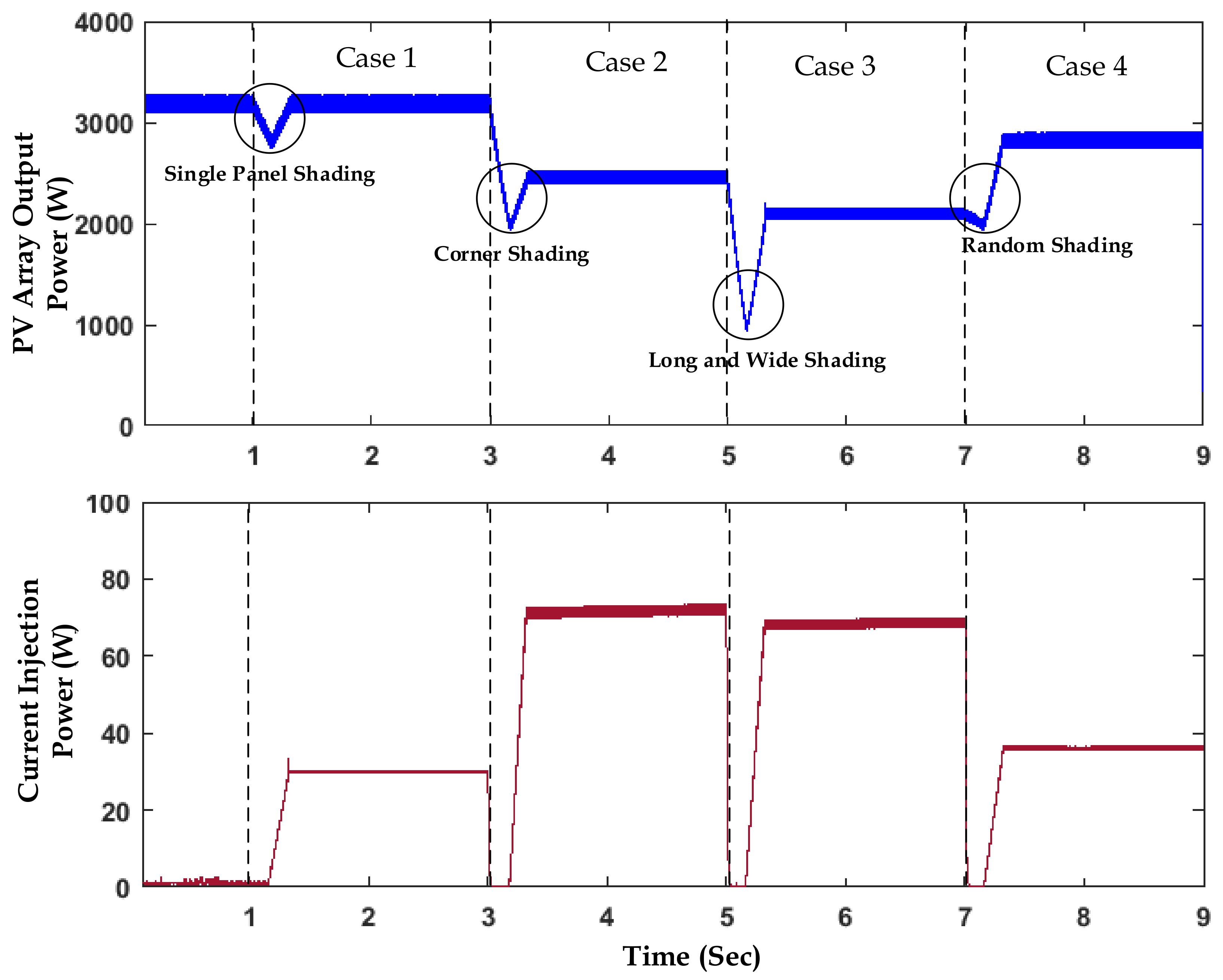
4. Results and Discussions

The schemes proposed in this research work were duly simulated in the Matlab/Simulink environment. The optimal reconfiguration and HBCI schemes were tested in a 4 × 4 SP array subject to shading. The efficacy of the proposed schemes was investigated under various shading conditions, including single-panel shading, corner shading, long and wide shading, and random shading. The proposed HBCI scheme was compared with existing array configurations, including SP, TCT, BL, and HC, and the effectiveness of HBCI was proved. The main attributes, such as the global power peak, power losses, fill factor, and efficiency, were compared.

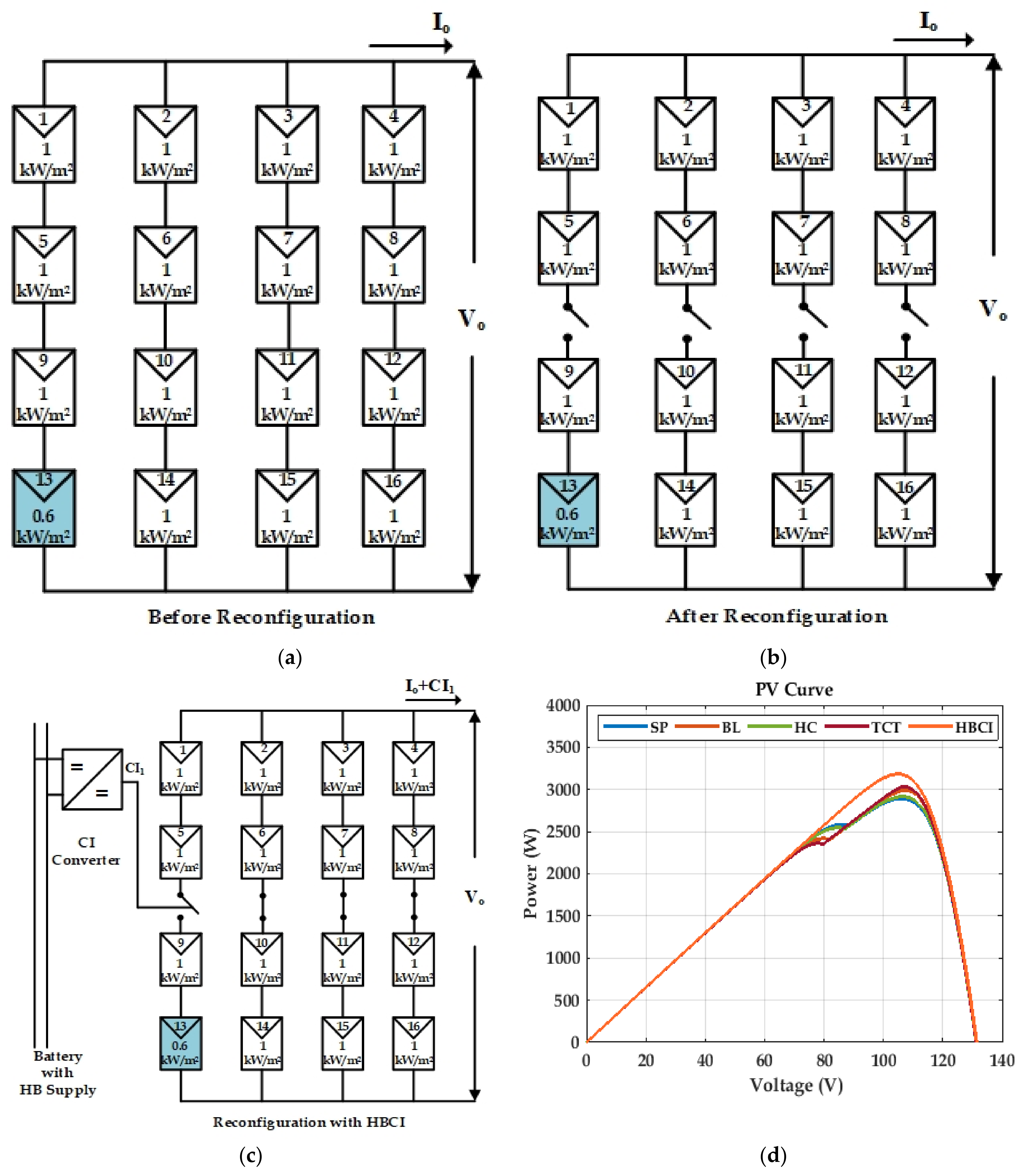
4.1. Case 1: Single-Panel Shading

Consider the case where only one panel is shaded, it receives only 0.6 kW/m², and the remaining 0.4 kW/m² is lost due to shading. This case is clearly presented in Figure 9a. Here, the optimal reconfiguration scheme would not hold, so a current injection through the HBCI technique was performed as shown in Figure 9c. It is worth noting that, due to the single-panel shading, the PV array was able to feed only 2807 W and, after the current injection, the power output increased to 3199 W. Therefore, nearly 392 W of power had been yielded at the cost of injecting 28 W of power from the half-bridge circuit. Figure 9d shows that the HBCI technique has a clear edge over all other techniques by presenting a P-V curve with more power and, more importantly, a single power peak. Under similar shading conditions, the other array configurations (SP, BL, HC, and TCT) possess more bumps in the power curve with a lower global power peak. Furthermore, a detailed analysis of the parameters of the PV array was performed and is presented in

Table 2. Case 1: single-panel shading.

Configuration	Voc (V)	Isc (A)	Vmp (V)	Imp (A)	Pmp (W)	∆PL (%)	FF (%)	η (%)
Series Parallel (SP)	131.3	32.8	98.49	28.51	2807.95	12.25	65.20	12.45
Bridge link (BL)	131.3	32.8	99.57	28.82	2869.607	10.32	66.63	12.72
Honeycomb (HC)	131.3	32.8	98.69	28.57	2819.573	11.89	65.47	12.50
Total Cross Tied (TCT)	131.3	32.8	100.1	28.98	2900.898	9.35	67.36	12.86
HBCI	131.4	32.8	105.2	30.41	3199.132	0.03	74.23	14.18

. The inference from the table is that the proposed scheme outperforms all its counterparts by having less power loss, higher efficiency, and a higher fill factor. It is evident that the HBCI reconfiguration scheme improves the power output and reduces the power losses by 12.22%, 10.30%, 11.86%, and 9.32% with respect to the four conventional configurations SP, BL, HC, and TCT, respectively. Similarly, the fill factor was improved by 9.03%, 7.60%, 8.76%, and 6.87%, respectively, compared with the conventional configurations. Again, the efficiency of the proposed scheme is higher than that of the four configurations by 1.73%, 1.46%, 1.68%, and 1.32%, respectively.

4.2. Case 2: Corner Shading

In this case, a scenario was considered in which six modules are shaded. PV1 and PV2 receive 0.6 kW/m², PV5 and PV6 receive 0.5 kW/m², and PV9 and PV10 receive only 0.3 kW/m². All the other panels receive uniform irradiation of 1kW/m² as illustrated in Figure 10a. Since the panels in an array receive different irradiation levels, the existence of multiple peaks on the P-V output curves is unavoidable. In addition, the power at the output reduces substantially due to shading; suppose that column 1 and column 2 exert the lowest current of 4.088 amps and column 3 and column 4 receive 7.61 amps of current. Therefore, optimal reconfiguration was performed by bifurcating the columns and swapping the panels between the fourth column and the first column. Additionally, the panels in the second and third strings are exchanged as shown in Figure 10b. At the end of this swapping procedure, it was observed that two columns (columns 1 and 3) had the highest current value (6.138 amps) and the other two columns (columns 2 and 4) had the lowest current value (4.857 amps). There exists a current difference even after reconfiguration was completed. Therefore, the intervention of HBCI was required and a deficit current of 2.562 A was injected into column 2 and column 4 as shown in Figure 10c. As a result, the power output was increased from 1970 W to 2536 W. The estimated global maximum power point was also validated by plotting the simulated PV characteristics and is shown in Figure 10d. Under similar shading conditions, the other array configurations (SP, BL, HC, and TCT) are also plotted. Furthermore, the parameters V_oc, V_mp, I_sc, I_mp, and P_mp were analyzed and are presented in

Table 3. Case 2: corner shading.

Configuration	Voc (V)	Isc (A)	Vmp (V)	Imp (A)	Pmp (W)	∆PL (%)	FF (%)	η (%)
Series parallel (SP)	129.9	32.7	82.5	23.88	1970.1	38.43	46.38	8.73
Bridge link (BL)	129.9	32.7	81.36	23.55	1916.028	40.12	45.11	8.49
Honeycomb (HC)	129.9	32.7	81.96	23.72	1944.091	39.25	45.77	8.62
Total cross tied (TCT)	130	32.7	80.53	23.31	1877.154	41.34	44.16	8.32
HBCI	130.2	27	99.86	25.4	2536.444	20.74	72.15	11.24

. It is understood that the HBCI reconfiguration scheme improves the power output by 22.3%, 24.4%, 23.3%, and 25.9% over the conventional schemes, respectively. The power losses by SP, BL, HC, and TCT account for nearly 17.69%, 19.38%, 18.51%, and 20.60% more than that by HBCI. Again, the HBCI scheme improves the fill factor by 25.77%, 27.04%, 26.38%, and 27.99% and improves the efficiency by 2.51%, 2.75%, 2.62%, and 2.92% compared with the SP, BL, HC, and TCT array configurations, respectively. The table also reveals the edge that HBCI has compared with other reconfiguration schemes in terms of fill factor and efficiency.

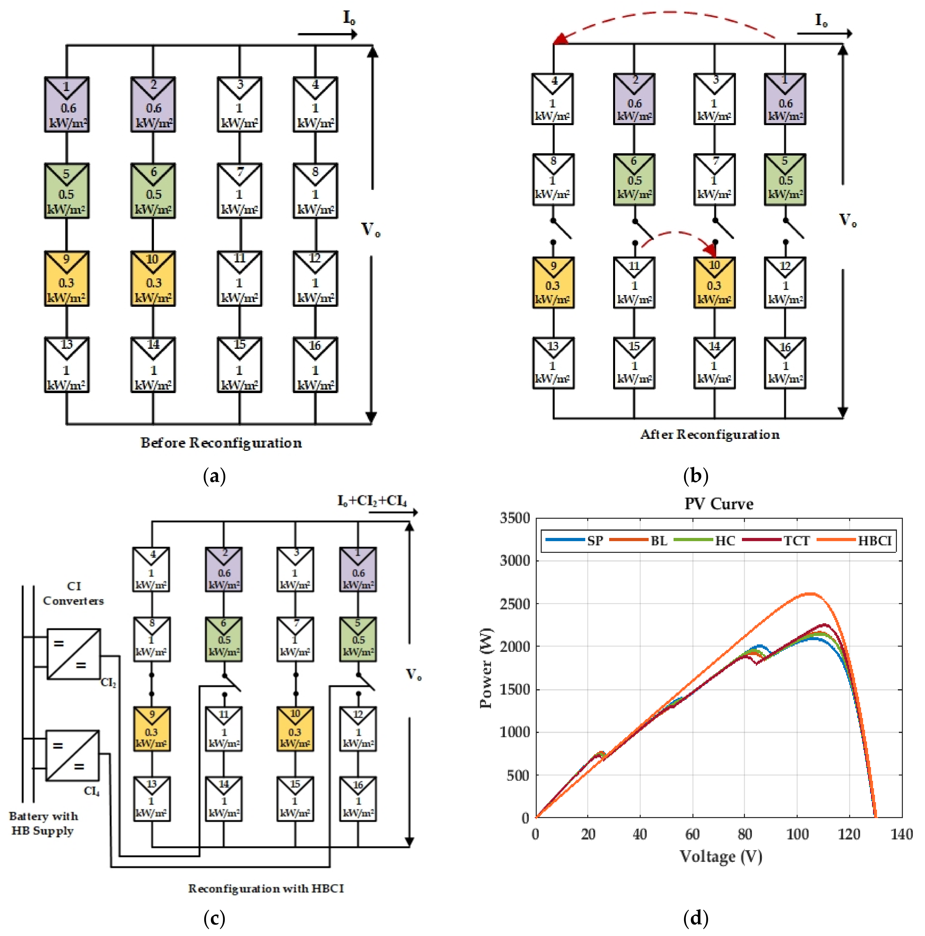
4.3. Case 3: Long and Wide Shading

As illustrated in Figure 11a, almost 12 modules were shaded, where PV1, PV2, PV5, and PV6 received 0.3 kW/m², PV3 and PV7 received 0.4 kW/m², PV9 and PV10 received 0.5 kW/m², PV13 and PV14 received 0.6 kW/m², and PV11 and PV15 received 0.7 kW/m². All the other panels received 1000 W/m². Due to the various levels of insolation, multiple peaks occurred in the PV curve and the power output was reduced. Column 1 and column 2 received the lowest current value (3.788 amps), column 3 received 4.055 amps, and column 4 received 7.61 amps. Therefore, the optimal reconfiguration procedure was adopted by bifurcation of the columns and some of the panels were swapped between column 2 and column 4. The second column had a higher current (4.857 amps) and the other three columns had lower currents (3.788 amps, 4.055 amps, and 4.139 amps) as shown in Figure 11b. The affected columns were injected with current by using the HBCI converters to inject a sufficient amount of current (2.539 amps) as shown in Figure 11c. This helped to achieve the maximum output power in the array from 973 W to 2282 W as shown in Figure 11d. It is evident that the HBCI reconfiguration scheme improves the power output by 57.3%, 57.9%, 57.3%, and 59.2%, reduces the power losses by 40.93%, 41.37%, 40.94%, and 42.30%, improves the fill factor by 37.16%, 37.63%, 37.17%, and 38.61%, and improves the efficiency by 5.81%, 5.87%, 5.81%, and 6.00% compared with the SP, BL, HC, and TCT array configurations, respectively. Again, a comparative analysis shows that HBCI performs better than the other conventional reconfiguration schemes (

Table 4. Case 3: long and wide shading.

Configuration	Voc (V)	Isc (A)	Vmp (V)	Imp (A)	Pmp (W)	∆PL (%)	FF (%)	η (%)
Series parallel (SP)	128.2	23.7	57.99	16.78	973.0722	69.59	32.03	4.31
Bridge link (BL)	128.2	23.7	57.56	16.66	958.9496	70.03	31.56	4.25
Honeycomb (HC)	128.2	23.7	57.98	16.78	972.9044	69.60	32.02	4.31
Total cross tied (TCT)	128.2	23.7	56.66	16.4	929.224	70.96	30.58	4.12
HBCI	129.9	25.4	92.12	24.78	2282.734	28.66	69.19	10.12

).

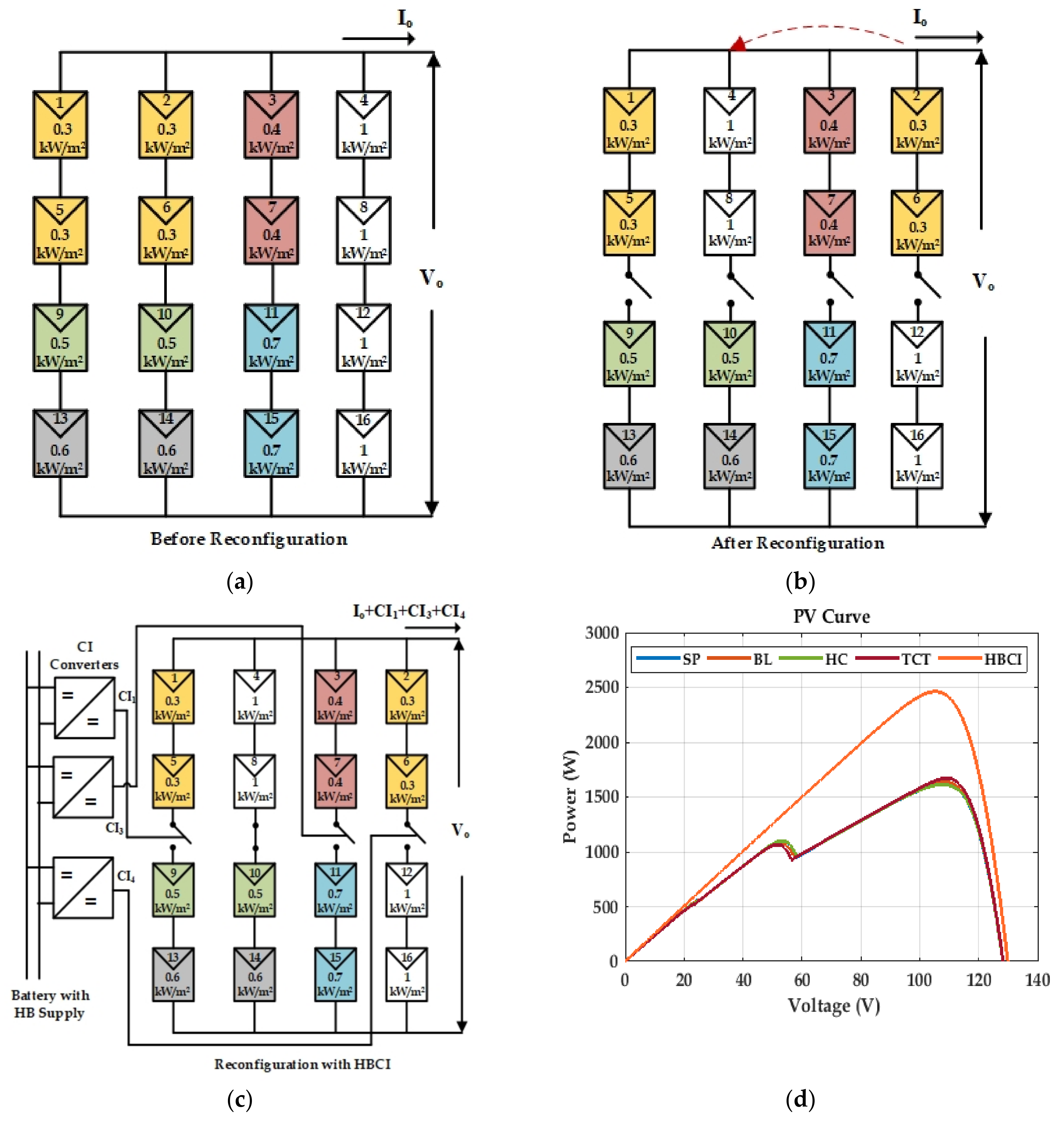
4.4. Case 4: Random Shading

In this case, random shading was considered where nine modules are randomly shaded. PV2, PV15, and PV16 received 0.9 kW/m², PV9 and PV10 received 0.8 kW/m², PV5, PV11, and PV12 received 0.7 kW/m², PV4 received 0.7 kW/m², and all other panels received 1 kW/m² as shown in Figure 12a. The existence of multiple power peaks and power losses are inevitable. The shading pattern was arranged in such a way that column 2 had the highest current (6.787 amps) and column 1, column 3, and column 4 had low current values (5.832 amps, 6.044 amps, and 5.102 amps, respectively). The reconfiguration and current injection schemes were systematically applied and the results are duly presented in Figure 12b,c. With the help of the half-bridge-driven buck converter circuit, the required amount of current (1.761 amps) was injected and the output power after the injection of current increased from 2028 W to 2810 W. Excluding the converter losses of 36 W, the net array output power amounts to 2774 W. The estimated global maximum power point was validated by plotting the simulated PV characteristics and is shown in Figure 12d. Under similar shading conditions, the other array configurations (SP, BL, HC, and TCT) are also plotted. Furthermore, the parameters V_oc, V_mp, I_sc, I_mp, and P_mp were calculated and are displayed in

Table 5. Case 4: random shading.

Configuration	Voc (V)	Isc (A)	Vmp (V)	Imp (A)	Pmp (W)	∆PL (%)	FF (%)	η (%)
Series parallel (SP)	130.6	32.7	83.72	24.23	2028.536	36.61	47.50	9.00
Bridge link (BL)	130.6	31.9	82.34	24.2	1992.628	37.73	47.83	8.83
Honeycomb (HC)	130.6	32.7	83.64	24.21	2024.924	36.72	47.42	8.98
Total cross tied (TCT)	130.6	31	84.84	24.56	2083.67	34.89	51.47	9.24
HBCI	130.8	29.5	99.04	28.38	2810.755	12.16	72.84	12.46

. It is evident that the HBCI reconfiguration scheme improves the power output by 27.8%, 29.1%, 27.9%, and 25.8%, reduces the power losses by 24.45%, 25.57%, 24.56%, and 22.73%, improves the fill factor by 25.34%, 25.01%, 25.42%, and 21.37%, and improves the efficiency by 3.46%, 3.63%, 3.48%, and 3.22% compared with the SP, BL, HC, and TCT array configurations, respectively.

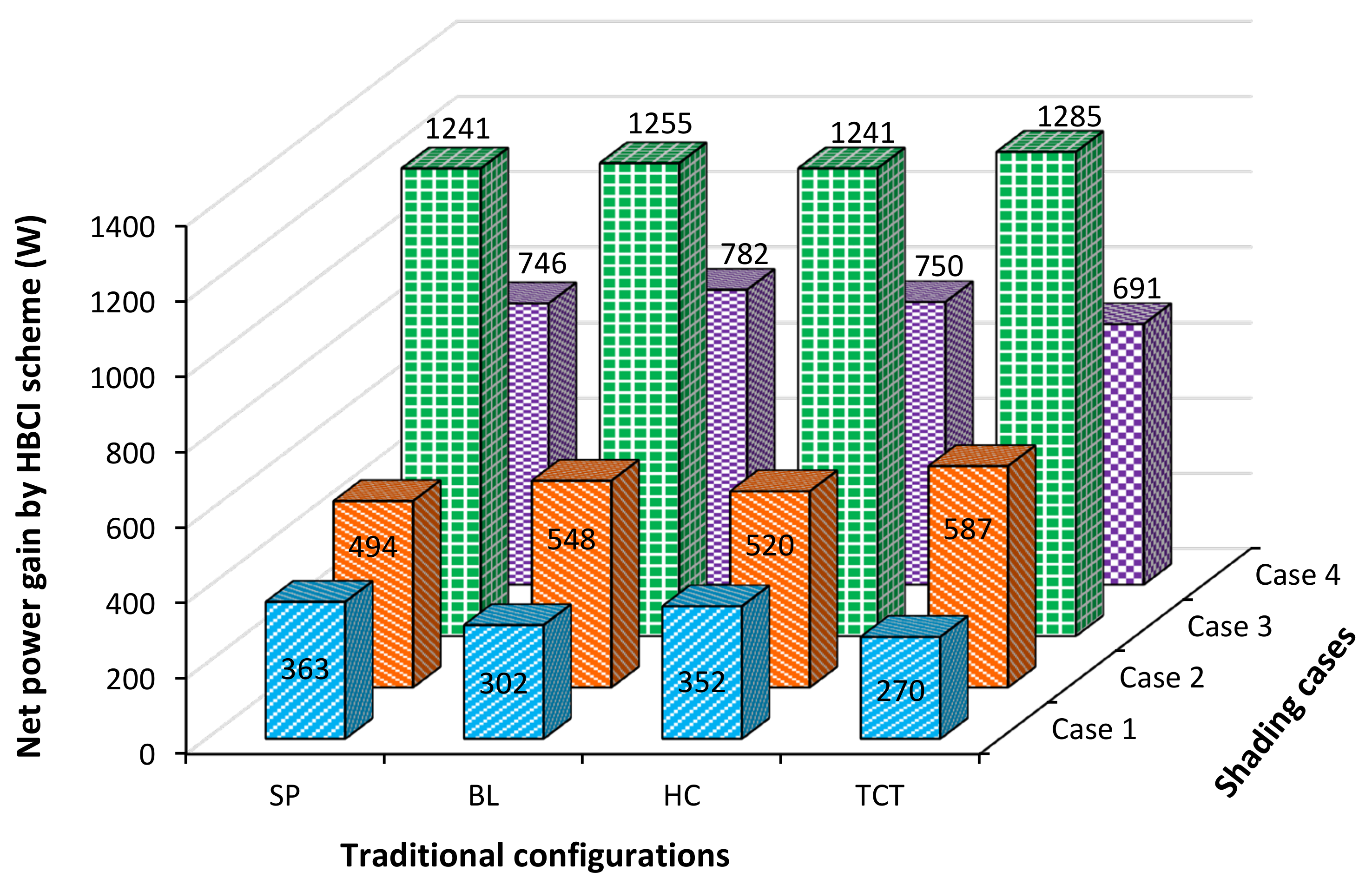
4.5. Comparison of the Cases

The versatility and the reliability of the proposed scheme are evident from Figure 13, where the shading cases and the response of the converter with the current injection are duly presented. In Case 1, where a single panel is shaded, the output power was reduced to 2807 W and the controller responded immediately by feeding a control signal to the half-bridge converter, which enabled the current injection. The HBCI converter started to inject the remaining current into the affected columns. The output power was increased to 3199 W and, under this condition, the HBCI converter’s power consumption was only 28 W. In the second case, in which the shading happened in the corner area, the output power fell to 1970 W. Under this condition, the controller measured the column current and the mismatch in available current between the columns; then, the optimal reconfiguration was adopted and the remaining current was injected through the HBCI converters. The output power increased to 2536 W. Likewise, under long and wide shading conditions, the HBCI converter injected 69 W to improve the output power to 2282 W. Similarly, in the fourth case, in which random shading occurred, the power dropped to 2028 W and, due to the HBCI, the power then increased to 2810 W. All the probable conditions were tested, and it is evident that the output power from the PV array increased and the performance of the whole system improved.

Compensation was effectively provided for by the HBCI and a higher power yield was acquired for all the shading cases. On the other hand, the HBCI consumed only a small amount of power to generate a good power yield. For example, in Case 1 with the SP configuration, during shading the power loss was nearly 392 W. The HBCI consumed 28 W in the process of compensating for 392 W and a net power gain of 364 W was yielded. Figure 14 presents the net power gain of the shaded PV array for different cases compared to different traditional configurations. This net power gain was calculated by subtracting the power outputs of all four configurations during shading and the HBCI power consumptions for compensating for the HBCI output power. The quantification on the positive net power gain clearly shows that HBCI was superior to all its counterparts.

The system does not suffer from the limitation with respect to the control approach with different PV tracking options when the PV system is connected to the grid. The PV maximum power tracking options need not be different; the conventional power tracking schemes, such as perturb and observe (P&O) and incremental conductance (INC), are sufficient as the compensation proposed here will provide uniform P-V and I-V curves.

In this work, the single-diode PV model was used to implement the proposed current injection scheme. However, double-diode model (DDM) and triple-diode model (TDM) equivalent circuits can also be found in the literature, and they involve more parameters, which would improve the modeling accuracy [28,29]. In the future, the DDM or the TDM could be considered to further validate the system’s applicability.

4.6. Cost–Benefit Analysis

The investment in the HBCI unit will cost around $50 for a 3.5 KW PV system. Due to the shading, the power–voltage (P-V) curves will have multiple power peaks, the MPPT employed may only track the local power peak, and the remaining power may be lost. In this work, four cases of differential shading were tested on a PV array and losses with and without the proposed scheme were analyzed. The results are duly tabulated in

Table 6. Power comparison with and without HBCI.

Cases	MPPT without HBCI	MPPT with HBCI
Case 1	2807.95 W	3199.13 W
Case 2	1877.15 W	2536.44 W
Case 3	929.22 W	2282.73 W
Case 4	1992.62 W	2810.75 W
Total	7606.94	10,829.05

.

The inference from the cost–benefit analysis is that, on average, 3.2 units of energy are lost per day, which accounts for a monetary loss of nearly $0.5 a day. Over a period of 5 years, nearly $912 can be saved by the proposed HBCI. In addition, the PV panels will succumb to continuous shading, and the competence of the MPPT controller will surely be affected over this time period.

The additional expected cost for the half-bridge converter, the buck converter, the battery, and the controller would be approximately $150 for implementing the system, but the investment is worth making as it reduces the power losses by 42.30% in the worst-case shading scenario. More importantly, only by the current injection scheme proposed here do the P-V curves have a single peak, which can be managed by the existing MPPT schemes. However, without the proposed current injection scheme, the P-V curves would have multiple power peaks, which require further investment in complex global tracking control schemes.

5. Conclusions

In this work, an energy-storage-embedded half-bridge–buck-converter-aided current injection scheme with an intelligent optimal reconfiguration scheme was proposed for a shaded PV array. The topology of the half bridge is the best fit here since it has multiple power outputs and buck converters are highly compatible with it. To reduce the burden on the current injection circuit when the magnitude of the shading is large, an optimal reconfiguration scheme is adopted wherein the amount of current injection is reduced. The reconfiguration results in the dispersion of the shading over the whole PV array and lessens the required amount of current for compensation. The effectiveness of the proposed scheme under different shading conditions was verified in four cases: single-panel shading, corner shading, long and wide shading, and random shading. The HBCI proved its efficacy by mitigating the average power loss by 9.32% to 42.30%. The average fill factor and the average efficiency of the PV array were improved by 6.87% to 38.61% and 1.32% to 6.00%, respectively. In the future, the proposed scheme can be further enhanced for a PV system with a higher power rating and an appropriate converter topology design.

References

1. Bastidas-Rodriguez, J.D.; Cruz-Duarte, J.M.; Correa, R. Mismatched Series–Parallel Photovoltaic Generator Modeling: An Implicit Current–Voltage Approach. IEEE J. Photovolta. 2019, 9, 768–774. [Google Scholar] [CrossRef]
2. Maki, A.; Valkealahti, S. Effect of Photovoltaic Generator Components on the Number of MPPs under Partial Shading Conditions. IEEE Trans. Energy Convers. 2013, 28, 1008–1017. [Google Scholar] [CrossRef]
3. Ali, A.; Almutairi, K.; Padmanaban, S.; Tirth, V.; Algarni, S.; Irshad, K.; Islam, S.; Zahir, M.H.; Shafiullah, M.; Malik, M.Z. Investigation of MPPT Techniques Under Uniform and Non-Uniform Solar Irradiation Condition—A Retrospection. IEEE Acces 2020, 8, 127368–127392. [Google Scholar] [CrossRef]
4. Wang, S.-C.; Pai, H.-Y.; Chen, G.-J.; Liu, Y.-H. A Fast and Efficient Maximum Power Tracking Combining Simplified State Estimation with Adaptive Perturb and Observe. IEEE Access 2020, 8, 155319–155328. [Google Scholar] [CrossRef]
5. Li, S.; Li, F.; Zheng, J.; Chen, W.; Zhang, D. An improved MPPT control strategy based on incremental conductance method. Soft Comput. 2020, 24, 6039–6046. [Google Scholar] [CrossRef]
6. Deshmukh, N.R. Comparision of Perturb and Observer and Incremental Conductance MPPT Based Solar Tracking System. Int. J. Eng. Res. 2015, 4, 222–223. [Google Scholar] [CrossRef]
7. Li, H.; Yang, D.; Su, W.; Lu, J.; Yu, X. An Overall Distribution Particle Swarm Optimization MPPT Algorithm for Photovoltaic System under Partial Shading. IEEE Trans. Ind. Electron. 2019, 66, 265–275. [Google Scholar] [CrossRef]
8. Manickam, C.; Raman, G.; Ganesan, S.I.; Nagamani, C. A Hybrid Algorithm for Tracking of GMPP Based on P&O and PSO with Reduced Power Oscillation in String Inverters. IEEE Trans. Ind. Electron. 2016, 63, 6097–6106. [Google Scholar] [CrossRef]
9. Tey, K.S.; Mekhilef, S.; Seyedmahmoudian, M.; Horan, B.; Oo, A.T.; Stojcevski, A. Improved Differential Evolution-Based MPPT Algorithm Using SEPIC for PV Systems Under Partial Shading Conditions and Load Variation. IEEE Trans. Ind. Inform. 2018, 14, 4322–4333. [Google Scholar] [CrossRef]
10. Ramasamy, S.; Dash, S.S.; Selvan, T. An Intelligent Differential Evolution based Maximum Power Point Tracking (MPPT) Technique for Partially Shaded Photo Voltaic (PV) Array. Int. J. Adv. Soft Comput. Appl. 2014, 6, 1–16. [Google Scholar]
11. Titri, S.; Larbes, C.; Toumi, K.Y.; Benatchba, K. A new MPPT controller based on the Ant colony optimization algorithm for Photovoltaic systems under partial shading conditions. Appl. Soft Comput. 2017, 58, 465–479. [Google Scholar] [CrossRef]
12. Sridhar, R.; Jeevananthan, S.; Dash, S.S.; Vishnuram, P. A new maximum power tracking in PV system during partially shaded conditions based on shuffled frog leap algorithm. J. Exp. Theor. Artif. Intell. 2016, 29, 481–493. [Google Scholar] [CrossRef]
13. Arulmurugan, R. Optimization of Perturb and Observe Based Fuzzy Logic MPPT Controller for Independent PV Solar System. WSEAS Trans. Power Syst. 2020, 19, 159–167. [Google Scholar] [CrossRef]
14. Rahman, M.M.; Islam, M.S. PSO and ANN Based Hybrid MPPT Algorithm for Photovoltaic Array under Partial Shading Condition. Eng. Int. 2020, 8, 9–24. [Google Scholar] [CrossRef]
15. Ulaganathan, M.; Devaraj, D. A novel MPPT controller using Neural Network and Gain-Scheduled PI for Solar PV system under rapidly varying environmental condition. J. Intell. Fuzzy Syst. 2019, 37, 1085–1098. [Google Scholar] [CrossRef]
16. Manjunath Suresh, H.N.; Rajanna, S. Performance Enhancement of Hybrid Interconnected Solar Photovoltaic Array Using Shade Dispersion Magic Square Puzzle Pattern Technique under Partial Shading Conditions. Sol. Energy 2019, 194, 602–617. [Google Scholar] [CrossRef]
17. Deng, S.; Zhang, Z.; Ju, C.; Dong, J.; Xia, Z.; Yan, X.; Xu, T.; Xing, G. Research on hot spot risk for high-efficiency solar module. Energy Procedia 2017, 130, 77–86. [Google Scholar] [CrossRef]
18. Venkateswari, R.; Sreejith, S. Factors influencing the efficiency of photovoltaic system. Renew. Sustain. Energy Rev. 2019, 101, 376–394. [Google Scholar] [CrossRef]
19. Bingöl, O.; Özkaya, B. Analysis and comparison of different PV array configurations under partial shading conditions. Sol. Energy 2018, 160, 336–343. [Google Scholar] [CrossRef]
20. Sai Krishna, G.; Moger, T. Improved SuDoKu Reconfiguration Technique for Total-Cross-Tied PV Array to Enhance Maximum Power Under Partial Shading Conditions. Renew. Sustain. Energy Rev. 2019, 109, 333–348. [Google Scholar] [CrossRef]
21. Bonthagorla, P.K.; Mikkili, S. Performance investigation of hybrid and conventional PV array configurations for grid-connected/standalone PV systems. CSEE J. Power Energy Syst. 2020. [Google Scholar] [CrossRef]
22. Karmakar, B.K.; Karmakar, G. A Current Supported PV Array Reconfiguration Technique to Mitigate Partial Shading. IEEE Trans. Sustain. Energy 2021, 12, 1449–1460. [Google Scholar] [CrossRef]
23. Alkahtani, M.; Wu, Z.; Kuka, C.S.; Alahammad, M.S.; Ni, K. A Novel PV Array Reconfiguration Algorithm Approach to Optimising Power Generation Across Non-Uniformly Aged PV Arrays by Merely Repositioning. Multidiscip. Sci. J. 2020, 3, 5. [Google Scholar] [CrossRef] [Green Version]
24. Bendary, A.; Abdelaziz, A.; Ismail, M.; Mahmoud, K.; Lehtonen, M.; Darwish, M. Proposed ANFIS Based Approach for Fault Tracking, Detection, Clearing and Rearrangement for Photovoltaic System. Sensors 2021, 21, 2269. [Google Scholar] [CrossRef]
25. Prince Winston, D.; Kumaravel, S.; Praveen Kumar, B.; Devakirubakaran, S. Performance Improvement of Solar PV Array Topologies during Various Partial Shading Conditions. Sol. Energy 2020, 196, 228–242. [Google Scholar] [CrossRef]
26. Keerti, Y.; Anuprita, M. Analysis and Modeling of Photo-Voltaic (PV) Cell Power Generation System Using Simulink. Int. J. Recent Trends Eng. Res. 2018, 4, 128–135. [Google Scholar]
27. Sharma, H.; Kumar, P.; Patra, J. Performance Analysis of Different PV Topologies with MPPT. Int. J. Trend Sci. Res. Dev. 2017, 1, 656–664. [Google Scholar] [CrossRef]
28. Said, M.; Shaheen, A.M.; Ginidi, A.R.; Sehiemy, R.A.E.; Mahmoud, K.; Lehtonen, M.; Darwish, M.M.F. Estimating Parameters of Photovoltaic Models Using Accurate Turbulent Flow of Water Optimizer. Processes 2021, 9, 627. [Google Scholar] [CrossRef]
29. Naeijian, M.; Rahimnejad, A.; Ebrahimi, S.M.; Pourmousa, N.; Gadsden, S.A. Parameter estimation of PV solar cells and modules using Whippy Harris Hawks Optimization Algorithm. Energy Rep. 2021, 7, 4047–4063. [Google Scholar] [CrossRef]
Figure 1. Different PV array configurations: (a) series parallel; (b) bridge link; (c) honeycomb; (d) total cross tied.
Energies 14 06332 g001
Figure 2. The single-diode PV model.
Energies 14 06332 g002
Figure 3. Equivalent circuit of a PV array.
Energies 14 06332 g003
Figure 4. (a) Shaded SP PV array; (b) PV curve for uniform irradiation; (c) PV curve for nonuniform irradiation.
Energies 14 06332 g004
Figure 5. (a) Optimal reconfiguration scheme for a shaded PV array; (b) Half-Bridge Current Injection (HBCI) scheme.
Energies 14 06332 g005
Figure 6. Implementation of the HBCI Scheme.
Energies 14 06332 g006
Figure 7. (a) The 4 × 4 SP PV array; (b) the switching matrix-based PV array; (c) rearranging the PV array; (d) after reconfiguration; (e) reconfiguration with Half-Bridge Current Injection (HBCI).
Energies 14 06332 g007
Figure 8. Algorithm for the Half-Bridge Current Injection (HBCI) scheme.
Energies 14 06332 g008
Figure 9. Case 1: single-panel shading: (a) the SP array configuration; (b) after reconfiguration with HBCI; (c) reconfiguration with HBCI; (d) PV characteristics.
Energies 14 06332 g009
Figure 10. Case 2: corner shading: (a) the SP array configuration; (b) after reconfiguration with HBCI; (c) reconfiguration with HBCI; (d) PV characteristics.
Energies 14 06332 g010
Figure 11. Case 3: long and wide shading: (a) the SP array configuration; (b) after reconfiguration with HBCI; (c) reconfiguration with HBCI; (d) PV characteristics.
Energies 14 06332 g011
Figure 12. Case 4: random shading: (a) the SP array configuration; (b) after reconfiguration with HBCI; (c) reconfiguration with HBCI; (d) PV characteristics.
Energies 14 06332 g012
Figure 13. HBCI power output and power consumption during the injection of current for the shading cases (Note: the different schemes have a 2 s gap).
Energies 14 06332 g013
Figure 14. Net power gain by the proposed reconfiguration and the HBCI scheme compared to the traditional schemes (SP, series parallel; BL, bridge link; HC, honeycomb; TCT, total cross tied) for different cases (single panel, corner, long and wide, random) of PV array shading (net power gain = HBCI power output-power output by a traditional scheme-HBCI power consumption).
Energies 14 06332 g014