1. Introduction
Modern seismic processing and interpretation is focused on improving the evaluation of hydrocarbon prospection on the basis of detecting lithology and fluid anomalies. Novel seismic workflows combine AVO analysis and inversion technology, and derive relative elastic property attributes—for example, P- and S-wave impedance and Vp/Vs ratio [
1]. Seismic data after processing and structural interpretation are used in preparing reconstructed models of petroleum systems based on paleogeological cross-sections [
2]. Well logging outcomes, i.e., measured logs and results of the petrophysical interpretation, as well as geochemical information are also useful and included in the models. Continuous cooperation between seismic and well logging teams is always related to including new concepts in velocity model building, novelties in acoustic borehole measurements—modern, sophisticated devices—and professional—commercial and specialized domestic—software. Chiu and Stewart [
3] developed a tomographic technique, i.e., travel time inversion, to determine the 2D or 3D velocity structure of rock formation, combining well logs, vertical seismic profiles, and surface seismic measurements. Silva and Stovas [
4] used high-frequency sonic log data to compare velocity estimation from methods using linear or quadratic models from Taylor series to estimate velocity as a function of depth. The analysis showed that the velocity models preserving the travel time parameters were better as regards accuracy than others. Jarzyna et al. [
5,
6] proved that using novel acoustic devices for borehole measurement and applying software dedicated to specialized processing provided more precise velocity information for seismic processing and interpretation. Huang and Zhang [
7] efficiently used statistical methods to automatically build an initial velocity model and optimized the final result with quantified uncertainty.
Expectations for well logging in the face of modern seismic procedures are increasing. Standard sonic and density or litho-density logs do not provide enough exact data for requested velocity models, especially in poor borehole conditions, where great increases in borehole diameter—caves or washouts—are observed.
In the deep D-1 borehole, located in the central part of the Polish Outer Carpathians area of complex geological structure, a few sonic logs were available. They were as follows: raw and corrected P-wave slowness from standard sonic logging—DT and DTc, respectively; synthetic P-wave slowness based on the litho-porosity–saturation petrophysical interpretation—sDT; P- and S-wave slowness from the full waveform sonic logging—DTP and DTS, respectively. None of the available acoustic logs in the borehole fitted a regional velocity model that had been constructed for the prospective area. The main problem reported by the seismic group, who cooperate in the investigated area, was the quality of the available acoustic logs in the D-1 borehole:
The velocity obtained from DTc and sDT curves in many depth intervals did not fit the interval velocity from the Check Shot (CS) measurement.
In the shallow part of the D-1 borehole, the DTc log presented an overly low P-wave velocity and also overly high contrasts at the boundaries between the reservoir sandstones horizons and interbedded shales. These sections correlated with significant caliper enlargements, so the problem with the DTc curve was related to the poor borehole conditions and thus poor quality of sonic logging.
On the contrary, sDT log presented overly high P-wave velocity in comparison to the interval velocity from the CS. This log was also very smoothed and gave overly low contrasts of velocity between the sandstones and shales. As a result, the amplitudes on the synthetic seismograms were either too high for DTc or too small for sDT, and did not agree with the real seismic trace derived from the borehole location.
DTP and DTS, although of very good quality, were performed only in the deeper sections of the D-1 borehole.
The paper presents two methods, multiple regression (MR) and a modified Faust equation, used for modeling a velocity log on the basis of available well logging data in the D-1 borehole. Several approaches are described where well logging solutions are set together with the geological information on lithology, stratigraphy, and tectonics. Velocity determined from CS surveys, as well as synthetic seismograms computed from the velocity models based on well logging data compared with the real seismic recordings, are also included. The presented case study shows the importance of effective cooperation between interpreters of seismic and well logging data. It also reveals that the proven statistical techniques made the archival data still useful.
2. Geological Settings
Presented solutions were obtained in the D-1 borehole located in the central part of the Silesian Unit, one of the main structural units of the Polish Outer Carpathians (
Figure 1). The Silesian Unit is composed of a sedimentary succession that is over 4000 m thick, encompassing the Lower Cretaceous to Miocene deposits. The sedimentary succession includes mainly flysch formation—sandstones and shales. In
Figure 1, attention is focused on the tectonic units, assuming that the lithology is similar.
Figure 2 presents a regional seismic section along the T-2 profile. The D-1 borehole drilled two thrust-folds of the Silesian Unit: the structurally upper Iwonicz Zdrój (IZ) Fold and structurally lower Osobnica–Bóbrka–Rogi (OBR) Fold. The lithostratigraphic profile of the borehole is presented in
Table 1.
The IZ Fold is the southernmost structural element of the Silesian Unit. The fold was generated as a result of internal detachment in the middle part of the Silesian stratigraphic sequence, encompassing the Istebna Beds and Eocene sediments, and this part of the sequence is situated toward NE on the southern limb of the next thrust-fold, i.e., the OBR Fold. The youngest, syn-orogenic deposits of the Silesian sequence, i.e., the Krosno Beds, adapted to the growing folds and were deformed in a passive roof duplex [
9,
10,
11]. The IZ and OBR Folds have a NW–SE strike and are divided into several blocks by transverse faults more or less perpendicular to the strike direction [
12]. The folds have a well-developed frontal anticline and southern limb displaying a homoclinal sequence of layers with only a few internal deformations.
Both folds are composed of a similar sequence of sedimentary formations (
Table 1). A continuous sequence of their limbs is built of the Upper Cretaceous/Paleocene Istebna Beds and the Paleocene–Eocene Ciężkowice Sandstones interbedded with the Variegated Shales, which are followed by the Oligocene Menilite and the Transitional Beds (
Table 1). The thickness of the Variegated Shales intervals in the upper and lower folds is comparable, and the same applies to the Ciężkowice Sandstones intervals.
Several hydrocarbon horizons occur in the sandstone complexes of the Ciężkowice Sandstones and the Istebna Beds, and both lithostratigraphic units are regarded as the best reservoir formations of the Carpathians. Sealing is provided by the Variegated Shales, which are mostly composed of clay shales, rarely intercalated by sandstones. The hydrocarbon reservoirs are also partly tectonically sealed by faults and overthrusts [
13].
The macroscopic description of cores [
8] and mineral components from the petrophysical interpretation of well logs revealed four main lithological types of the investigated rocks, i.e., shales, sandstones, mudstones, and marls. The considered rocks represent typical flysch sediments observed in the Carpathians, accumulated in the different parts of the Silesian sedimentary basin and subjected to tectonic activity that resulted in different petrophysical properties.
Various statistical analyses preceding these studies were performed in all lithostratigraphic units and predicted quantities were determined in the full geological profile of the D-1 borehole to enhance the petrophysical recognition of the rocks. More detailed information is presented in the paper for the Variegated Shales and the Ciężkowice Sandstones, both consisting of four interlayered intervals. The precise analyses of these formations are included in the following sections, because the depositional age, position, and facies type influenced their petrophysical properties [
14,
15].
3. Data in the Study
Several groups of data were analyzed in this study. For this research, we selected the logs described in
Table 2. Our selection criteria were: good quality of the measurements, availability in the full depth interval, and logs that had a mutual relationship with the velocity logs (i.e., the most informative in the problem of velocity). Moreover, in the analyses, we included the macroscopic description of cores retrieved from the borehole in the drilling process, and results of laboratory measurements on plugs [
8]. Check Shot data were also analyzed, providing the independent seismic velocity model.
3.1. Well Logging Data
Well logging data were acquired in depth intervals according to the drilling operation in the borehole, with various bit sizes in each section. Information on selected well logs measured in the D-1 borehole is presented in
Table 2. All well logs were gathered with a 0.1 m sampling rate.
Well logging results are ideal for statistical analyses because of the large amount of data. Raw log data were preprocessed to remove environmental influences such that they only reflected petrophysical properties. For instance, gamma ray and spectral gamma ray, neutron, and density logs were corrected for borehole conditions, and the transit interval time from the sonic log was corrected for cycle skipping. The c letter added to the standard mnemonics, e.g., GRc, indicates corrected values.
All logs were used in the full petrophysical interpretation to solve for mineral composition, porosity, and water/hydrocarbon saturation. Litho-porosity–saturation solution was obtained on the basis of the mixed lithological components. The solution reflects the difficulties in adopting an appropriate lithology in the geological profile of flysch sediments and differentiating between shales, sandstones, mudstones, and marls. Qz, Ca, and Do mean the presence of quartz as the main mineral of the framework component, calcite and dolomite as important components of cement in sandstones and mudstones, and as the main minerals in marls. Selection of correct minerals in the interpretation of well logs allowed the adjustment of proper framework parameters. Next, the rock-frame parameters were applied to the calculation of the synthetic sDT and sRHOB quantities. The goal was to create additional slowness and density logs better fitted to the geologically recognized formations and free from the poor borehole conditions in comparison to measured and corrected log data. In the subsequent tracks in
Figure 3, the following logs are presented: GRc, NPHIc, CALI, BSM, EL03; EL28, MSFL, LLS, LLD; mineral component volumes—VCL, V(Qz + Ca), V(Qz + Ca + Do); porosity—PHI; and water saturation—SW. In the two last tracks, the synthetic, raw, and corrected bulk density—sRHOB, RHOB, RHOBc, and P-wave slowness logs—sDT, DT, DTc—are included. In the uppermost depth section, synthetic slowness was the only log that could be used to build the velocity model because the corrected curve—DTc—was still highly affected by the enlarged diameter of the borehole. A distinct discrepancy observed in
Figure 3 between the logged transit interval time from the sonic device and the bulk density, after all possible corrections—DTc and RHOBc—and synthetic parameters—sDT and sRHOB—calculated on the basis of the lithology solution, is visible. It is partially caused by caverns, which are frequently observed in the borehole. This difference, difficult to explain on the grounds of geological structure, was one of the reasons that the additional works were undertaken to build an adequate velocity model.
3.2. Laboratory Data
Basic laboratory investigations (effective porosity, permeability, density, and bulk density) were performed on the several hundreds of rock samples in the D-1 borehole [
8]. In total, 217 sandstone samples were investigated in nine depth sections in the interval of 1105–4979.55 m. TOC laboratory tests from the Rock Eval pyrolysis were performed on the 36 rock samples. The laboratory results were compared with well logging data after the depth matching procedure.
In terms of seismic processing and computation of synthetic seismograms, it was important to evaluate the quality of the density curves. Detailed investigation of the RHOBc and sRHOB curves together with the results of laboratory measurements in the entire geological profile of the D-1 borehole revealed that both curves were in good agreement with the lab data. This allowed us to assume that the density from the measurement after corrections and the synthetic density curve can be used interchangeably in the synthetic seismogram calculations.
P-wave velocity was available from the laboratory measurements using the ultrasonic 1 MHz method and static geomechanical tests in normal conditions of pressure and temperature [
8]. P- and S-wave velocities were also measured in the laboratory using ultrasonic 200 kHz instruments in normal conditions of pressure and temperature. Both types of laboratory results were not in agreement with values from the sonic logs. There are many reasons explaining the discrepancy between these values. One of the important reasons in the discussed case is a difference in the environment conditions—temperature and pressure—in laboratory tests and logging in situ.
Figure 3.
Well logging data in the uppermost depth section of the D-1 borehole. GRc—natural radioactivity; NPHIc—neutron porosity; CALI—caliper; BSM—bit size; EL03—shallow old type lateral log (flushed zone resistivity); EL28—deep old type lateral log (virgin zone resistivity); MSFL—microspherically focused log (flushed zone resistivity); LLS—shallow laterolog (transition zone resistivity); LLD—deep laterolog (virgin zone resistivity); PHI—porosity; VCL—clay volume; V(Qz + Ca)—volume of quartz and calcite; V(Qz + Ca + Do)—volume of quartz, calcite, and dolomite; SW—water saturation; sRHOB, RHOB, RHOBc—synthetic, raw, and corrected bulk density; sDT, DT, DTc—synthetic, raw, and corrected P-wave slowness. The discrepancies between various sonic logs on the SLOWNESS track are distinctly visible.
Results of the laboratory experiments were included in summary plot of logs (
Figure 4) used for velocity model building to compare the well logging and CS survey with the results of the direct rock plug measurements. There was a visible discrepancy between laboratory and well logging results regarding compressional wave velocity.
3.3. Seismic and Check Shot Data
The D-1 borehole is located in the vicinity of the T-2 seismic line, which runs approximately in the S–N direction (
Figure 1). The borehole site was projected onto the seismic line (
Figure 2). The seismic section (in prestack time migration version) was used at this stage of the research and the real seismic trace was derived from the borehole location.
There are very high amplitudes in the upper part of the seismic section. These amplitudes are induced by the high contrast of the acoustic impedance between the Ciężkowice Sandstones and the Variegated Shales of the IZ Fold (
Figure 2). The corresponding formations of the deeper OBR Fold do not reveal such strong differences in velocity and density between sandstones and shales.
Additionally, there were available results of CS surveys in the D-1 borehole in the depth interval of 285–5369 m. In the uppermost part of the borehole, there was no information about the P-wave velocity. The interval velocity Vint_CS was used as the independent information on compressional wave velocity. It should be noticed that the CS data had a much lower vertical resolution compared to the logging data. Thus, Vint_CS was used to compare the velocity trend.
4. Criteria Defining Good Modeled Velocity Log
The seismic trace derived from the borehole location was compared with the synthetic seismograms computed from the modeled P-wave velocity log and measured density log. Ongoing results of P-wave modeling obtained by the petrophysicists (J.A.J. and K.W.-G.) were successively retrieved via the seismic team (represented by K.P.). The decision regarding which modeled velocity log was suitable for further processing and interpretation of seismic data at the T-2 profile was based on the following criteria:
The derived velocity curve should be free from the influence of the enlarged borehole diameter;
Velocity changes within the variegated shales and the Ciężkowice sandstones (especially in the IZ Fold) should reflect P-wave velocity values characteristic for shales and sandstones and should be consistent with the high contrast of the acoustic impedance observed on the seismic section;
Velocity trends vs. depth should be similar to the trends observed on the velocity curve from CS survey.
Amplitude similarity of the synthetic seismogram and the real seismic trace was an additional criterion when making the decision.
When the modeled velocity curve was evaluated, the standard procedures of well-to-seismic-tie were applied. It was also checked whether the modeled velocity log fitted the regional velocity model built for the whole investigated area.
5. Multiple Regression to Determine P- and S-Wave Slowness on the Basis of Well Logs
MR [
16,
17,
18] is a valuable statistical tool that can be successfully used in the discussed case because of the great quantity of data, i.e., various petrophysical parameters from logs along the borehole axis. MR is used when a predicted variable is obtained on the basis of several independent variables. This method was selected because the velocity/slowness of elastic waves and bulk density depend on many petrophysical parameters, which are mutually related, such as the mineral composition and clay volume, porosity, kerogen content, saturation, and type of formation fluid. These factors are reflected in other well logs: natural radioactivity, neutron porosity—hydrogen index, resistivity, and others. Simple linear regressions (SLR) between individual quantities work as indicators of the usefulness of the selected variable. Moreover, analysis of the SLR results allows the interpreter to avoid redundancy.
In the D-1 borehole, two ways of using the MR method to predict P-wave slowness were proposed: prediction in the depth section of the same matrix composition, and prediction based on the full waveform sonic log measurement. The first approach used standard sonic log DTc as the dependent variable; the second one applied DTP log. Finally, the same methodology was used to predict S-wave slowness to show the possible and promising extension of the MR method to deliver information on shear wave velocity in the full depth interval.
5.1. MR in the Depth Intervals of the Same Lithological Solution to P-Wave Slowness Prediction
The first approach was based on the division of the full geological profile (0–5480 m) into depth sections of the same lithological solution obtained from the petrophysical interpretation of well logs. Generally, two-component lithology solutions were considered: the first component was always clay volume—VCL without discrimination between clay minerals, the second one was the volume of quartz—VQz, quartz and calcite—V(Qz + Ca), quartz, calcite, and dolomite—V(Qz + Ca + Do), a mixture of calcite and quartz—V(Ca/QzMIX), or a mixture of calcite, dolomite, and quartz—V(Ca + Do)/QzMIX. The presented mixtures reflect the difficulty in differentiating the lithological components of the discussed flysch formations defined as shales, sandstones, mudstones, and marls but characterized with different petrophysical parameters and mineral components. Exemplary MR solutions in the depth sections of constant lithology are presented in
Table 3. Computations were done in the full geological profile of the D-1 well. However, there were some gaps in the solution, where a lack of data or poor quality of data made the calculations impossible. DT_reg was predicted on the basis of DTc as a dependent variable and GRc, CALI, NPHIc, RHOBc, MSFL, LLS, LLD, GKUT, and URAN as independent variables. Correlation coefficient
R was a measure of the fitting between predicted DT_reg versus measured and corrected DTc values. The results of MR in the individual depth sections of constant lithology were added up so that the final DT_reg log was obtained for the full depth interval.
5.2. MR Based on the P-Wave Full Waveform Sonic Log Measurement
In the second approach of MR, the recordings from the modern, high-quality acoustic device—cross-dipole full waveform sonic tool—were used to predict P-wave slowness. Some basic statistics—minimum, maximum, average, and median—were calculated to compare the outcomes from the standard sonic log and the full waveform sonic log. Examples of the results are presented in
Table 4 for the 1st C SS and the 2nd V Sh of the OBR Fold.
P-wave slowness—DTc, synthetic slowness—sDT, the result of MR in the depth sections of constant lithology—DT_reg, and P-wave slowness from the full waveform sonic tool—DTP did not reveal significant differences in terms of basic statistics. In the sandstone lithology, average values and medians were almost the same, which means that the average presented good characteristics of the formation. In the shale lithology, the median was slightly higher, which means that higher slowness values dominated. The P-wave slowness similarity shown in
Table 4, especially between DT_reg and DTP, confirms that the proposed MR method may be applied to P-wave slowness prediction, and this encouraged the authors to perform further analyses and improve the results.
The prediction of DTP as the dependent variable was based on the set of logs available at most depth intervals of the borehole. Full waveform sonic logs were available in the interval of 1573–5436 m. Taking into account the necessity to calculate the DTP_reg also in the upper section of the borehole, and remembering that only a few logs were available in the full profile of the borehole (
Table 2), GRc, CALI, BSM, DTc, NPHIc, RHOBc, LLD, and LLS were selected as the independent variables. Spectral gamma logs—GKUT and URAN—as well the micro-resistivity log MSFL were not included in this version of the MR analyses because they were not available in the full depth interval.
In the described approach based on the full waveform sonic data, P-wave slowness—DTP_reg—was primarily predicted in the interval of 1547–5005 m, eliminating two sections of the Istebna Beds to avoid duplication of this formation. The number of cases (i.e., log samples) was equal to 34 501. The formula for DTP_reg obtained as a result in this approach (Equation (1)) included all logs listed above. Caliper and bit size—CALI and BSM, respectively—were used together as the subtraction dCALI = CALI-BSM. The correlation coefficient
R between DTP_reg versus DTP was equal to 0.82. Detailed analysis of the logs and DTP_reg as the result of MR revealed the correlation between DTP_reg and CALI. Next, MR was computed, excluding dCALI as an independent variable. The result of the second approach is presented as Equation (2). The correlation coefficient in this case equals 0.815. In Formulas (1) and (2), the same independent variables are present, apart from dCALI in Equation (2). Two logs, DTP_reg and DTP_reg_dCALI_subtracted, run very close to each other (
Figure 5 and
Figure 6).
One of the goals in adopting the best estimate of the velocity curve in seismic processing and interpretation was obtaining the amplitudes in synthetic seismograms that were close to the real seismic traces. The two solutions proposed above did not fulfil this condition according to the interpreter expectations. Thus, the third approach was undertaken and P-wave slowness was predicted on the basis of DTP from the full available depth section (1547–5479.9 m), including the Istebna Beds and information on calipers. The number of cases in this approach was equal to 38 784. It was assumed that the larger the number of cases, the better the prediction of the dependent variable. The obtained formula for P-wave slowness prediction is as follows (3):
The correlation coefficient R was equal to 0.815 but the density and resistivity logs were excluded from the regression as they were not significant independent variables.
Equations (1)–(3) were used to predict P-wave slowness in the full depth interval of the D-1 borehole, even though DTP, used in MR as the dependent variable, was available only in the deeper section of the well. The slowness curves were sent to the seismic team for synthetic seismogram computations and for verification of their consistency with the regional velocity model.
5.3. MR Used to Predict S-Wave Slowness
Full waveform sonic tool recordings were used once again, this time for S-wave slowness prediction—DTS_reg—to show the possible extension of the MR method application.
DTS is the slowness of the converted refracted S-wave induced by the monopole source. In the D-1, borehole the DTS log was available in the depth interval of 1547–5005 m and acted as the dependent variable in the MR analysis. Only logs available also in the upper depth interval (
Table 2) were considered as the independent variables (predictors). The formula for DTS_reg was as follows:
In Formula (4), the depth
H is included to underline the influence of the present depth in the prediction, assuming that the formation depth reflects the current conditions and also compaction related to the burial history, which is also marked in other properties. The correlation coefficient
R between DTS and DTS_reg is equal to
R = 91.4. Next, Equation (4) was applied to S-wave slowness prediction in the interval of 300.3–5479.9 m (
Figure 5 and
Figure 6). Although the full waveform sonic measurements were performed from the depth of 1547 m to the bottom of the borehole, there were many sections in this interval in which S-wave slowness was not determined (
Figure 6). This was because so called “slow formations” were present, where the S-wave could not be generated by the monopole source of the sonic tool. The S-wave velocity of such formations is lower than the P-wave velocity of the drilling mud, so there is no critical angle for the converted shear wave and the refraction does not happen [
19,
20,
21]. The other reason for gaps in the DTS log was the high attenuation and low quality of the signal. Such intervals were excluded from the MR analyses. In such cases, the MR result (Equation (4)) provided a very effective method to complete missing intervals of the measurements.
Figure 6.
Results of MR in the Variegated Shales and the Ciężkowice Sandstones of the OBR Fold.
Figure 6.
Results of MR in the Variegated Shales and the Ciężkowice Sandstones of the OBR Fold.
The full waveform sonic tool provided also the shear wave slowness induced by the cross-dipole source and measured in the XX and YY directions—DTSx and DTSy, respectively (
Figure 6). These logs are a source of information about the anisotropy of elastic properties in the examined formation [
22,
23]. The differences between DTSx and DTSy were minimal; for instance, the average values of DTSx and DTSy in the 1st V Sh of the IZ Fold were equal to 509 and 505 µs/m, respectively. Relations between predicted S-wave slowness—DTS_reg—with measured DTSx and DTSy logs had high correlation coefficients. This was interpreted as confirmation of the proper MR prediction of S-wave slowness based on the DTS log.
5.4. Discussion of MR Results in Prediction of P- and S-Wave Slowness
The first approach for P-wave slowness prediction was performed in the intervals of constant lithology. The final DT_reg log was composed of the results of the MR in the individual depth sections. MR relationships in each depth interval (
Table 3) revealed different sets of independent variables (logs) in the depth sections reflecting the differentiation of the sediments. The independent variables were selected automatically, and the number of data—cases—depended on the length of depth sections of constant lithology. In all depth sections, the number of cases was several times greater than the number of independent variables.
In the second method, the results of full waveform logging were used as the dependent variable. Three different approaches were tested: (i) excluding the formation that occurred twice in the measured depth section, (ii) excluding information on calipers, and (iii) using all available data. The last approach was the most general and was found to be the most effective. This solution was finally accepted as the best for further seismic application.
Full waveform sonic logging provided also information on S-wave slowness. Thus, it was possible to predict DTS in the full geological profile of the D-1 borehole. Having P-and S-wave slowness and bulk density, the dynamic elastic parameters were computed, but the results are not discussed in this paper. Young, shear, and bulk moduli, as well as Poisson’s and Vp/Vs ratio, reflect in situ parameters available throughout the whole depth section. These parameters are unique and valuable information in the petrophysical characterization of rock formations used in advanced seismic processing and interpretation or reservoir modeling.
The summary of the MR analysis towards P-wave and S-wave slowness prediction is presented in
Figure 5 and
Figure 6. Results are plotted for the Variegated Shales and the Ciężkowice Sandstones within the IZ and the OBR Folds, which are regarded as the characteristic formations in the Polish Outer Carpathians. Subsequent logs on the slowness and P-wave and S-wave velocity tracks are as follows: DTc—measured and corrected slowness log; DTP—slowness measured by full waveform sonic tool; DT (Vint_CS)—slowness computed from the CS interval velocity; DT_reg—result of MR in the depth sections of the same lithological solution, based on DTc; DTP_reg—result of MR without the Istebna beds, based on DTP; DTP_reg_dCALI_subtr—result of MR excluding dCALI, based on DTP; DTP_reg_full—result of MR in full depth sections, based on DTP; DTS, DTSx, DTSy—S-wave slowness measured by the full waveform sonic log with monopole source, the XX and YY cross-dipole source, respectively (there were no measurements within the IZ Fold); DTS_reg—result of MR in full depth sections, based on DTS.
It can be noticed that the results of the MR prediction are especially valuable in the upper part of the borehole (
Figure 5), where the caliper had a huge influence on the sonic log measurements and where the greatest differences between different versions of sonic logs were noticed. P- and S-wave slowness prediction in the lower part of the borehole (
Figure 6) is consistent with the measurements, which proves the correct methodology and ensures good results.
Finally, the synthetic seismograms were computed on the basis of predicted P-wave velocity, and then compared with the seismic trace and tested as the velocity model by the seismic team. DTP_reg_full was the best in the authors’ opinion and was accepted for further seismic purposes. Two quality criteria were taken into account: good differentiation between the Variegated Shales and the Ciężkowice Sandstones in both folds and similarity of the amplitudes between the synthetic seismogram and the real seismic trace (
Figure 7).
6. Modified Faust Method to Determine P-Wave Velocity
6.1. Application of the Original Equation
The calculations of P-wave velocity with the use of the Faust method [
24] were performed in accordance with the methodology proposed in Crain’s Petrophysical Handbook [
25]. The method uses the correlation between the sonic log and the shallow resistivity log. A good methodology for modeling P-wave velocity with the use of the Faust method would be advantageous, especially in old wells in the prospecting area, where a limited set of well logging data are available and multiple regression results may be unsatisfactory. Additionally, this method could be used to correct fragments of low-quality sonic logs or to complete gaps in the sonic measurements.
In the original approach, the Faust method is particularly useful for modeling the velocity curve in shallow clastic formations, as it well reflects the rapid increase in velocity associated with changes in the compaction of subsurface formations. The calculation of the velocity log is performed according to Formula (5):
In Equation (5), Vp_Faust_ori is the P-wave velocity log computed from the original Faust method, ft/s; RES_S is the resistivity from the shallow investigation log, ohmm; DEPTH is the measured depth, ft; KR1 is the Faust constant, which ranges from 2000 to 3400 for the depths in ft; KR2 and KR3 are the Faust coefficients, KR2 = KR3 = 6.0, or are empirically adjusted.
The Faust method can be applied when the sonic log is missing, and should be calibrated with offset well data or borehole geophysics data—for example, CS surveys, or vertical seismic profiling (VSP). However, the method does not account for gas effects.
Calculations in the D-1 borehole were made on the composite resistivity curve EL03 + LLS. A shallow laterolog log—LLS—was available from the depth of 303 m to the bottom of the borehole and it was completed with the EL03 log in the upper part (
Table 2,
Figure 8).
The original Faust formula with the
KR1,
KR2, and
KR3 coefficients proposed in [
25] did not achieve velocity values that were consistent with the CS interval velocities and the velocities obtained from DTc in sections of good borehole wall conditions, where the washouts did not influence the sonic log measurements. Results of the test calculations performed with the default values of the
KR1–3 parameters (Equation (5)) are presented in
Figure 8b,c. For
KR1 = 2000,
KR2 =
KR3
= 6.0 (
Figure 8b), in the initial part of the borehole, down to a depth of approximately 1100 m, the modeled velocity was too low when compared to the interval velocity from CS—Vint_CS. On the other hand, from a depth of approximately 3100 m, the velocity of Vp_Faust_ori was too high. The change in the
KR1 coefficient to 3400 (
Figure 8c) resulted in overly high P-wave velocity, exceeding the real values for the deposits occurring in the D-1 borehole profile. In both cases, the calculated Vp_Faust_ori curves show, up to a depth of approximately 450 m, a clear and rapid increase in velocity. This is because the Faust equation models the characteristic velocity increase resulting from the increase in the degree of compaction controlled by the DEPTH in Equation (5), which is significant for young and shallow clastic rocks.
6.2. Modified Faust Method to Account for Compacted Subsurface Formations
The uppermost formations in the D-1 borehole geological profile have undergone the compaction process, and then have been uplifted as a result of folding processes, and the adjacent rocks have been eroded. The P-wave velocity in shales, sandstones, and mudstones, which build the Transitional and Menilite Beds of the IZ Fold in the D-1 borehole, is ca. 3000–3500 m/s, which is much higher than in the typical loose subsurface rocks. The velocity of the P-wave in these layers was estimated from the good-quality sonic log and from the CS survey. The compaction trend, demonstrated by the increase in modeled P-wave velocity for the shallow depth interval, is exaggerated in the original Faust equation (Equation (5)) and does not fully apply in the investigated area of the Polish Outer Carpathians. Therefore, a modified Faust method that includes partial compactions of the subsurface formations was proposed (Equation (6)). The value corresponding to the original burial depth of the uppermost formations, which reflects the thickness of the eroded overburden, was added to the DEPTH parameter:
In Equation (6), Vp_Faust is the P-wave velocity log computed from the modified Faust method, ft/s; KR1, KR2, and KR3 are empirically adjusted coefficients; Cp_OVB is the compaction factor corresponding to the thickness of eroded overburden, ft; RES_S and DEPTH are the same as in Equation (5).
At the depth at which the transitional beds of the IZ Fold in the D-1 borehole were buried, the thickness of the Krosno Beds was taken. They represent the final stage of sedimentation in the Silesian Basin and directly overlie the transitional beds. The thickness of the Krosno Beds was constrained based on the 1:50,000 geological maps and cross-sections from the region where the D-1 borehole is located [
26,
27]. It was estimated at approximately 2800–3000 m. The thickness of the Krosno Beds measured on the geological cross–sections represented the sediments that had already undergone the compaction process. Originally, this thickness in the sedimentation basin may have been greater.
Another issue that should be considered is the influence of tectonics on the burial depth of the subsurface formations. Some tectonic processes in this part of the Silesian Unit may have buried the transition beds even deeper. In order to indirectly estimate the depth of the sediment deposition, methods that determine the temperature to which the rock was subjected can be used. Assuming a geothermal gradient, it is possible to estimate the depth at which the rock could have been buried. For example, one can use the vitrinite reflectance as a quantitative geothermometer to estimate the depth of hydrocarbon generation and thermal maturity of organic matter [
28,
29,
30,
31], or the illite/smectite ratio, which is strongly controlled by temperature and can be presented as a function of depth [
32,
33,
34,
35]. Based on the research carried out in the southeast part of the Polish Outer Carpathians [
36,
37], the vitrinite reflectance tested from the surface samples is quite low and the organic matter is immature, possibly in the early stage of the oil window. The immaturity of the organic matter indicates that the burial depths were not very high. The menilite shales of the IZ Fold, currently located in the near-surface zone in the D-1 borehole, had been already matured in the sedimentary basin and they were not buried deeper during the folding and other tectonic processes. Thus, the parameter
Cp_OVB (Equation (6)) in the D-1 borehole was set at 3000 m (9840 ft).
6.3. Determining KR1–3 Coefficients According to the Lithology and Stratigraphy Divisions
The preliminary calculations (
Figure 8) revealed that the modeling of the acoustic log by the Faust method cannot be carried out with only one set of the coefficients
KR1–3 in the full geological profile of the deep borehole. Thus, the coefficients were determined in relation to the lithostratigraphy divisions in the geological profile of the D-1 borehole (
Table 1). The goal was to investigate how the coefficients in the modified Faust equation changed depending on the stratigraphy and lithology, and to check the limitations of the method. The results of Faust modeling were compared to the velocity curve Vp_reg_full, obtained from the DTP_reg_full log. This log was considered the best result of MR. The Vp_reg_full curve was regarded in this research as the reference velocity. Seismic velocity Vint_CS was used as the auxiliary information on velocity trends vs. depth.
The correlation of the EL03 + LLS log as the input data to model P-wave velocity by the modified Faust method with the Vp_reg_full log as the reference velocity log was analyzed.
Figure 9 shows the cross-plot where the data for the IZ Fold and the OBR Fold are differentiated. The regression lines for both folds have different slopes, which may suggest modeling for each fold separately. The correlation coefficient
R for the IZ Fold is quite high and is equal to 0.87; for the OBR Fold, it is lower, at
R = 0.69. Closer investigation revealed that the large data dispersion for the individual formations is responsible for lowering the
R value, especially in the OBR Fold. In the IZ Fold, the Istebna beds have the highest heterogeneity. In the OBR Fold, a large dispersion of points is observed for the transition beds, the menilite beds, and the Istebna beds. The variability of the resistivity–velocity relationship within the abovementioned formations indicates a change in geological or petrophysical factors. The selection of coefficients in the modified Faust equation according to the lithostratigraphic division only may turn out to be insufficient and fine adjustment would be required.
Then, the influence of the individual Faust coefficients on the resulting velocity curve was examined. The KR1–3 coefficients have a mutual influence on their role in the Faust equation. In general, the coefficients KR1 and KR3 control the velocity trend with depth. The higher the KR1 value is, the higher the velocity values are, and the velocity increases faster with depth. However, a higher value of KR3 reduces the impact of KR1. The KR2 coefficient is responsible for the way in which the resistivity anomalies scale onto the velocity trend curve.
Due to the interactions among the KR1–3 coefficients, various combinations of them were tested. The value of KR1 was determined as the first, and then the value of KR3 was empirically adjusted to obtain a similar shape of Vp_Faust to the Vp_reg_full curve. Finally, to obtain the best match to the reference velocity curve in each lithostratigraphic unit, the value of the KR2 coefficient was modified.
Test calculations were made for two cases: (1)
KR1 = 3000 for the entire geological profile in the D-1 borehole, and (2)
KR1 = 3000 for the IZ Fold and
KR1 = 3500 for the OBR Fold. These two cases were considered because of the different correlation coefficients
R between Vp_reg_full and EL03 + LLS logs (
Figure 9). However, it revealed that the
KR1–3 coefficient values can be chosen such that the resultant Vp_Faust is almost identical in both cases. When
KR1 had a higher value (3500 for the OBR Fold), the
KR3 value had to be increased. The fit between P-wave velocity modeled by the modified Faust method Vp_Faust and the Vp_reg_full curve was measured by the correlation coefficient
R computed for each lithostratigraphic unit. An example of a cross-plot with the results for both cases for the 3rd C SS of the OBR Fold is shown in
Figure 10. With appropriately adjusted
KR1–3 coefficient values, the differences between
R were on the third or fourth decimal place.
Finally, the first option was selected, i.e.,
KR1 = 3000 for both folds, as the remaining coefficients changed in a more consistent manner according to the lithology and stratigraphy.
Table 5 presents an example of the final coefficients in the modified Faust equation obtained for the corresponding Variegated Shales and the Ciężkowice Sandstones within the IZ and the OBR Folds. The results of Vp_Faust modeling in these formations along with the Vp_reg_full and Vint_CS curves are shown in
Figure 11 and
Figure 12, respectively.
6.4. Discussion of Faust Modeling
Relatively low correlation coefficients (
Table 5) in some formations revealed a possible limitation of the modified Faust method. Closer investigation was carried out to understand the misfit with the velocity curve. Firstly, the graphical representation of the curves was examined. There were some spikes on the LLS + EL03 input resistivity curve that were intensified on the Vp_Faust resulting curve—for example, at the depth of 1160 m or 1286 m in
Figure 11. The misfit was also observed in short intervals (ca. a few meters) where the modeled and referenced P-wave velocity curves were slightly separated, such as in the interval of 1141–1157 m in
Figure 11 or 4517–4540 m in
Figure 12. However, there were also more substantial misfits between these two curves, where the separation was more significant and observed in longer intervals, such as in the interval of 4603–4679 m (
Figure 12). To comprehend the low value of the correlation coefficients
R (
Table 5), the basic statistics were computed and the average values of Vp_Faust and Vp_reg_full were compared. Results are presented in
Figure 13.
The correlation coefficients used as the only measure of fit can be misleading. For example, in the 1st V Sh of the IZ Fold,
R has a low value (
R = 0.42) but the average values of modeled and reference velocity are very close. Visual evaluation of both curves within this formation (
Figure 11) confirms the good and correct result of Faust modeling. The opposite situation is observed in the 2nd V Sh of the OBR Fold. The correlation coefficient is higher (
R = 0.62) but the average values of both velocity curves are very different (
Figure 13). The underlying 2nd C SS formation of the OBR fold is characterized by a very low correlation (
R = 0.26) and different average values of modeled and reference velocity. The logging plot (
Figure 12) confirms the discrepancy in both curves in the upper part of the formation. Thus, when the final values of Faust coefficient
KR1–3 were set for each formation, the correlation coefficients, average values of Vp_Faust and Vp_reg_full, as well as the compatibility of both curves were taken into account.
Analysis of the final KR1–3 coefficients determined for the D-1 borehole revealed that KR2 generally increases with depth and is quite a sensitive parameter. The values ranged from 3.7 to 9.5. The KR3 coefficient generally decreases with depth and varies from 12 to 8. Both coefficients needed slight adjustment in selected lithostratigraphic units to ensure the best fit to the reference velocity curve.
The Faust coefficients for the IZ Fold had stable values. In all lithostratigraphic units, the coefficient
KR2 had a constant value, equal to 3.7. The exception was the Istebna Beds, where a much higher value of
KR2 = 5.5 had to be selected. The
KR3 coefficient changed gradually with depth through the subsequent stratigraphy units, from 12 in the Transitional Beds to 9.5 in the Istebna Beds. The exceptions were the 3rd C SS, 4th V Sh, and 4th C SS formations, where the
KR3 coefficient needed to be slightly increased in order to obtain a better match with the reference velocity (
Table 5,
Figure 14).
In the OBR Fold, achieving a good match with the reference velocity was more challenging because the values of the Faust coefficients did not change in such a regular manner as in the IZ Fold. The Faust coefficients were adjusted to obtain good results in the largest possible interval within the lithostratigraphic units. For example, in the transition beds of the OBR Fold, the misfit was observed in the uppermost and in the lowest part of the formation. At the top, there was a higher contribution of carbonates in the rock matrix compared to the bottom part. Different mineral compositions of the framework changed the relation between resistivity and P-wave velocity. In such cases, different sets of Faust coefficients within the lithostratigraphic unit would give better matching. In the bottom of the Transition Beds and the top of the underlaying Menilite Beds, the resistivity log and velocity log run differently. Similar situation was noticed in 2nd V Sh and 2nd C SS formations of the OBR Fold. To explain the reason for this mismatch, the EL03 + LL3 resistivity log was compared with the DTP_reg_full reference log, according the Δ
log R methodology described in [
38]. A characteristic separation between these two curves was observed, which is typical in the case of the presence of organic matter. In
Figure 15, it is marked as “TOC Passey”. This track also displays the results of the TOC laboratory tests from the Rock Eval pyrolysis [
8]. The presence of organic matter in rocks is a serious limitation to the application of the Faust method since it significantly increases the values of the modeled P-wave velocity.
7. Summary and Conclusions
In the article, several approaches to obtain a suitable velocity model from well logging for seismic processing and interpretation were proposed. We sought to determine the most “suitable” option in situations when the interpreter does not know the real solution. The authors expected that the synthetic seismograms built on the basis of the modeled velocity log and density log would show the boundaries between lithostratigraphic formations well known from the surface outcrops, macroscopic descriptions of cores, mud logging, and general geological knowledge. The second criterion was similarity of the amplitudes from the synthetic seismograms and the real seismic traces. The most important aspects were the sequences of amplitudes, not their absolute values.
The solutions were based on the available logs. Mutual relationships between petrophysical properties influencing the velocity and density were taken into account. Many of these relations are well-documented on the basis of laboratory experiments and the interpretation of well logs, but there is also a group of corresponding parameters that are only recognized intuitively. Such fuzzy data were included in the MR analysis, where the selection of independent variables was done automatically. Well logging allows reliable results to be obtained using statistical methods due to large sets of cases and large numbers of variables. In the shallowest borehole section, where the data set was scanty, the result from the MR method was of the lowest credibility. A larger log data set enabled better estimation of the predicted variables. In a data set of many logs, the positive selection of logs–predictors can be achieved. The best situation occurred when the same parameter was measured twice using different logging tools. This was the case for P-wave slowness obtained primarily in a standard sonic log and secondly when a modern full waveform sonic tool with a monopole source was used. The only disadvantage was the limited depth interval in which both measurements were taken. An important obstacle in the presented results was washouts—differences between caliper and bit size—observed in all sections of the geological profile, which influenced all logs, especially the sonic and density logs. MSFL, which is also very susceptible to diameter enlargement, was excluded from the MR analyses due to the incomplete data in the full depth interval.
The authors discussed several approaches to modeling the velocity/slowness log. All were verified by comparison with the CS velocity model and by comparing synthetic seismograms with the real seismic recording. The best solution was based on the MR result and included data from the full waveform sonic device. It is indisputable that the modern tools provided multi-parameter records of high quality. Moreover, full waveform sonic logs and MR outcomes estimated on the basis of recorded DTP and DTS slowness enabled the calculation of dynamic elastic properties in the full geological profile.
Bulk density logged and corrected, calculated on the basis of mineral volumes and porosity, or measured in the laboratory showed similar results, which means that they can be used interchangeably. It was different in the case of velocity, where the slowness logs from different measurements presented significantly different values. Moreover, results of the velocity laboratory measurements performed at room temperature and pressure on the samples from deep formations turned out not to be useful. Modern ultrasonic and geomechanical laboratory experiments at temperature and pressure equal to the deposit conditions can provide values that may be decisive.
Another approach to obtain a proper velocity model was based on the Faust method, which uses a shallow resistivity log to predict P-wave velocity. However, we found that the geological conditions of the Polish Outer Carpathians made it necessary to modify the method. The compacted uppermost formations needed to be taken into account to comprehend different velocity trends with depth in such formations. The Cp_OVB parameter, which indicates the overburden thickness, was proposed to account for the compaction effect.
Another issue that may appear in Faust modeling in deep boreholes is the necessity of changing the KR1–3 coefficients with depth and adjusting their values for rocks of different ages and lithology. One set of coefficients is insufficient for the full geological profile. Obtaining proper results requires careful calibration with the use of the reference velocity log, acquired either in the same borehole or from nearby located wells. In the presented case, the P-wave slowness regarded as the best solution of MR analyses performed in the same borehole was the primary source of the reference velocity. However, there are other pitfalls that the interpreter should be aware of. If the reference velocity is available only in some depth intervals of the borehole or from a distant well, such detailed calibration of the coefficients due to the lithology changes may be a difficult task, but the results still should be satisfactory.
A more significant limitation is the presence of organic matter, which changes the resistivity–velocity relationship. Without additional and independent information on TOC or kerogen volume, it is impossible to select the intervals, which would require correction for organic matter influence.
Despite the abovementioned difficulties, the modified Faust method is a very effective method to compute P-wave velocity based on the resistivity log with geological information about the analyzed rock formations. The method can be used in old boreholes, where only a few logging data are available. Usually, in such boreholes, the resistivity log is present and the modified Faust method would give a satisfactory solution, even if the resistivity log is the old type. Another advantage is the method’s application to complement the missing part of the velocity log. The modified Faust method can be used as a quick method to compute P-wave velocity in intervals where the sonic log was not run or has low quality because of poor borehole conditions.
The proposed solutions, based on various parameters and approaches, can be used in situations where the interpreters have access to only limited sets of logs. The article also presents methodological aspects suggesting how to use old logs or scarce data sets in the area of complicated geology. However, to obtain satisfactory solutions, discussions and cooperation between specialists of different fields—geologists, geophysicists, and petrophysicists—are required.
Author Contributions
Conceptualization, K.W.-G. and J.A.J.; formal analysis, K.W.-G. and J.A.J.; investigation, K.W.-G. (Faust modeling), J.A.J. (multiple regression), K.P. (seismic), and K.S. (geology); methodology, K.W.-G. and J.A.J.; supervision, J.A.J., writing—original draft preparation, J.A.J.; writing—review and editing, K.W.-G.; visualization, K.W.-G. All authors have read and agreed to the published version of the manuscript.
Funding
This research was funded by the National Centre for Research and Development (NCBiR) Warsaw, Poland, and the Polish Oil and Gas Company (PGNiG SA). Results were obtained during the INNKARP (2019–2022) project entitled “Development of an innovative concept of hydrocarbon exploration in the deep structures of the Outer Carpathians”, project POIR.04.01.01–00–0006/18. The publication was supported in part by the Faculty of Geology, Geophysics and Environmental Protection, AGH University of Science and Technology in Krakow, Poland—grant number 16.16.140.315—and in part by the Initiative for Excellence—Research University (IDUB) grant at AGH University of Science and Technology in Krakow, Poland.
Institutional Review Board Statement
Not applicable.
Informed Consent Statement
Not applicable.
Data Availability Statement
Restrictions apply to the availability of these data. Data was obtained from Polish Oil and Gas Company (PGNiG SA, Warsaw, Poland) and are available from Polish Oil and Gas Company (PGNiG SA, Warsaw, Poland) with their permission.
Acknowledgments
We thank the Polish Oil and Gas Company (PGNiG SA, Warsaw, Poland) for the seismic, well logging, and laboratory data. We are very much indebted to the Schlumberger and the Halliburton companies for the provision of petrophysical and geophysical data interpretation software through the University Software Grants Program. We thank our colleague, Teresa Staszowska, for her assistance in the preparation of the figures, as well as Tomasz Maćkowski and Piotr Hadro for their support and valuable discussions. The authors are grateful to the editors and reviewers for their constructive comments.
Conflicts of Interest
The authors declare no conflict of interest.
References
- Alvarez, P.; Marin, W.; Berrizbeitia, J.; Newton, P.; Barrett, M.; Wood, H. Seismic reservoir characterization of a Class–1 AVO turbiditic system located offshore Cote d’Ivoire, West Africa. Interpretation 2018, 6, SD115–SD128. [Google Scholar] [CrossRef]
- Kuśmierek, J.; Maćkowski, T.; Łapinkiewicz, A.P. Effects of synsedimentary thrusts and folds on results of two–dimensional hydrocarbon generation modeling in the eastern Polish Carpathians. Prz. Geol. 2001, 49, 412–417, (In Polish with English summary). [Google Scholar]
- Chiu, S.K.L.; Stewart, R.R. Tomographic determination of three-dimensional seismic velocity structure using well logs, vertical seismic profiles, and surface seismic data. Geophysics 1987, 52, 1033–1165. [Google Scholar] [CrossRef]
- Silva, M.B.C.; Stovas, A. Comparison of averaging methods for velocity model building from well logs. J. Geophys. Eng. 2009, 6, 172–176. [Google Scholar] [CrossRef]
- Jarzyna, J.; Bała, M.; Krakowska, P. Multi–method approach to velocity determination from acoustic well logging. Ann. Soc. Geol. Pol. 2013, 83, 133–147. [Google Scholar]
- Jarzyna, J.; Bała, M.; Krakowska, P.; Puskarczyk, E.; Wawrzyniak–Guz, K. Scaling of well log data for building seismic velocity models. Nafta Gaz 2013, 69, 368–379, (In Polish with English summary). [Google Scholar]
- Huang, J.; Zhang, Y. Integrating seismic velocity and well logs with quantified uncertainty. In SEG Technical Program Expanded Abstracts 2020, Proceedings of the SEG20 Online Experience, Online, 11–16 October 2020; Society of Exploration Geophysicists: Tulsa, OK, USA, 2020; pp. 3704–3708. [Google Scholar] [CrossRef]
- Report on the Final Results of the Exploratory D–1 Borehole; Archive of the PGNiG SA: Warsaw, Poland, 2008. (In Polish)
- Baszkiewicz, A.; Dziadzio, P.; Probulski, J. Sequential stratigraphy, petrogenesis and reservoir potential of the Istebna Beds and Ciężkowice Sandstones in the western part of Iwonicz Zdrój fold, SE Poland. Prz. Geol. 2001, 49, 417–424, (In Polish with English summary). [Google Scholar]
- Dziadzio, P.; Kuk, S.; Masłowski, E.; Probulski, J. Geological Analysis of the Western Part of the Iwonicz Zdrój Fold; Report of the Biuro Geologiczne Geonafta (Archive); Biuro Geologiczne Geonafta (Archive): Warsaw, Gorlice, Poland, 1998. (In Polish) [Google Scholar]
- Probulski, J.; Kuk, S.; Masłowski, E.; Dziadzio, P. Structural Analysis in the Area of Draganowa–1, Zboiska–3, Lubatówka–19 Boreholes (The Western Part of the Iwonicz Zdrój Fold); Report of the Biuro Geologiczne Geonafta (Archive); Biuro Geologiczne Geonafta (Archive): Warsaw/Gorlice, Poland, 2001. (In Polish) [Google Scholar]
- Kruczek, J. Structural frames of the oil accumulation in Bóbrka–Rogi field. Biul. Inst. Geol. 1968, 215, 79–136, (In Polish with English summary). [Google Scholar]
- Karnkowski, P. Oil and Gas Deposits in Poland; Geosynoptics Society GEOS: Cracow, Poland, 1999; 380p. [Google Scholar]
- Jankowski, L.; Probulski, J. Tectonic and basinal evolution of the Outer Carpathians based on example of geological structure of Grabownica, Strachocina and Łodyna hydrocarbon deposits. Geologia 2011, 37, 555–583, (In Polish with English abstract). [Google Scholar]
- Jankowski, L.; Kopciowski, R.; Ryłko, W. The state of knowledge of geological structures of the Outer Carpathians between Biała and Risca rivers—discussion. Biul. Państw. Inst. Geol. 2012, 449, 203–216, (In Polish with English abstract). [Google Scholar]
- Aki, R.; Roberts, J.M. Multiple Regression. A Practical Introduction, 1st ed.; SAGE: Los Angeles, CA, USA, 2021; 280p. [Google Scholar]
- Arkes, J. Regression Analysis. A Practical Introduction, 1st ed.; Routledge: London, UK; New York, NY, USA, 2019; 362p. [Google Scholar]
- Keith, T.Z. Multiple Regression and Beyond. An Introduction to Multiple Regression and Structural Equation Modeling, 3rd ed.; Routledge: New York, NY, USA, 2019; 654p. [Google Scholar] [CrossRef]
- Tang, X.M.; Cheng, A. Quantitative Borehole Acoustic Methods, Handbook of Geophysical Exploration: Seismic Exploration; Helbig, K., Treitel, S., Eds.; Elsevier: Amsterdam, The Netherlands, 2004; Volume 24, 274p. [Google Scholar]
- Paillet, F.L.; Cheng, C.H. Acoustic Waves in Boreholes; CRC Press: Boca Raton, FL, USA, 1991; 176p. [Google Scholar]
- Cheng, C.H.; Toksöz, M.N. Elastic wave propagation in a fluid–filled borehole and synthetic acoustic logs. Geophysics 1981, 46, 1042–1053. [Google Scholar] [CrossRef]
- Brie, A.; Endo, T.; Hoyle, D.; Codazzi, D.; Esmersoy, C.; Hsu, K. New Directions in Sonic Logging. Oilfield Rev. 1998, 10, 40–55. [Google Scholar]
- Alford, R.M. Shear data in the presence of azimuthal anisotropy: Dilley, Texas. In SEG Technical Program Expanded Abstracts 1986, Proceedings of the 1986 SEG Annual Meeting, Houston, TX, USA, 2–6 November 1986; Society of Exploration Geophysicists: Houston, TX, USA, 1986; S9.6; pp. 476–479. [Google Scholar] [CrossRef]
- Faust, L.Y. A velocity function including lithologic variation. Geophysics 1953, 18, 271–288. [Google Scholar] [CrossRef]
- Crain, E.R. Editing Logs—Editing with Resistivity. In Crain’s Petrophysical Handbook; Crain, E.R., Ed.; Available online: https://www.spec2000.net/ (accessed on 27 July 2021).
- Wdowiarz, S.; Zubrzycki, A.; Frysztak-Wołkowska, A. Detailed Geological Map of Poland in Scale 1: 50,000, Rymanów Sheet; Wydawnictwa Geologiczne: Warszawa, Poland, 1991. [Google Scholar]
- Jankowski, L.; Kopciowski, R. Detailed Geological Map of Poland in Scale 1: 50,000, Nowy Żmigród “Sheet; Państwowy Instytut Geologiczny–Państwowy Instytut Badawczy: Warszawa, Poland, 2006. [Google Scholar]
- Dembicki, J.H. Chapter 2—The Formation of Petroleum Accumulations. In Practical Petroleum Geochemistry for Exploration and Production; Dembicki, J.H., Ed.; Elsevier: Amsterdam, The Netherlands, 2017; pp. 16–90. [Google Scholar]
- Dembicki, J.H. Chapter 3—Source Rock Evaluation. In Practical Petroleum Geochemistry for Exploration and Production; Dembicki, J.H., Ed.; Elsevier: Amsterdam, The Netherlands, 2017; pp. 61–133. [Google Scholar]
- Mählmann, R.F.; Le Bayon, R. Vitrinite and vitrinite like solid bitumen reflectance in thermal maturity studies: Correlations from diagenesis to incipient metamorphism in different geodynamic settings. Int. J. Coal Geol. 2016, 157, 52–73. [Google Scholar] [CrossRef]
- Flores, R.M. Chapter 4—Coalification, Gasification, and Gas Storage. In Coal and Coalbed Gas; Flores, R.M., Ed.; Elsevier: Boston, MA, USA, 2014; pp. 167–233. [Google Scholar]
- Wang, X.; Wang, H. Structural Analysis of Interstratified Illite–Smectite by the Rietveld Method. Crystals 2021, 11, 244. [Google Scholar] [CrossRef]
- Środoń, J. Quantification of illite and smectite and their layer charges in sandstones and shales from shallow burial depth. Clay Miner. 2009, 44, 421–434. [Google Scholar] [CrossRef]
- Kimura, T.; Kawashima, H.; Saito, I. Smectite and illite/smectite mixed–layer clay minerals in the Ashibetsu coals. Int. J. Coal Geol. 1994, 26, 215–231. [Google Scholar] [CrossRef]
- Pytte, A.M.; Reynolds, R.C. The thermal transformation of smectite to illite. In Thermal History of Sedimentary Basins: Methods and Case Histories; Naeser, D., McCulloh, T.H., Eds.; Springer: New York, NY, USA, 1989; pp. 133–140. [Google Scholar]
- Kosakowski, P.; Koltun, Y.V.; Machowski, G.; Postawa, P. The geochemical characteristics of the Oligocene – Lower Miocene Menilite Formation in the Polish and Ukrainian Outer Carpathians: A review. J. Pet. Geol. 2018, 41, 319–335. [Google Scholar] [CrossRef]
- Ziemianin, K. Petrographic–geochemical characterization of the dispersed organic matter in menilite shales from the Silesian Unit in the Carpathian Mountains of SE Poland. Nafta Gaz 2017, LXXIII, 835–842. [Google Scholar] [CrossRef]
- Passey, Q.R.; Creaney, S.; Kulla, J.B.; Moretti, F.J.; Stroud, J.D. A practical model for organic richness from porosity and resistivity logs. Am. Assoc. Pet. Geol. Bull. 1990, 74, 1777–1794. [Google Scholar] [CrossRef]
Figure 1.
Geological map of the vicinity of the D-1 borehole with the Iwonicz Zdrój (IZ) and Osobnica–Bóbrka–Rogi (OBR) Folds and other tectonic units.
Figure 1.
Geological map of the vicinity of the D-1 borehole with the Iwonicz Zdrój (IZ) and Osobnica–Bóbrka–Rogi (OBR) Folds and other tectonic units.
Figure 2.
Regional seismic section along the T-2 seismic line with the projected D-1 borehole: (a) topography along the T-2 profile; (b) prestack depth migration seismic section. Arrow points to the high amplitudes of seismic signal induced by the variegated shales and the Ciężkowice sandstones of the IZ Fold. The green serrated line indicates the floor of the IZ thrust fold as inferred from the D-1 borehole data.
Figure 4.
Well logging data with density and velocity lab measurements in the lower part of the OBR Fold depth section. Well log mnemonics are the same as in
Figure 3. DTP—P-wave slowness from the full waveform sonic tool, monopole source. Last track presents P-wave velocity: Vp (DTc)—derived from DTc curve; Vint_CS—interval velocity from the Check Shot (CS) survey; Vp II and VP ⟂—1 MHz ultrasonic test conducted parallel and perpendicular to the core axis; Vp_ULT—200 kHz ultrasonic test.
Figure 5.
Results of MR in the Variegated Shales and the Ciężkowice Sandstones of the IZ Fold.
Figure 5.
Results of MR in the Variegated Shales and the Ciężkowice Sandstones of the IZ Fold.
Figure 7.
Comparison between synthetic seismogram—SS—calculated on the basis of DTc and DTp_reg_full P-wave slowness curves using 20 Hz Ricker wavelet and the real seismic trace derived from the prestack time migration seismic section—PreSTM—in the borehole location. Fragment for the IZ Fold depth interval.
Figure 8.
Composite shallow-range resistivity log EL03 + LLS (a) and the results of preliminary modeling of P-wave velocity by the original Faust method, Vp_Faust_ori, with the use of initial values of the coefficients: KR1 = 2000, KR2 = KR3 = 6.0 (b) and KR1 = 3400, KR2 = KR3 = 6.0 (c). Vint_CS curve is P-wave interval velocity from the Check Shot survey.
Figure 9.
Cross-plot of the velocity from the regression approach—Vp_reg_full—vs. resistivity combined from the shallow lateral log EL03 in the uppermost part of the profile and shallow laterolog LLS for the IZ and the OBR Folds with regression equations and corresponding correlation coefficients R and the number of data points.
Figure 10.
Comparison of the modeling results with the modified Faust method for two sets of the KR1–3 coefficients in the 3rd C SS: (a) KR1 in the OBR Fold had different value (KR1 = 3500) than in the IZ Fold (KR1 = 3000), which resulted in KR3 adjustment (KR3 = 11); (b) KR1 in both folds had the same values (KR1 = 3500).
Figure 11.
Results of P-wave velocity modeling with the use of the modified Faust method in the Variegated Shales and the Ciężkowice Sandstones of the IZ Fold.
Figure 11.
Results of P-wave velocity modeling with the use of the modified Faust method in the Variegated Shales and the Ciężkowice Sandstones of the IZ Fold.
Figure 12.
Results of P-wave velocity modeling with the use of the modified Faust method in the Variegated Shales and the Ciężkowice Sandstones of the OBR Fold.
Figure 12.
Results of P-wave velocity modeling with the use of the modified Faust method in the Variegated Shales and the Ciężkowice Sandstones of the OBR Fold.
Figure 13.
Comparison of the average values of Vp_Faust and Vp_reg_full in the Variegated Shales and the Ciężkowice Sandstones in the D-1 borehole.
Figure 13.
Comparison of the average values of Vp_Faust and Vp_reg_full in the Variegated Shales and the Ciężkowice Sandstones in the D-1 borehole.
Figure 14.
Effect of KR3 adjustment in the 3rd C SS, 4th V Sh, and 4th C SS formations of the IZ Fold on the modeled P-wave velocity: initial and final values of Faust coefficients (in tables) and the corresponding resulting Vp_Faust_ini and Vp_Faust logs.
Figure 14.
Effect of KR3 adjustment in the 3rd C SS, 4th V Sh, and 4th C SS formations of the IZ Fold on the modeled P-wave velocity: initial and final values of Faust coefficients (in tables) and the corresponding resulting Vp_Faust_ini and Vp_Faust logs.
Figure 15.
Mismatch between Vp_Faust and Vp_reg_full in the intervals of presence of organic matter indicated by the slowness and resistivity curves’ separation according the Δ
log R Passey methodology [
38] and confirmed by the TOC laboratory tests.
Figure 15.
Mismatch between Vp_Faust and Vp_reg_full in the intervals of presence of organic matter indicated by the slowness and resistivity curves’ separation according the Δ
log R Passey methodology [
38] and confirmed by the TOC laboratory tests.
Table 1.
Lithostratigraphic profile of the D-1 borehole based on information from [
8].
Table 1.
Lithostratigraphic profile of the D-1 borehole based on information from [
8].
| Stratigraphy | | Formation Name (Lithology) | Abbreviation |
|---|
| Iwonicz Zdrój Fold | IZ Fold |
| Quaternary | | (clay, waste debris) | |
| Oligocene | | Transitional Beds (shales, sandstones, mudstones) | Tr Beds |
| | Menilite Beds (shales, sandstones, mudstones, marls) | M Beds |
| Eocene | | Shales interbedded with two layers of the Globigerine Marls | Sh; Gl M |
| Variegated shales and Ciężkowice sandstones (shales, sandstones, mudstones) | First Variegated Shales | 1st V Sh |
| First Ciężkowice Sandstones | 1st C SS |
| Second Variegated Shales | 2nd V Sh |
| Second Ciężkowice Sandstones | 2nd C SS |
| Third Variegated Shales | 3rd V Sh |
| Third Ciężkowice Sandstones | 3rd C SS |
| Paleocene | Fourth Variegated Shales | 4th V Sh |
| Fourth Ciężkowice Sandstones | 4th C SS |
| Paleocene/Upper Cretaceous | | Istebna Beds (shales, sandstones, mudstones) | Ist Beds |
| Osobnica–Bórbka–Rogi Fold | OBR Fold |
| Oligocene | | Krosno Beds (shales, mudstones, sandstones, marls) | Kr Beds |
| | Transitional Beds (shales, sandstones, mudstones) | Tr Beds |
| | Menilite Beds (shales, sandstones, mudstones, marls) | M Beds |
| Eocene | Variegated shales and Ciężkowice sandstones (shales, sandstones, mudstones) | First Variegated Shales | 1st V Sh |
| First Ciężkowice Sandstones | 1st C SS |
| Second Variegated Shales | 2nd V Sh |
| Second Ciężkowice Sandstones | 2nd C SS |
| Third Variegated Shales | 3rd V Sh |
| Paleocene | Third Ciężkowice Sandstones | 3rd C SS |
| Fourth Variegated Shales | 4th V Sh |
| Fourth Ciężkowice Sandstones | 4th C SS |
| Paleocene/Upper Cretaceous | | Istebna Beds (shales, sandstones, mudstones) | Ist Beds |
| | | Istebna Beds—dislocation zone | Ist Beds DZ |
Table 2.
Selected well logging data in the D-1 borehole.
Table 2.
Selected well logging data in the D-1 borehole.
| Depth Interval, m | Log Mnemonics | Measured Parameters |
|---|
| 30.0–300.0 | GR; CALI; BSM; DT;
NPHI; EL03; EL28 | Natural radioactivity; caliper; bit size; P-wave slowness;
neutron porosity; resistivity—shallow and deep lateral logs |
| 301.5–5480.0 | GR; CALI; BSM; DT;
NPHI; RHOB;
LLD; LLS; MSFL | Natural radioactivity; caliper; bit size; P-wave slowness;
neutron porosity; bulk density;
resistivity—deep, shallow, micro-laterolog |
| 1547.0–5480.0 | GKUT; URAN;
DT; DTP;
DTS; DTSx; DTSy | Total natural radioactivity from spectral gamma log; uranium content—spectral gamma log;
P-wave slowness—standard sonic log; P-wave slowness—full waveform sonic tool monopole source;
S-wave slowness—full waveform sonic tool monopole source; S-wave slowness measured in the XX and YY directions—full waveform sonic tool cross-dipole source |
Table 3.
Example of MR relationships for predicting P-wave slowness in the selected depth intervals of constant lithology.
Table 3.
Example of MR relationships for predicting P-wave slowness in the selected depth intervals of constant lithology.
| Depth Interval, m | Stratigraphy | Lithology | Two-Component
Lithology Solution | Independent Variables | Correlation Coefficient |
|---|
| 30.00–300.75 | Oligocene | Tr Bed | VCL, VQz | GRc, CALI, NPHIc | 0.72 |
| 360.25–1090.00 | Oligocene
Eocene | M Beds; Sh;
Gl M; 1st V Sh | VCL, V(Qz + Ca) | GRc, CALI, NPHIc,
RHOBc, LLD, LLS | 0.64 |
| 2055.25–2642.00 | Paleocene/Upper Cretaceous | Ist Beds | VCL, V(Ca/QzMIX) | NPHIc, RHOBc,
LLD, URAN | 0.81 |
| 2742.25–2906.00 | Oligocene | Kr Beds | VCL, V(Ca + Do/QzMIX) | GRc, CALI, LLD,
GKUT, LLS | 0.77 |
| 3200.25–3897.75 | Oligocene | Tr Beds | VCL, V(Qz + Ca) | CALI, NPHIc, RHOBc, LLS,
LLD, GKUT, URAN | 0.94 |
| 4348.25–4713.00 | Eocene | 1st V Sh, 1st C SS,
2nd V Sh, 2nd C SS | VCL, V(Qz + Ca) | CALI, NPHIc, RHOBc,
LLS, LLD | 0.84 |
Table 4.
Basic statistics for the P-wave slowness the measured and modeled by MR method, presented for the 1st C SS and the 2nd V Sh of the OBR Fold.
Table 4.
Basic statistics for the P-wave slowness the measured and modeled by MR method, presented for the 1st C SS and the 2nd V Sh of the OBR Fold.
| Statistics | DTc, µs/m | sDT, µs/m | DTP, µs/m | DT_reg, µs/m |
|---|
| 1st C SS (4505–4603 m) |
| Minimum | 160 | 193 | 182 | 155 |
| Maximum | 235 | 227 | 252 | 240 |
| Average | 200 | 206 | 201 | 203 |
| Median | 201 | 206 | 200 | 202 |
| 2nd V Sh (4603–4646 m) |
| Minimum | 163 | 185 | 170 | 152 |
| Maximum | 267 | 251 | 283 | 264 |
| Average | 218 | 214 | 225 | 221 |
| Median | 220 | 214 | 229 | 221 |
Table 5.
KR–3 coefficients in the modified Faust equation for the Variegated Shales and the Ciężkowice Sandstones in the D-1 borehole. The correlation coefficients R were calculated between Vp_Faust (Equation (6)) and the reference velocity Vp_reg_full from the MR.
Table 5.
KR–3 coefficients in the modified Faust equation for the Variegated Shales and the Ciężkowice Sandstones in the D-1 borehole. The correlation coefficients R were calculated between Vp_Faust (Equation (6)) and the reference velocity Vp_reg_full from the MR.
| Stratigraphy | Formation Name | IZ Fold | OBR Fold |
|---|
| KR1 | KR2 | KR3 | R | KR1 | KR2 | KR3 | R |
|---|
| Eocene | 1st V Sh | 3000 | 3.7 | 10 | 0.42 | 3000 | 6 | 9 | 0.58 |
| 1st C SS | 3000 | 3.7 | 10 | 0.46 | 3000 | 6 | 9 | 0.62 |
| 2nd V Sh | 3000 | 3.7 | 10 | 0.65 | 3000 | 6 | 9 | 0.62 |
| 2nd C SS | 3000 | 3.7 | 10 | 0.57 | 3000 | 6 | 9 | 0.26 |
| 3rd V Sh | 3000 | 3.7 | 10 | 0.80 | 3000 | 6 | 9 | 0.38 |
| 3rd C SS | 3000 | 3.7 | 10.5 | 0.32 | 3000 | 6 | 9 | 0.65 |
| Paleocene | 4th V Sh | 3000 | 3.7 | 11 | 0.85 | 3000 | 6 | 9 | 0.76 |
| 4th C SS | 3000 | 3.7 | 11 | 0.83 | 3000 | 6 | 9.5 | 0.34 |
| Publisher’s Note: MDPI stays neutral with regard to jurisdictional claims in published maps and institutional affiliations. |
© 2021 by the authors. Licensee MDPI, Basel, Switzerland. This article is an open access article distributed under the terms and conditions of the Creative Commons Attribution (CC BY) license (https://creativecommons.org/licenses/by/4.0/).


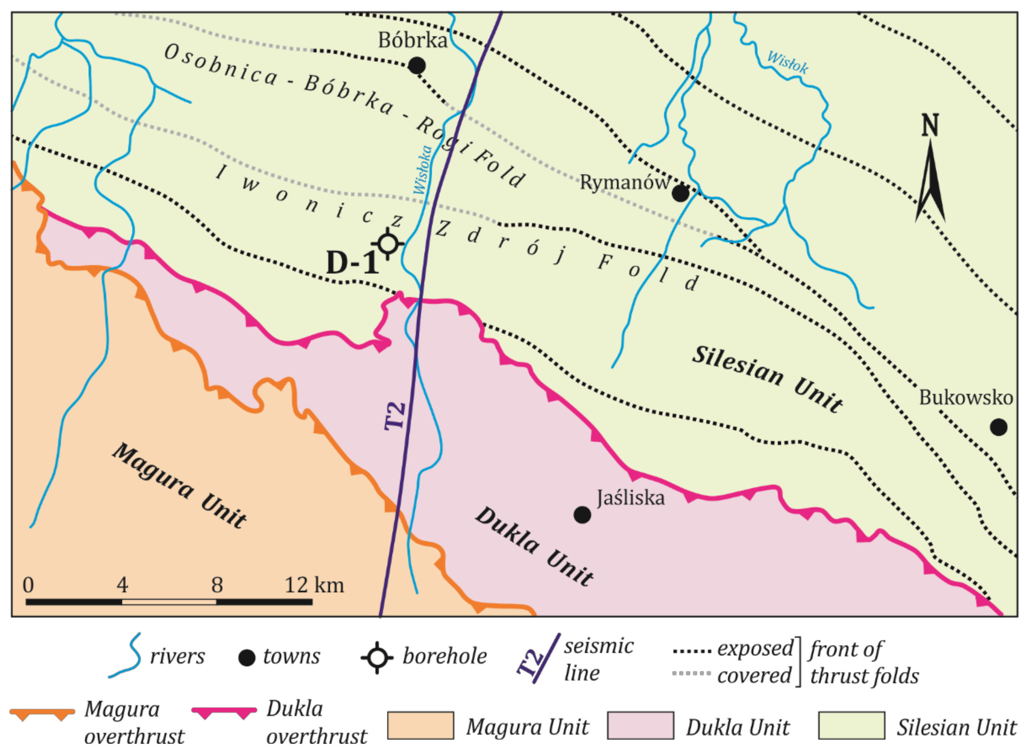
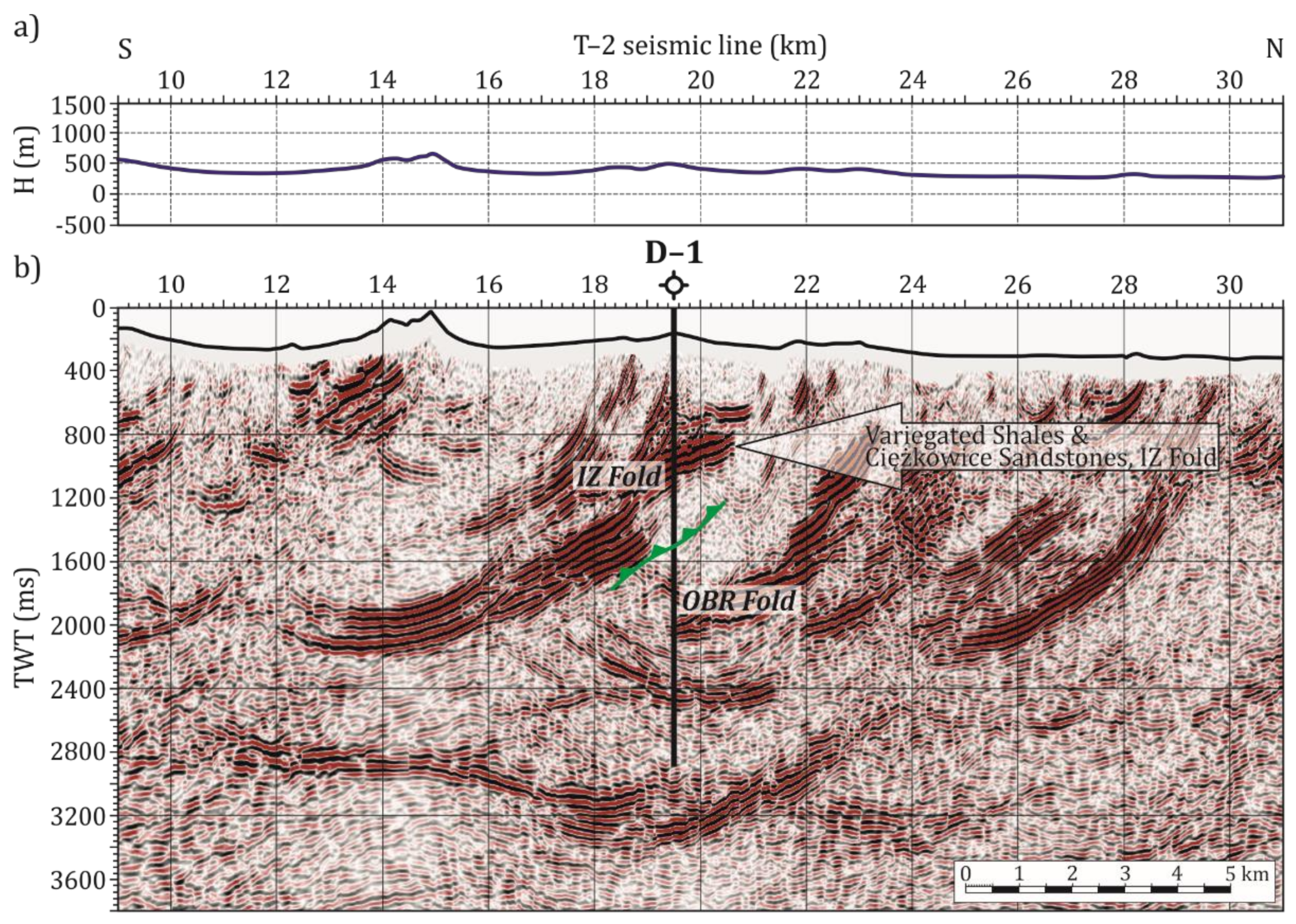
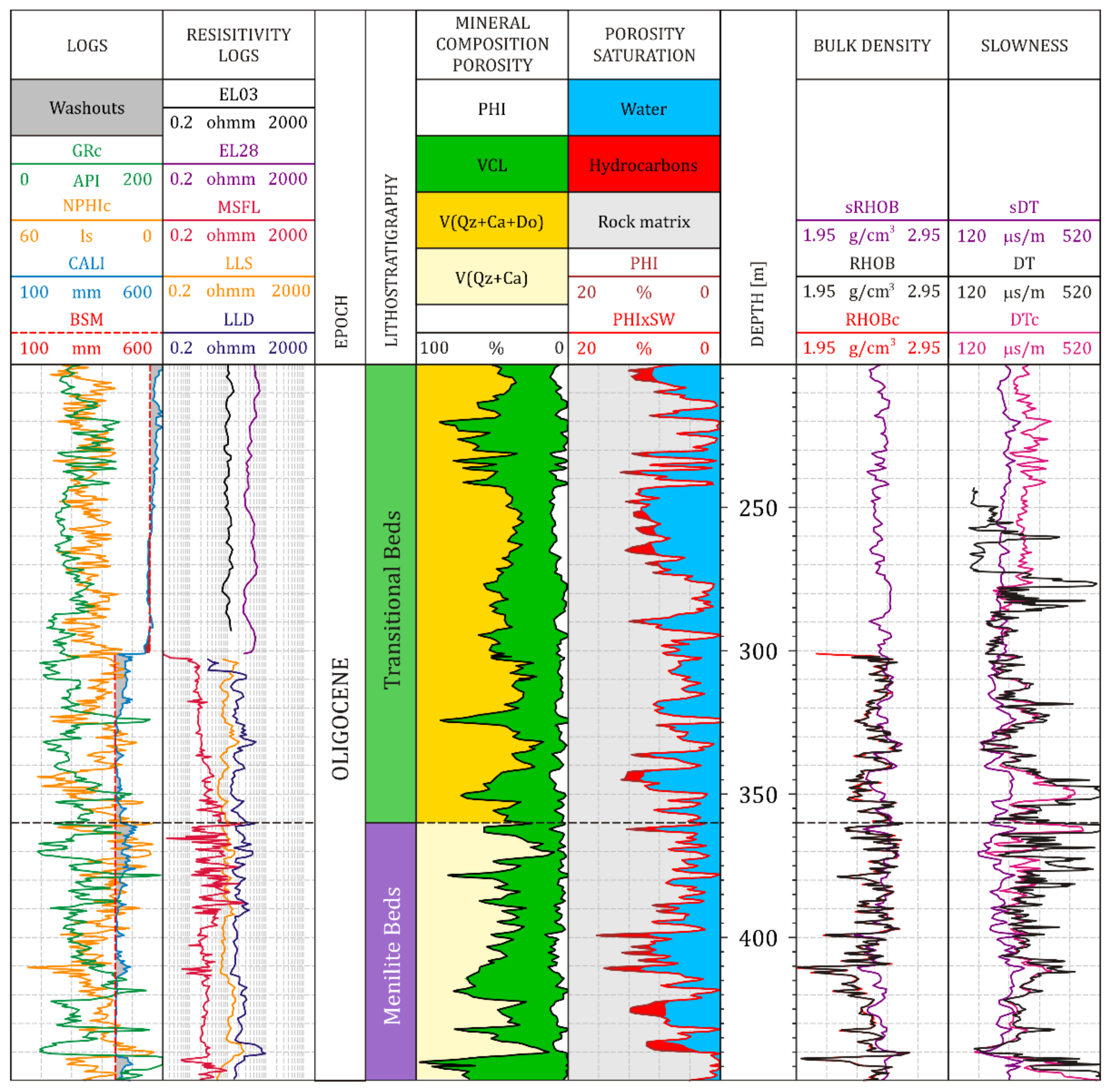
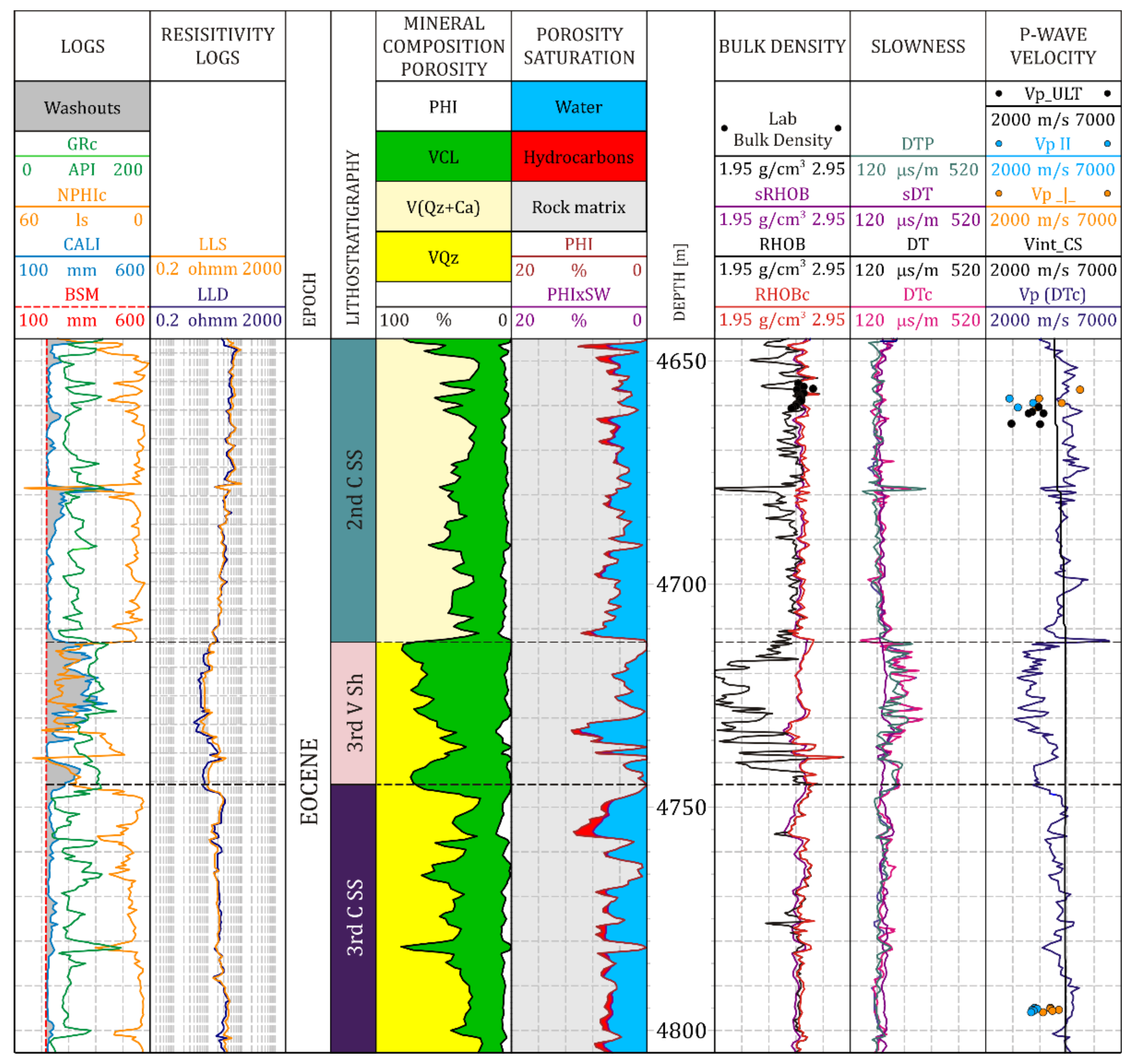
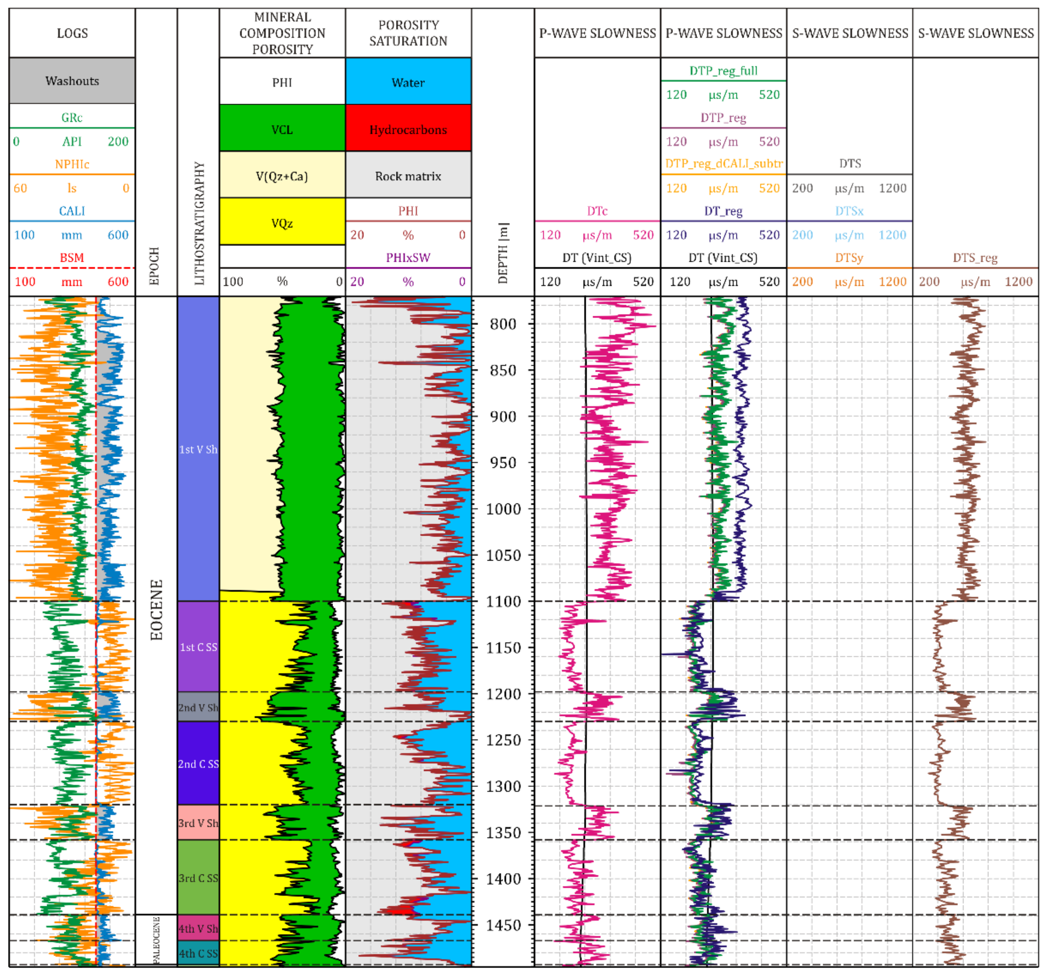
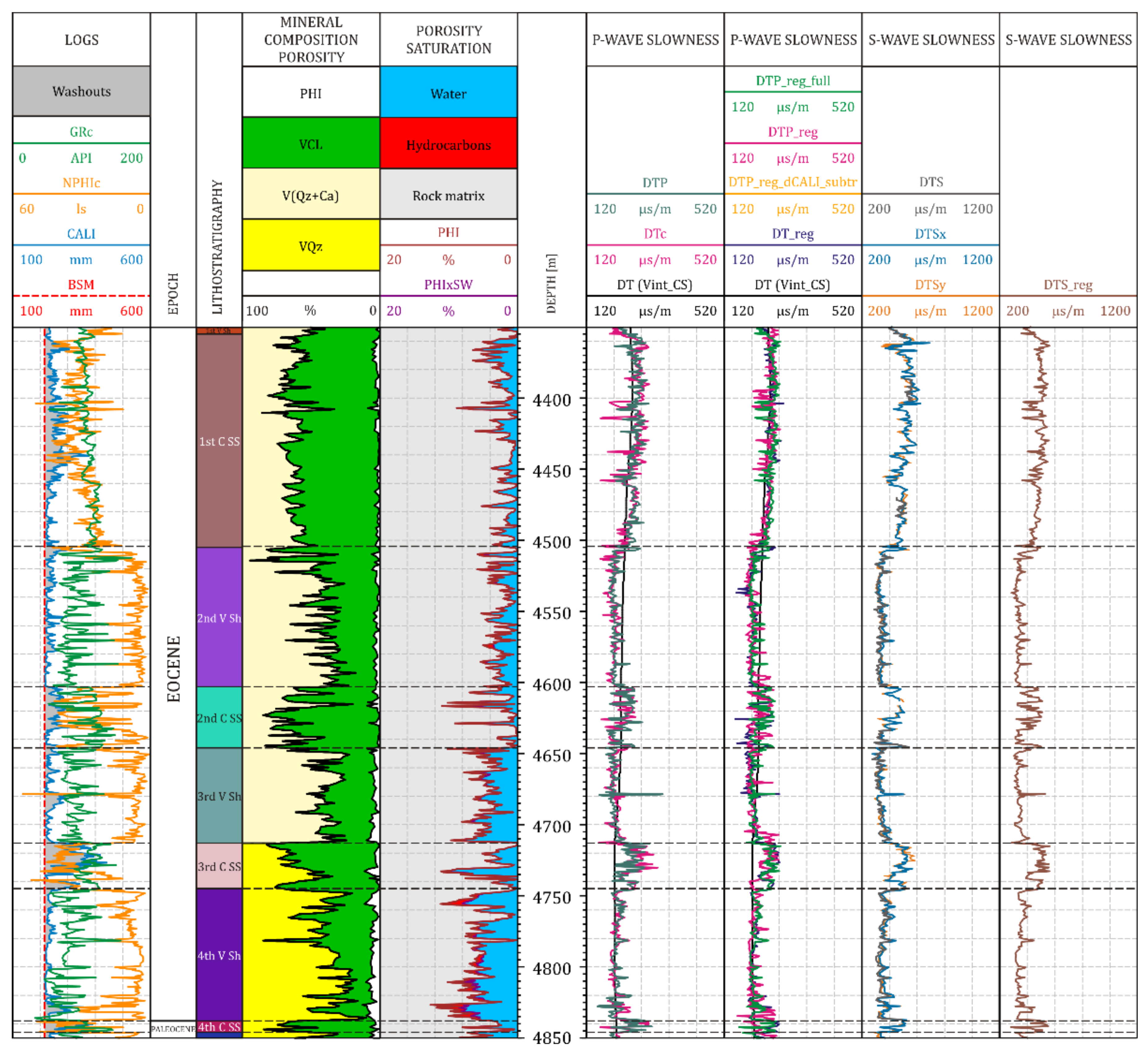
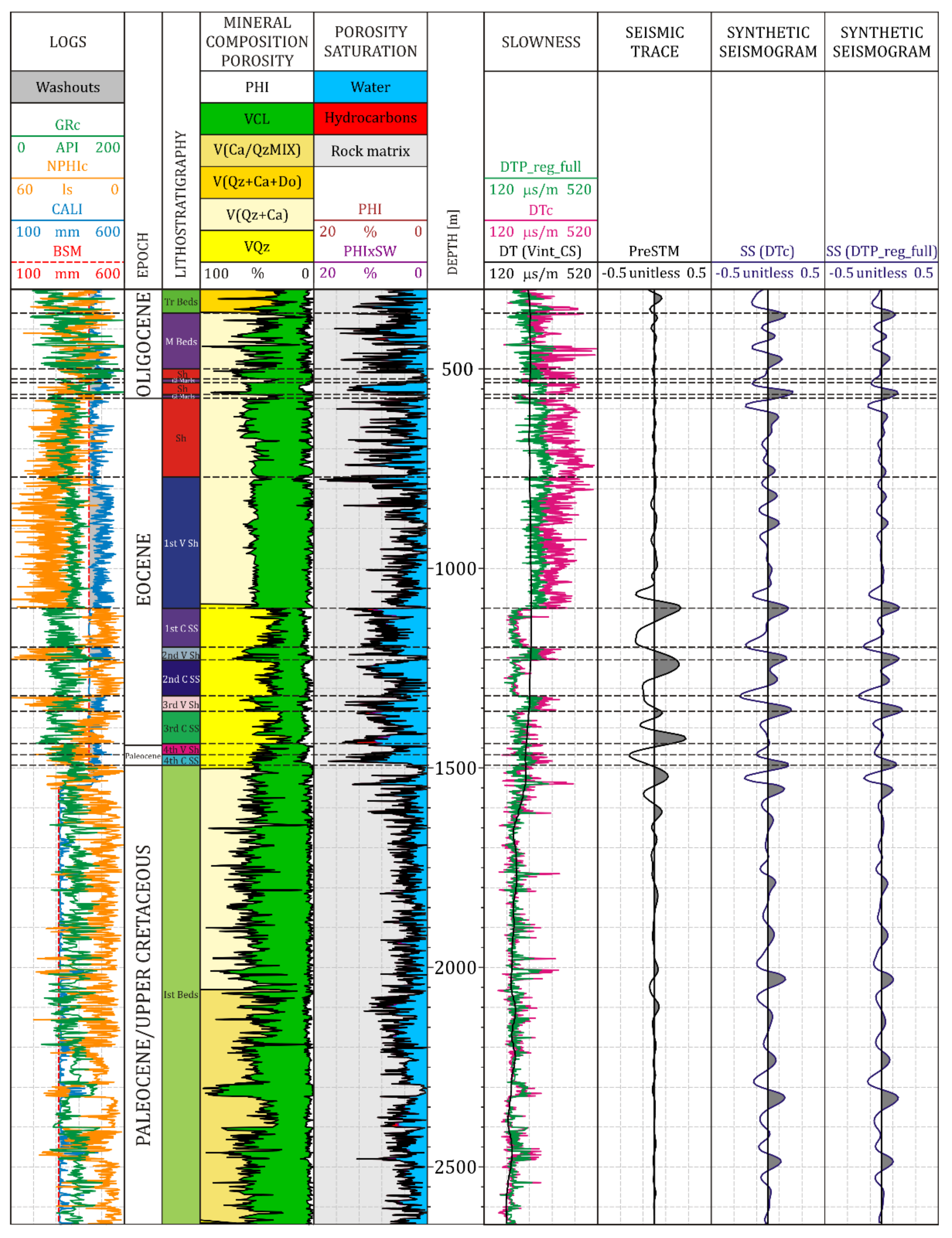
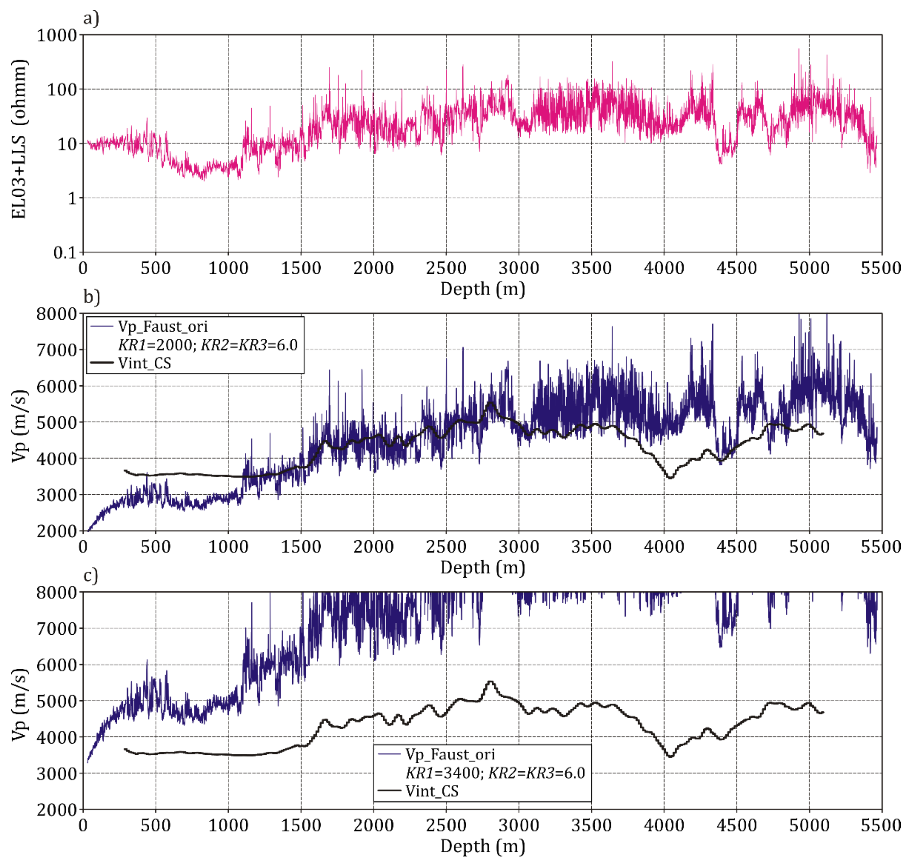
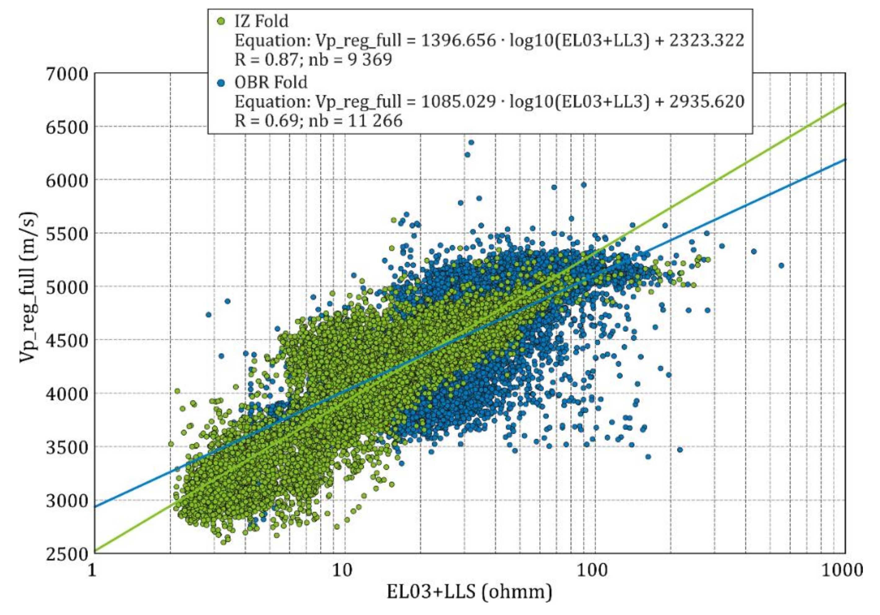
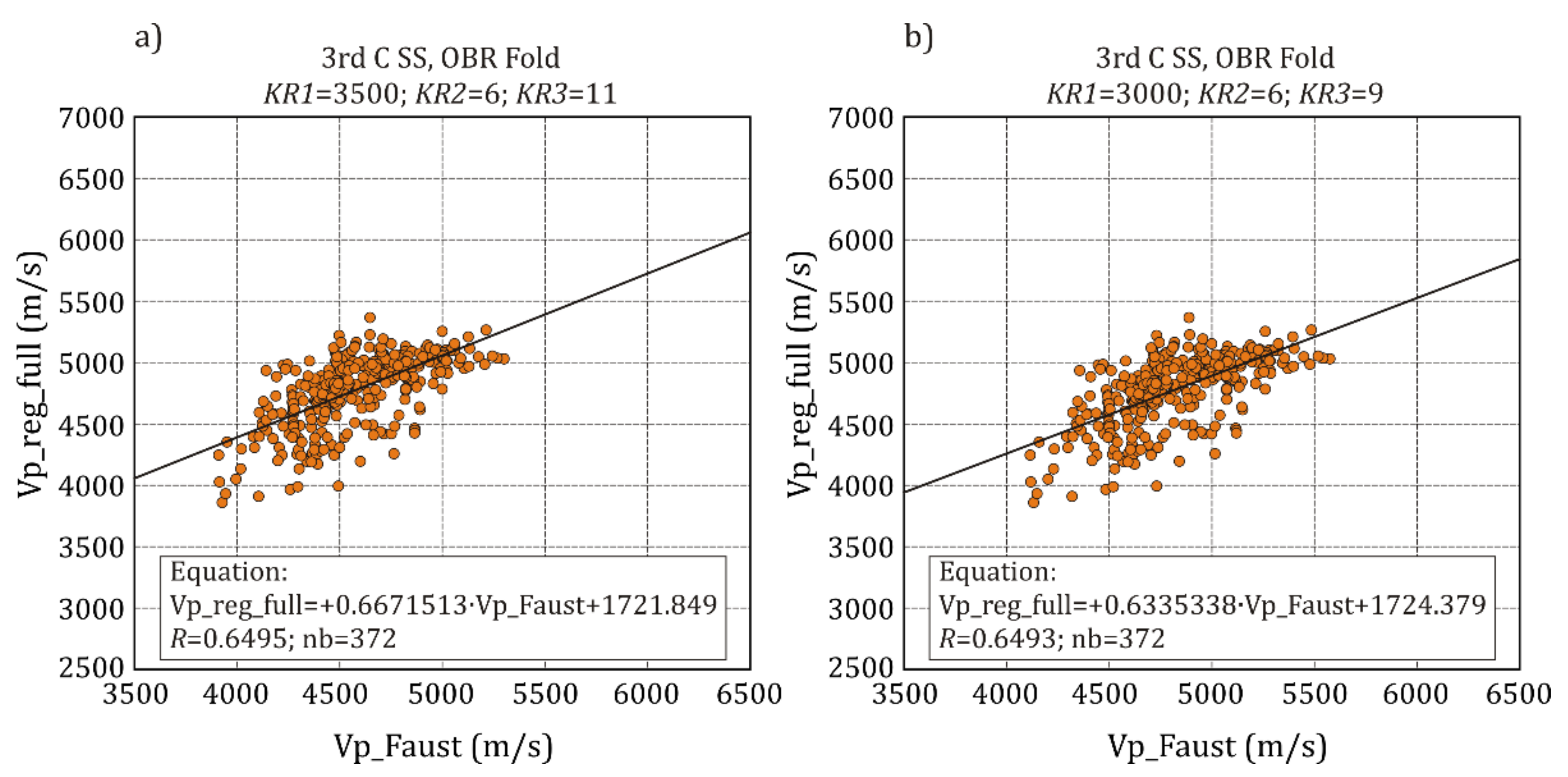
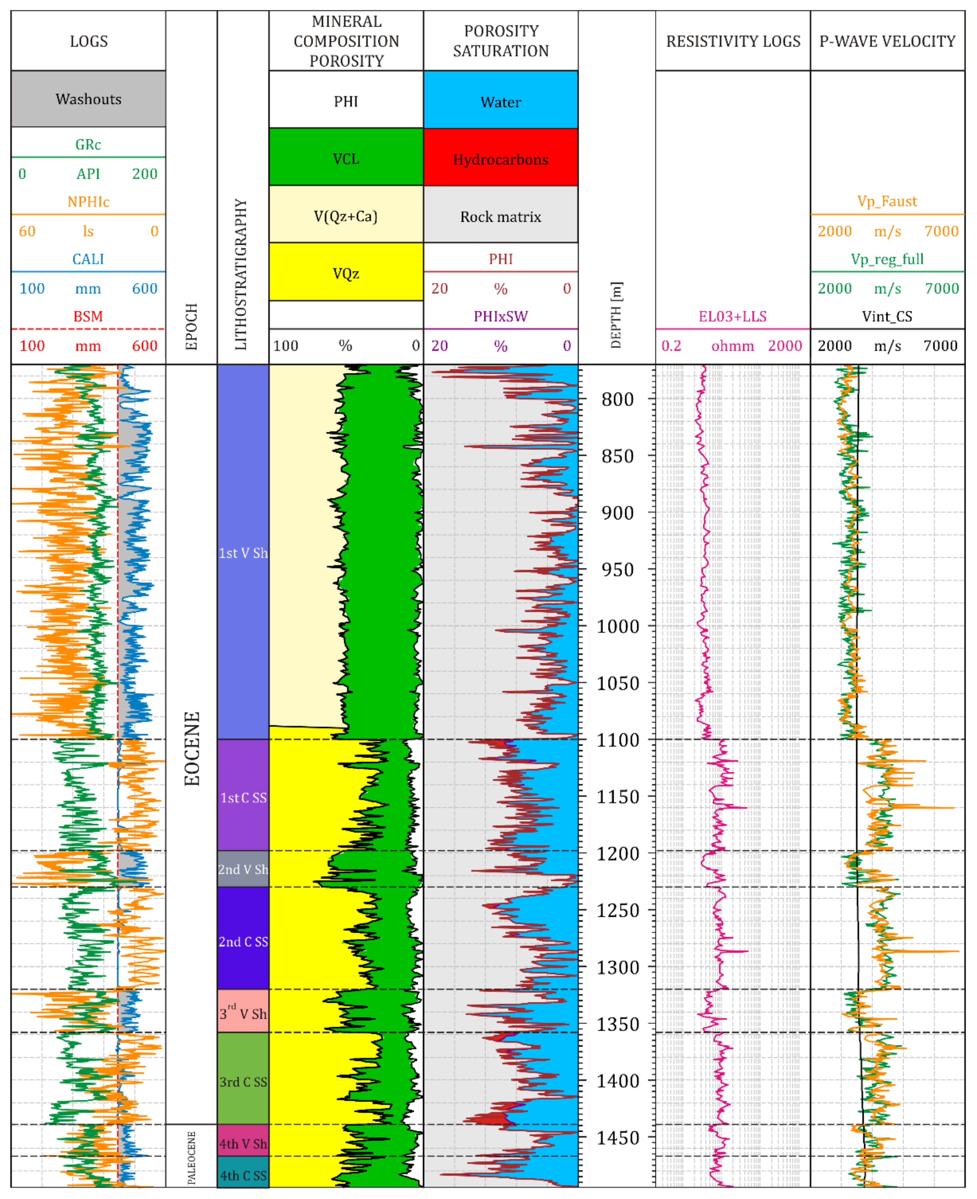
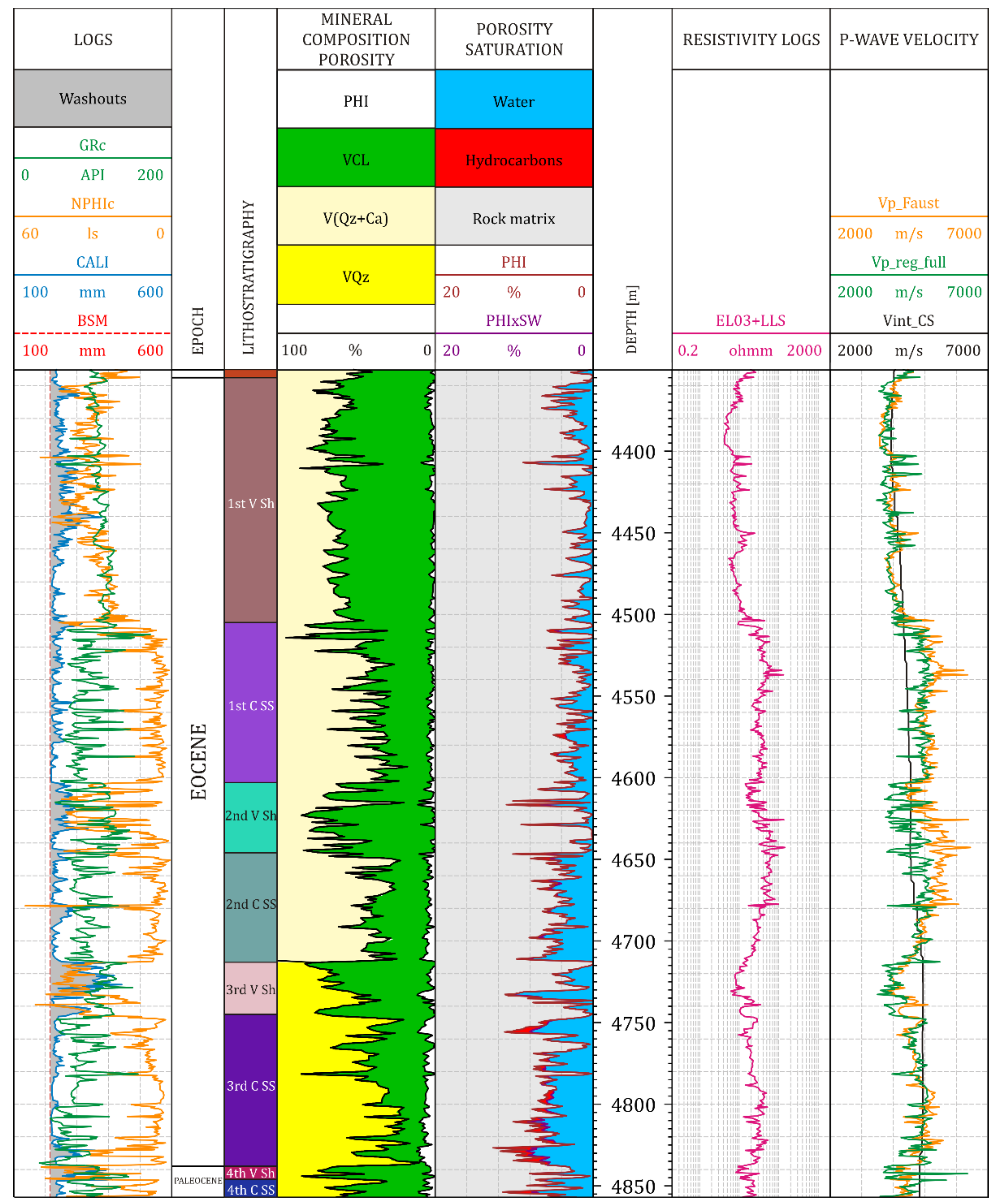
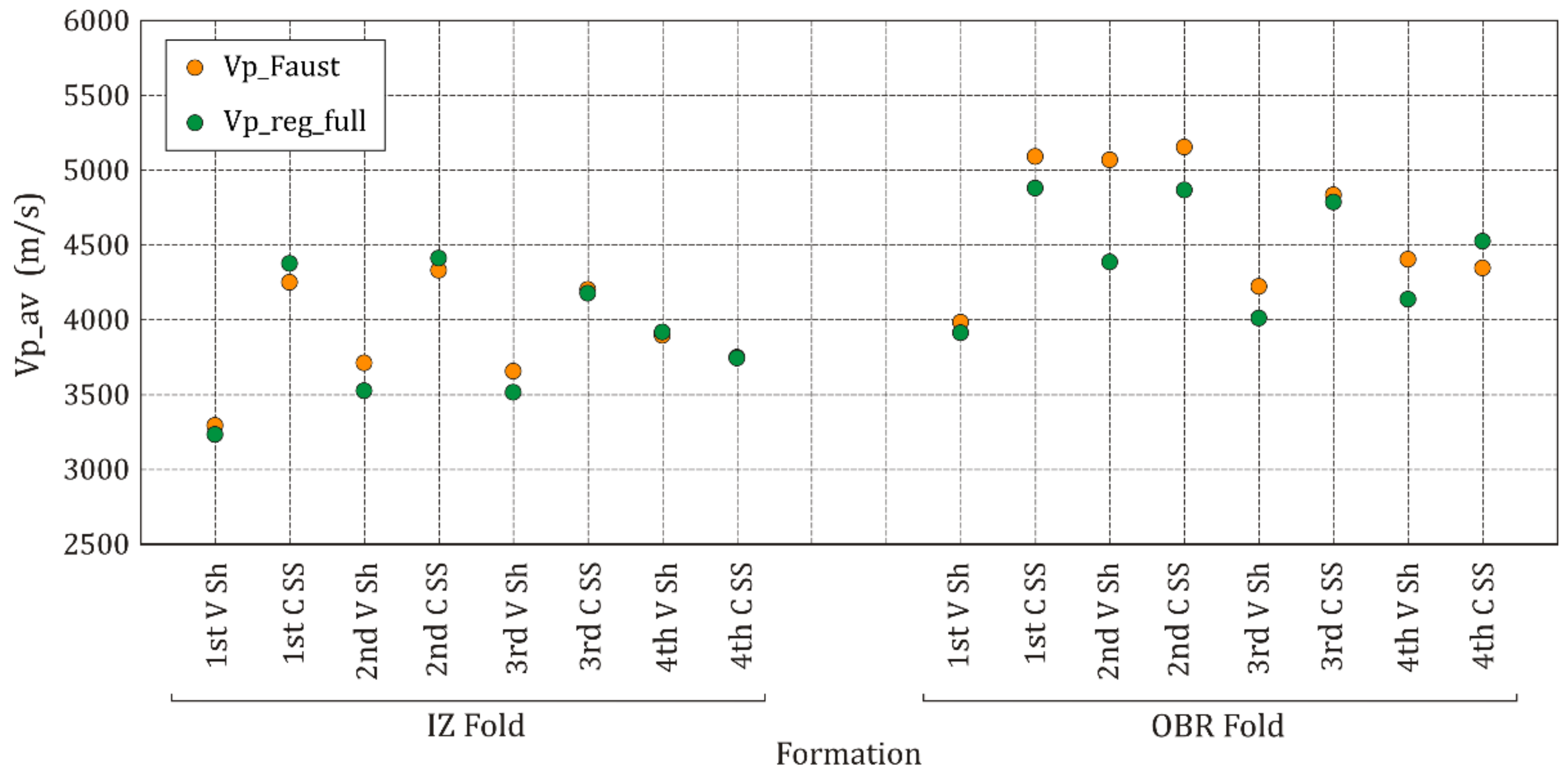
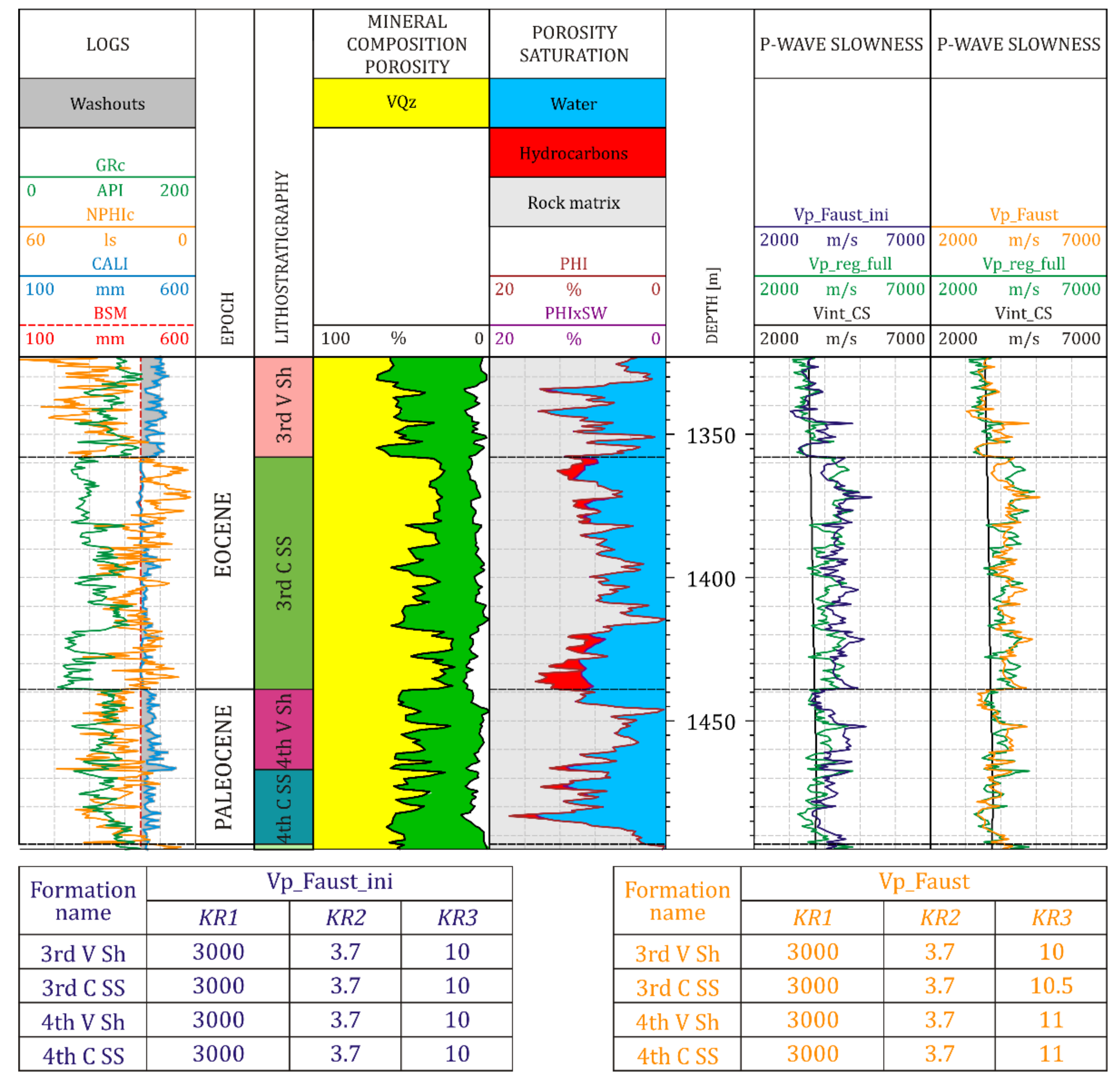
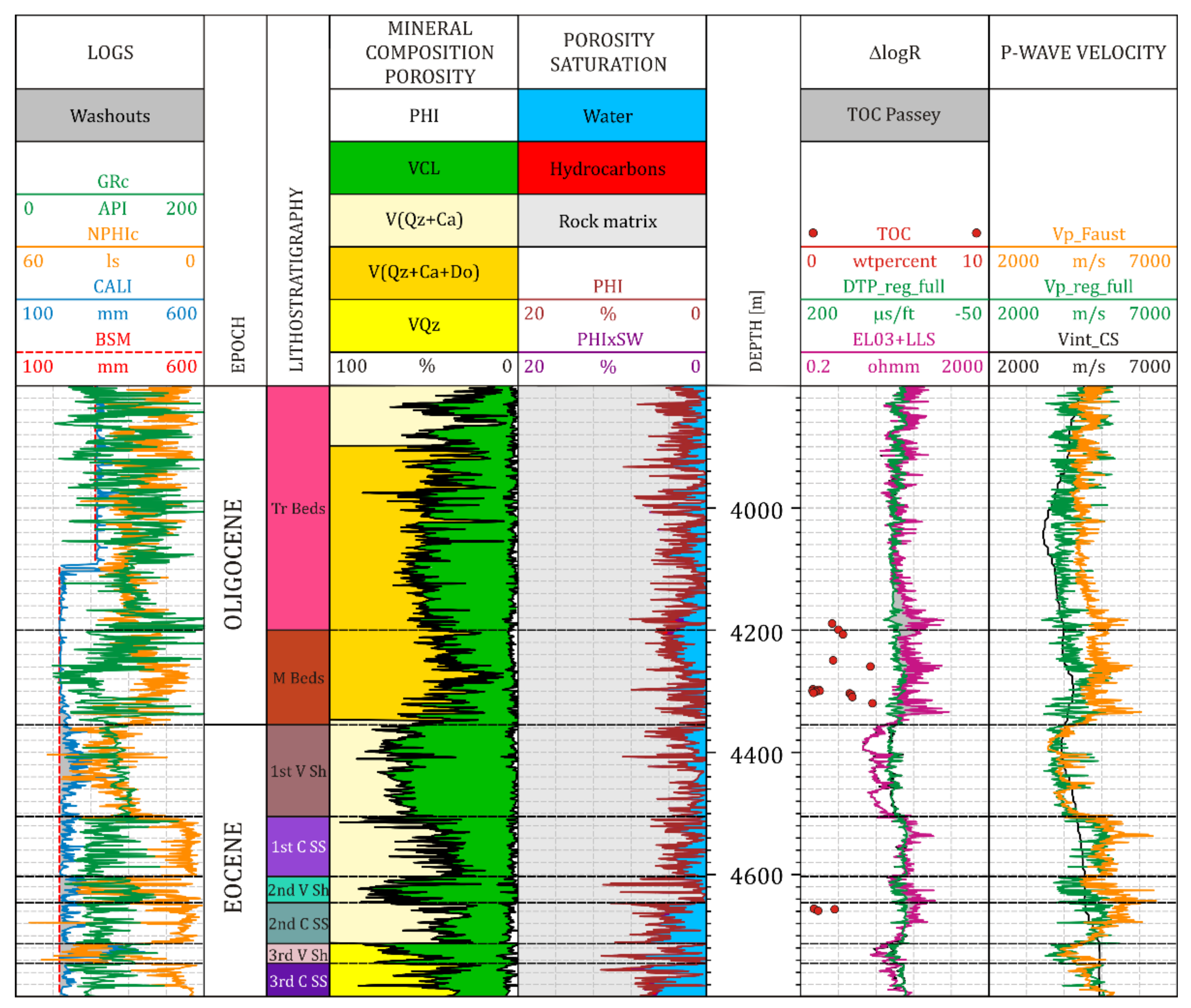