
Real-Time Load Variability Control Using Energy Storage System for Demand-Side Management in South Korea


Abstract
:1. Introduction
2. Conventional ESS Control for DSM
2.1. TOU Tariff Structure
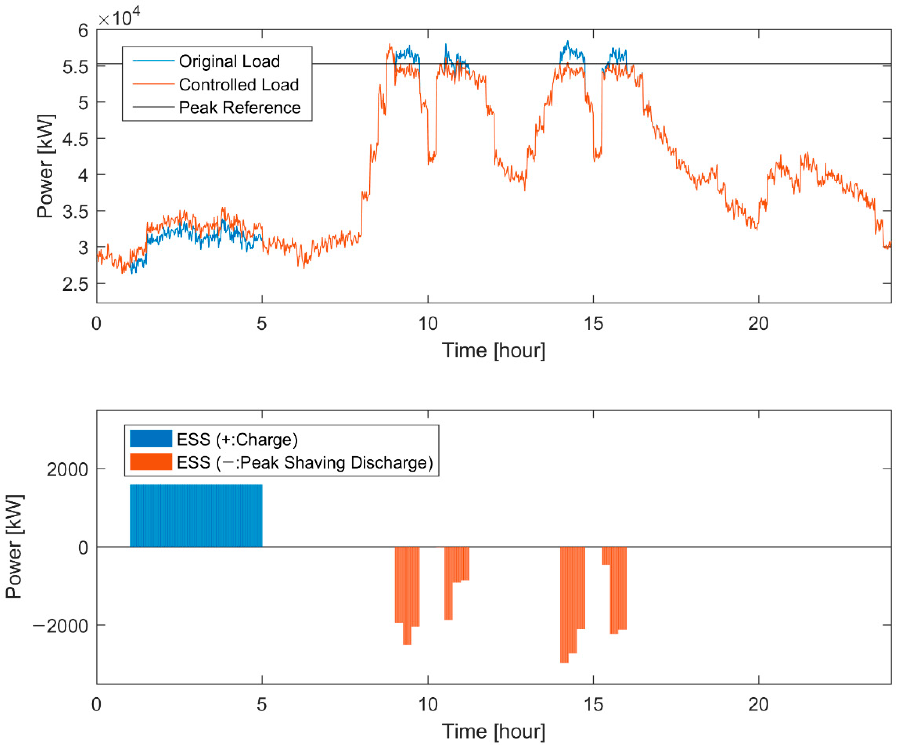
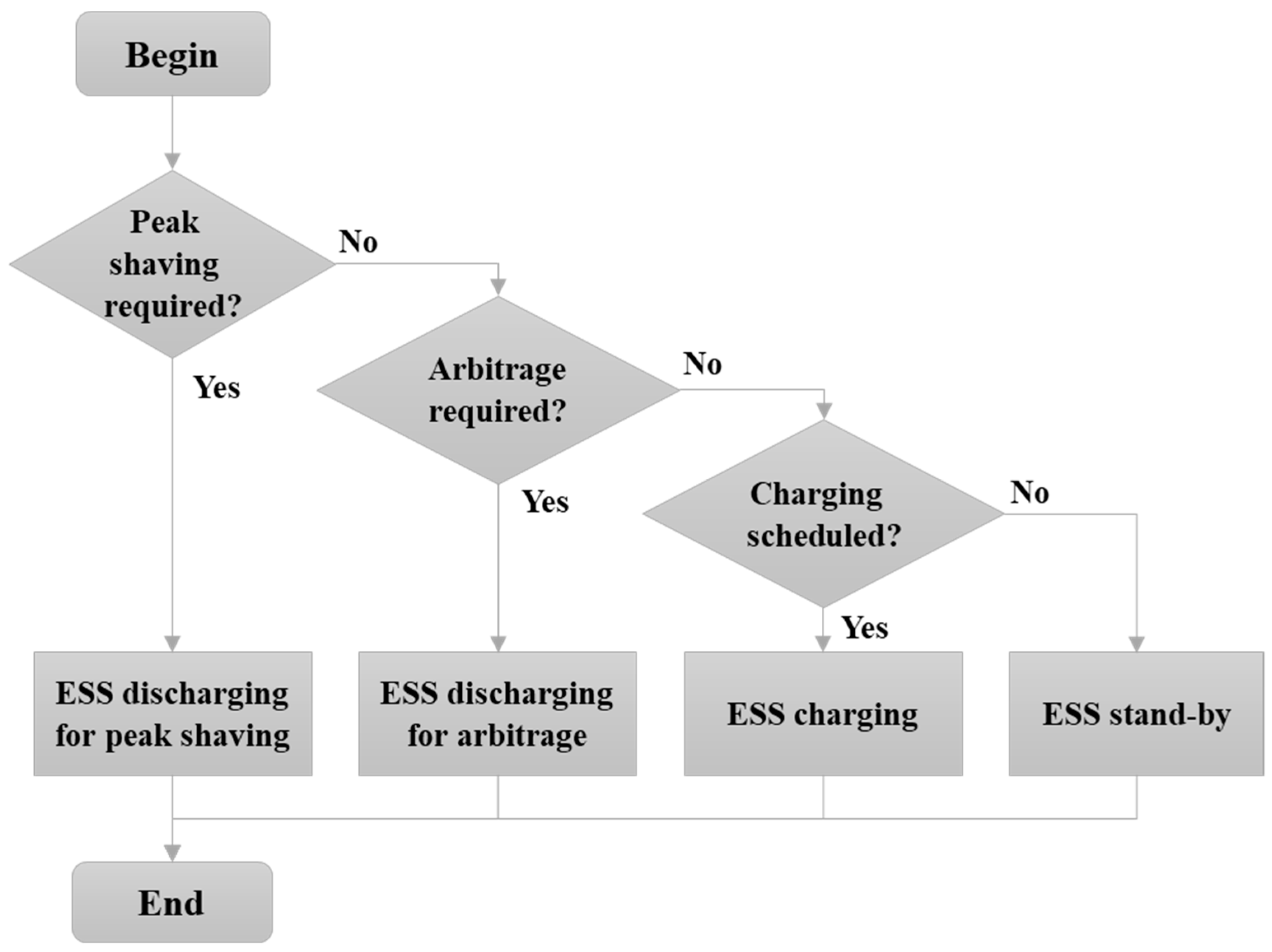
2.2. Peak Shaving and Arbitrage
3. Proposed ESS Operation for DSM
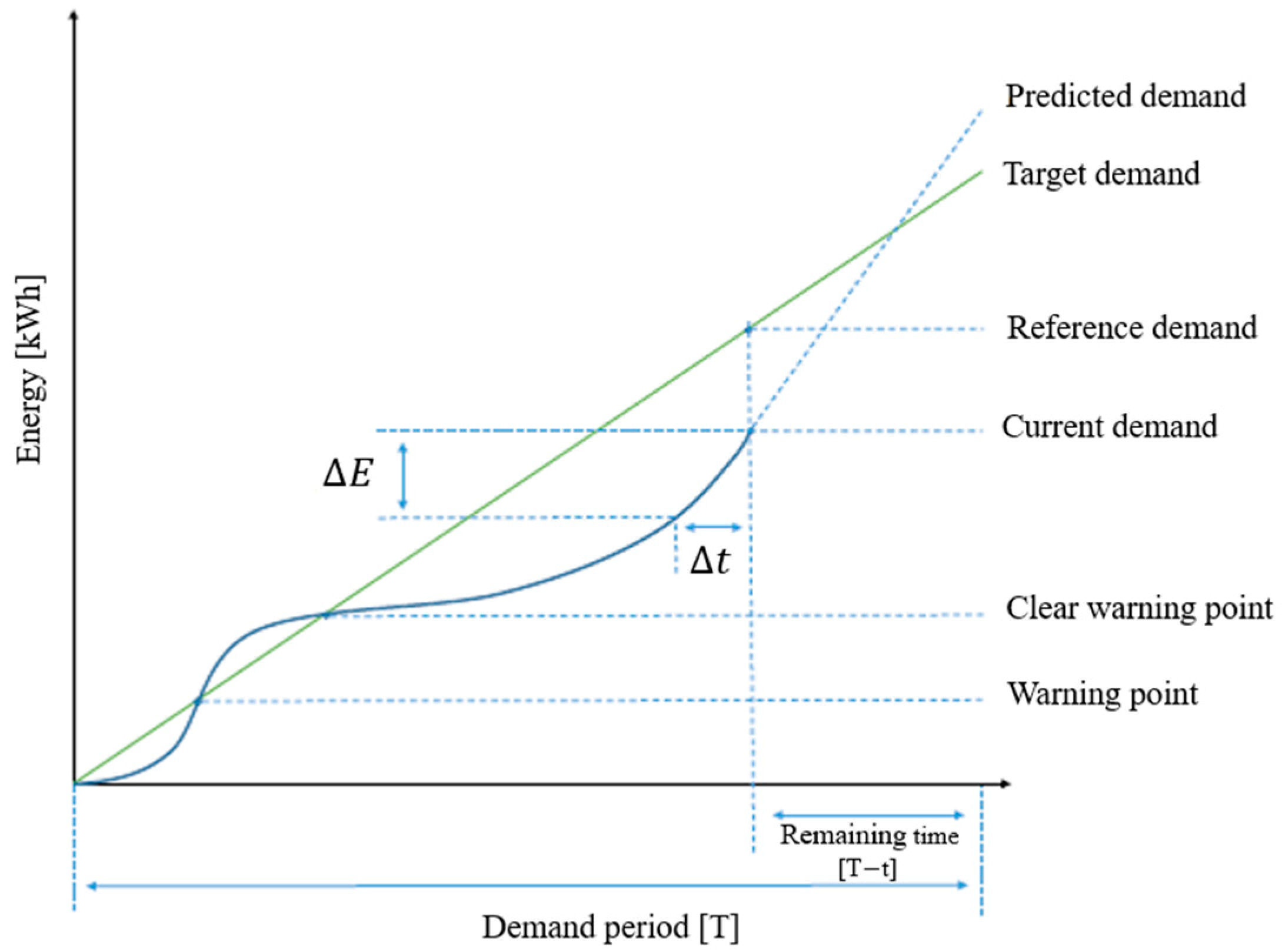
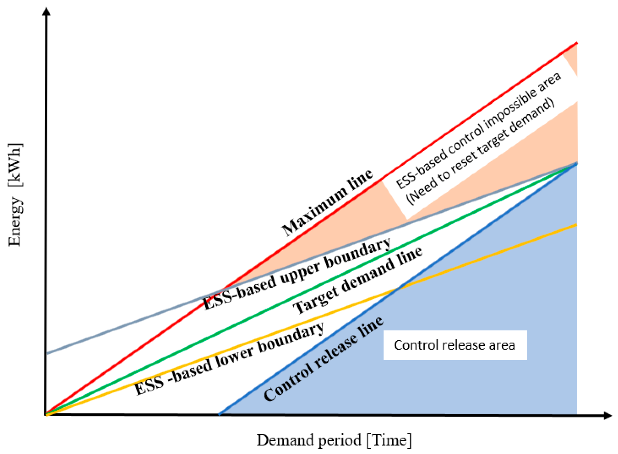
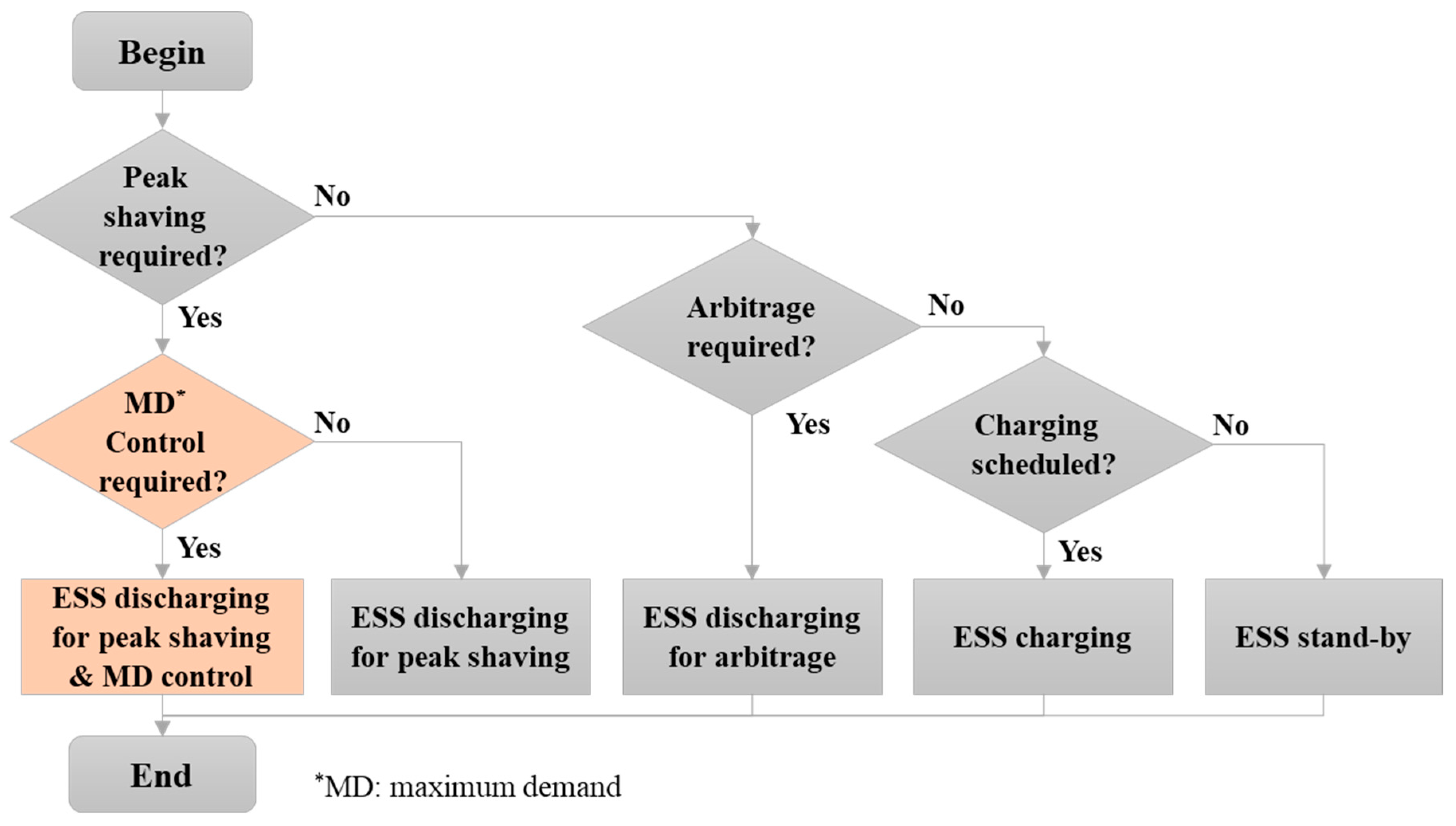
3.1. ESS-Based Maximum Demand Control
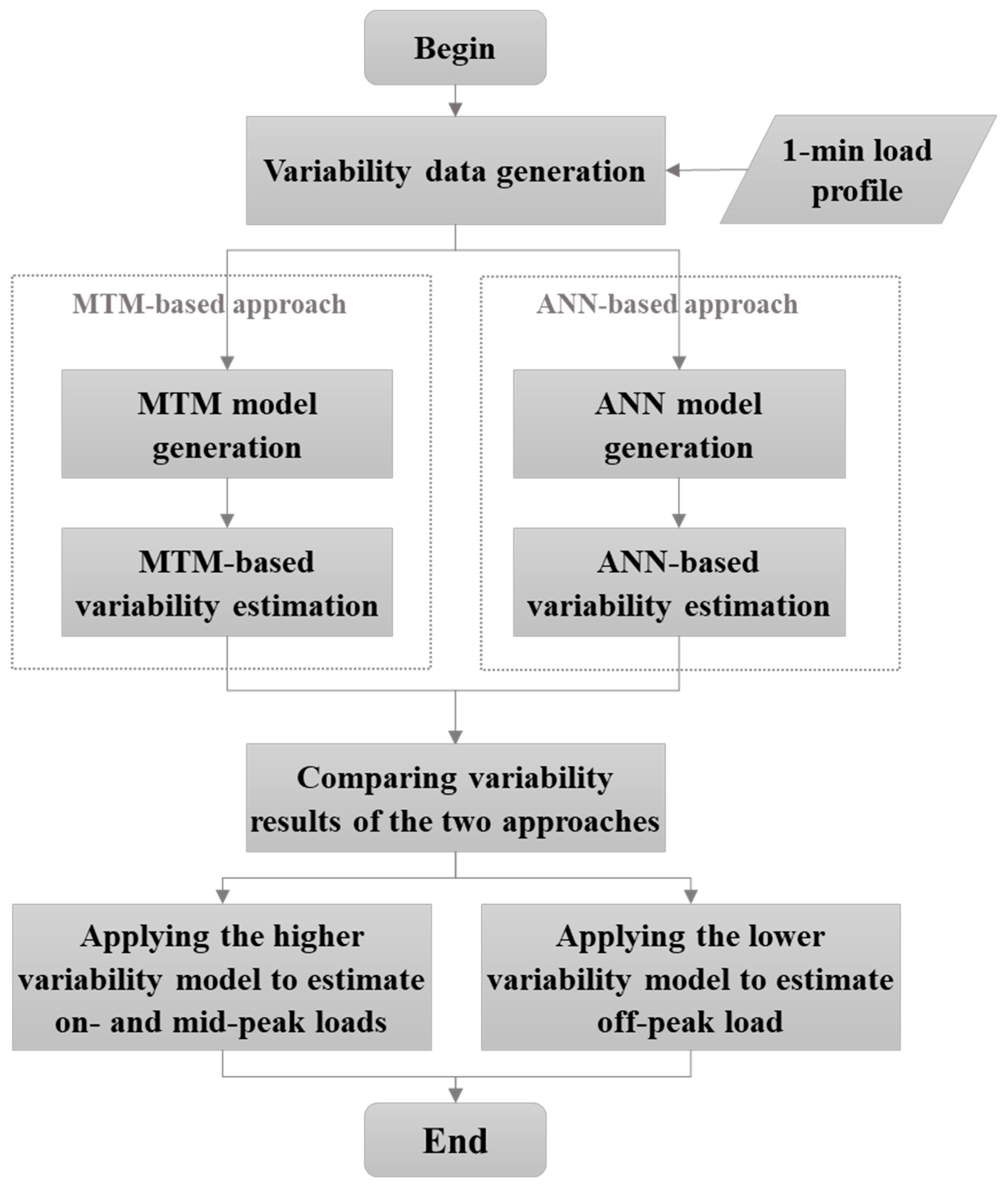
3.2. Estimation of 1-Min Load Variations
3.2.1. MTM-Based Estimation
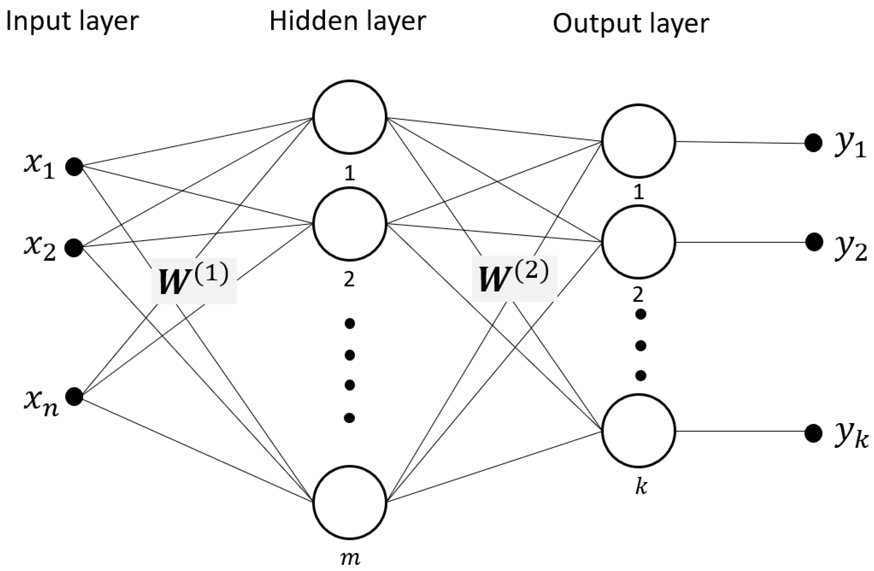
3.2.2. ANN-Based Estimation
3.2.3. Hybrid
3.3. ESS-Based DSM: A Proposal
- Step 1: Generating synthetic load profiles including minute-by-minute load fluctuations for an entire year using the proposed hybrid estimation model described in Section 3.2.3;
- Step 2: Calculating optimal capacity within the ESS for controlling maximum demand, as described in Section 3.1, based on the generated 1-min synthetic load profiles; and
- Step 3: Establishing a new peak reference for simultaneous peak shaving and maximum demand control.
4. Simulation
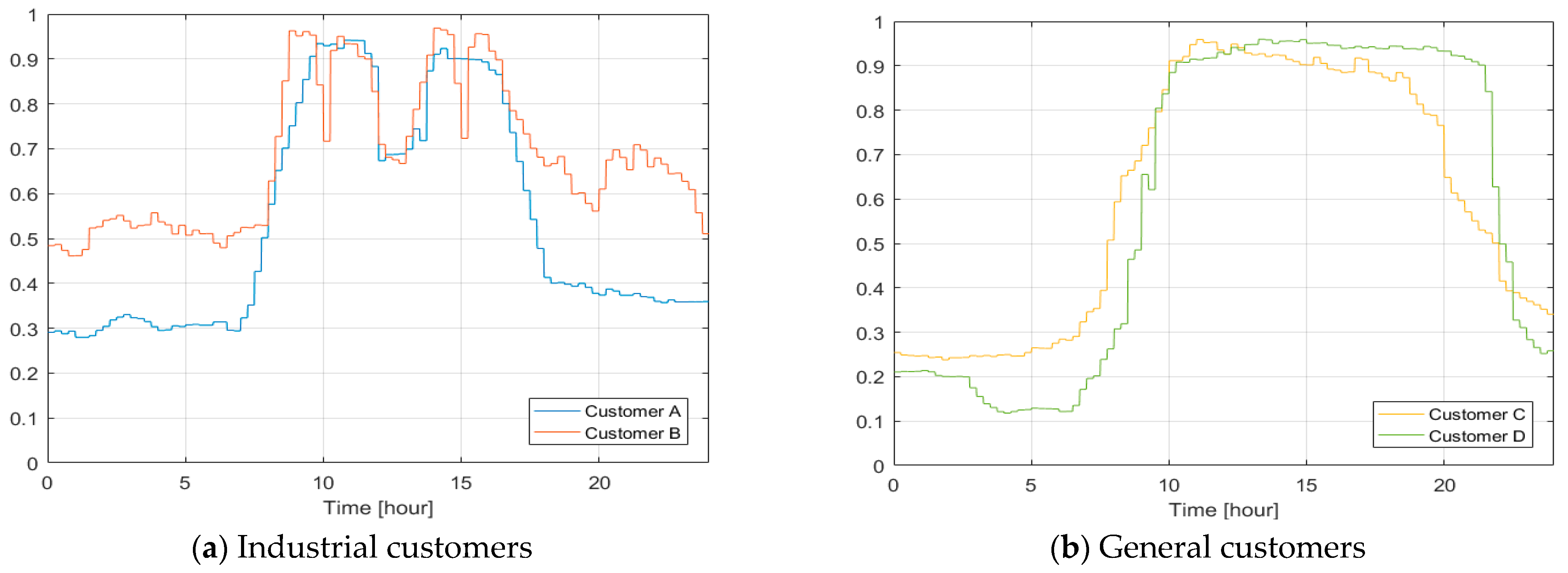
4.1. Data
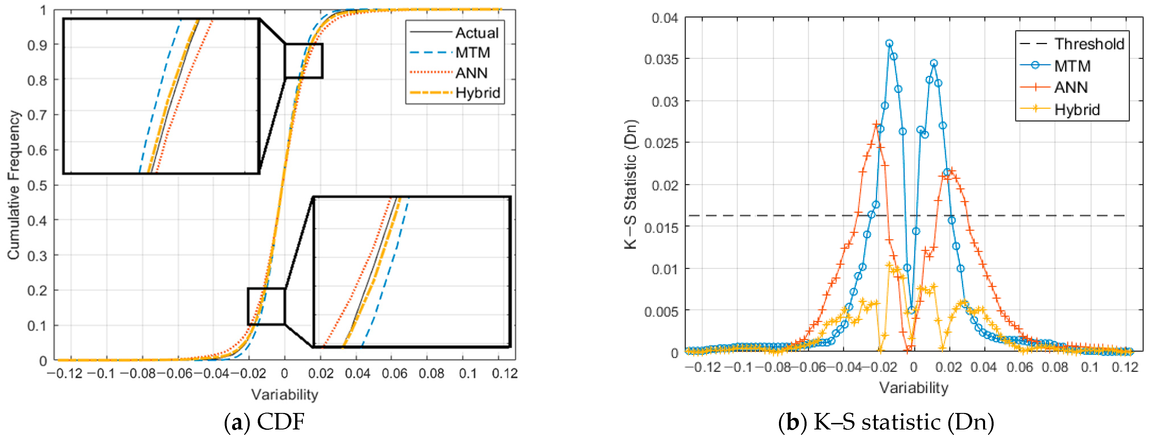
4.2. Verification of Estimating 1-Min Load Variations
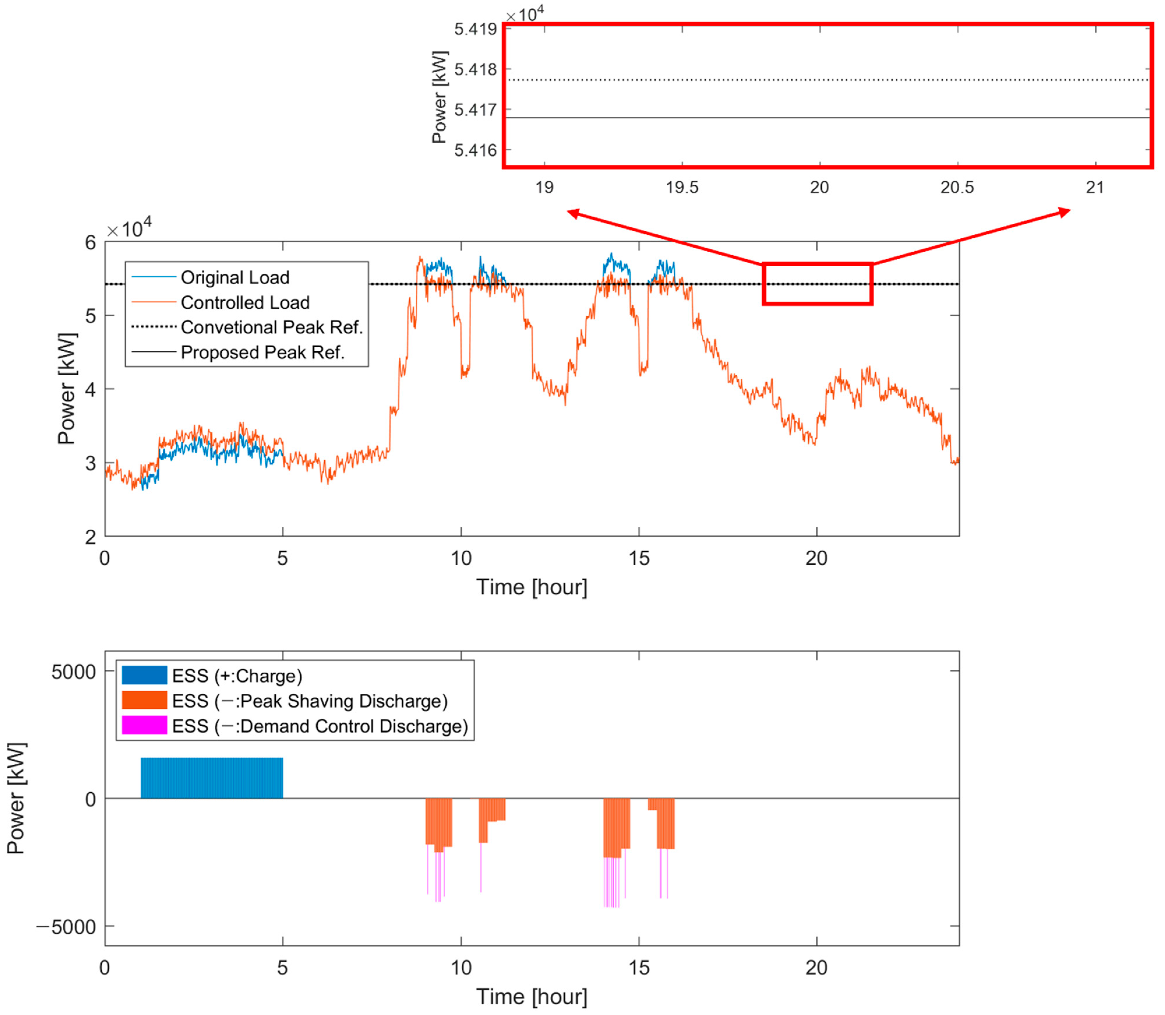
4.3. Result of the Simulation of the Proposed ESS-Based DSM
5. Conclusions
Author Contributions
Funding
Data Availability Statement
Conflicts of Interest
References
- Moslehi, K.; Kumar, R. A Reliability Perspective of the Smart Grid. IEEE Trans. Smart Grid 2010, 1, 57–64. [Google Scholar] [CrossRef]
- Kodaira, D.; Yu, B.; Jung, W.; Han, S. Optimized ESS Operation for Peak Shaving based on Probabilistic Load Prediction. In Proceedings of the 2018 IEEE Innovative Smart Grid Technologies-Asia (ISGT Asia), Singapore, 22–25 May 2018; pp. 1199–1203. [Google Scholar]
- Anjana, S.P.; Angel, T.S. Intelligent demand side management for residential users in a smart micro-grid. In Proceedings of the 2017 International Conference on Technological Advancements in Power and Energy (TAP Energy), Kollam, India, 21–23 December 2017; pp. 1–5. [Google Scholar]
- Kim, S.H.; Lee, G.; Shin, Y.J. Economical Energy Storage Systems Scheduling Based on Load Forecasting Using Deep Learning. In Proceedings of the 2019 IEEE International Conference on Big Data and Smart Computing (BigComp), Kyoto, Japan, 27 Feburary–2 March 2019; pp. 1–7. [Google Scholar]
- Korea Electric Power Corp. Electrical Supply Terms and Conditions. Available online: http://cyber.kepco.co.kr (accessed on 19 October 2020).
- Strbac, G. Demand side management: Benefits and challenges. Energy Policy 2008, 36, 4419–4426. [Google Scholar] [CrossRef]
- Gelazanskas, L.; Gamage, K.A.A. Demand side management in smart grid: A review and proposals for future direction. Sustain. Cities Soc. 2014, 11, 20–30. [Google Scholar] [CrossRef]
- Dharani, R.; Balasubramonian, M.; Babu, T.S.; Nastasi, B. Load Shifting and Peak Clipping for Reducing Energy Consumption in an Indian University Campus. Energies 2021, 14, 558. [Google Scholar] [CrossRef]
- Warren, P. A review of demand-side management policy in the UK. Renew. Sustain. Energy Rev. 2014, 29, 941–951. [Google Scholar] [CrossRef]
- Kang, B.O.; Lee, M.; Kim, Y.; Jung, J. Economic analysis of a customer-installed energy storage system for both self-saving operation and demand response program participation in South Korea. Renew. Sustain. Energy Rev. 2018, 94, 69–83. [Google Scholar] [CrossRef]
- Leadbetter, J.; Swan, L. Battery storage system for residential electricity peak demand shaving. Energy Build 2012, 55, 685–692. [Google Scholar] [CrossRef]
- Martins, R.; Hesse, H.C.; Jungbauer, J.; Vorbuchner, T.; Musilek, P. Optimal Component Sizing for Peak Shaving in Battery Energy Storage System for Industrial Applications. Energies 2018, 11, 2048. [Google Scholar] [CrossRef] [Green Version]
- De Salis, R.T.; Clarke, A.; Wang, Z.; Moyne, J.; Tilbury, D.M. Energy storage control for peak shaving in a single building 2014. In Proceedings of the IEEE PES General Meeting | Conference & Exposition, National Harbor, MD, USA, 27–31 July 2014; pp. 1–5. [Google Scholar]
- Kim, S.; Kim, J.; Cho, K.; Byeon, G. Optimal operation control for multiple BESSs of a large-scale customer under time-based pricing. IEEE Trans. Power Syst. 2018, 33, 803–816. [Google Scholar] [CrossRef]
- Kodaira, D.; Jung, W.; Han, S. Optimal Energy Storage System Operation for Peak Reduction in a Distribution Network Using a Prediction Interval. IEEE Trans. Smart Grid 2020, 11, 2208–2217. [Google Scholar] [CrossRef]
- Yoon, Y.; Kim, Y.-H. Charge Scheduling of an Energy Storage System under Time-of-Use Pricing and a Demand Charge. Sci. World J. 2014, 2014, 937329. [Google Scholar] [CrossRef] [PubMed] [Green Version]
- Lee, W.; Kang, B.O.; Jung, J. Development of energy storage system scheduling algorithm for simultaneous self-consumption and demand response program participation in South Korea. Energy 2018, 161, 963–973. [Google Scholar] [CrossRef]
- Jeong, H.C.; Jung, J.; Kang, B.O. Development of Operational Strategies of Energy Storage System Using Classification of Customer Load Profiles under Time-of-Use Tariffs in South Korea. Energies 2020, 13, 1723. [Google Scholar] [CrossRef] [Green Version]
- Parra, D.; Gillott, M.; Norman, S.A.; Walker, G.S. Optimum community energy storage system for PV energy time-shift. Appl. Energy 2013, 137, 576–587. [Google Scholar] [CrossRef]
- Beaudin, M.; Zareipour, H.; Schellenberglabe, A.; Rosehart, W. Energy storage for mitigating the variability of renewable electricity sources: An updated review. Energy Sustain. Dev. 2010, 14, 302–314. [Google Scholar] [CrossRef]
- Hussain, S.; Ahmed, M.A.; Kim, Y.-C. Efficient Power Management Algorithm Based on Fuzzy Logic Inference for Electric Vehicles Parking Lot. IEEE Access 2019, 7, 65467–65485. [Google Scholar] [CrossRef]
- Hussain, S.; Ahmed, M.A.; Lee, K.-B.; Kim, Y.-C. Fuzzy Logic Weight Based Charging Scheme for Optimal Distribution of Charging Power among Electric Vehicles in a Parking Lot. Energies 2020, 13, 3119. [Google Scholar] [CrossRef]
- Hussain, S.; Lee, K.-B.; Ahmed, M.A.; Hayes, B.; Kim, Y.-C. Two-Stage Fuzzy Logic Inference Algorithm for Maximizing the Quality of Performance under the Operational Constraints of Power Grid in Electric Vehicle Parking Lots. Energies 2020, 13, 4634. [Google Scholar] [CrossRef]
- Ngoko, B.; Sugihara, H.; Funaki, T. Synthetic generation of high temporal resolution solar radiation data using Markov models. Sol. Energy 2014, 103, 160–170. [Google Scholar] [CrossRef]
- Kang, B.O.; Tam, K.-S. A new characterization and classification method for daily sky conditions based on ground-based solar irradiance measurement data. Sol. Energy 2013, 94, 102–118. [Google Scholar] [CrossRef]
- Pillai, G.G.; Putrus, G.A.; Pearsall, N.M. Generation of synthetic benchmark electrical load profiles using publicly available load and weather data. Int. J. Electr. Power 2014, 61, 1–10. [Google Scholar] [CrossRef] [Green Version]
- Ekonomou, L.; Oikonomou, D. Application and comparison of several artificial neural networks for forecasting the Hellenic daily electricity demand load. In Proceedings of the 7th WSEAS International Conference on Artificial Intelligence, Knowledge Engineering and Data Bases, Cairo, Egypt, 29–31 December 2008; pp. 67–71. [Google Scholar]
- Chua, K.H.; Lim, Y.S.; Morris, S. A novel fuzzy control algorithm for reducing the peak demands using energy storage system. Energy 2017, 122, 265–273. [Google Scholar] [CrossRef]
- Castellanos, J.D.A.; Rajan, H.D.V.; Rohde, A.K.; Denhof, D.; Freitag, M. Design and simulation of a control algorithm for peak-load shaving using vehicle to grid technology. SN Appl. Sci. 2019, 1, 951. [Google Scholar] [CrossRef] [Green Version]
- Jorge, H.; Martins, A.; Gomes, A. Maximum demand control: A survey and comparative evaluation of different methods. IEEE Trans. Power Syst. 1993, 8, 1013–1019. [Google Scholar] [CrossRef]
- Hoffman, A.J. Peak demand control in commercial buildings with target peak adjustment based on load forecasting. In Proceedings of the 1998 IEEE International Conference on Control Applications (Cat. No. 98CH36104), Trieste, Italy, 4 September 1998; Volume 2, pp. 1292–1296. [Google Scholar]
- Han, K.B.; Jeong, H.C.; Kang, B.O. Maximum Demand Control Method using Customer-Installed Energy Storage System. In Proceedings of the 2018 Korean Institute of Electrical Engineers Summer Conference, Pyeongchang, Korea, 11–13 July 2018; Volume 7, pp. 31–32. [Google Scholar]
- Sahin, A.D.; Sen, Z. First-order Markov chain approach to wind speed modeling. J. Wind Engng. Ind. Aerodyn. 2001, 89, 263–269. [Google Scholar] [CrossRef]
- Ryu, S.; Noh, J.; Kim, H. Deep Neural Network Based Demand Side Short Term Load Forecasting. Energies 2017, 10, 3. [Google Scholar] [CrossRef]
- Kong, J.; Jufri, F.H.; Kang, B.O.; Jung, J. Development of ESS SchedulingAlgorithm to Maximize the Potential Profitability of PV Generation Supplier in South Korea. J. Electr. Eng. Technol. 2018, 13, 2227–2235. [Google Scholar]
- Riedmiller, M.; Braun, H. A direct adaptive method for faster backpropagation learning: The RPROP algorithm. In Proceedings of the IEEE International Conference on Neural Networks, San Francisco, CA, USA, 28 Mrach–1 April 1993; pp. 586–591. [Google Scholar]
- Igel, C.; Hüsken, M. Improving the Rprop Learning Algorithm. In Proceedings of the Second International ICSC Symposium on Neural Computation (NC 2000), Berlin, Germany, 23–26 May 2000. [Google Scholar]
- Espinar, B.; Ramírez, L.; Drews, A.; Beyer, H.G.; Zarzalejo, L.F.; Polo, J.; Martín, L. Analysis of different comparison parameters applied to solar radiation data from satellite and German radiometric stations. Sol. Energy 2009, 83, 118–125. [Google Scholar] [CrossRef]
- Massey, F.J. The Kolmogorov-Smirnov test for goodness of fit. J. Am. Stat. Assoc. 1951, 46, 68–78. [Google Scholar] [CrossRef]


| Classification | Spring, Summer, and Fall (1 March–31 October) | Winter (1 November–28 February) |
|---|---|---|
| Off-peak | 23:00–09:00 | 23:00–09:00 |
| Mid-peak | 09:00–10:00 12:00–13:00 17:00–23:00 | 09:00–10:00 12:00–17:00 20:00–22:00 |
| On-peak | 10:00–12:00 13:00–17:00 | 10:00–12:00 17:00–20:00 22:00–23:00 |
| Class | |||||
|---|---|---|---|---|---|
| Period | Summer | Spring & Fall | Winter | ||
| Industrial service (B) High-voltage (B), Option II | 7380 | Off-peak load | 56.2 | 56.2 | 63.2 |
| Mid-peak load | 108.5 | 78.5 | 108.5 | ||
| On-peak load | 189.7 | 108.8 | 164.7 | ||
| General service (B) High-voltage (A), Option II | 8320 | Off-peak load | 56.1 | 56.1 | 63.1 |
| Mid-peak load | 109.0 | 78.6 | 109.2 | ||
| On-peak load | 191.1 | 109.3 | 166.7 | ||
| Variables | Information | |
|---|---|---|
| Inputs | Variables of customers’ demand during 15 min | |
| Variables of the TOU tariff (i.e., off-peak = 1, mid-peak = 2, on-peak = 3) | ||
| Variables for days of the week (i.e., Mon. = [1,0,0,0,0,0,0], Tue. = [0,1,0,0,0,0,0]…) | ||
| Variables of intervals that divide sections based on the maximum and minimum values of (i.e., 0–25 kW = 1, 25–50 kW = 2, 50–75 kW = 3, 75–100 kW = 4) | ||
| Outputs | 1-min variability data during the corresponding 15 min | |
| K–S Test | MTM | ANN | Hybrid |
|---|---|---|---|
| KSI (%) | 37.1217 | 36.0646 | 13.2477 |
| OVER (%) | 10.8233 | 4.4234 | 0 |
| Customer | ESS-Based DSM | Peak Ref. [kW] | BPB [KRW/kWh] |
|---|---|---|---|
| Customer A | Conventional | 49,589.1 | 82,727.5 |
| Proposed | 49,587.9 | 82,748.9 (+21.4) | |
| Customer B | Conventional | 54,177.3 | 79,893.0 |
| Proposed | 54,167.9 | 80,039.7 (+146.7) | |
| Customer C | Conventional | 2288.42 | 74,452.6 |
| Proposed | 2288.40 | 74,460.3 (+7.7) | |
| Customer D | Conventional | 4232.95 | 62,652.3 |
| Proposed | 4232.93 | 62,656.5 (+4.2) |
Publisher’s Note: MDPI stays neutral with regard to jurisdictional claims in published maps and institutional affiliations. |
© 2021 by the authors. Licensee MDPI, Basel, Switzerland. This article is an open access article distributed under the terms and conditions of the Creative Commons Attribution (CC BY) license (https://creativecommons.org/licenses/by/4.0/).
Share and Cite
Han, K.B.; Jung, J.; Kang, B.O. Real-Time Load Variability Control Using Energy Storage System for Demand-Side Management in South Korea. Energies 2021, 14, 6292. https://doi.org/10.3390/en14196292
Han KB, Jung J, Kang BO. Real-Time Load Variability Control Using Energy Storage System for Demand-Side Management in South Korea. Energies. 2021; 14(19):6292. https://doi.org/10.3390/en14196292
Chicago/Turabian StyleHan, Kyo Beom, Jaesung Jung, and Byung O Kang. 2021. "Real-Time Load Variability Control Using Energy Storage System for Demand-Side Management in South Korea" Energies 14, no. 19: 6292. https://doi.org/10.3390/en14196292
APA StyleHan, K. B., Jung, J., & Kang, B. O. (2021). Real-Time Load Variability Control Using Energy Storage System for Demand-Side Management in South Korea. Energies, 14(19), 6292. https://doi.org/10.3390/en14196292