
Fault Classification System for Switchgear CBM from an Ultrasound Analysis Technique Using Extreme Learning Machine

 ,
, 
Abstract
:1. Introduction
2. Methods
2.1. Meet Termination Criterion
2.2. ELM Model
2.2.1. Training Phase
2.2.2. Validation Phase
2.2.3. Prediction of the New Input Data
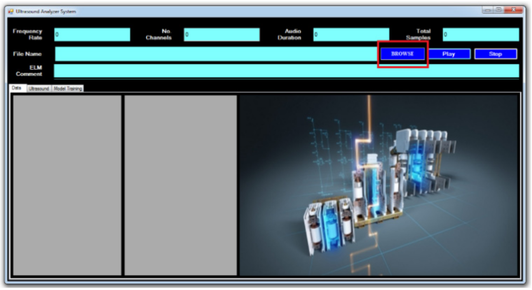
2.3. GUI Classification
2.4. Data Post Processing
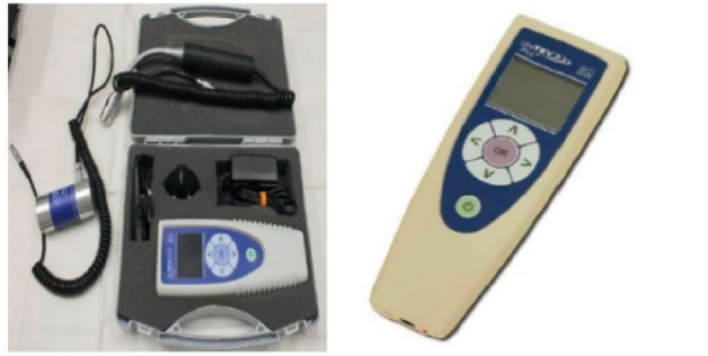
3. Switchgear Data Collection
- Arching—54 sets;
- Corona—41 sets;
- Mechanical—17 sets;
- Tracking—39 sets (available 314 data sets for single-channel wave file);
- Normal—13 sets.
4. Expert Rule
5. Results and Discussion
5.1. Data Pre-Processing
5.2. Raw Data Collection
5.3. Data Analysis and Correlation
5.4. ELM Classification
5.4.1. Corona
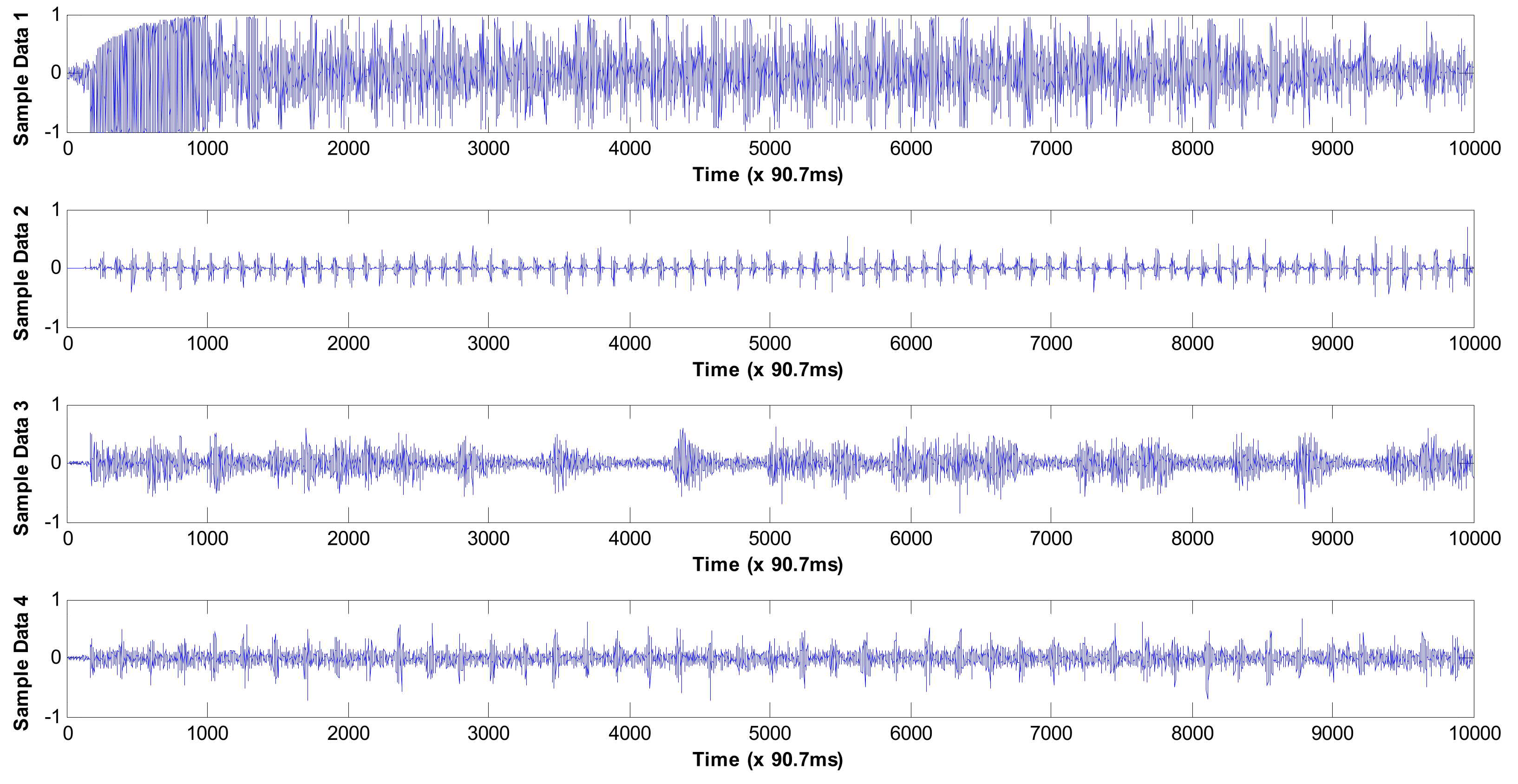
Time Domain
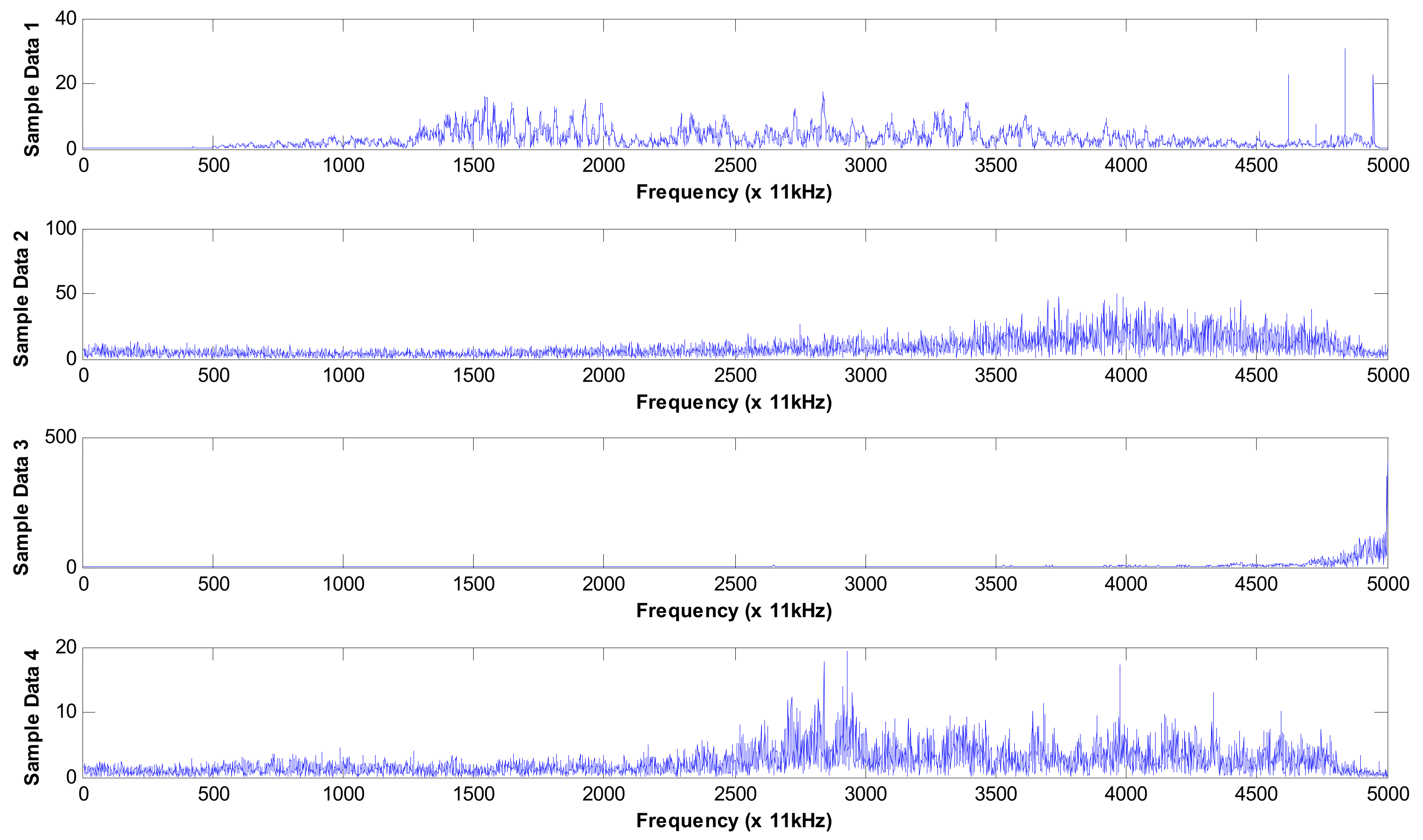
Frequency Domain
5.4.2. Summary
6. Graphical User Interface (GUI) for Ultrasound Analyzer System (UAS)
7. Conclusions
Author Contributions
Funding
Institutional Review Board Statement
Informed Consent Statement
Data Availability Statement
Acknowledgments
Conflicts of Interest
References
- Paoletti, G.; Blokhintsev, I.; Golubev, A. On-Line Condition Assessment of MV Electrical Switchgear and Ancillary Equipment via Partial Discharge Technology. In Proceedings of the EPRI 9th Substation Diagnostics Conference; Available online: https://www.osti.gov/biblio/835368-proceedings-substation-equipment-diagnostics-conference-ix (accessed on 29 September 2021).
- Loo, Y.; Yaw, C.; Hashim, A.; Mohamad, A.; Faizah, M.; Noormala, A. Development of switchgear life cycle cost analysis software. In 2010 4th International Power Engineering and Optimization Conference (PEOCO); IEEE: New York, NY, USA, 2010; pp. 418–423. Available online: https://ieeexplore.ieee.org/abstract/document/5559217 (accessed on 29 September 2021).
- Diessner, A.; Luxa, G.; Neyer, W. Electrical aging tests on epoxy insulators in GIS. IEEE Trans. Electr. Insul. 1989, 24, 277–283. [Google Scholar] [CrossRef]
- Perdon, K.; Scarpellini, M.; Magoni, S.; Cavalli, L. Modular online monitoring system to allow condition-based maintenance for medium voltage switchgear. CIRED-Open Access Proc. J. 2017, 1, 346–349. [Google Scholar] [CrossRef] [Green Version]
- Balobanov, R.; Zaripov, D.; Akhmadeev, A. The device for monitoring the LED display high-voltage insulators state. In IOP Conference Series: Materials Science and Engineering; IOP Publishing: Bristol, UK, 2019; Volume 552, no. 1, p. 012011. Available online: https://iopscience.iop.org/article/10.1088/1757-899X/552/1/012011/meta (accessed on 29 September 2021).
- Kang, W.J.; Park, J.N.; Lee, D.H.; Shin, Y.S.; Kim, Y.K.; Oh, I.S.; Lim, K.J. Development and on-site application of UHF PD detection system to estimate the insulator condition of MV switchgear. In 2008 International Conference on Condition Monitoring and Diagnosis; IEEE: Beijing, China, 2008; pp. 1123–1126. Available online: https://ieeexplore.ieee.org/abstract/document/4580481 (accessed on 29 September 2021).
- Headley, P. Testing requirements for composite insulators for HV switchgear. In IEE Colloquium on Structural Use of Composites in High Voltage Switchgear/Transmission Networks; IET: London, UK, 1992; pp. 4/1–4/5. [Google Scholar]
- Runde, M. Failure frequencies for high-voltage circuit breakers, disconnectors, earthing switches, instrument transformers, and gas-insulated switchgear. IEEE Trans. Power Deliv. 2012, 28, 529–530. [Google Scholar] [CrossRef]
- Velásquez, R.M.A.; Lara, J.V.M.; Melgar, A. Reliability model for switchgear failure analysis applied to ageing. Eng. Fail. Anal. 2019, 101, 36–60. [Google Scholar] [CrossRef]
- Shuxin, L.; Yundong, C.; Chunguang, H.; Xiaoming, L.; Jing, L. Development of on-line monitoring system of switchgear. In 2011 1st International Conference on Electric Power Equipment-Switching Technology; IEEE: Xi’an, China, 2011; pp. 295–298. Available online: https://ieeexplore.ieee.org/abstract/document/6122992 (accessed on 29 September 2021).
- Raju, R.; Narayananaswamy, V.; Durairaj, M.; Vittal, D.P.; Sethuraman, R.; Ananda, R.G.; Aravindakshan, A.M. Design and implementation of compact and robust medium voltage switchgear for deepwater work-class ROV ROSUB 6000. Underw. Technol. 2013, 31, 203–213. [Google Scholar] [CrossRef]
- Chernenko, I.V. Effect of Switchgear Failures in Calculations of Structural Reliability of Power Supply Circuits at Industrial Facilities. In 2018 International Conference on Industrial Engineering, Applications and Manufacturing (ICIEAM); IEEE: Moscow, Russia, 2018; pp. 1–4. Available online: https://ieeexplore.ieee.org/abstract/document/8728587 (accessed on 29 September 2021).
- Purnomoadi, A.; Mor, A.R.; Smit, J. Health index and risk assessment models for Gas Insulated Switchgear (GIS) operating under tropical conditions. Int. J. Electr. Power Energy Syst. 2020, 117, 105681. [Google Scholar] [CrossRef]
- Boettcher, B.; Sinai, A.; Menge, M.; Gräf, T.; Plath, R.; Hücker, T. Algorithms for a Multi-Sensor Partial Discharge Expert System Applied to Medium Voltage Cable Connectors. In 2019 2nd International Conference on High Voltage Engineering and Power Systems (ICHVEPS); IEEE: Denpasar, Indonesia, 2019; pp. 190–195. [Google Scholar]
- Kadechkar, A.; Moreno-Eguilaz, M.; Riba, J.-R.; Capelli, F. Low-cost online contact resistance measurement of power connectors to ease predictive maintenance. IEEE Trans. Instrum. Meas. 2019, 68, 4825–4833. [Google Scholar] [CrossRef]
- Liu, Y.; Jia, Y.-Y.; Yang, J.-G.; Song, S.-Q.; Wu, B.; Li, J. Research of mechanical state diagnosis techniques in GIS bus connector based on mechanical vibration. In 2018 12th International Conference on the Properties and Applications of Dielectric Materials (ICPADM); IEEE: Xi’an, China, 2018; pp. 682–685. [Google Scholar]
- Gauthier, J.; Sonzogni, G. The failure to break test in MV switchboards: An improvement of safety of persons and property. In Proceedings of the 1990 Third International Conference on Future Trends in Distribution Switchgear, London, UK, 23–25 April 1990; pp. 56–60. [Google Scholar]
- Guan, X.; Qin, J.; Shu, N.; Peng, H. Studies on contact degradation process and failure mechanism of GIB plug-in connector. IEEE Trans. Compon. Packag. Manuf. Technol. 2019, 9, 1776–1784. [Google Scholar] [CrossRef]
- Tenbohlen, S.; Denissov, D.; Hoek, S.M.; Markalous, S. Partial discharge measurement in the ultra high frequency (UHF) range. IEEE Trans. Dielectr. Electr. Insul. 2008, 15, 1544–1552. [Google Scholar] [CrossRef]
- Uzelac, M. Test Regimes for HV and EHV Cable Connectors. In Accessories for HV and EHV Extruded Cables: Volume 1: Components; SpringerLinkpp: Berlin/Heidelberg, Germany, 2021; pp. 421–528. [Google Scholar]
- Auckland, D.; McGrail, A.; Smith, C.; Varlow, B.; Zhao, J.; Zhu, D. Application of ultrasound to the inspection of insulation. IEE Proc.-Sci. Meas. Technol. 1996, 143, 177–181. [Google Scholar] [CrossRef]
- Chen, L.-J.; Lin, W.-M.; Tsao, T.-P.; Lin, Y.-H. Study of partial discharge measurement in power equipment using acoustic technique and wavelet transform. IEEE Trans. Power Deliv. 2007, 22, 1575–1580. [Google Scholar] [CrossRef]
- Leighton, T.G. What is ultrasound? Prog. Biophys. Mol. Biol. 2007, 93, 3–83. [Google Scholar] [CrossRef]
- Leighton, T. Are some people suffering as a result of increasing mass exposure of the public to ultrasound in air? Proc. R. Soc. A: Math. Phys. Eng. Sci. 2016, 472, 20150624. [Google Scholar] [CrossRef]
- Maher, R.C. Principles of Forensic Audio Analysis; Springer: Berlin/Heidelberg, Germany, 2018; Available online: https://link.springer.com/book/10.1007%2F978-3-319-99453-6 (accessed on 29 September 2021).
- Soliman, M.H.A. Ultrasound Analysis for Condition Monitoring: Applications of Ultrasound Detection for Various Industrial Equipment. Mohammed Hamed Ahmed Soliman: Berlin/Heidelberg, Germany, 2020. Available online: https://books.google.com.my/books?hl=en&lr=&id=oM4uEAAAQBAJ&oi=fnd&pg=PA3&dq=Ultrasound+Analysis+for+Condition+Monitoring:+Applications+of+Ultrasound+Detection+for+Various+Industrial+Equipment&ots=LHKcKaTnK-&sig=unKxM3VZp0BRImSrJKK_uv7RJck&redir_esc=y#v=onepage&q=Ultrasound%20Analysis%20for%20Condition%20Monitoring%3A%20Applications%20of%20Ultrasound%20Detection%20for%20Various%20Industrial%20Equipment&f=false (accessed on 29 September 2021).
- Brady, J.; Thermographer, L.-I.C. Corona and Tracking Conditions in Metal-Clad Switchgear Case Studies; Brady Infrared Insp: Stuart, FL, USA, 2006. [Google Scholar]
- Javed, H.; Kang, L.; Zhang, G. The Study of Different Metals Effect on Ozone Generation Under Corona Discharge in MV Switchgear Used for Fault Diagnostic. In Proceedings of the 2019 IEEE Asia Power and Energy Engineering Conference (APEEC), Chengdu, China, 29–31 March 2019; pp. 29–33. [Google Scholar]
- Weichert, H.; Benz, P.; Hill, N.; Hilbert, M.; Kurrat, M. On Partial Discharge/Corona Considerations for Low Voltage Switchgear and Controlgear. In 2018 IEEE Holm Conference on Electrical Contacts; IEEE: Albuquerque, NM, USA, 2018; pp. 246–253. [Google Scholar]
- Ishak, S.; Koh, S.-P.; Tan, J.-D.; Tiong, S.-K.; Chen, C.-P. Corona fault detection in switchgear with extreme learning machine. Bull. Electr. Eng. Inform. 2020, 9, 558–564. [Google Scholar] [CrossRef]
- Tang, J.; Liu, F.; Zhang, X.; Ren, X.; Fan, M. Characteristics of the Concentration Ratio of SO2F2 to SOF2 as the Decomposition Products of SF6 Under Corona Discharge. IEEE Trans. Plasma Sci. 2011, 40, 56–62. [Google Scholar] [CrossRef]
- Raj, A.; Ishak, S.; Amir, M.; Yogendra, B.; Raffi, M. Corona Detection Using Wide Band Antenna and Time Delay Method. Telkomnika 2017, 15, 1547–1553. [Google Scholar] [CrossRef] [Green Version]
- Cho, H.-S. Frequency Spectrum Analysis of Corona Discharge Source Measured by Ultrasound Detector. J. Korea Inst. Inf. Electron. Commun. Technol. 2019, 12, 78–82. [Google Scholar]
- Chidurala, M. Electrical Equipment Reliability with Ultrasound. Water Energy Int. 2016, 59, 16–18. [Google Scholar]
- Haiguo, T.; Jiran, Z.; Fangliang, G.; Hua, L.; Min, F.; Qi, H. Research on a rail-robot based remote three-dimensional inspection system for switch stations in power distribution network. In Proceedings of the 2017 Chinese Automation Congress (CAC), Jinan, Xian, 20–22 October 2017; pp. 7925–7930. [Google Scholar]
- Baug, A.; Choudhury, N.R.; Ghosh, R.; Dalai, S.; Chatterjee, B. Identification of single and multiple partial discharge sources by optical method using mathematical morphology aided sparse representation classifier. IEEE Trans. Dielectr. Electr. Insul. 2017, 24, 3703–3712. [Google Scholar] [CrossRef]
- Hussain, G.A.; Kumpulainen, L.; Klüss, J.V.; Lehtonen, M.; Kay, J.A. The smart solution for the prediction of slowly developing electrical faults in MV switchgear using partial discharge measurements. IEEE Trans. Power Deliv. 2013, 28, 2309–2316. [Google Scholar] [CrossRef]
- Paoletti, G.; Baier, M. Failure contributors of MV electrical equipment and condition assessment program development. In Proceedings of the Conference Record of 2001 Annual Pulp and Paper Industry Technical Conference (Cat. No. 01CH37209), Portland, OR, USA, 18–22 June 2001; pp. 37–47. [Google Scholar]
- Tahan, M.; Muhammad, M.; Karim, Z.A. A framework for intelligent condition-based maintenance of rotating equipment using mechanical condition monitoring. In Proceedings of the MATEC Web of Conferences, Pilsen, Czech Republic, 7–9 September 2021; p. 05011. [Google Scholar]
- Hwang, H.; Lee, J.; Hwang, J.; Jun, H. A study of the development of a condition-based maintenance system for an LNG FPSO. Ocean Eng. 2018, 164, 604–615. [Google Scholar] [CrossRef]
- Vogl, G.W.; Weiss, B.A.; Helu, M. A review of diagnostic and prognostic capabilities and best practices for manufacturing. J. Intell. Manuf. 2019, 30, 79–95. [Google Scholar] [CrossRef]
- Goyal, D.; Pabla, B.; Dhami, S.; Lachhwani, K. Optimization of condition-based maintenance using soft computing. Neural Comput. Appl. 2017, 28, 829–844. [Google Scholar] [CrossRef]
- Tahan, M.; Tsoutsanis, E.; Muhammad, M.; Karim, Z.A. Performance-based health monitoring, diagnostics and prognostics for condition-based maintenance of gas turbines: A review. Appl. Energy 2017, 198, 122–144. [Google Scholar] [CrossRef] [Green Version]
- Hoffmann, M.W.; Wildermuth, S.; Gitzel, R.; Boyaci, A.; Gebhardt, J.; Kaul, H.; Amihai, I.; Forg, B.; Suriyah, M.; Leibfried, T. Integration of novel sensors and machine learning for predictive maintenance in medium voltage switchgear to enable the energy and mobility revolutions. Sensors 2020, 20, 2099. [Google Scholar] [CrossRef] [PubMed] [Green Version]
- Zheng, K.; Si, G.; Diao, L.; Zhou, Z.; Chen, J.; Yue, W. Applications of support vector machine and improved k-Nearest Neighbor algorithm in fault diagnosis and fault degree evaluation of gas insulated switchgear. In Proceedings of the 2017 1st International Conference on Electrical Materials and Power Equipment (ICEMPE), Xian, China, 14–17 May 2017; pp. 364–368. [Google Scholar]
- Nguyen, M.-T.; Nguyen, V.-H.; Yun, S.-J.; Kim, Y.-H. Recurrent neural network for partial discharge diagnosis in gas-insulated switchgear. Energies 2018, 11, 1202. [Google Scholar] [CrossRef] [Green Version]
- Wang, Y.; Yan, J.; Yang, Z.; Liu, T.; Zhao, Y.; Li, J. Partial discharge pattern recognition of gas-insulated switchgear via a light-scale convolutional neural network. Energies 2019, 12, 4674. [Google Scholar] [CrossRef] [Green Version]
- Yuan, Y.; Ma, S.; Wu, J.; Jia, B.; Li, W.; Luo, X. Fault diagnosis in gas insulated switchgear based on genetic algorithm and density-based spatial clustering of applications with noise. IEEE Sens. J. 2019, 21, 965–973. [Google Scholar] [CrossRef]
- Gong, Y.; Liu, Y.; Wu, L. Identification of partial discharge in gas insulated switchgears with fractal theory and support vector machine. Power Syst. Technol. 2011, 35, 135–139. [Google Scholar]
- Wang, Y.; Yan, J.; Jing, Q.; Qi, Z.; Wang, J.; Geng, Y. A novel adversarial transfer learning in deep convolutional neural network for intelligent diagnosis of gas-insulated switchgear insulation defect: A DATCNN for GIS insulation defect diagnosis. IET Gener. Trans. Distrib. 2021. [Google Scholar] [CrossRef]
- Sukma, T.R.; Khayam, U.; Sugawara, R.; Yoshikawa, H.; Kozako, M.; Hikita, M.; Eda, O.; Otsuka, M.; Kaneko, H.; Shiina, Y. Determination of type of partial discharge in cubicle-type gas insulated switchgear (C-GIS) using artificial neural network. In Proceedings of the 2018 Condition Monitoring and Diagnosis (CMD), Perth, Western Australia, 23–26 September 2018; pp. 1–5. [Google Scholar]
- Zhiwei, L.; Kehui, Z.; Xiaochun, Z. Research on Fault Diagnosis of Switchgear Contacts Based on BP Neural Network. In Proceedings of the 2018 International Conference on Power System Technology (POWERCON), Guangzhou, China, 6–9 November 2018; pp. 3507–3513. [Google Scholar]
- Barrios, S.; Buldain, D.; Comech, M.P.; Gilbert, I. Partial Discharge Identification in MV switchgear using Scalogram representations and Convolutional AutoEncoder. IEEE Trans. Power Deliv. 2020. Available online: https://ieeexplore.ieee.org/abstract/document/9286573 (accessed on 29 September 2021). [CrossRef]
- Tuyet-Doan, V.-N.; Pho, H.-A.; Lee, B.; Kim, Y.-H. Deep Ensemble Model for Unknown Partial Discharge Diagnosis in Gas-Insulated Switchgears Using Convolutional Neural Networks. IEEE Access 2021, 9, 80524–80534. [Google Scholar] [CrossRef]
- Zhang, J.-M.; Yin, J.-H.; Jiang, X.-X. Application of RBF network-based state assessment technique of high voltage switchgear to intelligent GIS. High Volt. Appar. 2013, 49, 115–121. [Google Scholar]
- Xue, W. Improved method of high voltage switchgear temperature prediction based on WNN. Appl. Mech. Mater. 2014, 644–650, 502–505. Available online: https://www.scientific.net/AMM.644-650.502 (accessed on 29 September 2021). [CrossRef]
- Feng, X.; Zhou, Y.; Hua, T.; Zou, Y.; Xiao, J. Contact temperature prediction of high voltage switchgear based on multiple linear regression model. In Proceedings of the 2017 32nd Youth Academic Annual Conference of Chinese Association of Automation (YAC), Hefei, China, 19–21 May 2018; pp. 277–280. [Google Scholar]
- Qiao, X.; Gao, K.; Huang, H.; Lyu, L.; Lin, W.; Jin, L. Temperature Rise Prediction of GIS Electrical Contact Using an Improved Kalman Filter. In Proceedings of the IECON 2019–45th Annual Conference of the IEEE Industrial Electronics Society, Lisbon, Portugal, 14–17 September 2019; pp. 167–172. [Google Scholar]
- Huang, G.-B.; Wang, D.H.; Lan, Y. Extreme learning machines: A survey. Int. J. Mach. Learn. Cybern. 2011, 2, 107–122. [Google Scholar] [CrossRef]
- Huang, G.; Huang, G.-B.; Song, S.; You, K. Trends in extreme learning machines: A review. Neural Netw. 2015, 61, 32–48. [Google Scholar] [CrossRef] [PubMed]
- Huang, G.; Song, S.; Gupta, J.N.; Wu, C. Semi-supervised and unsupervised extreme learning machines. IEEE Trans. Cybern. 2014, 44, 2405–2417. [Google Scholar] [CrossRef]
- Deng, C.; Huang, G.; Xu, J.; Tang, J. Extreme learning machines: New trends and applications. Sci. China Inf. Sci. 2015, 58, 1–16. [Google Scholar] [CrossRef] [Green Version]
- Huang, G.-B. An insight into extreme learning machines: Random neurons, random features and kernels. Cogn. Comput. 2014, 6, 376–390. [Google Scholar] [CrossRef]
- Yaw, C.T.; Yap, K.S.; Wong, S.Y.; Yap, H.J.; Paw, J.K.S. Enhancement of Neural Network Based Multi Agent System for Classification and Regression in Energy System. IEEE Access 2020, 8, 163026–163043. [Google Scholar] [CrossRef]
- Yadav, B.; Ch, S.; Mathur, S.; Adamowski, J. Assessing the suitability of extreme learning machines (ELM) for groundwater level prediction. J. Water Land Dev. 2017, 103–112. [Google Scholar] [CrossRef]
- Bartlett, P.L. The sample complexity of pattern classification with neural networks: The size of the weights is more important than the size of the network. IEEE Trans. Inf. Theory 1998, 44, 525–536. [Google Scholar] [CrossRef] [Green Version]
- Huang, G.-B.; Zhu, Q.-Y.; Siew, C.-K. Extreme learning machine: A new learning scheme of feedforward neural networks. In Proceedings of the 2004 IEEE International Joint Conference on Neural Networks (IEEE Cat. No. 04CH37541), Budapest, Hungary, 25–29 July 2004; pp. 985–990. [Google Scholar]
- Pacheco, A.G.; Krohling, R.A.; da Silva, C.A. Restricted Boltzmann machine to determine the input weights for extreme learning machines. Expert Syst. Appl. 2018, 96, 77–85. [Google Scholar] [CrossRef] [Green Version]
- Yaw, C.T.; Wong, S.Y.; Yap, K.S.; Yap, H.J.; Amirulddin, U.A.U.; Tan, S.C. An ELM based multi-agent system and its applications to power generation. Intell. Decis. Technol. 2018, 12, 163–171. [Google Scholar] [CrossRef]
- Luo, M.; Zhang, K. A hybrid approach combining extreme learning machine and sparse representation for image classification. Eng. Appl. Artif. Intell. 2014, 27, 228–235. [Google Scholar] [CrossRef]
- Lu, S.; Wang, X.; Zhang, G.; Zhou, X. Effective algorithms of the Moore-Penrose inverse matrices for extreme learning machine. Intell. Data Anal. 2015, 19, 743–760. [Google Scholar] [CrossRef] [Green Version]
- Tang, J.; Deng, C.; Huang, G.-B. Extreme learning machine for multilayer perceptron. IEEE Trans. Neural Netw. Learn. Syst. 2015, 27, 809–821. [Google Scholar] [CrossRef]
- Huang, G.-B.; Zhu, Q.-Y.; Siew, C.-K. Extreme learning machine: Theory and applications. Neurocomputing 2006, 70, 489–501. [Google Scholar] [CrossRef]
- Muhamad, N.A.; Musa, I.V.; Malek, Z.A.; Mahdi, A.S. Classification of Partial Discharge Fault Sources on SF₆ Insulated Switchgear Based on Twelve By-Product Gases Random Forest Pattern Recognition. IEEE Access 2020, 8, 212659–212674. [Google Scholar] [CrossRef]


| Audio File | Basic Information | Sampling Rates |
|---|---|---|
| Arc.wav | NumChannels: 1 SampleRate: 11,025 bit/s TotalSamples: 68,900 bits Duration: 6.2494 s BitsPerSample: 16 bps |
|
| Corona.wav | NumChannels: 1 SampleRate: 8000 bit/s TotalSamples: 53,991 bits Duration: 6.7489 s BitsPerSample: 8 bps | |
| Tracking.wav | NumChannels: 1 SampleRate: 8000 bit/s TotalSamples: 52,000 bits Duration: 6.5000 s BitsPerSample: 8 bps | |
| Good Bearing.wav | NumChannels: 1 SampleRate: 11,025 bit/s TotalSamples: 48,551 bits Duration: 4.4037 s BitsPerSample: 16 bps | |
| Bad Bearing.wav | NumChannels: 1 SampleRate: 11,025 bit/s TotalSamples: 55,301 bits Duration: 5.0160 s BitsPerSample: 16 bps |
| Fault Type | Ultrasound Amplitude | |
|---|---|---|
| Min | Max | |
| Normal | ≥−0.015 | ≤0.015 |
| Corona | ≥−0.2 | ≤0.2 |
| Arching | ≥−0.8 | ≤0.8 |
| Tracking | <−0.8 | >0.8 |
| No. | Equipment | Sampling Rate (Bits/Second) | File Format |
|---|---|---|---|
| 1. | UltraTEV Plus | 11,025 | mp3 |
| 16,000 | |||
| 22,000 | |||
| 2. | UltraTEV Plus 2 | 11,025 | wav |
| 16,000 | |||
| 22,000 | |||
| 44,100 | |||
| 3. | Ultraprobe 9000 | 8000 | wav |
| 11,025 | |||
| 16,000 | |||
| 22,000 | |||
| 4. | Ultraprobe 10,000 | 8000 | wav |
| 11,025 | |||
| 16,000 | |||
| 22,000 | |||
| 44,100 |
| No. | Types of Faults | Cases |
|---|---|---|
| 1. | Normal | 314 |
| 2. | Corona | 160 |
| 3. | Tracking | 149 |
| 4. | Arcing | 203 |
| 5. | Mechanical | 15 |
| No. | Date | Substation | Affected Area | Finding/Remarks |
|---|---|---|---|---|
| 1. | 17 March 2018 | PMU Iaduks 33 kV, Johor Bahru | Breaker compartment | Corona
|
| 2. | 22 March 2018 | PE Sekolah Kebangsaan Aur Atok 11 kV, Kedah | Feeder Kg Lintang, Back panel | Surface Discharge
|
| 3. | 11 March 2018 | PMU Aysamet 33 kV, Selangor | Cable Compartment, Yellow phase bushing | Arcing
|
| Time Domain | |||
|---|---|---|---|
| Training | Validation | Testing | |
| No Sample | 128 | 24 | 8 |
| Accuracy Rate | 90.63% | 87.5% | 87.5% |
| Error Rate | 9.37% | 12.5% | 12.5% |
| Feature Number | 10,000 | ||
| Hidden Neuron | 1200 | ||
| Output Number | 1 | ||
| Training Phase | |||
|---|---|---|---|
| Classified Class | |||
| Corona | Non-Corona | ||
| Actual Class | Corona | 26 | 3 |
| Non-Corona | 9 | 90 | |
| Accuracy Rate | 90.63% | ||
| Error Rate | 9.37% | ||
| Validation Phase | |||
|---|---|---|---|
| Classified Class | |||
| Corona | Non-Corona | ||
| Actual Class | Corona | 1 | 1 |
| Non-Corona | 2 | 20 | |
| Accuracy Rate | 87.5% | ||
| Error Rate | 12.5% | ||
| Testing Phase | |||
|---|---|---|---|
| Classified Class | |||
| Corona | Non-Corona | ||
| Actual Class | Corona | 1 | 1 |
| non-Corona | 0 | 6 | |
| Accuracy Rate | 87.5% | ||
| Error Rate | 12.5% | ||
| Frequency Domain | |||
|---|---|---|---|
| Training | Validation | Testing | |
| No Sample | 128 | 24 | 8 |
| Accuracy Rate | 89.84% | 83.33% | 87.5% |
| Error Rate | 10.16% | 16.67% | 12.5% |
| Feature Number | 5000 | ||
| Hidden Neuron | 150 | ||
| Output Number | 1 | ||
| Training Phase | |||
|---|---|---|---|
| Classified Class | |||
| Corona | Non-Corona | ||
| Actual Class | Corona | 21 | 3 |
| Non-Corona | 10 | 94 | |
| Accuracy Rate | 89.84% | ||
| Error Rate | 10.16% | ||
| Validation Phase | |||
|---|---|---|---|
| Classified Class | |||
| Corona | Non-Corona | ||
| Actual Class | Corona | 3 | 2 |
| Non-Corona | 2 | 17 | |
| Accuracy Rate | 83.33% | ||
| Error Rate | 16.67% | ||
| Testing Phase | |||
|---|---|---|---|
| Classified Class | |||
| Corona | Non-Corona | ||
| Actual Class | Corona | 2 | 0 |
| Non-Corona | 1 | 5 | |
| Accuracy Rate | 87.5% | ||
| Error Rate | 12.5% | ||
| Accuracy Rate (%) | ||||
|---|---|---|---|---|
| Training | Validation | Testing | ||
| ARCING | Time Domain | 93.75 | 95.83 | 87.5 |
| Frequency Domain | 93.75 | 91.67 | 100 | |
| CORONA | Time Domain | 90.63 | 87.5 | 87.5 |
| Frequency Domain | 89.84 | 83.33 | 87.5 | |
| MECHANICAL | Time Domain | 96.09 | 91.67 | 100 |
| Frequency Domain | 96.09 | 95.83 | 100 | |
| TRACKING | Time Domain | 96.88 | 95.33 | 100 |
| Frequency Domain | 96.88 | 91.67 | 100 | |
| NORMAL | Time Domain | 100 | 95.83 | 100 |
| Frequency Domain | 100 | 95.83 | 100 | |
| Min | 89.84 | 83.33 | 87.5 | |
| max | 100 | 95.83 | 100 | |
| Average | 95.391 | 92.449 | 96.25 | |
| Error Rate (%) | ||||
|---|---|---|---|---|
| Training | Validation | Testing | ||
| ARCING | Time Domain | 6.25 | 4.17 | 12.5 |
| Frequency Domain | 6.25 | 8.33 | 0 | |
| CORONA | Time Domain | 9.37 | 12.5 | 12.5 |
| Frequency Domain | 10.16 | 16.67 | 12.5 | |
| MECHANICAL | Time Domain | 3.91 | 8.33 | 0 |
| Frequency Domain | 3.91 | 4.17 | 0 | |
| TRACKING | Time Domain | 3.12 | 4.67 | 0 |
| Frequency Domain | 3.12 | 8.33 | 0 | |
| NORMAL | Time Domain | 0 | 4.17 | 0 |
| Frequency Domain | 0 | 4.17 | 0 | |
| Min | 0 | 4.17 | 0 | |
| max | 10.16 | 16.67 | 12.5 | |
| Average | 4.609 | 7.551 | 3.75 | |
| Approaches | Classification Accuracy Rate (%) |
|---|---|
| ELMARCING | 95.83 |
| ELMCORONA | 87.5 |
| ELMMECHANICAL | 91.67 |
| ELMTRACKING | 95.33 |
| ELMNORMAL | 95.83 |
| Random Forest [74] | 87.5 |
| Decision Tree [74] | 22.9 |
| Decision Stump [74] | 50 |
| Decision Table [74] | 58.3 |
| Multilayer Perceptron [74] | 51 |
| Optimized Feature Space—Support Vector Machine (GFS-SVM) [48] | 90 |
| Original Feature Space—Support Vector Machine (OFS-SVM) [48] | 69.2 |
| Optimized Feature Space—Random Forest (GFS-RF) [48] | 86.3 |
| Original Feature Space—Random Forest (OFS-RF) [48] | 77.92 |
| Optimized Feature Space—Density-Based Spatial Clustering of Applications with Noise (GFS-DBSCAN) [48] | 98.3 |
| Classified Results | Time-Domain | Frequency-Domain | ||||||
|---|---|---|---|---|---|---|---|---|
| Corona | Arcing | Tracking | Mechanical | Corona | Arcing | Tracking | Mechanical | |
| Arcing and Mechanical | 1 | 0 | 0 | 1 | 0 | 1 | 0 | 0 |
| Tracking | 1 | 1 | 1 | 0 | 0 | 1 | 0 | 0 |
| Corona and Mechanical | 1 | 0 | 0 | 1 | 1 | 0 | 0 | 1 |
| Tracking | 0 | 1 | 0 | 0 | 0 | 0 | 1 | 0 |
| Tracking and Mechanical | 1 | 0 | 1 | 1 | 1 | 1 | 0 | 0 |
| Arcing | 1 | 1 | 0 | 0 | 0 | 1 | 0 | 0 |
| ELM Output | Expert Rule Output | Final Output | |
|---|---|---|---|
| Scenario 1 | Normal | Any | Normal |
| Scenario 2 | Corona | Any | Corona |
| Scenario 3 | Tracking | Tracking | Tracking |
| Scenario 4 | Tracking | Arcing | Arcing |
| Scenario 5 | Arcing | Tracking | Tracking |
| Scenario 6 | Mechanical | Any | Mechanical |
Publisher’s Note: MDPI stays neutral with regard to jurisdictional claims in published maps and institutional affiliations. |
© 2021 by the authors. Licensee MDPI, Basel, Switzerland. This article is an open access article distributed under the terms and conditions of the Creative Commons Attribution (CC BY) license (https://creativecommons.org/licenses/by/4.0/).
Share and Cite
Ishak, S.; Yaw, C.T.; Koh, S.P.; Tiong, S.K.; Chen, C.P.; Yusaf, T. Fault Classification System for Switchgear CBM from an Ultrasound Analysis Technique Using Extreme Learning Machine. Energies 2021, 14, 6279. https://doi.org/10.3390/en14196279
Ishak S, Yaw CT, Koh SP, Tiong SK, Chen CP, Yusaf T. Fault Classification System for Switchgear CBM from an Ultrasound Analysis Technique Using Extreme Learning Machine. Energies. 2021; 14(19):6279. https://doi.org/10.3390/en14196279
Chicago/Turabian StyleIshak, Sanuri, Chong Tak Yaw, Siaw Paw Koh, Sieh Kiong Tiong, Chai Phing Chen, and Talal Yusaf. 2021. "Fault Classification System for Switchgear CBM from an Ultrasound Analysis Technique Using Extreme Learning Machine" Energies 14, no. 19: 6279. https://doi.org/10.3390/en14196279
APA StyleIshak, S., Yaw, C. T., Koh, S. P., Tiong, S. K., Chen, C. P., & Yusaf, T. (2021). Fault Classification System for Switchgear CBM from an Ultrasound Analysis Technique Using Extreme Learning Machine. Energies, 14(19), 6279. https://doi.org/10.3390/en14196279