
Numerical Modeling of the Interference of Thermally Unbalanced Aquifer Thermal Energy Storage Systems in Brussels (Belgium)


Abstract
:1. Introduction
2. Materials and Methods
2.1. Context
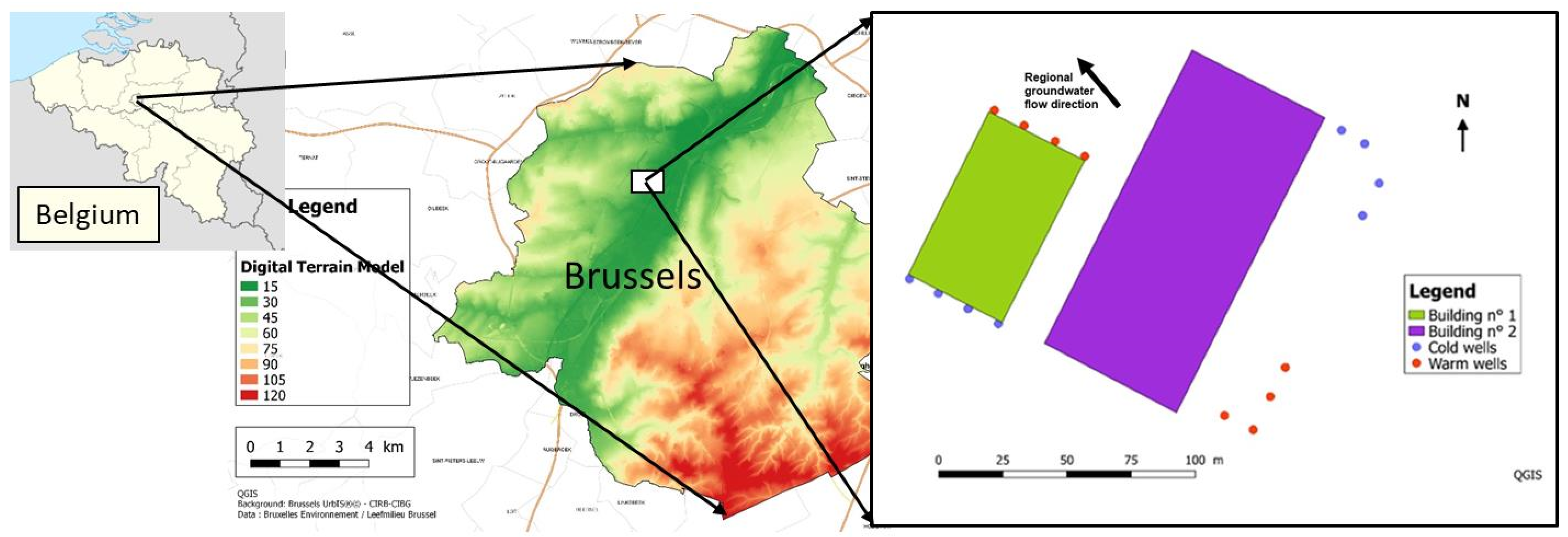
2.2. Study Case
2.2.1. Problem Statement
2.2.2. Hydrogeology Context
2.3. Methods
2.3.1. Groundwater Flow and Heat Transport Equations
2.3.2. Conceptual Model
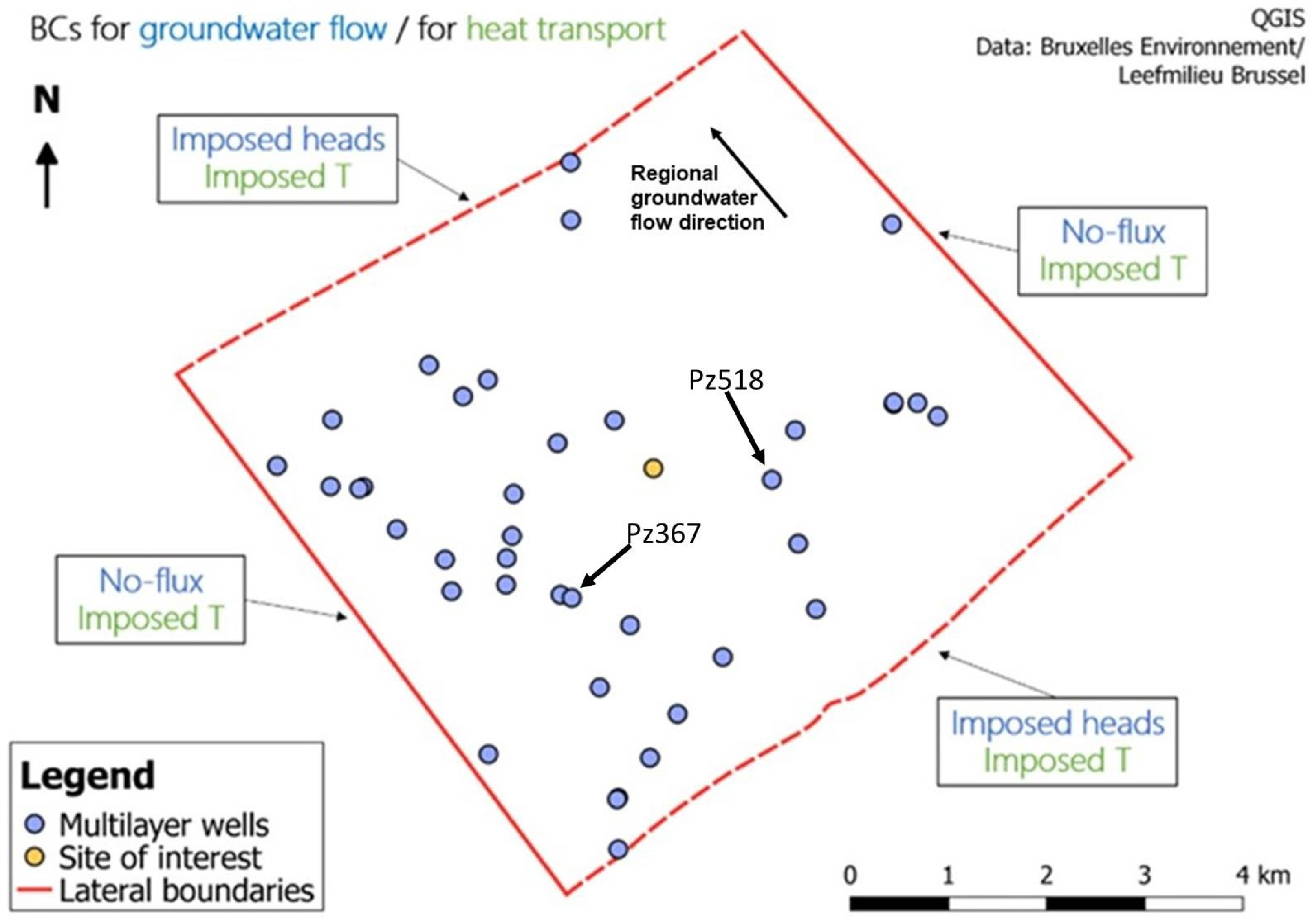
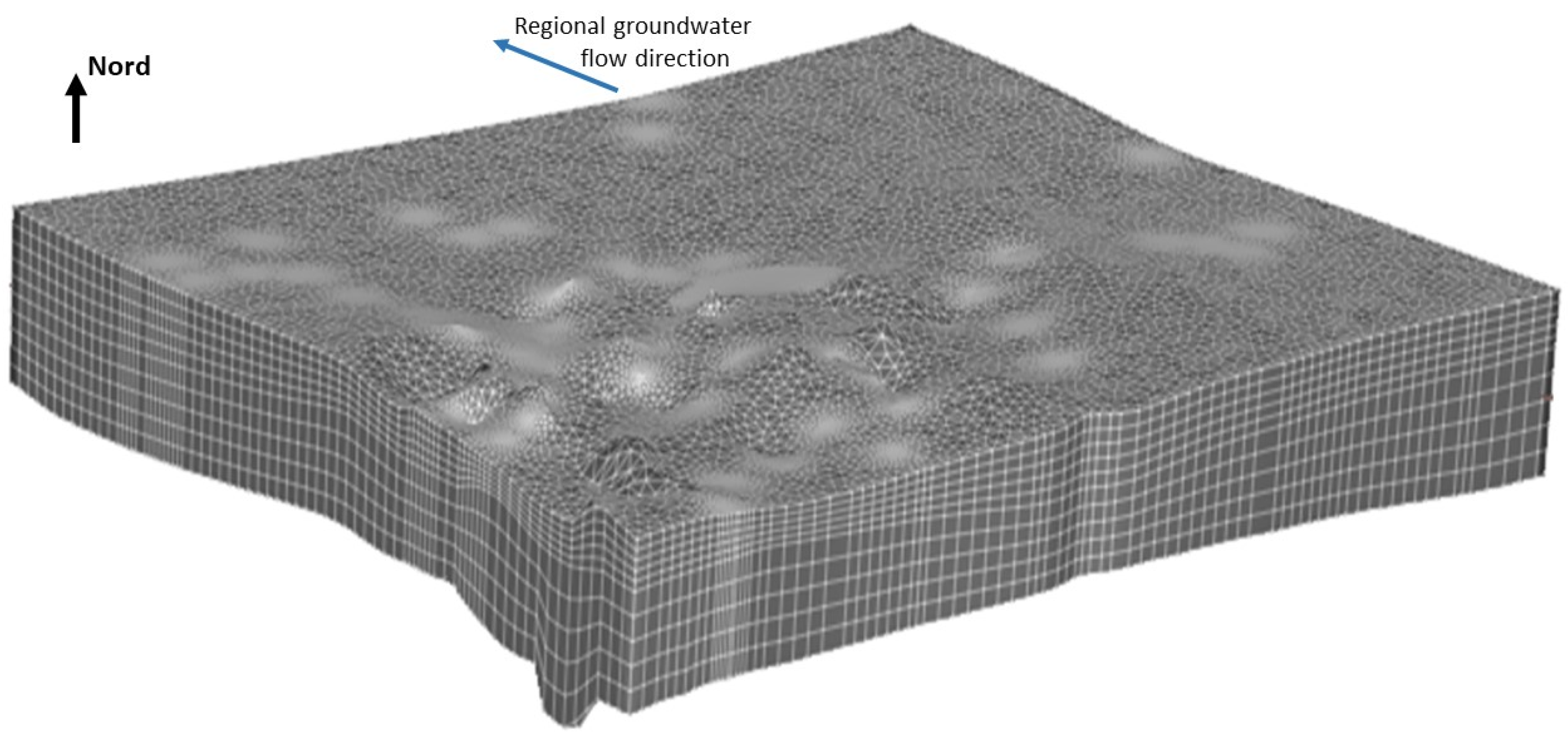
2.3.3. Numerical Model
- on the upper and lower boundaries: zero-flux BCs;
- along the SE and NW boundaries: imposed piezometric heads, representative of the piezometric level observed during the simulated period;
- along the NE and SW boundaries: zero-flux BCs;
- in abstraction wells: imposed flux, equal to the average annual abstracted flow rate.
- The defined heat transport BCs are (Figure 2):
- on the upper and lower boundaries: zero-diffusive flux BCs;
- along lateral boundaries: imposed temperature, equal to the undisturbed background temperature.
3. Results
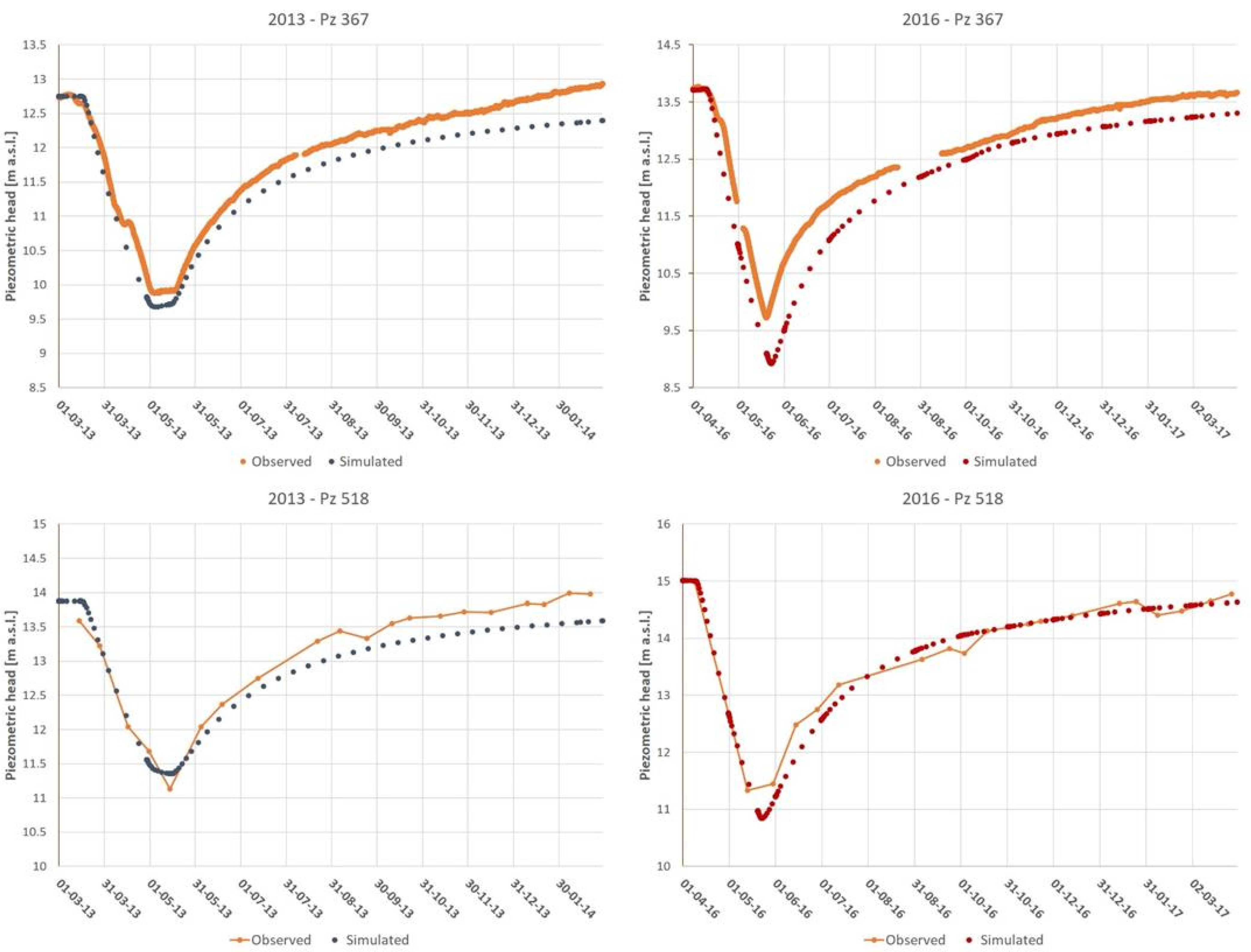
3.1. Groundwater Flow Calibration
3.2. Heat Transport Simulations
3.2.1. Scenario Descriptions
3.2.2. Simulation Results
4. Discussion
- increased use of heat during winter by providing heat to neighboring buildings;
- ncreased night ventilation and window solar protection during the summer.
Author Contributions
Funding
Informed Consent Statement
Data Availability Statement
Acknowledgments
Conflicts of Interest
References
- Dassargues, A. Hydrogeology-Groundwater Science and Engineering; Taylor & Francis CRC Press: Boca Raton, FL, USA, 2018; pp. 323–343. [Google Scholar]
- Dassargues, A. Hydrogéologie Appliquée-Science et Ingéniérie des Eaux Souterraines; Dunod: Paris, France, 2020; pp. 341–364. (In French) [Google Scholar]
- Fleuchaus, P.; Godschalk, B.; Stober, I.; Blum, P. Worldwide application of aquifer thermal energy storage—A review. Renew. Sustain. Energy Rev. 2018, 94, 861–876. [Google Scholar] [CrossRef]
- Sommer, W.; Valstar, J.; Leusbrock, I.; Grotenhuis, T.; Rijnaarts, H. Optimization and spatial pattern of large-scale aquifer thermal energy storage. Appl. Energy 2015, 137, 322–337. [Google Scholar] [CrossRef]
- Vanhoudt, D.; Desmedt, J.; Van Bael, J.; Robeyn, N.; Hoes, H. An aquifer thermal storage system in a Belgian hospital: Long-term experimental evaluation of energy and cost savings. Energy Build. 2011, 43, 3657–3665. [Google Scholar] [CrossRef]
- Gao, L.; Zhao, J.; An, Q.; Wang, J.; Liu, X. A review on system performance studies of aquifer thermal energy storage. Energy Procedia 2017, 142, 3537–3545. [Google Scholar] [CrossRef]
- Possemiers, M.; Huysmans, M.; Batelaan, O. Influence of aquifer thermal energy storage on groundwater quality: A review illustrated by seven case studies from Belgium. J. Hydrol. Reg. Stud. 2014, 2, 20–34. [Google Scholar] [CrossRef]
- BRUGEO. Cadastre des Systèmes Géothermiques; 2016. Available online: http://geothermie.brussels/fr/geothermie-a-bruxelles/cadastre-des-systemes-geothermiques (accessed on 21 May 2020). (In French).
- De Schepper, G.; Bolly, P.-Y.; Vizzotto, P.; Wecxsteen, H.; Robert, T. Investigations into the first operational aquifer thermal energy storage system in Wallonia (Belgium): What can potentially be expected? Geosciences 2020, 10, 33. [Google Scholar] [CrossRef] [Green Version]
- Anibas, C.; Kukral, J.; Possemiers, M.; Huysmans, M. Assessment of seasonal aquifer thermal energy storage as a groundwater ecosystem service for the Brussels-Capital Region: Combining groundwater flow, and heat and reactive transport modelling. Energy Procedia 2016, 97, 179–185. [Google Scholar] [CrossRef] [Green Version]
- Haehnlein, S.; Bayer, P.; Blum, P. International legal status of the use of shallow geothermal energy. Renew. Sustain. Energy Rev. 2010, 14, 2611–2625. [Google Scholar] [CrossRef]
- Tsagarakis, K.P.; Efthymiou, L.; Michopoulos, A.; Mavragani, A.; Anđelković, A.S.; Antolini, F.; Bacic, M.; Bajare, D.; Baralis, M.; Bogusz, W.; et al. A review of the legal framework in shallow geothermal energy in selected European countries: Need for guidelines. Renew. Energy 2020, 147, 2556–2571. [Google Scholar] [CrossRef]
- Bloemendal, M.; Olsthoorn, T.; Boons, F. How to achieve optimal and sustainable use of the subsurface for Aquifer Thermal Energy Storage. Energy Policy 2014, 66, 104–114. [Google Scholar] [CrossRef]
- Garcia-Gil, A.; Goetlz, G.; Klonowski, M.; Borovic, S.; Boon, D.; Abesser, C.; Janza, M.; Herms, I.; Petitclerc, E.; Erlström, M.; et al. Governance of shallow geothermal energy resources. Energy Policy 2020, 138, 111283. [Google Scholar] [CrossRef]
- Hamada, Y.; Marutani, K.; Nakamura, M.; Nagasaka, S.; Ochifuji, K.; Fuchigami, S.; Yokoyama, S. Study on underground thermal characteristics by using digital national land information, and its application for energy utilization. Appl. Energy 2002, 72, 659–675. [Google Scholar] [CrossRef]
- Lo Russo, S.; Civita, M.V. Open-loop groundwater heat pumps development for large buildings: A case study. Geothermics 2009, 38, 335–345. [Google Scholar] [CrossRef]
- Andrews, C. The impact of the use of heat pumps on ground-water temperatures. Ground Water 1978, 16, 437–443. [Google Scholar] [CrossRef]
- Molina-Giraldo, N.; Bayer, P.; Blum, P. Evaluating the influence of thermal dispersion on temperature plumes from geothermal systems using analytical solutions. Int. J. Therm. Sci. 2011, 50, 1223–1231. [Google Scholar] [CrossRef]
- Graf, T.; Therrien, R. Variable-density groundwater flow and solute transport in porous media containing non-uniform discrete fractures. Adv. Water Resour. 2005, 28, 1351–1367. [Google Scholar] [CrossRef]
- Ma, R.; Zheng, C. Effects of density and viscosity in modeling heat as a groundwater tracer. Ground Water 2010, 48, 380–389. [Google Scholar] [CrossRef] [PubMed]
- Vandenbohede, A.; Hermans, T.; Nguyen, F.; Lebbe, L. Shallow heat injection and storage experiment: Heat transport simulation and sensitivity analysis. J. Hydrol. 2011, 409, 262–272. [Google Scholar] [CrossRef]
- Wildemeersch, S.; Jamin, P.; Orban, P.; Hermans, T.; Klepikova, M.; Nguyen, F.; Brouyère, S.; Dassargues, A. Coupling heat and chemical tracer experiments for estimating heat transfer parameters in shallow alluvial aquifers. J. Contam. Hydrol. 2014, 169, 90–99. [Google Scholar] [CrossRef] [PubMed]
- Wagner, V.; Li, T.; Bayer, P.; Leven, C.; Dietrich, P.; Blum, P. Thermal tracer testing in a sedimentary aquifer: Field experiment (Lauswiesen, Germany) and numerical simulation. Hydrogeol. J. 2014, 22, 175–187. [Google Scholar] [CrossRef]
- Hermans, T.; Wildemeersch, S.; Jamin, P.; Orban, P.; Brouyère, S.; Dassargues, A.; Nguyen, F. Quantitative temperature monitoring of a heat tracing experiment using cross-borehole ERT. Geothermics 2015, 53, 14–26. [Google Scholar] [CrossRef] [Green Version]
- Casasso, A.; Sethi, R. Modelling thermal recycling occurring in groundwater heat pumps (GWHPs). Renew. Energy 2015, 77, 86–93. [Google Scholar] [CrossRef] [Green Version]
- Lo Russo, S.; Taddia, G.; Cerino Abdin, E.; Verda, V. Effects of different re-injection systems on the thermal affected zone (TAZ) modelling for open-loop groundwater heat pumps (GWHPs). Environ. Earth Sci. 2016, 75, 1–14. [Google Scholar] [CrossRef]
- Klepikova, M.; Wildemeersch, S.; Jamin, P.; Orban, P.; Hermans, T.; Nguyen, F.; Brouyère, S.; Dassargues, A. Heat tracer test in an alluvial aquifer: Field experiment and inverse modelling. J. Hydrol. 2016, 540, 812–823. [Google Scholar] [CrossRef] [Green Version]
- Hermans, T.; Nguyen, F.; Klepikova, M.; Dassargues, A.; Caers, J. Uncertainty quantification of medium-term heat storage from short-term geophysical experiments. Water Resour. Res. 2018, 54, 2931–2948. [Google Scholar] [CrossRef] [Green Version]
- Wang, G.; Song, X.; Shi, Y.; Sun, B.; Zheng, R.; Li, J.; Pei, Z.; Song, H. Numerical investigation on heat extraction performance of an open loop geothermal system in a single well. Geothermics 2019, 80, 170–184. [Google Scholar] [CrossRef]
- Park, D.K.; Kaown, D.; Lee, K.K. Development of a simulation-optimization model for sustainable operation of groundwater heat pump system. Renew. Energy 2020, 145, 585–595. [Google Scholar] [CrossRef]
- Brielmann, H.; Griebler, C.; Schmidt, S.I.; Michel, R.; Lueders, T. Effects of thermal energy discharge on shallow groundwater ecosystems. FEMS Microbiol. Ecol. 2009, 68, 273–286. [Google Scholar] [CrossRef] [Green Version]
- Haehnlein, S.; Bayer, P.; Ferguson, G.; Blum, P. Sustainability and policy for the thermal use of shallow geothermal energy. Energy Policy 2013, 59, 914–925. [Google Scholar] [CrossRef]
- Griebler, C.; Brielmann, H.; Haberer, C.M.; Kaschuba, S.; Kellermann, C.; Stumpp, C.; Hegler, F.; Kuntz, D.; Walker-Hertkorn, S.; Lueders, T. Potential impacts of geothermal energy use and storage of heat on groundwater quality, biodiversity, and ecosystem processes. Environ. Earth Sci. 2016, 75, 1–18. [Google Scholar] [CrossRef]
- Bakr, M.; van Oostrom, N.; Sommer, W. Efficiency of and interference among multiple Aquifer Thermal Energy Storage systems; A Dutch case study. Renew. Energy 2013, 60, 53–62. [Google Scholar] [CrossRef]
- Jongchan, K.; Lee, Y.; Yoon, W.S.; Jeon, J.S.; Koo, M.-H.; Keehm, Y. Numerical modelling of aquifer thermal energy storage system. Energy 2010, 35, 4955–4965. [Google Scholar] [CrossRef]
- Yapparova, A.; Matthäi, S.; Driesner, T. Realistic simulation of an aquifer thermal energy storage: Effects of injection temperature, well placement and groundwater flow. Energy 2014, 76, 1011–1018. [Google Scholar] [CrossRef]
- Herbert, A.; Arthur, S.; Chillingworth, G. Thermal modelling of large scale exploitation of ground source energy in urban aquifers as a resource management tool. Appl. Energy 2013, 109, 94–103. [Google Scholar] [CrossRef]
- Kranz, S.; Frick, S. Efficient cooling energy supply with aquifer thermal energy storages. Appl. Energy 2013, 109, 321–327. [Google Scholar] [CrossRef]
- Fleuchaus, P.; Schüppler, S.; Godschalk, B.; Bakema, G.; Blum, P. Performance analysis of Aquifer Thermal Energy Storage (ATES). Renew. Energy 2020, 146, 1536–1548. [Google Scholar] [CrossRef]
- Devleeschouwer, X.; Goffin, C.; Vandaele, J.; Meyvis, B. Modélisation Stratigraphique en 2D et 3D du Sous-sol de la Région de Bruxelles-Capitale; Final report of the project BRUSTRATI3D Version 1.0.; Royal Institute of Belgium for Natural Sciences Institute (RIBNS), Belgian Geological Survey, Brussels: 2018. Available online: https://document.environnement.brussels/opac_css/index.php?lvl=notice_display&id=10964 (accessed on 21 May 2020). (In French).
- IBGE-Institut Bruxellois Pour la Gestion de l’environnement. Unités Hydrogéologiques de la Région de Bruxelles-Capitale; Brussels Environment, Brussels 2020. Available online: https://environnement.brussels/thematiques/geologie-et-hydrogeologie/eaux-souterraines/hydrogeologie/unites-hydrogeologiques (accessed on 29 April 2020). (In French).
- IBGE-Institut Bruxellois Pour la Gestion de l’environnement. Atlas: Hydrogéologie; Brussels Environment, Brussels 2020. Available online: https://geodata.environnement.brussels/client/view/82645188-dd20-430c-b1d1-df829c94dc1d (accessed on 16 May 2020). (In French).
- Pollack, H.N.; Hurter, S.J.; Johnson, J.R. Heat flow from the earth’s interior: Analysis of the global data set. Rev. Geophys. 1993, 31, 267–280. [Google Scholar] [CrossRef]
- Lee, K.S. Effects of regional groundwater flow on the performance of an aquifer thermal energy storage system under continuous operation. Hydrogeol. J. 2014, 22, 251–262. [Google Scholar] [CrossRef]
- Bloemendal, M.; Hartog, N. Analysis of the impact of storage conditions on the thermal recovery efficiency of low-temperature ATES systems. Geothermics 2018, 71, 306–319. [Google Scholar] [CrossRef]
- Bloemendal, M.; Olsthoorn, T. ATES systems in aquifers with high ambient groundwater flow velocity. Geothermics 2018, 75, 81–92. [Google Scholar] [CrossRef]


| Altitude (m DNG) | Depth | Description | Formation |
|---|---|---|---|
| +18 to +11 | 0 to 7 | Loam, clay | Quaternary deposits |
| +11 to −2 | 7 to 20 | Sand with gravel | Quaternary deposits |
| −2 to −5 | 20 to 23 | Clayey sand to sandy clay | Lower Eocene |
| −5 to −40 | 23 to 58 | Clay | Lower Eocene |
| −40 to −46 | 58 to 64 | Sand | Upper Palaeocene |
| −46 to −56 | 64 to 74 | Sand and clay | Upper Palaeocene |
| −56 to −67.5 | 74 to 85.5 | Clay | Upper Palaeocene |
| −67.5 to −76.5 | 85.5 to 94.5 | Marl (above) and chalk (below) | Cretaceous |
| From −76.5 | From 94.5 | Mainly phyllites with quartzitic phyllites intercalations | Paleozoic basement |
| Hydrogeological Unit | Lithology | Layers | (-) (Effective Transport Porosity) | (MJ/m3/°K) (Solid Heat Volumetric Capacity) | (W/m/°K) (Solid Heat Conductivity) |
|---|---|---|---|---|---|
| Upper aquifer part | Sand | 1–5 | 0.1 | 2 | 2.5 |
| Low K part | Clay | 6–7 | 0.03 | 3 | 2 |
| Lower aquifer part | Sand | 8–10 | 0.1 | 3 | 2 |
Publisher’s Note: MDPI stays neutral with regard to jurisdictional claims in published maps and institutional affiliations. |
© 2021 by the authors. Licensee MDPI, Basel, Switzerland. This article is an open access article distributed under the terms and conditions of the Creative Commons Attribution (CC BY) license (https://creativecommons.org/licenses/by/4.0/).
Share and Cite
Bulté, M.; Duren, T.; Bouhon, O.; Petitclerc, E.; Agniel, M.; Dassargues, A. Numerical Modeling of the Interference of Thermally Unbalanced Aquifer Thermal Energy Storage Systems in Brussels (Belgium). Energies 2021, 14, 6241. https://doi.org/10.3390/en14196241
Bulté M, Duren T, Bouhon O, Petitclerc E, Agniel M, Dassargues A. Numerical Modeling of the Interference of Thermally Unbalanced Aquifer Thermal Energy Storage Systems in Brussels (Belgium). Energies. 2021; 14(19):6241. https://doi.org/10.3390/en14196241
Chicago/Turabian StyleBulté, Manon, Thierry Duren, Olivier Bouhon, Estelle Petitclerc, Mathieu Agniel, and Alain Dassargues. 2021. "Numerical Modeling of the Interference of Thermally Unbalanced Aquifer Thermal Energy Storage Systems in Brussels (Belgium)" Energies 14, no. 19: 6241. https://doi.org/10.3390/en14196241
APA StyleBulté, M., Duren, T., Bouhon, O., Petitclerc, E., Agniel, M., & Dassargues, A. (2021). Numerical Modeling of the Interference of Thermally Unbalanced Aquifer Thermal Energy Storage Systems in Brussels (Belgium). Energies, 14(19), 6241. https://doi.org/10.3390/en14196241