Numerical Simulation and Wind Tunnel Investigation on Static Characteristics of VAWT Rotor Starter with Lift-Drag Combined Structure

Abstract

In order to get rid of the impact of the global financial crisis and actively respond to global climate change, it has become a common choice for global economic development to develop clean energy such as wind energy, improve energy efficiency and reduce greenhouse gas emissions. With the advantages of simple structure, unnecessary facing the wind direction, and unique appearance, the vertical axis wind turbine (VAWT) attracts extensive attention in the field of small and medium wind turbines. The lift-type VAWT exhibits outstanding aerodynamic characteristics at a high tip speed ratio, while the starting characteristics are generally undesirable at a low wind speed; thus, how to improve the starting characteristics of the lift-type VAWT has always been an important issue. In this paper, a lift-drag combined starter (LDCS) suitable for lift-type VAWT was proposed to optimize the starting characteristics of lift-type VAWT. With semi-elliptical drag blades and lift blades equipped on the middle and rear part outside the starter, the structure is characterized by lift-drag combination, weakening the adverse effect of the starter with semi-elliptical drag blades alone on the output performance of the original lift-type VAWT and improving the characteristics of the lift-drag combined VAWT. The static characteristic is one of the important starting characteristics of the wind turbine. The rapid development of computational fluid dynamics has laid a solid material foundation for VAWT. Thus the static characteristics of the LDCS with different numbers of blades were investigated by conducting numerical simulation and wind tunnel tests. The results demonstrated that the static torque coefficient of LDCS increased significantly with the increased incoming wind speed. The average value of the static torque coefficient also increased significantly. This study can provide guidelines for the research of lift-drag combined wind turbines.

1. Introduction

Environmental protection becomes more extremely important with the development of the economy and society. Countries around the world have been vigorously promoting the development of sustainable energy sources [1,2,3,4]. Several representative new energy sources such as wind, nuclear and solar power have been valued and rapidly developed. Wind energy is inexhaustible as one of the clean and pollution-free renewable energy sources. Wind turbines are receiving extensive attention for converting wind energy into mechanical energy. Wind turbines are divided into two categories, horizontal axis wind turbines (HAWT) and vertical axis wind turbines (VAWT) [5]. The development of the VAWT is relatively lagging compared with the HAWT. VAWT can receive the wind from any direction without installing wind devices, generators, and drive chains. The convenience of installation and maintenance on the ground has attracted much attention [6]. In particular, the straight-bladed vertical axis wind turbine (SB-VAWT) has unique advantages in rural power consumption, street lamps, farmland irrigation, and other fields. Therefore, in recent years, VAWT has entered people’s field of vision once again and bring a new round of development opportunities.

The VAWTs are divided into lift and drag types. The lift-type VAWT with a high speed has excellent aerodynamic characteristics at a high wind speed, while its starting characteristics are always unsatisfactory [7,8], which results in unsatisfactory aerodynamic characteristics of this type of wind turbine [9,10,11,12]. The drag VAWT has a suitable starting moment at a low wind speed, but the low revolving speed is unable to surpass the wind speed; thus, it is a sub-wind speed rotor, whose power coefficient of wind energy is lower at a high tip speed ratio [13,14,15,16,17]. In view of the characteristics of the two types of VAWTs, in order to develop their application, a large number of scholars are devoted to combining the two types by using a VAWT with semi-circular or savonius drag blades as the built-in starter of a lift-type VAWT to compose a lift-drag combined one, thereby optimizing the starting characteristics of the lift-type VAWT to enhance the performance of the VAWT. Researchers such as Kaprawi Sahim, Ilmawan, and Tetsuya Wakui have combined wind turbines with sound performance [18,19,20]. However, lots of related studies also reveal that savonius drag blades can improve the starting characteristics of the lift-type VAWT at a low tip speed ratio but generate large adverse effects at a high one [21,22,23], which encumbers the development of the lift-drag combined VAWT. In order to address this problem, this paper proposes a new solution to optimize the built-in starter of the lift-drag combined VAWT. The periodic and complementary change law of the aerodynamic moments of the two types of VAWT blades was used to compose the lift-drag combined blades by directly combining lift blades with the improved semi-elliptical drag blades. An LDCS is composed of lift-drag combined blades of different numbers. The lift-drag combined blades of an LDCS drive the lift blades to rotate by the drag blades, triggering the aerodynamic characteristics of the lift blades in advance its performance; thus, not only the starting characteristics of the VAWT was improved at a low tip speed ratio, but also debilitating the effect on the output performance of the VAWT at a high one. Finally, the output performance of the lift-drag combined VAWT can be optimized.

The static characteristic is the starting characteristic of the wind turbine. When the number of blades of the wind turbine changes, the compactness of the wind turbine also varies, which affects the starting characteristic of the wind turbine. Therefore, the main purpose of this paper is to study the influence of blade number on wind static characteristics. Numerical simulation and wind tunnel tests were conducted for comparison on the static characteristics of the LDCS with two, three, or four blades so as to provide a reference for the subsequent application of the lift-type VAWT.

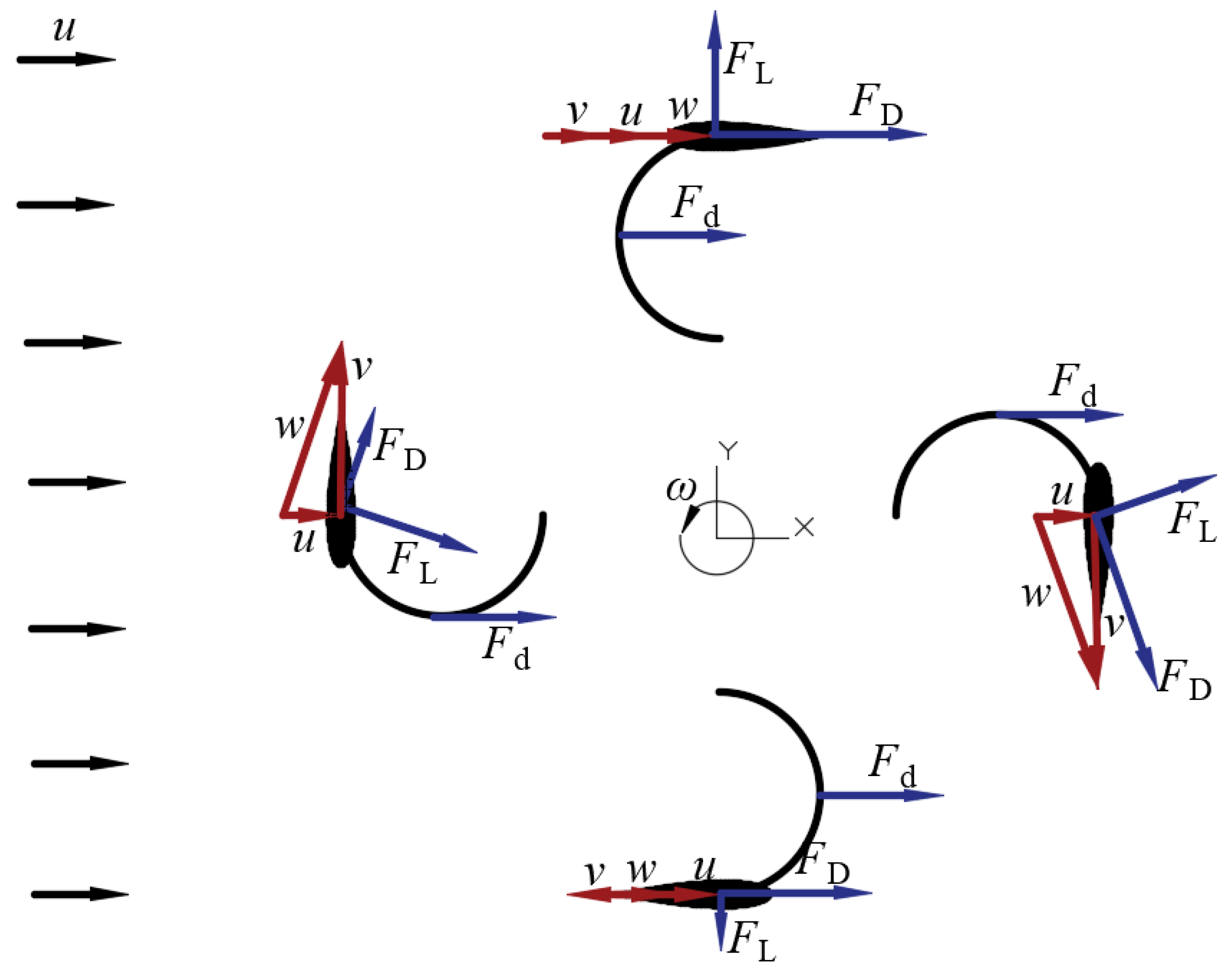
2. Lift-Drag Combined Theory

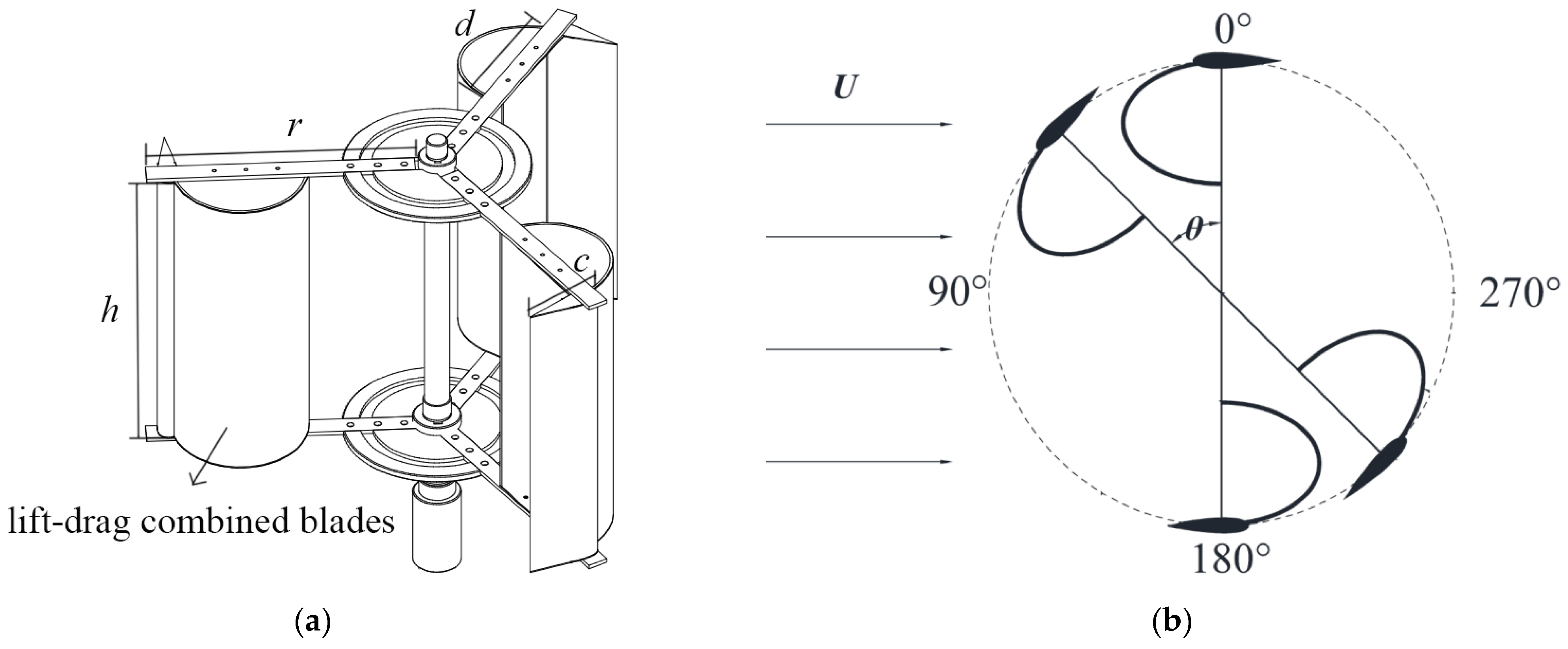
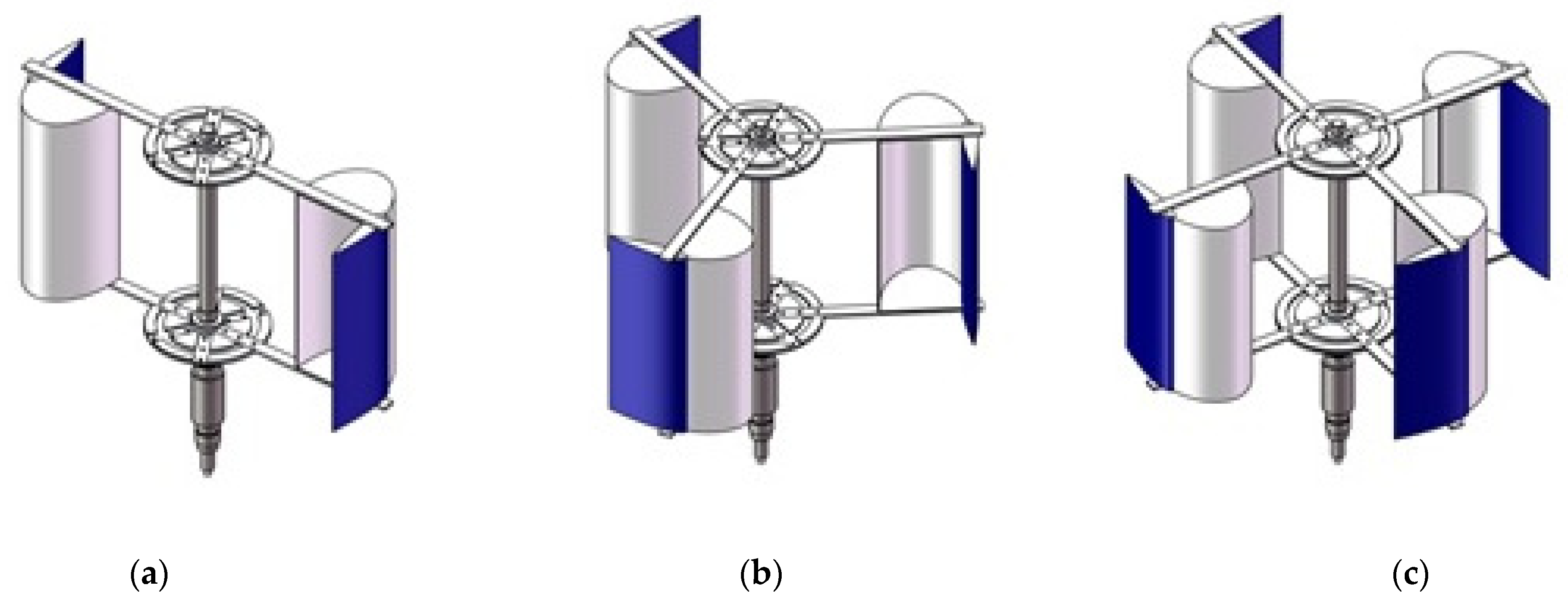
The force analysis on one rotation of a lift-drag combined blade of an LDCS is shown in Figure 1. Where u is the incoming wind speed; v is the relative wind speed; w is the rotational angular velocity of the LDCS; F_L denotes the blade lift; F_D is the blade drag; F_d is the drag of the resistance blade. When the chord is set to be parallel to the incoming flow, the azimuth angle is 0°, the angle that the blade deviates from the 0° position after an anticlockwise rotation is defined as the azimuth angle θ. It can be noted from Figure 1 that drag forms on the drag blade during one rotation of a lift-drag combined blade of an LDCS when incoming flow passes through it. The drag force is larger at 0° and 180°, the maximum occurs at 180°. The moments are quite small at 90° and 270°. When the incoming flow passes through a lift blade, aerodynamic lift is formed, and the moment produced by aerodynamic force is characterized by periodic changes. The moments are small 0° and 180°, and large at 90° and 270°. The moment variations of drag and lift blades are periodic and complementary; thus, a large aerodynamic moment can always be generated during one rotation of the lift-drag combined blade, which plays an important role in the static characteristics of the LDCS.

Figure 2 shows the flow field of the lift-drag combined blades of an LDCS. It can be noted that the airflow can not be separated significantly at the trailing edges of the drag blades. This is because the increased lift blades form an angle of attack with the local inflow velocity, the air on both sides flows against the airfoil at the small angle of attack, which relieves the airflow separation at the trailing edges of the drag blades and increases the tangential force of the LDCS. The above results are fundamentally responsible for the excellent static characteristics of the LDCS.

3. Model Design

The LDCS structure models are composed of two, three, and four lift-drag combined blades, respectively. The 3D modeling of the models is shown in Figure 3. A diagram of model structural parameters and rotation azimuth of the LDCS are shown in Figure 4. Model parameters are listed in

Table 1. Structural parameters of LDCS model with three blade numbers.

Parameter Name	Symbol	Value
Opening diameter of lift-drag combined blade	d	150 mm
Height of LDCS	h	300 mm
Rotation radius	r	280 mm
Lift blade airfoil	-	NACA0018
Lift blade chord length	c	100 mm
Number of lift-drag combined blades	n	2, 3, 4
Rotation azimuth	θ	0°–360°

.

4. Research Methods

4.1. Numerical Simulation Methods

The numerical simulation methods have been developed, and numerical simulation costs have been reduced with more accurate model numerical simulation. The numerical simulation speed has been greatly improved during data numerical simulation. The processed images are more beautified, and the numerical simulation results are more credible, which has become one of the main methods for wind turbine performance prediction and design [24,25,26]. ANSYS is a powerful and widely recognized CFD software, being capable of conducting detailed studies to analyze complex and unsteady aerodynamic flows associated with wind turbine operational situations for transient 2D-3D numerical simulation. For the current work, 2D computational fluid dynamics analysis and numerical simulation were performed by using ANSYS Fluent19.0, which has the potential to provide a realistic numerical simulation of the proposed rotor configurations flow field and address flow problems around their complex geometries to obtain a carefully settled and comprehensive study without high cost involved [27,28,29]. This study is mainly to compare the aerodynamic characteristics of the three-blade formats LDCS and the flow field flow mechanism. Therefore, based on the principle of saving time and costs, this study was carried out using two-dimensional numerical simulation.

4.1.1. Governing Equation

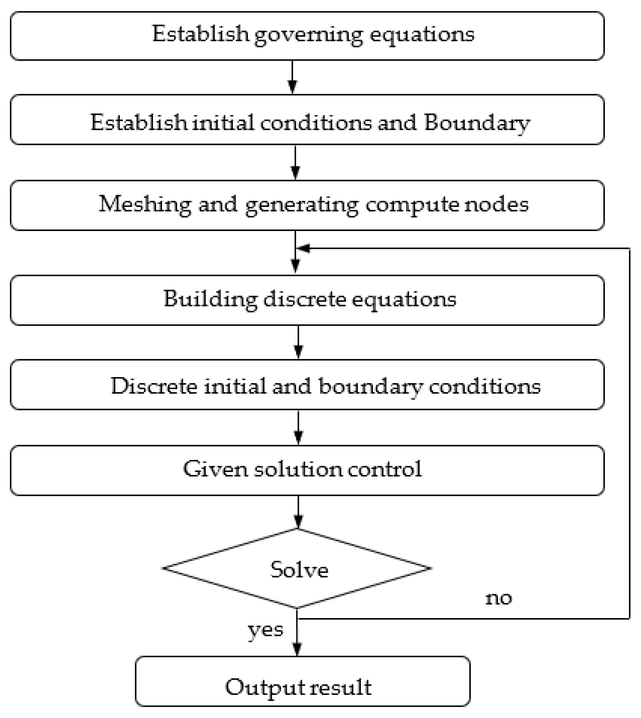
The numerical simulation process in this study used the equation of conservation of mass (1) and the equation of conservation of momentum (2) [30,31].

$$\frac{\partial \overline{U_{\mathrm{i}}}}{\partial x_i}=0$$

(1)

$$\frac{\partial {\overline{U}}_{\mathrm{i}}}{\partial t}+{\overline{U}}_j\frac{\partial {\overline{U}}_i}{\partial x_j}=-\frac{1}{\rho }\frac{\partial \overline{P}}{\partial x_i}+\frac{\partial }{\partial x_j}\left[\left(\nu +{\nu }_T\right)\frac{{\overline{U}}_j}{\partial x_i}\right]$$

(2)

where ρ, ν, and ν_T are the air density, molecular viscosity, and eddy viscosity, respectively.

4.1.2. Workflow

The key steps of numerical simulation mainly include pre-processing, solver settings, and post-processing. The specific workflow of numerical simulation is shown in Figure 5.

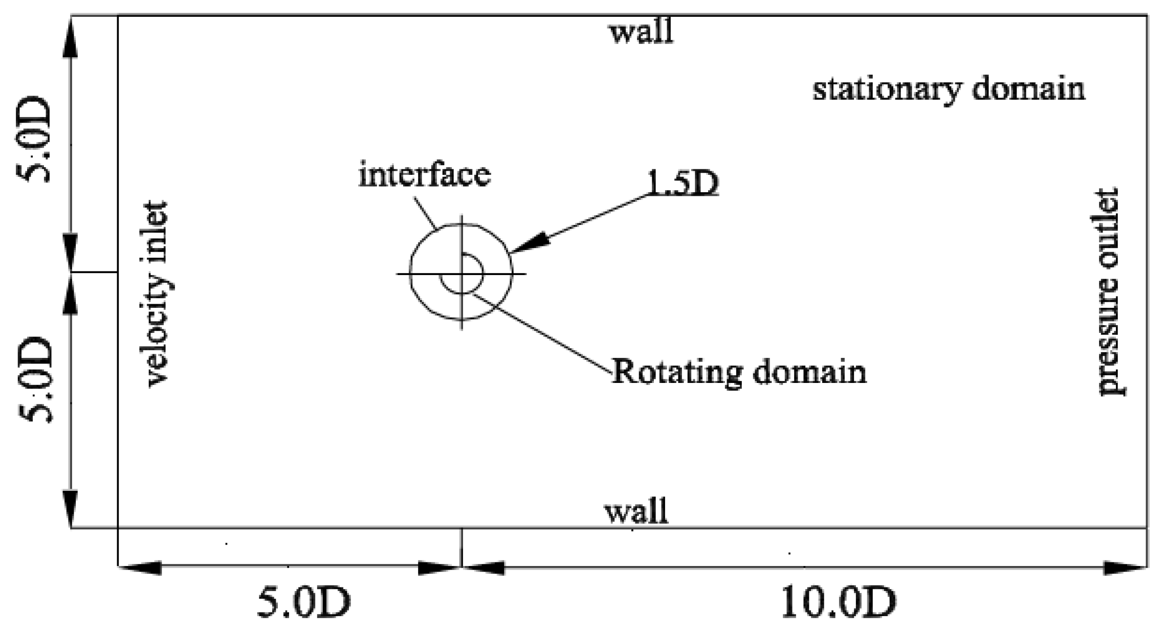
4.1.3. Numerical Simulation Domain Establishment

The selection of the numerical simulation domain size can directly influence the final numerical simulation results; thus, the numerical simulation efficiency should be considered as much as possible while ensuring the numerical simulation accuracy. The research model in this paper was a VAWT with the same axial cross-section so that the numerical simulation model can be simplified to a 2D model. The structure of the LDCS model with little influence on the results was simplified, and bolts, flanges, beams, etc., were removed to establish a numerical simulation model. A computational flow field was established around the computational model. The size of the selected flow field was 10D × 15D. Figure 6 showed the calculated flow field.

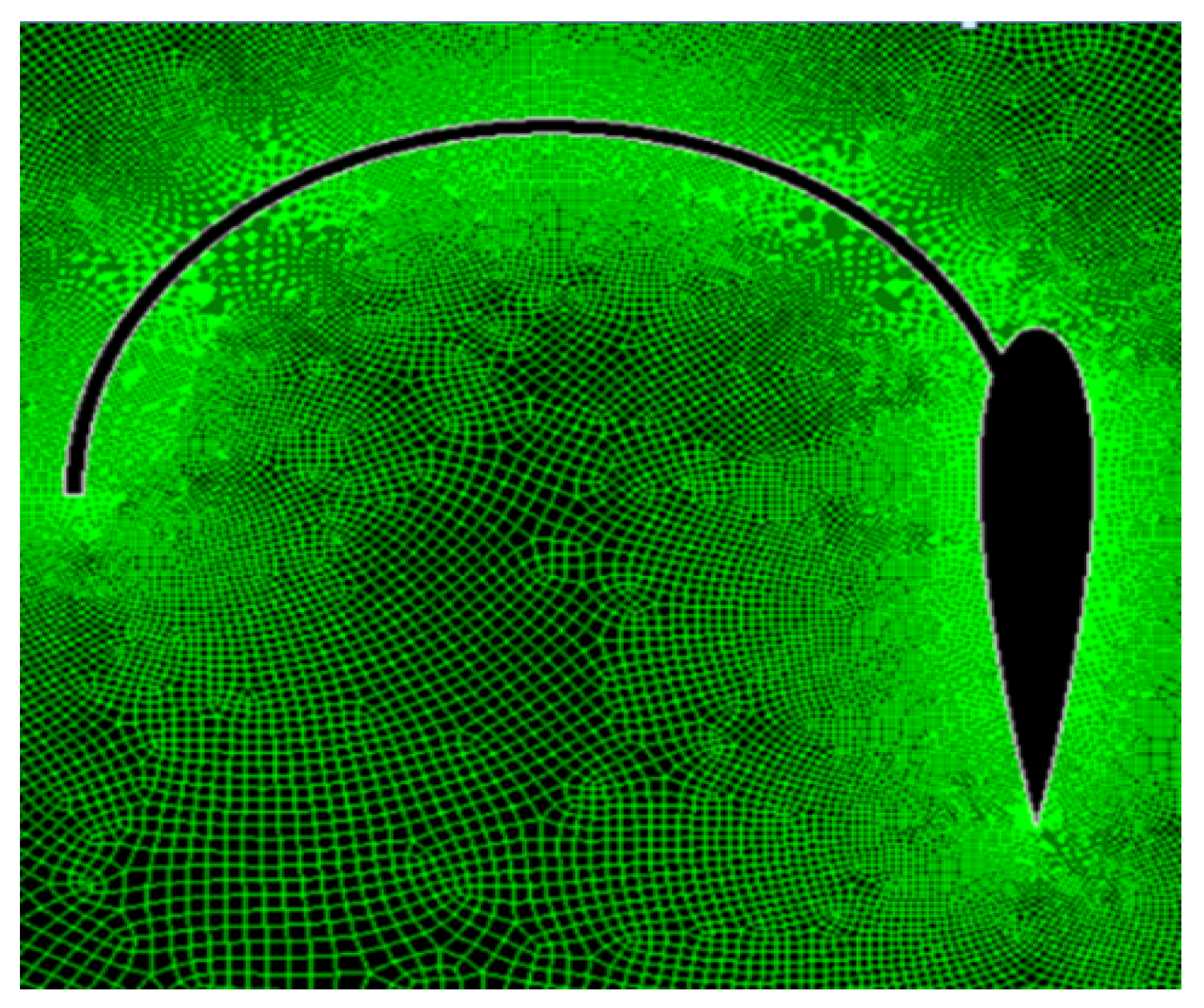
4.1.4. Geometric Meshing

Meshing is an extremely important step in numerical simulation. In order to ensure the accuracy and efficiency of the numerical simulation simultaneously. Combining dynamic and static grids was adopted in the numerical simulation. The area was set swept during the LDCS rotation as a dynamic mesh area and encrypt the mesh in this area. The interface between the dynamic mesh area and the static mesh area was set as a slip surface, which was employed to transfer the energy of the dynamic mesh area and the static mesh area. The shape of the lift blades and the resistance blades was irregular, and the distribution between each grid unit and node was random; thus, an unstructured grid was used in the numerical simulation. Figure 7 shows the meshing of the blades around the lift-drag bladed.

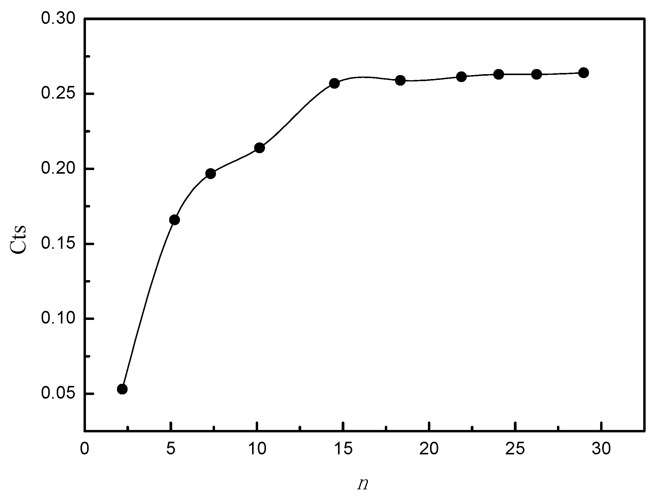
4.1.5. Grid Independence Verification

An appropriate number of grids is the basis to ensure numerical simulation accuracy and reduce numerical simulation time. We first need to perform grid independence verification before numerical simulation. By comparing and analyzing the influence of different grid numbers on the numerical simulation results, a proper number of grids were selected to ensure the rationality of the number of grids. This numerical simulation aimed to verify the grid independence. The static torque coefficient of two-bladed LDCS at 20° azimuths was used to verify the grid independence. As shown in Figure 8, when the number of grids was greater than 220,000, the calculated value tends to be stable; thus, the number from 250,000 to 280,000 grids were selected to conduct a numerical simulation of the static aerodynamic characteristics of LDCS with different blade numbers.

4.1.6. Boundary Conditions and Solutions

The numerical simulation model applied in this paper was incompressible flow. The inlet boundary was calculated, and the inlet velocity was selected. The value was U = 10 m/s. The outlet boundary condition was a pressure outlet, which was equal to the normal atmospheric pressure. The value was P = 1 × 10⁵ Pa. The upper and lower boundaries of the numerical simulation domain were set to the wall surface. Impermeable wall boundaries were used to limit the direction of fluid flow. In the static setting, a pressure-based solver was used under the steady incoming flow. The turbulence model used the double standard equation model of k-ε, and the pressure-velocity coupling used the SIMPLEC algorithm. The residual convergence criterion was set to 1 × 10⁵, using the second-order upswing interpolation, the average value of the output data-stable region was regarded as the result output.

4.1.7. Numerical Simulation Method

The three-bladed LDCS models had a period of 180°, 120°, and 90° during a rotation of 360° around the central axis. For comparative analysis, the azimuth was calculated at intervals of 10°. The static torque coefficients of the three LDCS models with the number of blades as a function of azimuth angle were calculated and performed. The static torque coefficient (C_ts) given in Equation (3) was the ratio of the T to the total torque induced by the incoming flow, which was the evaluated parameter to measure the starting characteristics of LDCS.

$$C_{ts}=\frac{T}{\frac{1}{2}\rho A{U}^{2}R}$$

(3)

where T is the static torque of the LDCS, Nm; ρ denotes density, kg/m³; U is the income velocity, m/s; R is the radius of the rotor, A is the areas of LDCS.

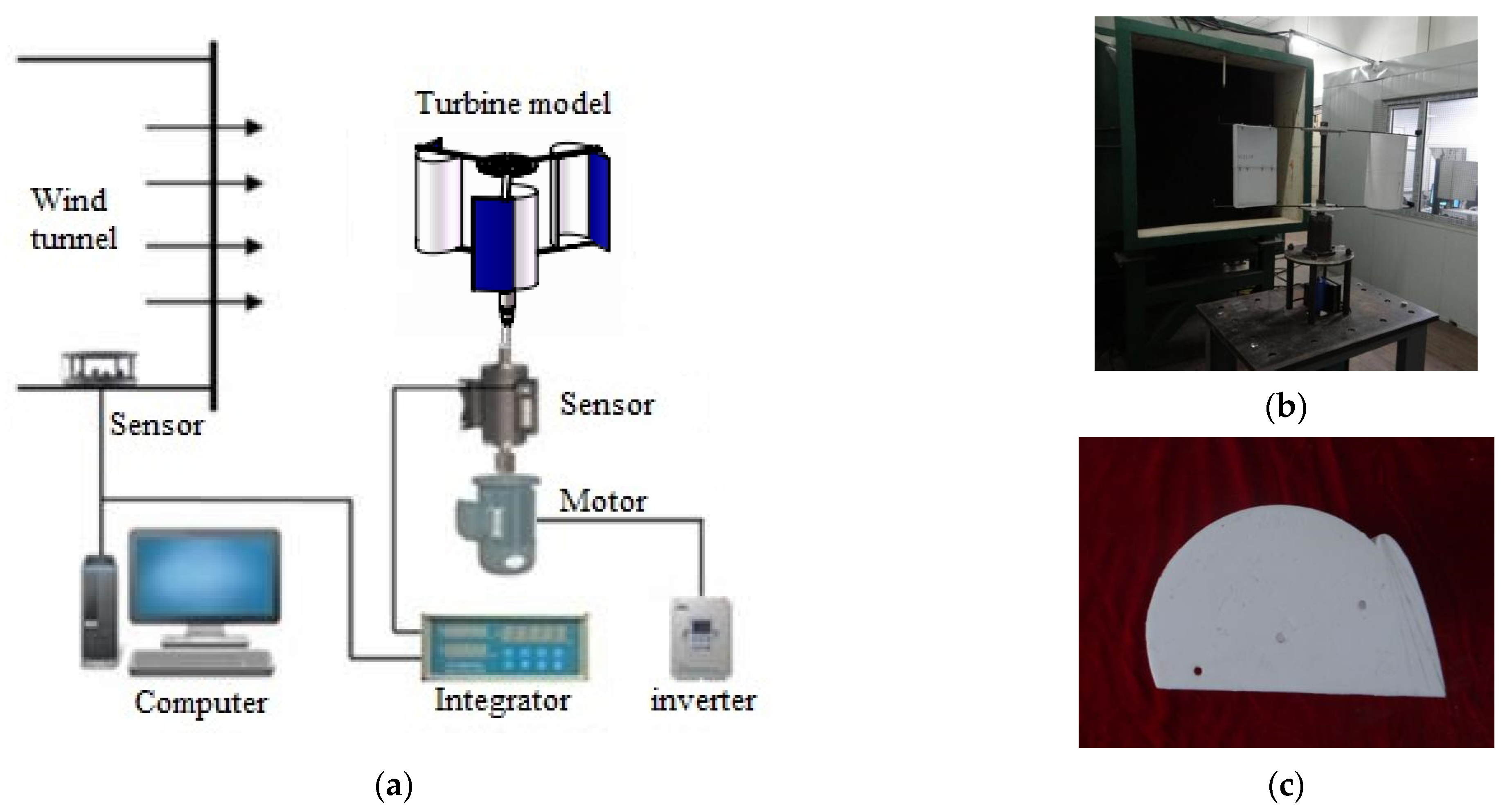
4.2. Wind Tunnel Aerodynamic Performance Test

4.2.1. Wind Tunnel

The wind tunnel tests were conducted using an open jet low-speed wind tunnel. The wind tunnel was 9.1 m long, and the width was 2.3 m, while the test section of the wind tunnel was taken as 1 × 1 m. The range of wind speed supplied by the wind tunnel was 1–20 m/s. The average wind speed precision at the outlet section of the wind tunnel was ±3%. The airflow non-uniformity was <0.5 m/s. The examined rotor was placed at the same height as the center of the wind tunnel outlet and 0.5 m downstream from the outlet. The turbulence intensity is 0.5%, BL thickness is 4.5 mm.

4.2.2. Test Equipment

A wind tunnel test system was established to examine the static aerodynamic characteristics of LDCS. The test equipment parameters and accuracy are shown in

Table 2. Equipment parameters and accuracy table.

Equipment Name	Parameters	Precision
Wind speed sensor	0–50 m/s	±1.0%
Torque sensor	5 Nm	±0.3%
Induction motor	0–2000 rpm	±0.1%
FM	50 Hz	±2.0%

., The static torque test system of LDCS in Figure 9. Figure 9a is the general diagram of the test system, Figure 9b is the actual test model of LDCS, and Figure 9c is the test model of the lift-drag blade, which is made of PLA.

4.2.3. Measurement Method

The test model beam and flanged on the test bench were installed firstly when the LDCS static torque test was performed. The initial azimuth angle was set to be θ = 0°, and the airflow to the wind tunnel U = 6 m/s and U = 10 m/s, respectively. Experiments were then performed at 10° intervals through an angle dial. A period of azimuth rotation was selected. The braking function of the induction motor was used to lock the LDCS to the corresponding azimuth.

4.2.4. Uncertainty Analysis

Two parameters conducted in experiments, including wind speed, and torque have been measured, respectively. Therefore, the transfer formula of relative uncertainty K and standard uncertainty ∆C_ts of C_ts could be obtained as follows:

$$K=\frac{\Delta C_{ts}}{{\overline{C}}_{ts}}=\frac{1}{T}\Delta T+\frac{2}{U}\Delta U$$

(4)

$$\Delta C_{ts}=\overline{C_{ts}}\cdot K$$

(5)

where ∆T and ∆U represent that experimental standard uncertainty of static torque wind speed. According to the transfer formula, the standard uncertainty values of parameters are listed in Table 2.

5. Result Analysis

5.1. Static Characteristics of LDCS of Three Numbers of Blades

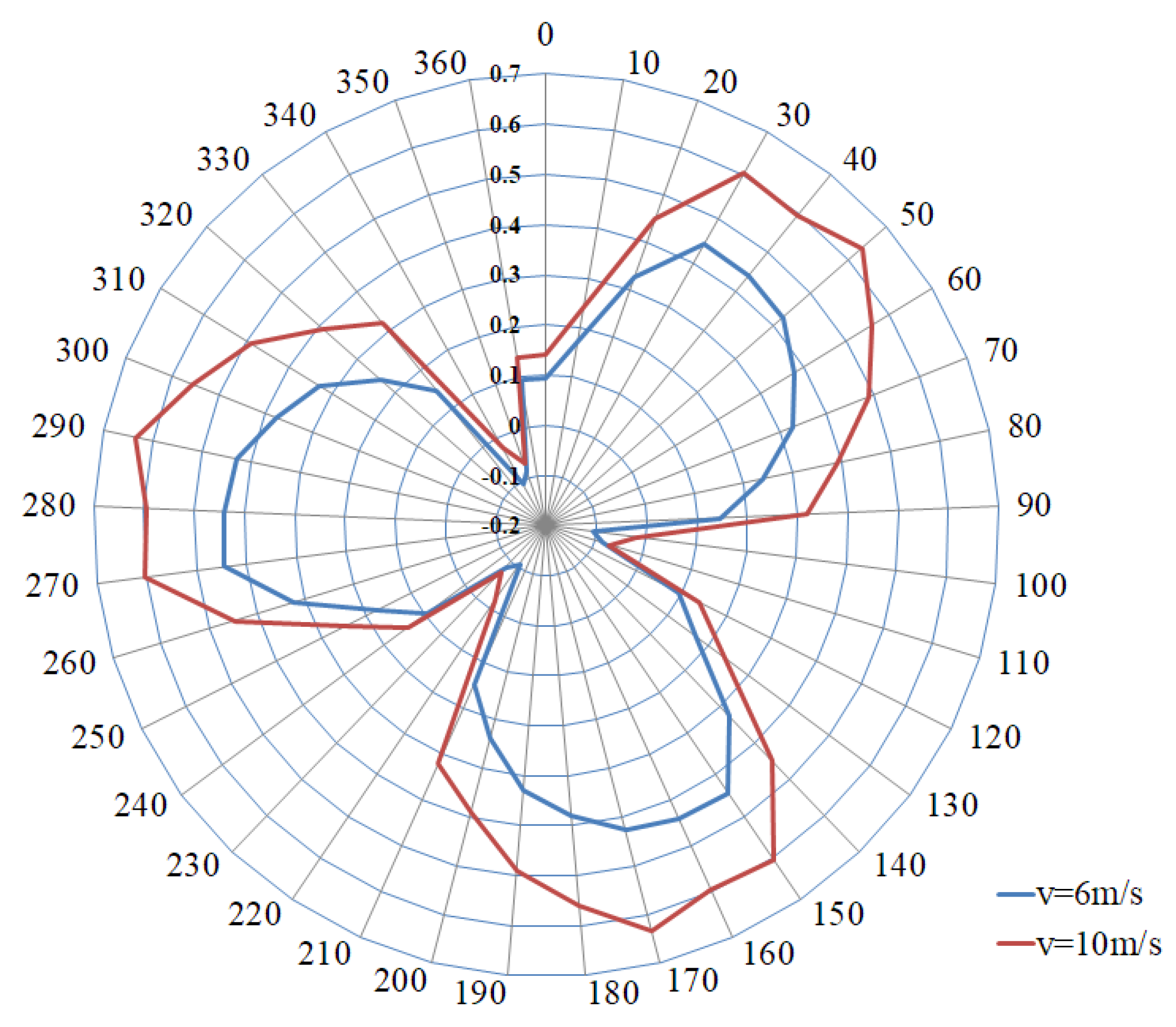
5.1.1. Static Characteristics of Two-Bladed LDCS

Figure 10 showed a radar chart of C_ts variations with azimuth during two periods of two-bladed LDCS rotation at U = 6 m/s and U = 10 m/s wind speed.

It can be noted from Figure 10 that the C_ts of the LDCS fluctuated periodically under both wind speeds, with two peaks and one valley in each period. C_ts peaks were obtained at θ = 50° and θ = 140° during the first rotation cycle when U = 6 m/s, and C_ts-max was appeared at θ = 50° with the value of 0.25. C_ts-min was observed at θ = 120°, which was −0.09. When U = 10 m/s, C_ts peaked at θ = 40° and θ = 140° during the first rotation cycle. The C_ts-max at θ = 40° was 0.39 while the C_ts-min appeared at θ = 120°, which was −0.12. Additionally, it was displayed in Figure 10 that the C_ts change the pattern of LDCS was the same under both wind speeds. Except at θ = 100° and θ = 120°, the C_ts of LDCS were significantly larger at all other angles under U = 10 m/s than those at U = 6 m/s, indicating that the wind speed has an impact on the C_ts of LDCS.

Because the C_ts change pattern for two-bladed LDCS was the same under both wind speeds; however, the static start-up characteristics of LDCS as a starter at low wind speed were more important. Therefore, the velocity and vorticity diagrams are responsible for the occurrence of C_ts-max and C_ts-min at the corresponding azimuth when U = 6 m/s was selected. Figure 11 displayed a cloud magnitude diagram of the velocity magnitude of LDCS when U = 6 m/s, θ = 50° and θ = 120°. Figure 12. showed a cloud magnitude diagram of the vorticity magnitude of LDCS when U = 6 m/s, θ = 50°, and θ = 120°.

It can be observed from Figure 11a that the lift-drag combined upstream blade 1 received air from the convex surface facing the wind when θ = 50°, the velocity of the airflow was high, resulting in a significant high-speed region. Its concave surface was in the leeward region. The airflow flow speed was low, resulting in an extremely low-speed region. Large pressure differences could be generated inside and outside of the blade, thus promoting the increased torque. The concave surface of the lift-drag combined downstream blade 2 received air from the concave surface facing the wind, the airflow flows into the resistance blade, and the speed decreased rapidly to form a low-speed region. The airflow can continue to flow backward along the edges of the downstream blades due to enough space between the two blades, creating a significant high-speed zone. Therefore, a large pressure difference inside and outside the blade was also observed, which promotes the increased torque value at this azimuth.

It can be noted from Figure 11b that the lift-drag combined downstream blade 1 received high-speed airflow when θ = 120°, while the high-speed area was not obvious. Part of the air that flowed on the concave surface flowed along the edges, leading to the increased airflow from the concave surface; thus, the difference in internal and external pressure was reduced, preventing the generation of large torques. The lift-drag combined upstream blade 2 had a convex surface facing the wind and accepted airflow. The airflow velocity was high, and a high-speed area was generated; however, the area was small. There is not much airflow on the concave surface. The airflow speed was reduced, resulting in a low-speed region. Therefore, a pressure difference occurs inside and outside, which promotes the torque at this angle. Through comparing Figure 11a,b, it can be observed in Figure 11a that a large speed difference area was generated around both blades, while in Figure 11b, only the upstream blade 2 generated a small speed difference area. In comparison, the torque that caused the blade to rotate is larger in Figure 11a; thus, the C_ts-max value of the two-bladed LDCS appears when θ = 50°.

From the vorticity diagram in Figure 12, the evolution of the development and extinction of the two-bladed LDCS vortex can be clearly observed. It can be noted by comparing Figure 12a,b that the development area of airflow is obviously different. The vortex area in Figure 12a was significantly larger than that in Figure 12b, and the wake region had separation and shedding vortices, while the development area was shorter, and the energy loss was smaller. In Figure 12a, the concave surfaces of blade 1 and blade 2 were basically in the low-speed region, and the convex surface was in the high-speed region. Therefore, the pressure difference between the inside and outside was large, and a large driving torque was generated. In Figure 12b, the low-velocity region of airflow in the concave surfaces of blade 1 and blade 2 decreased. The air velocity was increased compared with Figure 12a; thus, the pressure difference between the inside and outside was small; meanwhile, the blade pushing torque was also small. This further clarifies why the LDCS had a C-max value at θ = 50° and a C_ts-min value at θ = 120°.

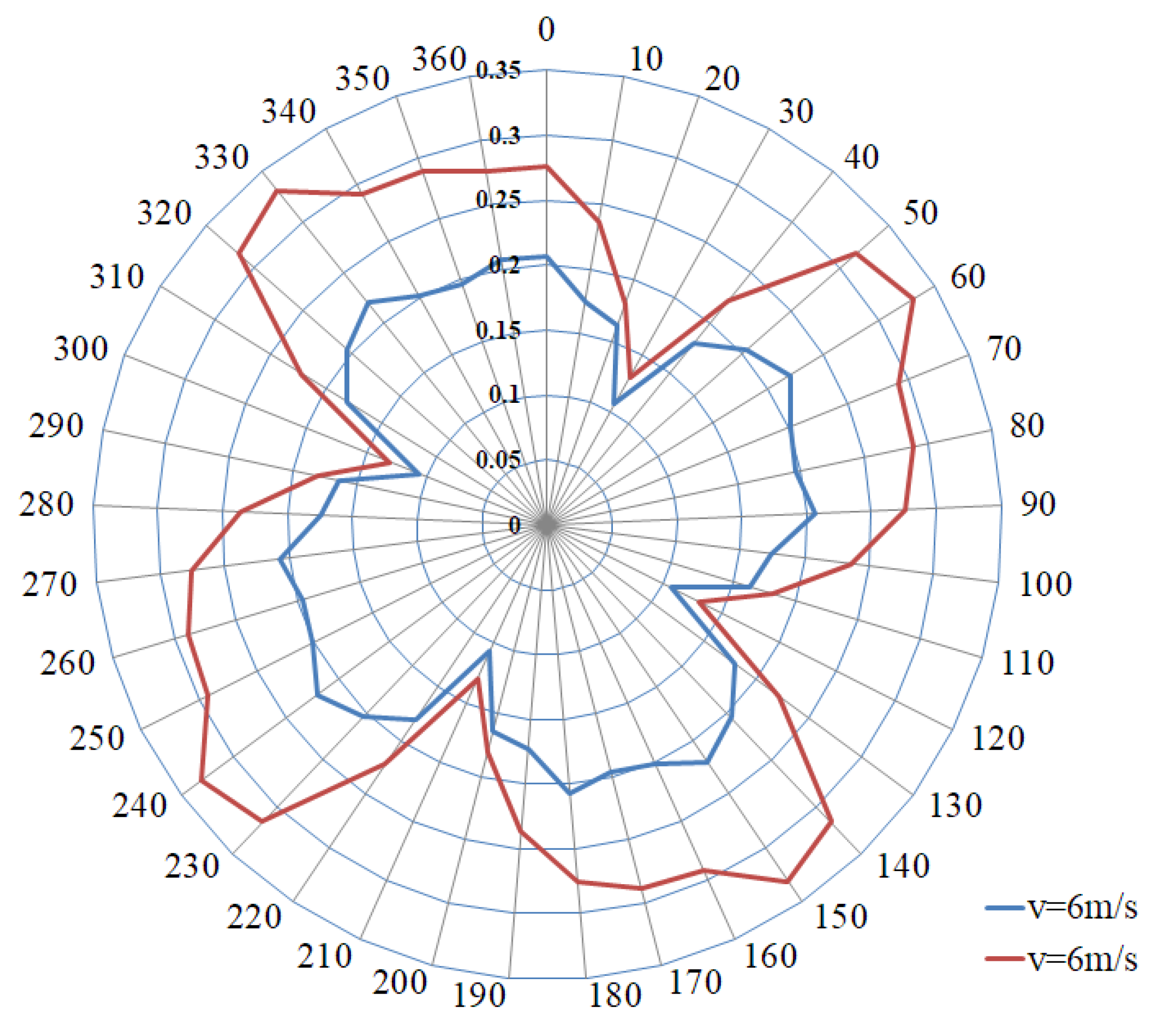
5.1.2. Static Characteristics of Three-Bladed LDCS

Figure 13 shows a radar chart of C_ts as a function of azimuth upon three periods of three-bladed LDCS rotation at U = 6 m/s and U = 10 m/s wind speed.

It can be seen from Figure 13 that the C_ts of the LDCS fluctuated periodically under both wind speeds, and the peak appeared only once per cycle. C_ts reaches a peak at θ = 30° during the first rotation period when U = 6 m/s. At this time, Cts-max was 0.44. C_ts-min appears at θ = 100°, which was -0.11. When U = 10 m/s, C_ts reaches a peak at θ = 50° and C_ts-max is 0.63 during the first rotation cycle. C_ts-min appears at θ = 110°, which was −0.07. In addition, it can be concluded from the comparison in Figure 13 that the C_ts of LDCS was basically the same under the two wind speeds. The C_ts at all angles were obviously larger when LDCS was U = 10 m/s compared with that when U = 6 m/s, indicating that the C_ts of LDCS will increase significantly with the increased wind speed.

Next, the lower wind speed was also selected. The velocity and vorticity diagrams explain the occurrence of C_ts-max and C_ts-min at the corresponding azimuth under U = 6 m/s. Figure 14 displayed a cloud magnitude diagram of the velocity of three-bladed LDCS when U = 6 m/s, θ = 30° and θ = 100°. Figure 15 showed a cloud magnitude diagram of vorticity of three-bladed LDCS when U = 6 m/s, θ = 30° and θ = 100°.

As shown in Figure 14a, the space between the blades was large when θ = 30°, and the three blades had convex parts that received the air coming from the wind. The concave surfaces of the three blades were all in the leeward area. The low airflow flow speed resulted in an extremely low-speed area. Large pressure differences can be achieved inside and outside the blade, thus promoting increased torque. It is worth noting that downstream blade 2 flows along the blade due to the additional lift blade airflow. A significant lift was generated under the influence of the blade aerodynamic characteristics, which further promoted the increased torque at this azimuth. Thus the C_ts-max value of three-bladed LDCS appeared when θ = 30°. It can be observed from Figure 14b that the airflow flow space was reduced when θ = 100°, and the three blades only had the convex surface of the upstream one blade facing the wind, resulting in a high-velocity region, and the three blades had a lower surface velocity. The internal and external pressure difference was small, no large torque was generated. Therefore, the C_ts value of LDCS was very low at this azimuth.

From the vorticity diagram shown in Figure 15, the changes in the growth are also observed clearly, development and disappearance of the vortex at two azimuth angles. Through comparing Figure 15a,b, it can be seen that the development area of airflow flow was completely different. In Figure 15a, the vortex regular research blade was generated, the wake development area was small, negligible shedding vortex was observed, and the energy loss was low. In Figure 15b, a complex vortex was achieved between the three blades, and it apparently fell back. The downstream wake development area of the two blades was significantly longer, leading to the energy loss at this azimuth. Figure 15a shows that the three blades receiving the incoming side were all in the high-speed zone, which was beneficial for generating a large pressure difference, which in turn generates a large driving force rejection. In Figure 15b, only two blades were in the high-speed region; thus, they failed to produce a large pressure difference and thrust rejection. This further clarifies the C_ts-max value of LDCS at θ = 30° and the C_ts-min value at θ = 100°.

5.1.3. Static Characteristics of Four-Bladed LDCS

Figure 16 shows a radar chart of C_ts as a function of azimuth upon four periods of four-bladed LDCS rotation at U = 6 m/s and U = 10 m/s wind speed.

It can be observed from Figure 16 that the C_ts change law of LDCS was basically the same under both wind speeds, and both of them fluctuated periodically. Each cycle appeared a peak value and a valley value. In the first rotation cycle of four-bladed LDCS, C_ts decreased rapidly and then increased was different from two-blade and three-bladed LDCS, and a valley appeared at a lower azimuth angle of 30°, and then θ = 60° Only peaked. C_ts-max was 0.22 under U = 6 m/s; C_ts-max was 0.33 when U = 10 m/s. In addition, the C_ts of LDCS at all angles were significantly greater when U = 10 m/s compared with that when U = 6 m/s, no negative torque occurred. This shows that expect the wind speed affecting the C_ts of LDCS, the increased number of blades also contributes to eliminating the starting azimuth dead zone.

Next, the lower wind speed was also selected. The velocity and vorticity diagrams are responsible for the occurrence of C_ts-max and C_ts-min at the corresponding azimuth when U = 6 m/s. Figure 17 shows a cloud magnitude diagram of the velocity of four-bladed LDCS when U = 6 m/s, θ = 30° and θ = 60°. Figure 18 displays a cloud magnitude diagram of vorticity of four-bladed LDCS when U = 6 m/s, θ = 30° and θ = 60°.

According to Figure 17a, the flow space between the four blades was large when θ = 30°, and the blades 1, 2, and 4 had convex parts facing the wind, receiving air to flow, the airflow velocity was high, resulting in high-speed area. The concave surfaces of the upstream blades 1 and 4 were leeward regions, leading in extremely low-speed regions. The downstream blades 2 and 3 had airflow flowing into their concave surfaces, and the airflow flow increased to form a higher speed region. Therefore, the driving force at this azimuth angle mainly resulted from the large pressure difference between the inside and outside of the upstream blades 1 and 4. The contribution of the downstream blade 2 and 3 is less. It can be noted from Figure 17b that the airflow flow space was also large when θ = 60°. Blades 1, 2, and 4 all have convex portions facing the wind and receive airflow. The airflow velocity was relatively high, resulting in a high-speed region and a larger range. The concave surfaces of the four blades were in an extremely low-speed region; thus, a large pressure difference was achieved inside and outside the four blades, which promoted the increased driving torque at this azimuth. In addition, the airflow flowed along the blade due to an additional lift blade in the downstream blade 2. A significant lift was generated under the influence of the aerodynamic characteristics of the blade, which further promoted the increased torque at this azimuth. This phenomenon did not exist when θ = 30°, thus the C_ts-max value of four-bladed LDCS appears when θ = 60°.

Similarly, the change of vortex growth development and extinction of four-bladed LDCS can be clearly observed in the vorticity diagram of Figure 18. Comparing Figure 18a,b, it can be noted that the development area of airflow flow was different. In Figure 18a, the vortices were regularly generated along the blades. The wake development area was small, and negligible shedding vortices was achieved. A large vortex was generated inside the downstream blade, and a high-speed region was formed, lowering the pressure difference between the inside and the outside of the blade and also reducing the driving torque. In Figure 18b, the vortices were generated regularly along the blades. The wake development area was small, and negligible shedding vortices was achieved.

The inside of the downstream two blades was still a low-speed region. The pressure difference between the inside and outside of the blades was not to be reduced, thus leading to the large driving torque. In addition, the flow separation of the airflow in the downstream blades in Figure 18b is small, and the energy loss is low compared with the middle and downstream blades in Figure 18a. Therefore, the LDCS had a value of C_ts-min at θ = 30° and a value of C_ts-max at θ = 60°.

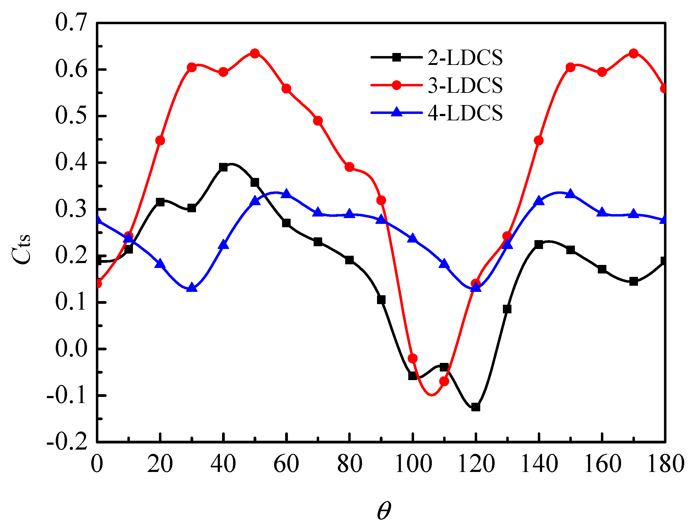
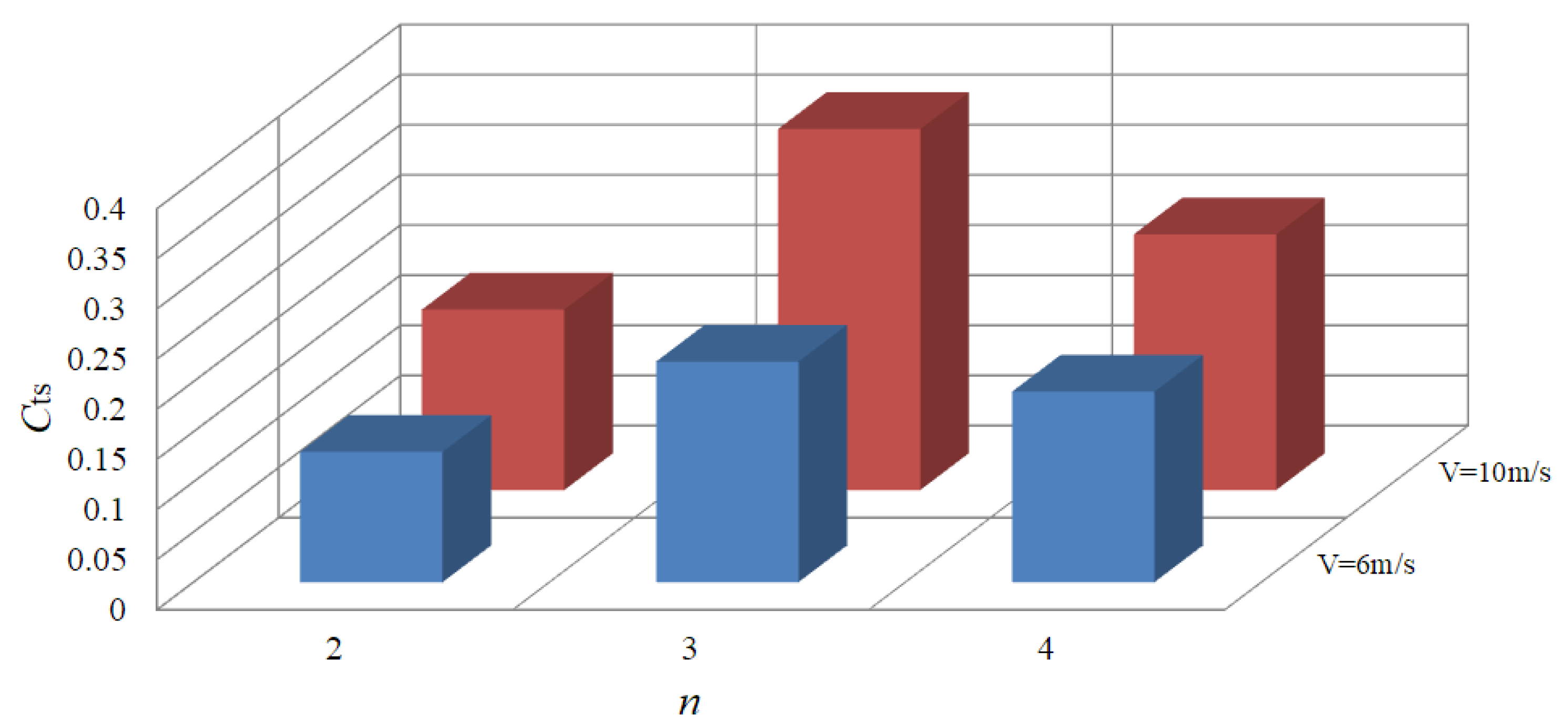
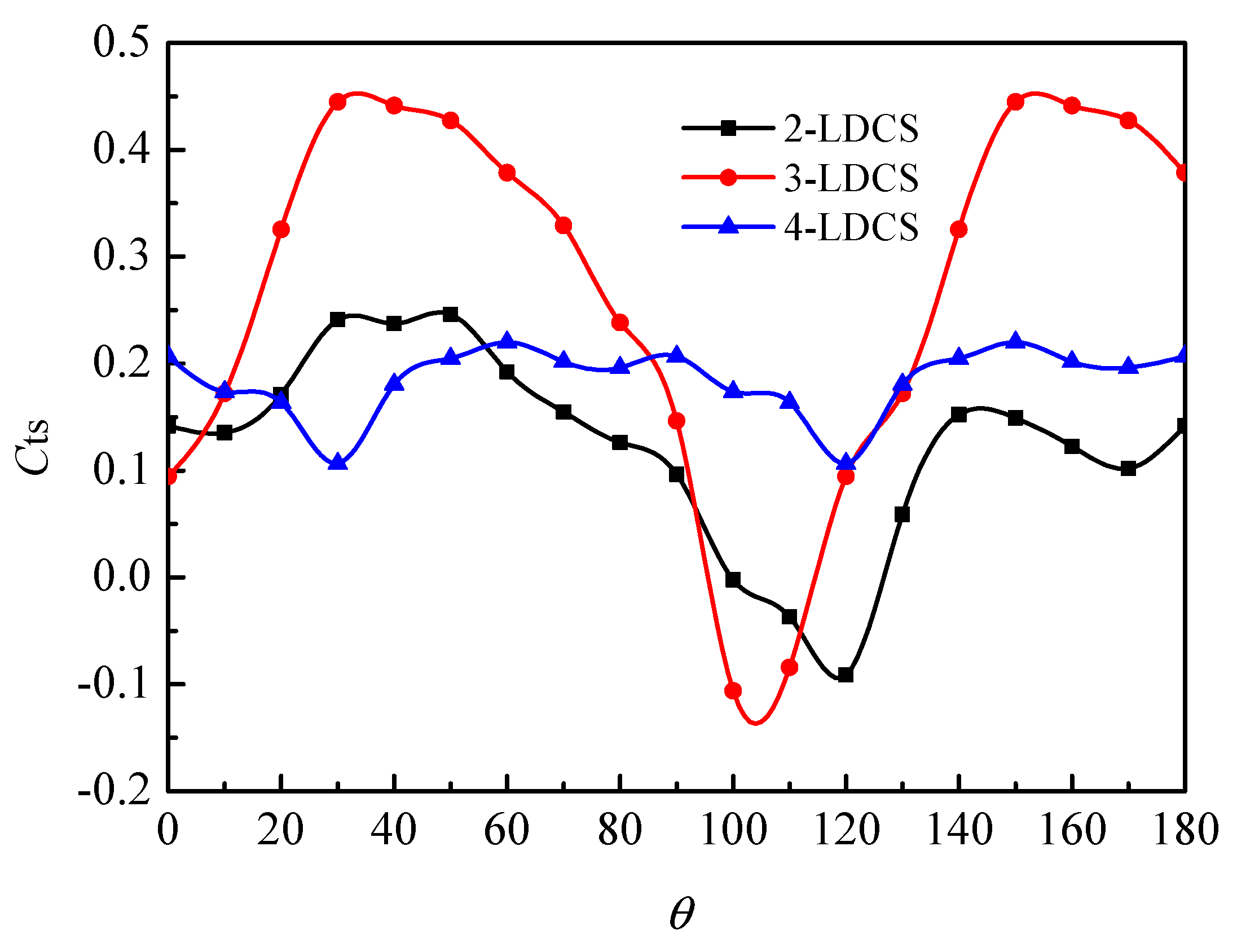
5.2. Comparative Analysis of LDCS Static Characteristics of Three Blade Numbers

Figure 19 and Figure 20 show LDCS static torque coefficients with azimuth angles of three blade numbers in one rotation period at the wind speeds of U = 6 m/s and U = 10 m/s, respectively. Figure 21 displays a histogram of the average increment in the static torque of LDCS for the three blade numbers. The static characteristics of LDCS with three blade numbers can be compared and analyzed through Figure 19, Figure 20 and Figure 21, and the LDCS with the best characteristics is preferably applied to a lift-type VAWT.

As shown in Figure 19, the C_ts of the three numbers of blades LDCS in one rotation period has extremely different distribution rules when U = 6 m/s. Among them, the C_ts of three-bladed LDCS showed a trend of a single high peak and low valley, and the value was higher. The peak at θ = 30° reached around 0.45. The C_ts of two-bladed LDCS showed a double peak and single valley trend with a wide varied range. The C_ts of four-bladed LDCS showed a single peak and single valley change. The four-bladed LDCS had lower C_ts than the two-bladed LDCS. The difference between peak and valley values was small. The C_ts peak of two-bladed LDCS can reach 0.25 at θ = 30°, and the C_ts peak of four-bladed LDCS can reach 0.22 at θ = 60°. It can be observed that the C_ts of LDCS with two-bladed LDCS and three-bladed LDCS were much smaller than the C_ts value of three-bladed LDCS with 0.45. One week’s average solution of the C_ts of three numbers of LDCS can be obtained, with two-blade of 0.13, three-blade of 0.22, and four-blade of 0.19. The average C_ts of three-bladed LDCS was also found to be the highest. Therefore, the static starting characteristics of three-bladed LDCS are best at lower wind speeds.

However, the lowest value of C_ts of three-bladed LDCS was -0.15 in the range of 100°–110°, which indicates that a starting negative torque region for three-bladed LDCS existed, which was smaller than the starting negative torque region of two-bladed LDCS 100°–130°. This was not the case for four-bladed LDCS. This showed that the static torque became more stable as the number of LDCS blades increased. However, from the average of C_ts of two-, three-, and four-bladed LDCS, three-bladed LDCS exhibited the best aerodynamic characteristics.

As shown in Figure 20, the distribution of C_ts of the three numbers of blades LDCS in one rotation period is basically the same as that in Figure 19 when U = 10 m/s; however, the distribution rules between them are completely different. The C_ts of two-bladed LDCS showed a double-peak trend. The C_ts of three-bladed LDCS showed a trend of a single high peak and low valley. The value was higher, reaching a peak of 0.65 at θ = 50°. The C_ts of four-bladed LDCS showed a peak and a valley value. The C_ts of four-bladed LDCS increased compared with the two-bladed LDCS. The difference between the peak and valley values was small. The C_ts peak value of two-bladed LDCS can reach 0.41 at θ = 40°, and the C_ts peak value of four-bladed LDCS can reach 0.35 at θ = 60°. One week’s average torque coefficient was addressed for the three, 0.18 of two blades, 0.36 of three blades, and 0.26 of four blades can be obtained. It can also be seen that the average C_ts of three-bladed LDCS was the highest. In addition, the three-bladed LDCS had a negative starting torque zone in the range of 100°–110°, but this area was smaller than the two-blade starting negative torque zone of 100°–130°. The C_ts of four-bladed LDCS did not exist, which also showed that the static torque becomes more stable as the number of LDCS blades increases.

The average increment in C_ts of the three numbers of blades LDCS was compared between when U = 6 m/s and U = 10 m/s, as shown in Figure 21. It can be further noted that the increased incoming wind speed enabled the LDCS static torquestatic torque average. The value also increased significantly. The increment of C_ts in three-bladed LDCS was the largest. From the average of C_ts of two-, three-, and four-bladed LDCS, the average of C_ts of three-bladed LDCS was the highest. Therefore, the static starting characteristics of three-bladed LDCS were the best under higher wind speeds.

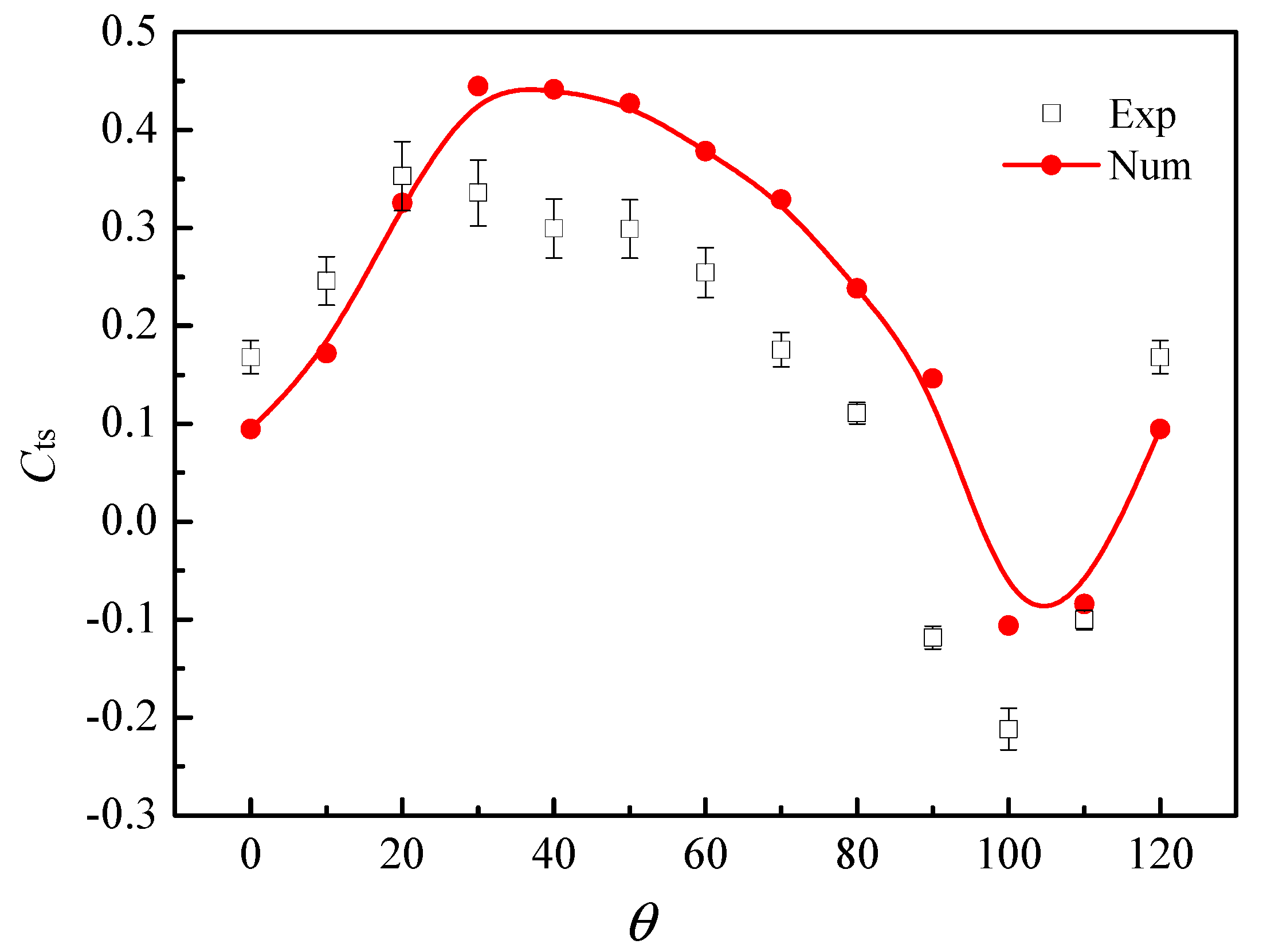
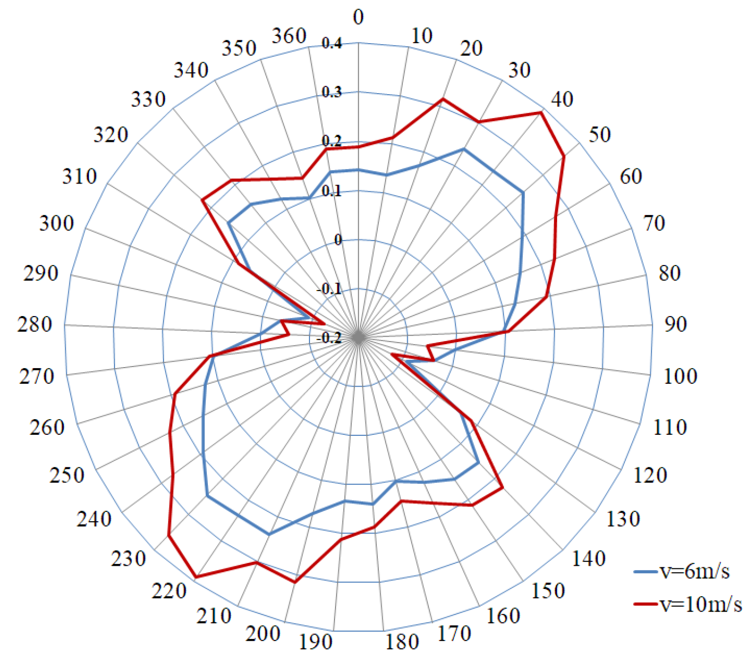
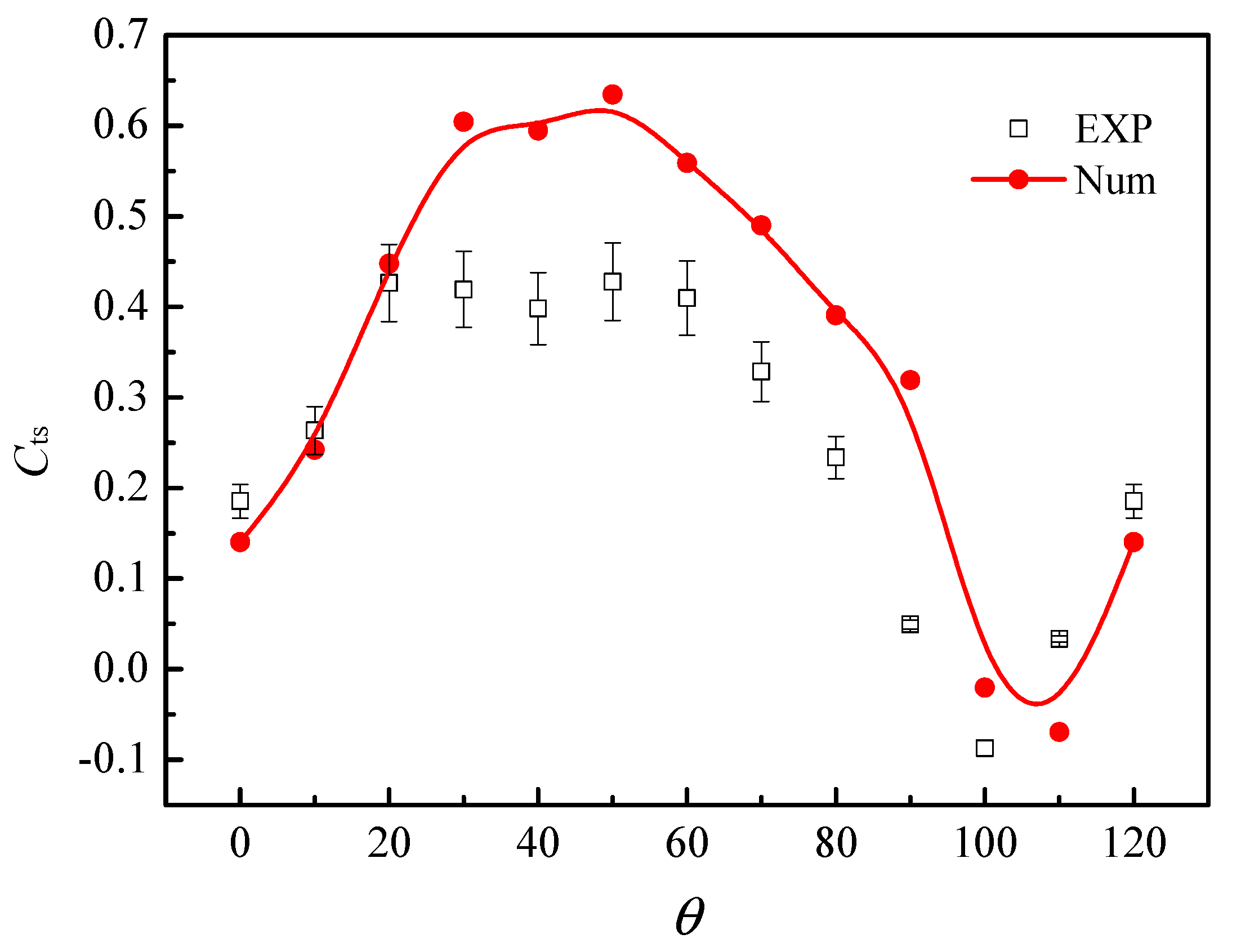
5.3. Wind Tunnel Test Verification

Wind tunnel examinations were performed to verify the C_ts of three-bladed LDCS with the best static starting characteristics as a function of azimuth. The test conditions were consistent with the numerical simulation conditions. The comparison curves between the numerical simulation and the wind tunnel test results are shown in Figure 22 and Figure 23.

The calculated results of the C_ts of the three-bladed LDCS at a wind speed and the wind tunnel test results showed the same fluctuation trend at this wind speed as shown in Figure 22, but results of the numerical simulation and the wind tunnel test were numerically different. The test value was extremely lower. The numerical simulation results of three-bladed LDCS gradually increased under 0°–30°. Around 30°, the C_ts of three-bladed LDCS reached a maximum value of 0.45. The C_ts began to gradually decrease after θ > 30°. At 0°–20°, the wind tunnel test results of three-bladed LDCS gradually increased. The maximum C_ts of three-bladed LDCS was 0.35 when θ = 20°. After θ > 20°, the C_ts of three-bladed LDCS began to gradually decrease. The C_ts of the three-bladed LDCS was reduced to the minimum value, and the calculated value is −0.11, and the wind tunnel test value is −0.21 under the condition of θ = 100°. The calculated value of the average torque coefficient of a three-bladed LDCS rotation was 0.22. The tunnel test value is 0.15, and the difference is only 0.07. It can be noted that the numerical simulation had a smaller error than the wind tunnel test result.

As shown in Figure 23, the numerical simulation result of the C_ts value of the three-bladed LDCS for one period under the incoming wind speed of U = 10 m/s, the wind tunnel test also showed the same fluctuation trend with more consistency. This was mainly due to the fact that the support structure of bearings and beams did not increase the C_ts of LDCS at higher wind speeds compared with low wind speeds. The numerical simulation of three-bladed LDCS C_ts and wind tunnel tests still had a gap in value, and the wind tunnel test values were significantly lower. The numerical simulation results of three-bladed LDCS gradually increased in the θ range of 0°–30°. The C_ts of three-bladed LDCS reached a maximum value of 0.60 when θ was around 30°–50°. In the 30°–50° interval, the plateau period of C_ts appeared with a basically unchanged value. After θ > 50°, the C_ts of three-bladed LDCS began to decrease rapidly. The C_ts wind tunnel test results of three-bladed LDCS gradually increased in the θ range of 0°–20°. When θ = 20°, the maximum wind tunnel test was 0.45. The plateau period of C_ts appeared with a basically unchanged value in the 20°–50° interval. After θ > 50°, wind tunnel test results began to be decreased more rapidly. When θ = 100°, the C_ts wind tunnel test results of three-bladed LDCS dropped to a minimum value of −0.09. When θ = 110°, the numerical simulation result also decreased to a minimum value of −0.07. The average value of C_ts of three-bladed LDCS in a period was 0.34, with the wind tunnel test value of 0.25 and the difference of only 0.09. It can be noted that the error of the numerical simulation was smaller than that of the wind tunnel test.

In short, the comparisons of the wind tunnel tests and numerical simulation in Figure 22 and Figure 23 showed that the numerical simulation in the paper could reflect the aerodynamic characteristics of the three numbers of blades LDCS. The difference between the wind tunnel test and the numerical simulation results was small, mainly resulting from the ignored support structures such as bearings and beams in the numerical simulation; thus, the numerical simulation method of this study is feasible.

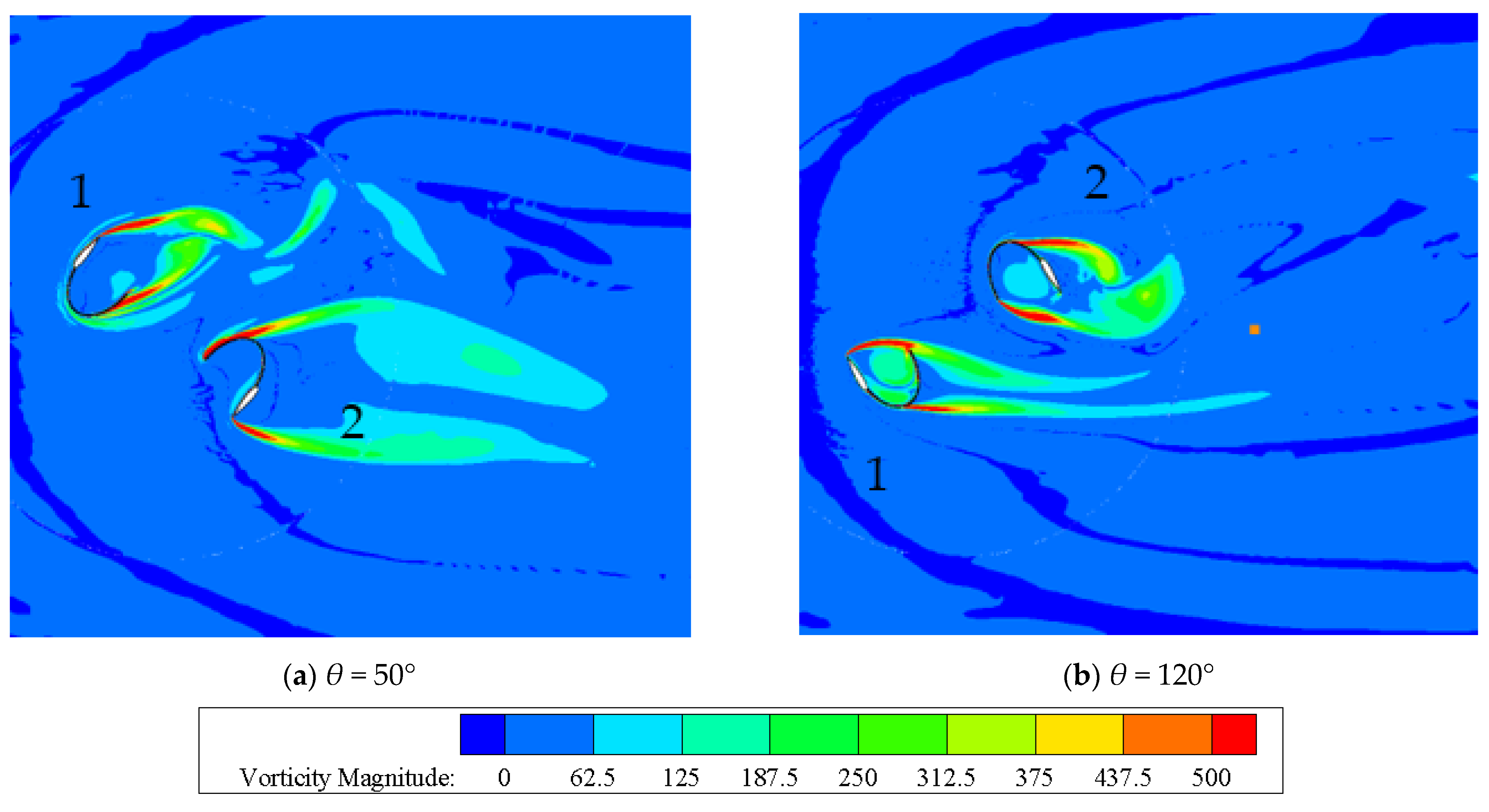
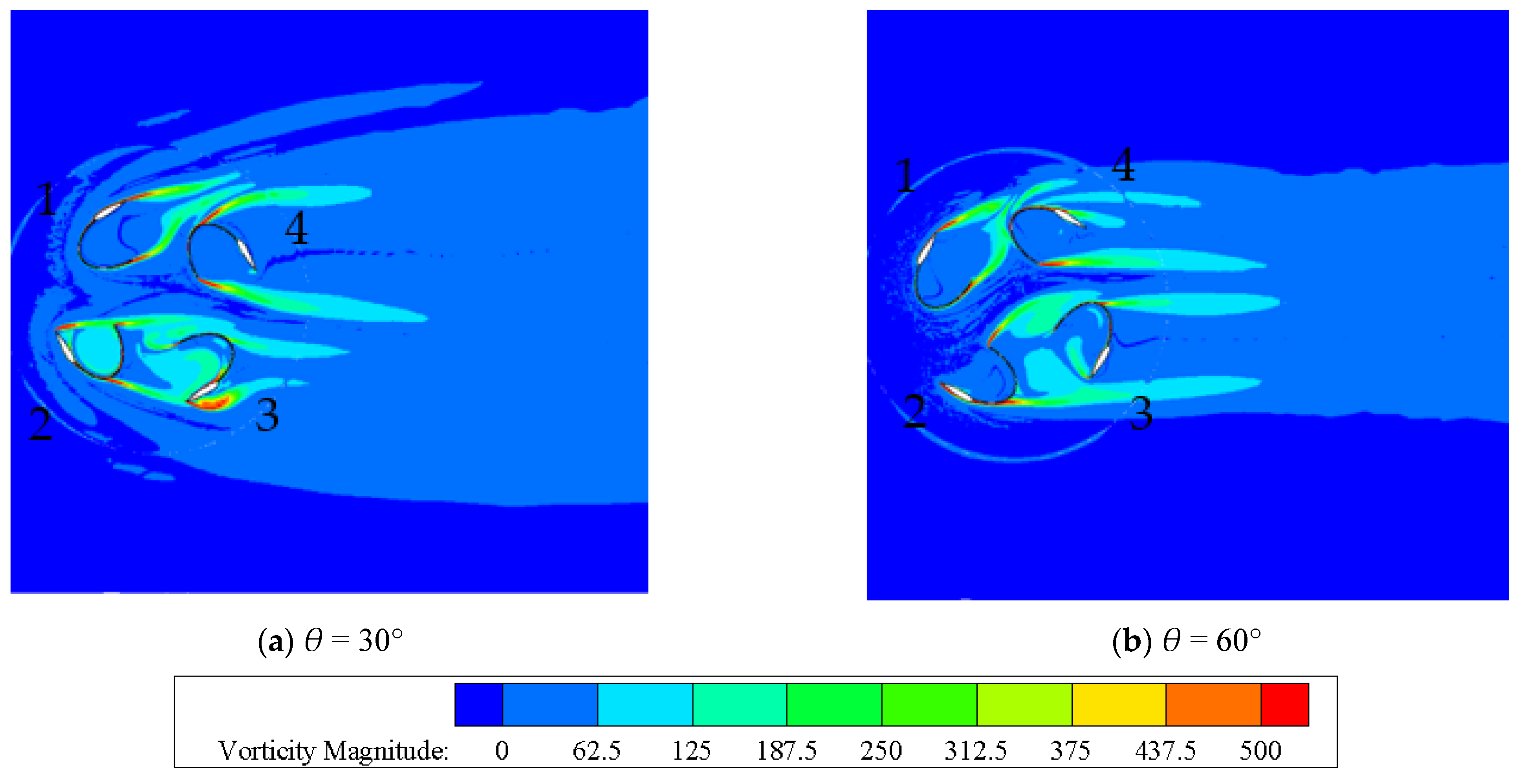
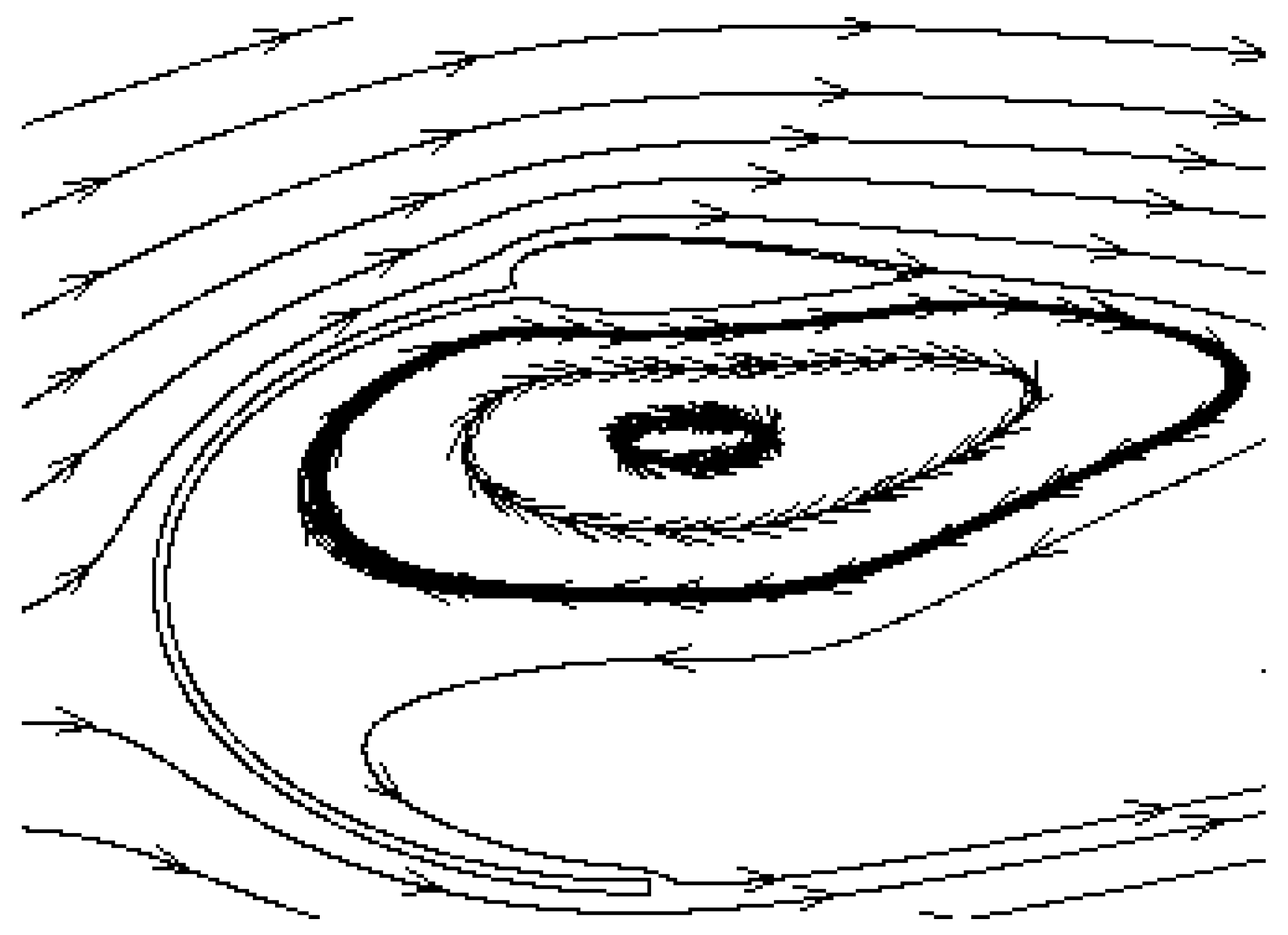
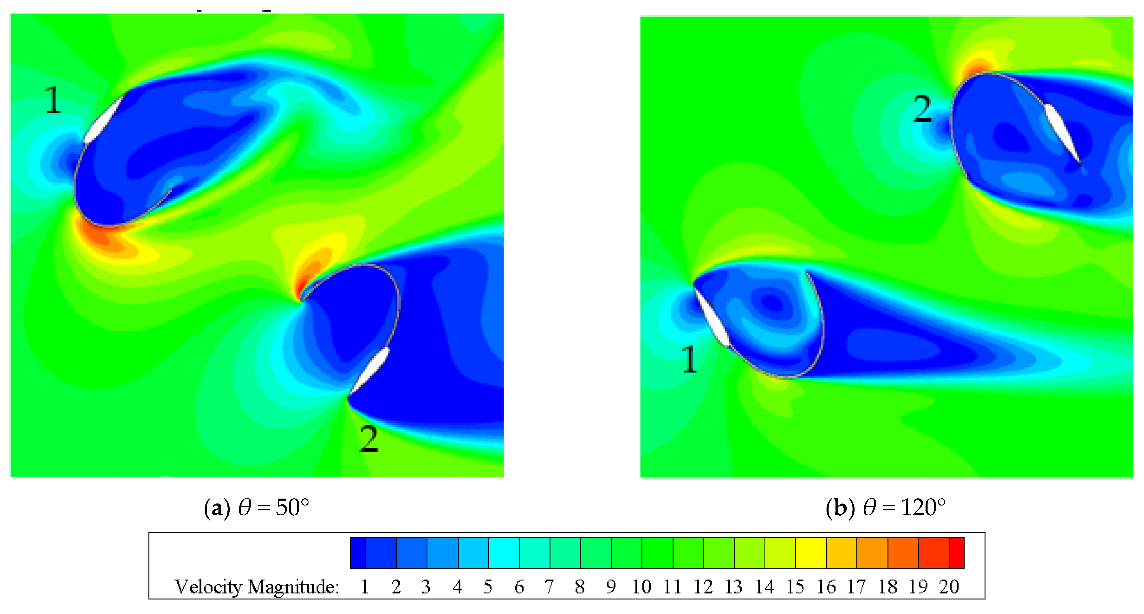
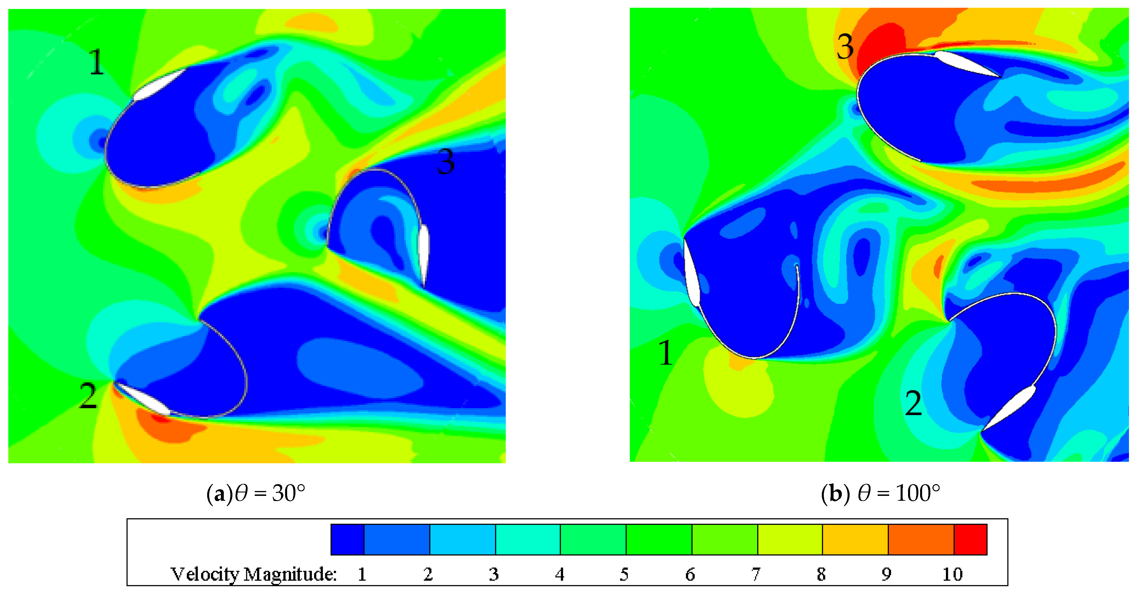
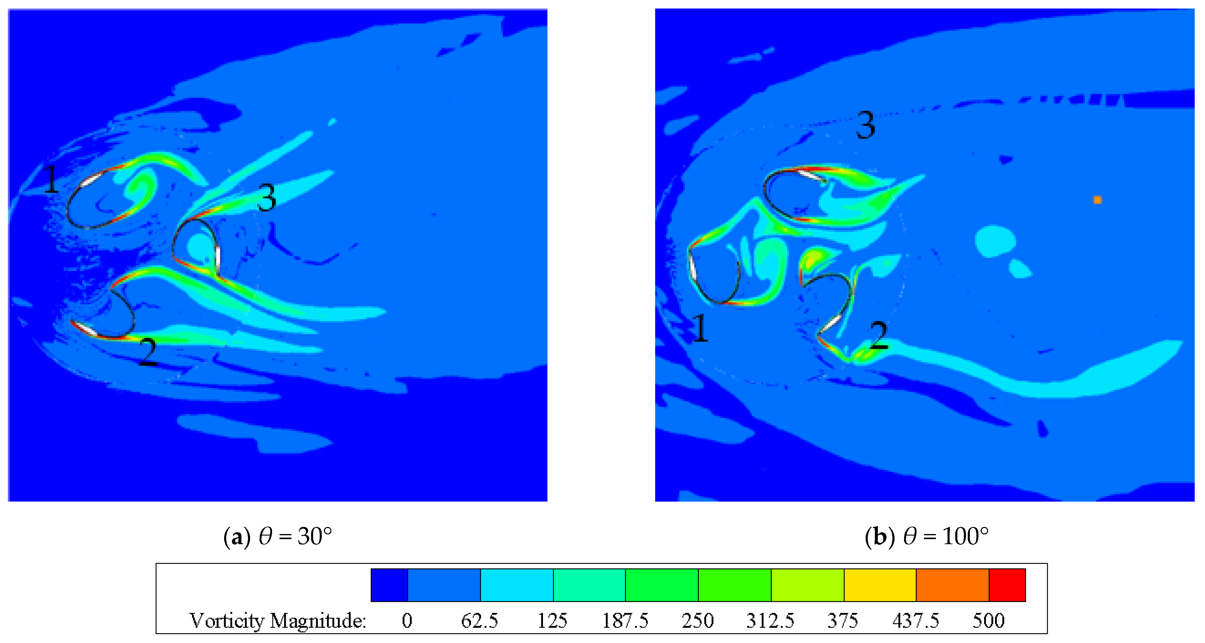
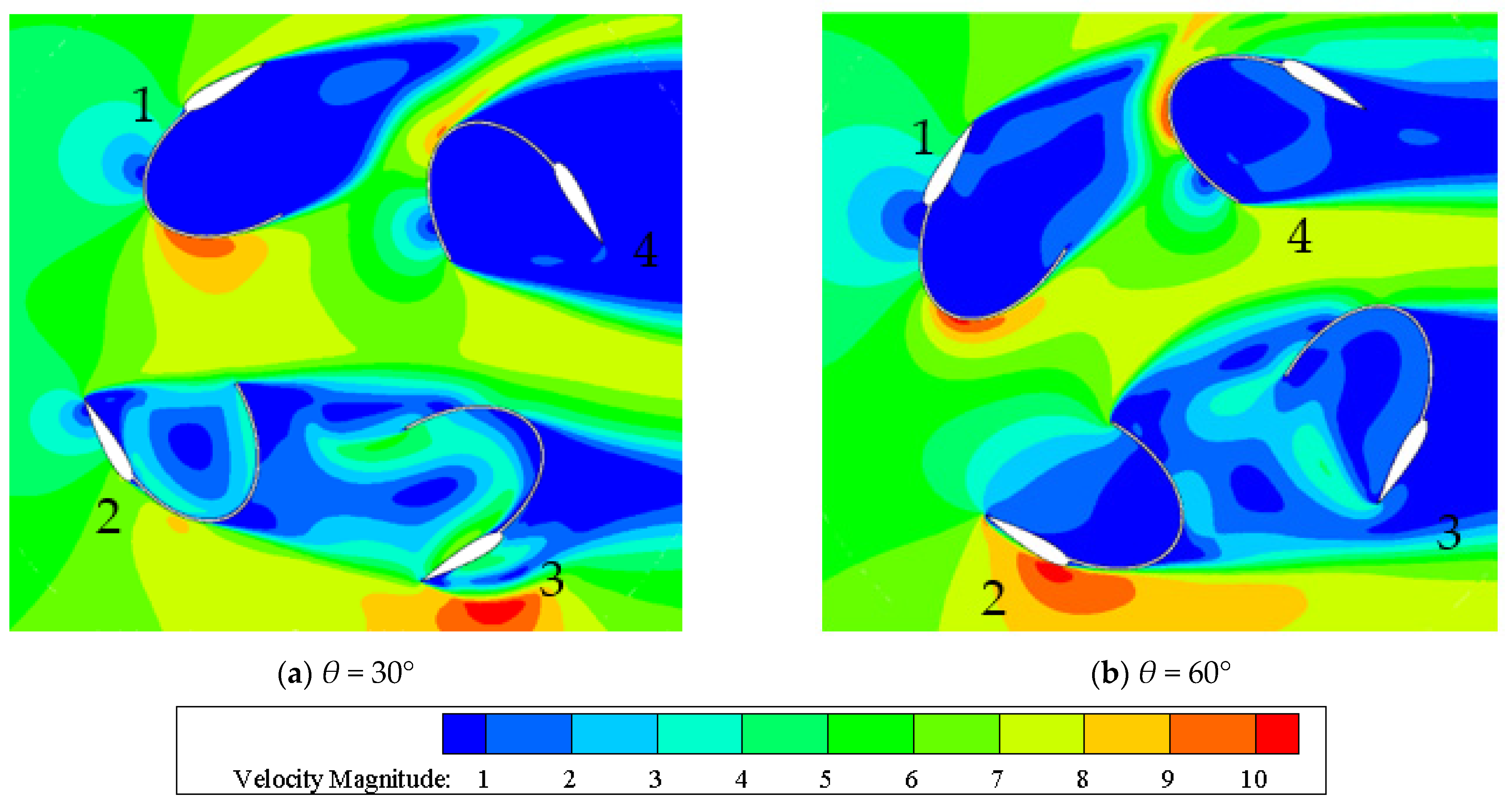
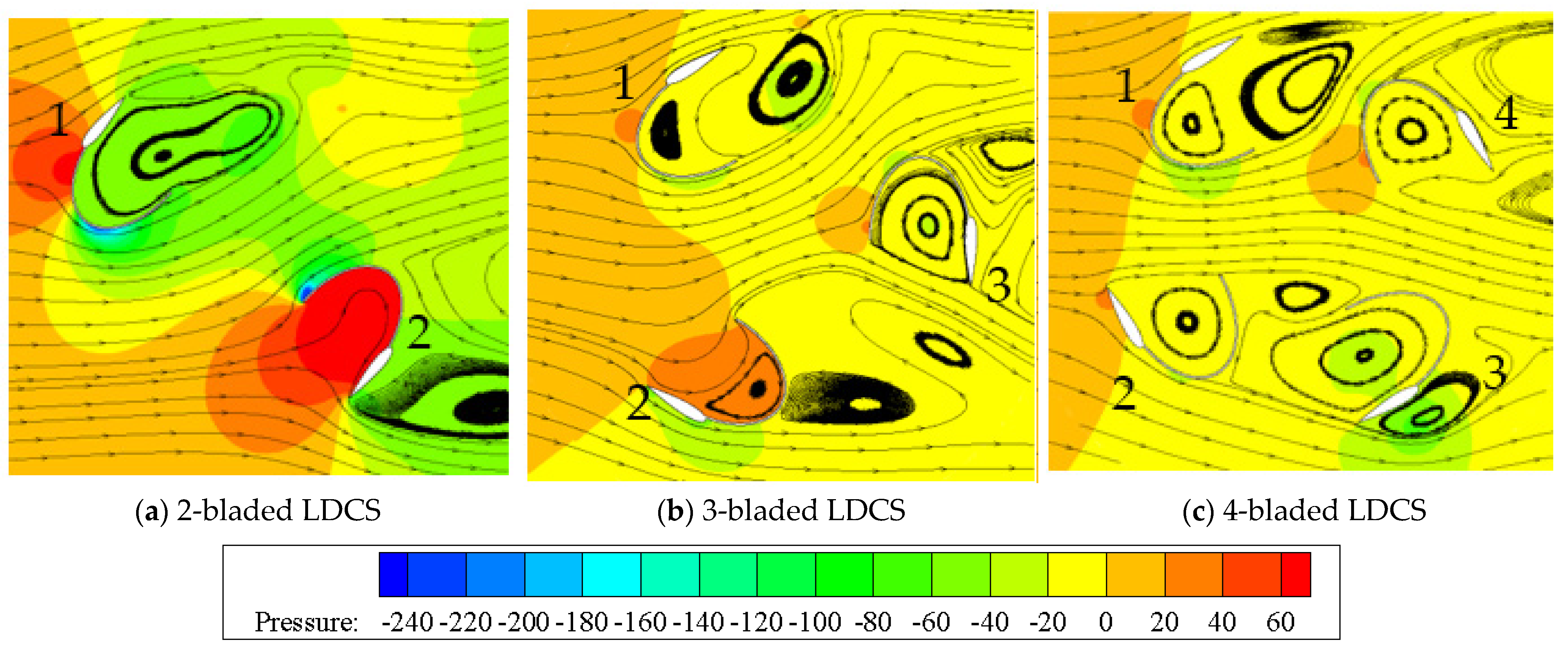
5.4. Comparative Analysis of LDCS Flow Fields with Three Numbers Blades

Through comparing and analyzing the C_ts of LDCS of three numbers of blades at U = 6 m/s and U = 10 m/s, it could be concluded that the obtained starting characteristics of three-bladed LDCS were optimal. In order to explain this conclusion, a comparative analysis was conducted on the flow field of LDCS. LDCS was a lift-drag combined VAWT starter with more important low wind-speed static characteristics. Therefore, the static flow fields of three numbers of blades of LDCS are shown in Figure 24.

It can be observed from Figure 24a that the pressure and streamline distribution around the two-bladed LDCS blades when this azimuth was facing the wind. A positive pressure area appeared on the windward side of the upstream blade 1 and generated a negative torque of LDCS rotation. The concave surface of the downstream blade 2 faced the wind, generating a large positive pressure. The pressure difference between the concave and convex surfaces enabled the blade to receive a large positive torque. It was the main driving force that derived the wind turbine to rotate. Meanwhile, the resistance torque of the upstream blade 1 increased slightly due to the increased lift blade, but a large vortex was generated at the wake of the lift blade. The downstream blade 2 greatly increased the windward area of the LDCS due to the increment of the lifting blades, and the pressure difference between the concave and convex sides of blade 2 was enlarged so that the forward torque to the LDCS of the two blades was greatly increased. However, since the blade 1 was mainly a negative torque, the torque between the two blades to promote the rotation of the LDCS was not large. Therefore, the value was not high, although the LDCS static torque coefficient reached the maximum at this azimuth.

The pressure and streamline distribution around the three-bladed LDCS blades when this azimuth was facing the wind, as shown in Figure 24b. At this time, there were two blades upstream, of which the left blade 1 first faces the wind, and a large positive pressure area was generated on the windward side, inducing a negative torque of LDCS rotation. The concave surface of the downstream blade 2 was facing the wind and generated a large positive pressure. The pressure difference between the concave and convex surfaces caused the blade to receive a large positive torque. At the same time, more air flowed into the blade 2 due to the increased lift blades, which further promoted the increment of the forward aerodynamic torque of the LDCS and expanded the generation of the separation vortex after the blade, resulting in a huge torque difference on both sides of the blade and became the main torque of LDCS rotation at this azimuth. In addition, the right blade 3 was in the gap between the blade 1 and the blade 2; thus, the airflow can still reach the surface of the blade 3 and form a larger positive pressure area. A large vortex was formed inside the blade 3 due to the resistance blade resistance. Torque was also generated. The total positive torque of the three-bladed LDCS was found to be much larger than the total negative torque. The final combined torque derived the LDCS to rotate. Therefore, the three-bladed LDCS had a higher starting torque at this azimuth.

It can be observed from Figure 24c that the pressure and streamline distribution around the four-bladed LDCS blades when this azimuth was facing the wind. There were two blades upstream, of which the left blade 1 first faces the wind, which generated a positive pressure zone on the windward surface and large negative torque. The right blade 4 immediately followed the left blade. A small portion of the upwind airflow flows in, also generating a positive pressure region. A small negative torque was generated inside and outside the blade due to the pressure difference. The downstream blade also had two blades facing the wind. The lift blade of the left blade 3 first faced the wind, which can generate a certain positive torque on both sides of the blade, while the aerodynamic force was not great, and because the convex surface of the left blade first faced the wind to block the airflow, the right side was in a concave position, sufficient airflow through the blades, so that there was not enough forward aerodynamic torque generated. The increment of the lift blade increased the airflow flowing into the blade 3 and promoted the increased forward aerodynamic torque, but it did not produce a great effect due to too large airflow of the left blade 2. Therefore, the aerodynamic difference between the four blades was not large, resulting in a poor starting torque of the four-bladed LDCS.

In short, by comparing the three pressure streamline diagrams in Figure 24a–c, we can clearly find the difference in the flow field after the airflow flows through the three lift-drag combined structures. In comparison, three-bladed LDCS has structural advantages. It has large forward torque and a small reverse torque, driving the LDCS to have a large starting torque; thus, it performs well at low wind speed. Therefore, using it as a starting device can improve the static characteristics of vertical axis wind turbines, which is feasible.

6. Conclusions

Through numerical simulation and wind tunnel tests, the static characteristics of LDCS with two, three, and four blade numbers were compared and analyzed. The following conclusions were as follows:

(1) The change law of C_ts of LDCS of the three types of blades was basically the same under the two wind speeds of U = 6 m/s and U = 10 m/s. The C_ts of LDCS was obviously larger than the angles of all sides under U = 10 m/s. When U = 6 m/s, it indicates that the C_ts of LDCS will increase significantly with the increased wind velocity;

(2) The enhanced incoming wind speed greatly increased the average C_ts of LDCS, the value of the three-bladed LDCS increased the most. The average C_ts of LDCS of the three types of blades shown: when U = 6 m/s, two-blade was 0.13, three-blade was 0.22, four-blade was 0.19. When U = 10 m/s, two-blade was 0.18, three-blade was 0.36 and four-blade was 0.26. Three-lead LDCS had the highest average C_ts, three-bladed LDCS had the best static starting characteristics;

(3) After the airflow flows through the three numbers of blades LDCS, the flow field rules were different. In comparison, three-bladed LDCS possessed structural advantages. A large pressure difference can be generated on both sides of the three blades, resulting in a large forward torque and a small reverse torque, which enabled the LDCS to have a larger starting torque; thus, it performs well at low wind speeds;

(4) At a certain azimuth angle, the lift blade of LDCS has aerodynamic characteristics, which promotes the increase in lift-drag combined blade torque; The flow field of the VAWT rotor starter is improved. Therefore, the LDCS rotor starter has suitable static characteristics and can be used as a starting device.

7. Discussion

The starter is a device to help start the lift-type vertical axis wind turbine. The best operated mode of the starter is to install a control mechanism. When the lift-type vertical axis wind turbine cannot be initiated at low wind speed, start the starter to drive the lift-type VAWT to reach the working speed; When the lift-type VAWT is fully started, the starter can be braked, and the lift-type VAWT can work freely and normally; The starter can be restarted to reduce the speed of the lift-type VAWT under the high speed, which plays a protective role. In this paper, there is no additional control mechanism in the research of starters. Thus, the structure of the combined VAWT should be simplified, and the manufacturing cost of the wind turbine should be reduced in order to reduce the control mechanism of the starter. Therefore, this paper proposes to improve the simple structure of the traditional common resistance starter and design a lift-drag combined starter. The addition of lifting blades of the starter can not only help the starting characteristics of the lift-type vertical axis wind turbine but also reduce the power weakening influence of the starter itself on the lift-type VAWT. Lift-type VAWT can provide full play to its power characteristics under the improved starting characteristics. Of course, the starter’s control mechanism will play a more meaningful role in the working characteristics of the lift-type VAWT and avoid the NACA aircraft being shielded if the starter can take certain measures to stop after the lift-type VAWT is started. The authors will strive to develop new devices in future work to obtain this achievement.

References

1. Rosso-Cerón, A.M.; Kafarov, V. Barriers to social acceptance of renewable energy systems in Colombia. Curr. Opin. Chem. Eng. 2015, 10, 103–110. [Google Scholar] [CrossRef]
2. United Nations General Assembly. Transforming our World: The 2030 Agenda for Sustainable Development. Available online: https://www.unfpa.org/resources/transforming-our-world-2030-agenda-sustainable-development (accessed on 25 September 2015).
3. Zhang, L.; Li, Y.; Zhang, H.; Xu, X.; Yang, Z.; Xu, W. A Review of the potential of district heating system in northern China. Appl. Therm. Eng. 2021, 188, 116605. [Google Scholar] [CrossRef]
4. Fleming, A.; Wise, R.M.; Hansen, H.; Sams, L. The sustainable development goals: A case study. Mar. Policy 2017, 86, 94–103. [Google Scholar] [CrossRef]
5. Paraschivoiu, I. Wind Turbine Design Emphasis on Darrieus Concept; Polytechnic International Press: Montreal, QC, Canada, 2002. [Google Scholar]
6. Miao, W.; Li, C.; Wang, Y.; Xiang, B.; Liu, Q.; Deng, Y. Study of Adaptive Blades in Extreme Environment using Fluid-Structure Interaction Method. J. Fluids Struct. 2019, 91, 102734. [Google Scholar] [CrossRef]
7. Liu, Q.; Miao, W.; Li, C.; Hao, W.; Zhu, H.; Deng, Y. Effects of trailing-edge movable flap on aerodynamic performance and noise characteristics of VAWT. Energy 2019, 189, 116271. [Google Scholar] [CrossRef]
8. Li, Y.; Zhao, S.; Qu, C.; Tong, G.; Feng, F.; Zhao, B.; Kotaro, T. Aerodynamic characteristics of Straight-bladed Vertical Axis Wind Turbine with a curved-outline wind gathering device. Energy Convers. Manag. 2020, 203, 112249. [Google Scholar] [CrossRef]
9. Chen, J.; Yang, H.; Yang, M.; Xu, H.; Hu, Z. A comprehensive review of the theoretical approaches for the airfoil design of lift-type vertical axis wind turbine. Renew. Sustain. Energy Rev. 2015, 51, 1709–1720. [Google Scholar] [CrossRef]
10. Almohammadi, K.M.; Ingham, D.B.; Ma, L.; Pourkashan, M. Computational fluid dynamics (CFD) mesh independency techniques for a straight blade vertical axis wind turbine. Energy 2013, 58, 483–493. [Google Scholar] [CrossRef]
11. Wang, Y.; Sun, X.; Dong, X.; Zhu, B.; Huang, D.; Zheng, Z. Numerical investigation on aerodynamic performance of a novel vertical axis wind turbine with adaptive blades. Energy Convers. Manag. 2016, 108, 275–286. [Google Scholar] [CrossRef]
12. Somoano, M.; Huera-Huarte, F. The effect of blade pitch on the flow dynamics inside the rotor of a three-straight-bladed cross-flow turbine. Proc. Inst. Mech. Eng. Part M J. Eng. Marit. Environ. 2019, 233, 868–878. [Google Scholar] [CrossRef]
13. Santhakumar, S.; Palanivel, I.; Venkatasubramanian, K. A study on the rotational behaviour of a Savonius Wind turbine in low rise highways during different monsoons. Energy Sustain. Dev. 2017, 40, 1–10. [Google Scholar] [CrossRef]
14. Jeon, K.S.; Jeong, J.I.; Pan, J.K.; Ryu, K.W. Effects of end plates with various shapes and sizes on helical Savonius wind turbines. Renew. Energy 2015, 79, 167–176. [Google Scholar] [CrossRef]
15. Driss, Z.; Mlayeh, O.; Driss, D.; Maaloul, M.; Abid, M.S. Numerical calculation and experimental validation of the turbulent flow around a small incurved Savonius wind rotor. Energy 2014, 74, 506–517. [Google Scholar] [CrossRef]
16. Tahani, M.; Rabbani, A.; Kasaeian, A.; Mehrpooya, M.; Mirhosseini, M. Design and numerical investigation of Savonius wind turbine with discharge flow directing capability. Energy 2017, 130, 327–338. [Google Scholar] [CrossRef]
17. El-Baz, A.R.; Youssef, K.; Mohamed, M.H. Innovative improvement of a drag wind turbine performance. Renew. Energy 2015, 86, 89–98. [Google Scholar] [CrossRef]
18. Sahim, K.; Santoso, D.; Puspitasari, D. Investigations on the Effect of Radius Rotor in Combined Darrieus-Savonius Wind Turbine. Int. J. Rotating Mach. 2018, 2018, 1–7. [Google Scholar] [CrossRef] [Green Version]
19. Yanuarsyah, I.; Djanali, V.S.; Dwiyantoro, B.A. Numerical study on a Darrieus-Savonius wind turbine with Darrieus rotor placement variation. In AIP Conference Proceedings; AIP Publishing LLC: Melville, NY, USA, 2018. [Google Scholar]
20. Wakui, T.; Tanzawa, Y.; Hashizume, T.; Nagao, T. Hybrid configuration of Darrieus and Savonius rotors for stand-alone wind turbine-generator systems. Electr. Eng. Jpn. 2005, 150, 13–22. [Google Scholar] [CrossRef]
21. Liang, X.; Fu, S.; Ou, B.; Wu, C.; Chao, C.Y.H.; Pi, K. A computational study of the effects of the radius ratio and attachment angle on the performance of a Darrieus-Savonius combined wind turbine. Renew. Energy 2017, 113, 329–334. [Google Scholar] [CrossRef]
22. Haijie, Z.; Diangui, H.; Guoqing, W. Study of Mutual-Interference between the Blade and the Vortex in the Lift-Drag Type Vertical Axis Wind Turbine. Mach. Des. Manufacture 2014, 1, 76–79. [Google Scholar]
23. Xu, Z.; Huo, Y.L.; Chen, Y.; Yang, H.W.; Tan, H.F. Optimum Design and Study on the Properties of A New Combined Type Vertical Axis Wind Turbine. J. Zhejiang Univ. Technol. 2015, 43, 261–264. [Google Scholar]
24. Alaimo, A.; Esposito, A.; Messineo, A.; Orlando, C.; Tumino, D. 3D CFD analysis of a vertical axis wind turbine. Energies 2015, 8, 3013–3033. [Google Scholar] [CrossRef] [Green Version]
25. Shaheen, M.; El-Sayed, M.; Abdallah, S. Numerical study of two-bucket Savonius wind turbine cluster. J. Wind. Eng. Ind. Aerodyn. 2015, 137, 78–89. [Google Scholar] [CrossRef]
26. Wong, K.H.; Chong, W.T.; Sukiman, N.L.; Shiah, Y.C.; Poh, S.C.; Sopian, K.; Wang, W.C. Experimental and simulation investigation into the effects of a flat plate deflector on vertical axis wind turbine. Energy Convers. Manag. 2018, 160, 109–125. [Google Scholar] [CrossRef]
27. Sarma, N.K.; Biswas, A.; Misra, R.D. Experimental and computational evaluation of Savonius hydrokinetic turbine for low velocity condition with comparison to Savonius wind turbine at the same input power. Energy Convers. Manag. 2014, 83, 88–98. [Google Scholar] [CrossRef]
28. Zhang, L.; Zhu, K.; Zhong, J.; Zhang, L.; Jiang, T.; Li, S.; Zhang, Z. Numerical Investigations of the Effects of the Rotating Shaft and Optimization of Urban Vertical Axis Wind Turbines. Energies 2018, 11, 1870. [Google Scholar] [CrossRef] [Green Version]
29. Zheng, M.; Li, Y.; Tian, Y.; Hu, J.; Zhao, Y.; Yu, L. Effect of blade installation angle on power efficiency of resistance type VAWT by CFD study. Int. J. Energy Environ. Eng. 2015, 6, 1–7. [Google Scholar] [CrossRef] [Green Version]
30. Wilcox, D.C. Turbulence Modeling for CFD; DCW Industries, Inc.: La Canada, CA, USA, 1998. [Google Scholar]
31. Schlichting, H. Boundary-Layer Theory; McGraw-Hill: New York, NY, USA, 1968. [Google Scholar]
Figure 1. Force analysis of LDCS.
Energies 14 06167 g001
Figure 2. Flow field of the lift-drag combine blades of an LDCS.
Energies 14 06167 g002
Figure 3. Three-dimensional modeling of the LDCS model: (a) 2-bladed LDCS; (b) 3-bladed LDCS; (c) 4-bladed LDCS.
Energies 14 06167 g003
Figure 4. Model parameters and rotation azimuth of the LDCS: (a) structural parameter; (b) rotation azimuth.
Energies 14 06167 g004
Figure 5. CFD workflow chart.
Energies 14 06167 g005
Figure 6. Computational domain diagram of wind turbine.
Energies 14 06167 g006
Figure 7. Grid mesh of geometric structure of lift-drag bladed.
Energies 14 06167 g007
Figure 8. Static torque coefficient changed with the number of grids.
Energies 14 06167 g008
Figure 9. Static torque test system of LDCS. (a) General diagram of the test system of LDCS; (b) actual test model of LDCS; (c) test model of the lift-drag bladed.
Energies 14 06167 g009
Figure 10. Radar chart of Cts of 2-bladed LDCS as a function of azimuth.
Energies 14 06167 g010
Figure 11. Velocity magnitude of 2-bladed LDCS (U = 6 m/s): (a) θ = 50°; (b) θ = 120°.
Energies 14 06167 g011
Figure 12. Vorticity magnitude of 2-bladed LDCS (U = 6 m/s): (a) θ = 50°; (b) θ = 120°.
Energies 14 06167 g012
Figure 13. Radar chart of Cts of 3-bladed LDCS as a function of azimuth.
Energies 14 06167 g013
Figure 14. Velocity magnitude of 3-bladed LDCS (U = 6 m/s): (a) θ = 30°: (b) θ = 100°.
Energies 14 06167 g014
Figure 15. Vorticity magnitude of 3-bladed LDCS (U = 6 m/s): (a) θ = 30°; (b) θ = 100°.
Energies 14 06167 g015
Figure 16. Radar chart of Cts of 4-bladed LDCS as a function of azimuth.
Energies 14 06167 g016
Figure 17. Velocity magnitude of 4-bladed LDCS (U = 6 m/s): (a) θ = 30°; (b) θ = 60°.
Energies 14 06167 g017
Figure 18. Vorticity magnitude of 4-bladed LDCS (U = 6 m/s): (a) θ = 50°; (b) θ = 60°.
Energies 14 06167 g018
Figure 19. Curves of LDCS static torque coefficients of three numbers of blades with azimuth angle (U = 6 m/s).
Energies 14 06167 g019
Figure 20. Curves of LDCS static torque coefficients of three numbers of blades with azimuth angle (U = 10 m/s).
Energies 14 06167 g020
Figure 21. The change in the average increase in the static torque of the three numbers of blades LDCS.
Energies 14 06167 g021
Figure 22. Curve of Cts of 3-bladed LDCS as a function of azimuth (U = 6 m/s).
Energies 14 06167 g022
Figure 23. Curve of Cts of 3-bladed LDCS as a function of azimuth (U = 10 m/s).
Energies 14 06167 g023
Figure 24. Static flow fields of three number of bladed LDCS (θ = 30°): (a) 2-bladed LDCS; (b) 3-bladed LDCS; (c) 4-bladed LDCS.
Energies 14 06167 g024