Abstract
An efficient energy management system is integrated with the power grid to collect information about the energy consumption and provide the appropriate control to optimize the supply–demand pattern. Therefore, there is a need for intelligent decisions for the generation and distribution of energy, which is only possible by making the correct future predictions. In the energy market, future knowledge of the energy consumption pattern helps the end-user to decide when to buy or sell the energy to reduce the energy cost and decrease the peak consumption. The Internet of things (IoT) and energy data analytic techniques have provided the convenience to collect the data from the end devices on a large scale and to manipulate all the recorded data. Forecasting an electric load is fairly challenging due to the high uncertainty and dynamic nature involved due to spatiotemporal pattern consumption. Existing conventional forecasting models lack the ability to deal with the spatio-temporally varying data. To overcome the above-mentioned challenges, this work proposes an encoder–decoder model based on convolutional long short-term memory networks (ConvLSTM) for energy load forecasting. The proposed architecture uses encode consisting of multiple ConvLSTM layers to extract the salient features in the data and to learn the sequential dependency and then passes the output to the decoder, having LSTM layers to make forecasting. The forecasting results produced by the proposed approach are favorably comparable to the existing state-of-the-art and better than the conventional methods with the least error rate. Quantitative analyses show that a mean absolute percentage error (MAPE) of 6.966% for household energy consumption and 16.81% for city-wide energy consumption is obtained for the proposed forecasting model in comparison with existing encoder–decoder-based deep learning models for two real-world datasets.
1. Introduction
Smart grid is a collective platform of multiple technologies connected to a common network, either in a centralized or decentralized way. The smart grid network consists of the end devices, grid operators, producers and consumers [1,2]. Load forecasting greatly influences the smart grid operations, including energy purchasing, energy storage, peak load shaving, load dispatching, and electric vehicle scheduling for charging/discharging in the smart power distribution system. Conventional power grids have been evolved to smart grids in which electricity consumers are replaced with prosumers that can produce and consume electricity. Distributed energy resources (DERs) such as energy storage systems (ESSs), renewable energy sources (RESs), and electric vehicles (EVs) are playing a vital role in the transition towards the smart grid [1,3].
In particular, with the increasing adoption of automation devices and distributed renewable energy generation, energy management from residential customers to a large-scale grid has attracted more attention. The smart grid decision-making is only possible by making the right future energy load forecast. Internet of things (IoT) and energy data analytic techniques have provided the convenience to collect the data from the end devices on a large scale and manipulate all the recorded data into large databases. However, new challenges have arisen where it is a major concern to manage the energy consumption in a more efficient, secure, and reliable way while guaranteeing an uninterrupted bidirectional communication for better control and monitoring of the smart grid network including user assets. In recent studies, energy management systems (EMSs) have been considered as an emerging technology to account for power generation, distribution, and the dynamic processes of supply–demand management, load control, and energy storage service [4]. Energy load data forecasting is considered to be a challenging task as it varies temporally, depending on the distribution of features and labels available up to each timestamp. In order to draw the energy consumption model, many correlated features exist which are driven by the events associated with the energy consumption such as HVAC, refrigerators, cooking schedules, washing clothes, etc. Each event is determined by the event start time and event duration [2,5]. To deal with this situation, researchers have focused on the different categories of load forecasting such as one-step-ahead or multi-step-ahead forecasting to open the way for multiple applications such as device scheduling, energy market auctioning, peer-to-peer energy trading within a community, etc. [6].
In the energy market, load forecasting has become a vital challenging task for all entities. Load forecasting is considered a time series problem which has been solved using various statistical and artificial intelligence methods. The traditional statistical models commonly include multiple linear regression, exponential smoothing, and auto-regressive integrated moving average (ARIMA). However, these models have the limitation of dealing with the nonlinear nature of energy load data. To tackle this problem of nonlinearity, deep learning and machine learning have become very popular in recent times, inspired by state-of-the-art achievements in image classification [7], natural language processing [8], protein synthesis [9,10], drug discovery [11], and robotics [12]. Deep neural network architectures have the ability to learn complex data representations of the datasets, which alleviates the need for manual feature engineering and model design, considered to be a time-consuming and tidy job. Gigantic companies such as Google, Facebook, Microsoft, and Amazon are embracing this technological revolution by using and simultaneously improving the deep learning techniques to boost up many of their services. In sequence-to-sequence learning, especially dealing with time series modelling, recurrent neural networks (RNN), and in particular, long short-term memory networks (LSTMs) [13], have been proven to be a remarkably effective tool. In the case of time series modelling, various studies have demonstrated the stability and power of long short-term memory; for example, in natural language processing, the next sequence is predicted using the previous step real and actual data representation. In recent years, many studies have been conducted to deal with the spatial and temporal features of the data by combining the attributes of CNN and LSTM models, giving rise to hybrid architectures such as encoder–decoder. With the continuous development of the deep learning architectures, encoder–decoder networks based on CNN and LSTM frameworks have conquered a lot of research fields including facial expression recognition [14], machine translation [15], and video captioning [16], which is the most common way to combine LSTM with CNN, and can yield satisfying performance. CNNs, LSTMs, and other DNN architectures are individually limited in their modeling capabilities, and we believe that the energy load forecasting task can be improved by combining these networks in a unified framework. A conventional encoding–decoding structure is not enough to deal with the spatio-temporal data. To deal with spatio-temporal data, there is a need for special encoder–decoder architecture that can work in both domains to capture spatial behavior as well as temporal characteristics of the energy consumption data, which paved a way to convolutional long short-term memory (ConvLSTM) [17]. The proposed encoder–decoder model leverages the benefits of ConvLSTM which has convolutional structures embedded in LSTM cells using the convolutional operations in both the input-to-state and state-to-state transitions. The encoder is comprised of multiple ConvLSTM layers forming an encoding network, and the decoder has been built up of LSTM layers forming the forecasting architecture. By concatenating the encoder and decoder, we build an end-to-end trainable model for energy load forecasting. According to the author’s knowledge, this is the first time that ConvLSTM-LSTM-based encoder–decoder architecture has been designed, trained, and analyzed to forecast energy load consumption to develop an efficient energy management system. The main contributions of this work are as follows:
- A novel end-to-end deep learning model for energy load forecasting framework based on encoder–decoder network architecture is proposed and designed. The encoding network consists of ConvLSTM and decoder with recurrent neural network-based LSTM, which serves to make the day ahead forecast.
- We formulate energy load forecasting as a spatio-temporal sequence forecasting problem that can be solved under the general sequence-to-sequence learning framework. Experiments prove that ConvLSTM-based architecture is more effective in capturing long-range dependencies.
- The performance of the proposed architecture is analyzed by training it with different optimizers viz. Adam and RMSProp to choose the optimal model.
- The proposed framework has good scalability and can be generalized to other similar application scenarios. In this work, we exploited univariate datasets ranging from a single household to city-wide electricity consumption.
- Quantitative and qualitative analyses are performed to forecast week-ahead energy consumption and the efficacy of the proposed model is confirmed in both cases compared with the existing state-of-the-art approaches.
The rest of the paper is organized as follows: Section 2 provides the related work. Section 3 gives background on the deep neural networks. In Section 4, we formulate the proposed energy load forecasting model based on deep neural network architectures. Implementation details, including training dataset and training process of the proposed model are also provided. Section 5 presents the performance evaluation through experimental results and comparison with other existing models. Section 6 provides the conclusion of the paper and suggests the future work.
2. Related Work
2.1. Smart Power Distribution Systems
In the Smart Power Distribution System, the demand response management system has a role to take valuable decisions concerning the energy generation and consumption. It consists of an energy management system (EMS) whose objective includes better power quality, integration of the end devices, PVs, ESSs, and EVs, profit maximization of aggregators, and reducing the energy cost to the customer. On the basis of architecture, EMS can be categorized as either centralized EMS, decentralized EMS or hierarchal EMS, which gives intuition about where to place the control [18]. Hence, EMS gave rise to the three-tier architectural framework from a single home to an aggregator and from an aggregator to a utility company (power grid). The energy management at a single house or a building level is known as a Home Energy Management System (HEMS) or Building Energy Management System (BEMS). The HEMS exploits the shiftable loads at homes to schedule them in an optimized manner which results in the reduction in the cost and peak consumption of the electricity in a particular home or a building. Similarly, the smart power grid has proved to be a key component for sustainable next-generation energy systems. Smart Grid Energy Management System (SGEMS), in collaboration with the internet, has paved the way to tackle with the energy generation, transmission, storage, consumption, and market using the Internet-based smart operation cloud platforms, to perform remote control optimization and improve operation efficiency by delivering the proper services [1,19,20]. SGEMS has the ability to operate across its domain, whether a city, a local community, or a university campus.
2.2. Time Series Energy Load Forecasting
In the recent published literature, time series forecasting has gained popularity in many academic research fields. Time series forecasting models predict future values of a target depending upon the domain of interest [21]. A variety of methods have been developed to deal with the time series modelling, as shown in Figure 1. In our case, we are concerned with the energy load forecasting, i.e., electricity consumption or demand load prediction. Numerous methods have been developed to tackle the problem of energy load forecasting to develop an efficient energy management system for the smart power distribution systems. Later, this energy management system can intelligently make decisions for the applications, including energy generation, storage, and distribution in multiple domains such as households, buildings, cities, etc. [22]. The energy load forecasting approaches range from statistical approaches to artificial intelligence-based methods, as shown in Table 1. They are categorized as:
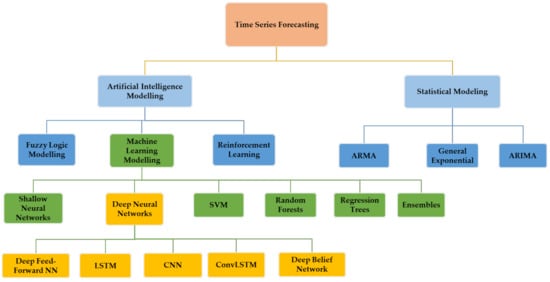
Figure 1.
Illustration of time series forecasting models.
2.2.1. Statistical-Based Methods
Recently, in the case of statistical-based load forecasting, the authors in [23] proposed Conditional Hidden Semi Markov Model (CHSMM) to forecast the residential appliance demand, which was evaluated using the Pecan Street database. The Auto-Regressive Moving Average (ARMA) model is considered as the famous traditional method for load forecasting. The authors in [24] applied the ARMA model to the California power market to make the electricity forecasting. In [25], an adaptive linear model (LM) procedure is employed to predict the residual component demand using the results of the Adaptive Circular Conditional Expectation (ACCE) process at each time window. Similarly, many more statistical methods are being improved to increase the accuracy of the forecast results. Statistical modelling is rarely utilized for the time series modelling of the energy load forecasting due to several limitations that affect the performance of the energy management system, such as high error probability; the reason is the input and output relation is represented by simple regression functions that are not effective to map the non-linear and dynamic uncertainty in the dataset.
2.2.2. Artificial Intelligence Methods
In [26], the fuzzy logic controller method is proposed for residential load forecasting using two inputs to draw the uncertain relation of the input and output. Furthermore, standard machine learning algorithms have been introduced to deal with the energy load forecasting problem such as random forest with decision trees, linear regression and gradient-boosted trees, which were evaluated on Spanish electricity load data with a ten-minute frequency [27]. In the problem of load forecasting, machine learning models as well as fuzzy logic-based models cannot accurately predict the trend of the load. There are always deviations in the case of forecasting the future consumption. This deviation is caused by the non-linearity and uncertainty in the consumption load data because it varies spatially and temporally. The spatial variation is due to the infrastructure and population of the domain. Even though using normalization to transform the data to the common scale, the temporal difference cannot be converged to the same scale [28]. To reduce a system’s computation burden and complete the real-time implementation, the deep neural network-based architectures came into existence to deal with the non-linear and dynamic system to improve the prediction performance.
In the field of energy load forecasting, which is formulated as a time series problem, many new ideas using deep learning have been successfully applied [29]. The reason behind this is the availability of a large amount of electricity data. Deep neural networks feed on data and the performance is directly proportional to dataset size. In the previous decade, several DNN architectures have been implemented to acquire a low error rate between the forecasted load and the actual consumption.

Table 1.
Review of the recent publications in energy load forecasting.
Table 1.
Review of the recent publications in energy load forecasting.
| Model | Author | Approach | Dataset Domain | Year | Dataset |
|---|---|---|---|---|---|
| Statistical Modelling | Yuting ji et al. [23] | Conditional Hidden Semi Markov Model | Household appliances | 2020 | Pecan street database |
| J. Nowicka-Zagrajek et al. [24], | ARMA | CAISO | 2002 | California, USA | |
| S.Sp. Pappas et al. [30] | ARMA | Hellenic Public Power Corporation S.A. | 2018 | Greece | |
| Nepal, B. et al. [31] | ARIMA | East Campus of Chubu University | 2019 | Japan | |
| Fatima Amara et al. [25] | ACCE with Linear Regression Model | Household electricity consumption | 2019 | Montreal, Quebec | |
| K.P. Amber et al. [32] | Multiple Regression Model | Administration building electricity consumption | 2015 | London, UK | |
| M. R. Braun et al. [33] | Multiple Regression Model | Supermarket electricity consumption | 2014 | Yorkshire, UK | |
| AI-Based Modelling | S.M. Mahfuz et al. [26] | Fuzzy Logic Controller | Residential apartment | 2020 | Memphis, TN, USA |
| Galicia et al. [27] | Ensembles | Spanish Peninsula | 2017 | Spanish electricity load data | |
| Grzegorz Dudek et al. [34] | LSTM and ETS | 35 European countries | 2020 | ENTSO-E | |
| Ljubisa Sehovac et al. [35] | S2S with Attention | Commercial building | 2020 | IESO, Ontario, Canada | |
| Yuntian Chen et al. [28] | Ensemble Long Short-Term Memory | Provincial (12 districts) | 2021 | Beijing, China | |
| T. Y. Kim et al. [36] | CNN-LSTM | Household electricity consumption | 2019 | UCI household electricity consumption dataset | |
| W. Kong et al. [37] | Sequence-to-Sequence | Household electricity consumption | 2019 | New South Wales, Australia | |
| D. Syed et al. [38] | LSTM | Household Electricity Consumption | 2021 | UCI household electricity consumption dataset | |
| Kunjin Chen et al. [39] | ResNet and Ensemble ResNet | North American Utility Dataset, ISO-NE, and GEFCom 2014 | 2018 | North American Utility Dataset, ISO-NE, and GEFCom 2014 | |
| Mohammad F. et al. [40] | Feed Forward Neural Network and Recurrent Neural Network | NYISO | 2019 | New York, USA |
3. Deep Learning Architectures for Energy Load Forecasting Modelling
3.1. LSTM-Based Architecture
LSTM is considered as one of the famous and most employed recurrent neural network (RNN) architectures for the time series modelling. The flow of information in the LSTM takes place in the recurrent fashion, which internally forms a chain-like structure, shown in Figure 2. RNN-based architectures have always performed well in the case of load forecasting. LSTM has the ability to memorize the long-term information using the memory cell state. The flow of information is controlled by four gates which are placed sequentially inside the LSTM cell, namely forget gate, input gate, output gate, and input node gate, as shown in Figure 3. Every time a new input comes, its information will be accumulated to the cell if the input gate is activated. The activation function is the main contributor in gate formation and has the ability to scale the input close to zero either (0, 1) or (−1, 0, 1). The previous cell status depends on the forget gate and can be forgotten in this process if the forget gate is ON, i.e., decision ranges from 0 to 1 where 0 means to forget this information and 1 means to keep it. The flow of the latest cell output to the final state is further controlled by the output gate .
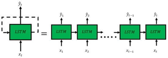
Figure 2.
Unrolled LSTM architecture.
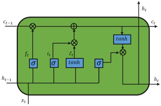
Figure 3.
Internal structure of LSTM cell.
Equations (1)–(6) represents mathematical formulation for the individual LSTM cell:
3.2. LSTM Encoder–Decoder-Based Architecture
In the load forecasting task, both the input and output are of variable-length sequence depending on the type of the problem [41]. To address these types of problems, encoder–decoder-based architecture came into existence. The model is comprised of two sub-models: the encoder, which takes in the input sequence, encodes it, and feeds it to next sub-model; and the decoder, which reads the encoded input sequence and makes a prediction to produce the output sequence, shown in Figure 4. In case of time series modelling, the LSTM model is mostly used in the decoder network, allowing it to both know what was predicted for the prior part in the sequence and accumulate internal state while outputting the sequence.
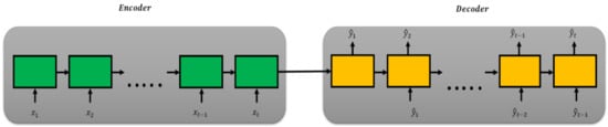
Figure 4.
Encoder–decoder for sequence-to-sequence learning for time series modelling.
3.3. CNN- and LSTM-Based Architecture
The CNN- and LSTM-based hybrid architecture is basically an encoder–decoder architecture, in which CNN acts as an encoder and LSTM acts as a decoder [36]. An encoder part with a one-dimensional CNN model has a convolutional layer that operates over a 1D sequence of the input data followed by a second convolutional layer. Each convolutional layer is followed by an activation layer and then a pooling layer whose job is to distill the output of the convolutional layer to the most salient elements. Both convolutional layers have ReLU activation function. The convolution layer applies the convolution operation to the incoming time series sequence and passes the results to the next layer. The pooling layer of the second convolutional layer is followed by a flatten layer to reduce the feature maps to a single one-dimensional vector. The flatten layer is connected to repeat vector layer to obtain the output from the previous layers and forward it to the decoder part of the network. The decoder part consists of the LSTM layer with a rectified linear unit (ReLU) activation function followed by a dropout of 50%. The LSTM output is fed to the dense fully connected layer called the time-distributed layer, followed by one more fully connected layer that interprets the output of the model.
3.4. ConvLSTM Architecture
ConvLSTM is used to capture spatial–temporal dependency in the time-series electricity consumption dataset. ConvLSTM is said to be an extension of the CNN-LSTM approach described previously. ConvLSTM performs the convolutions as in CNN as part of the LSTM for each time step. Recently, with this configuration, it boomed image recognition and prediction with excellent results [17,42,43]. ConvLSTM uses convolutions directly as part of the reading input into the LSTM cells themselves, as shown in Figure 5. Recently, [44] has employed a ConvLSTM-based load forecasting model to produce least error with high accuracy on the time series data collected in Maine, USA. This model has a CNN-based encoder which extracts the features from the time series data and ConvLSTM further processes the spatiotemporal information.
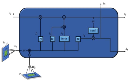
Figure 5.
The internal structure of ConvLSTM cell.
ConvLSTM has been applied to various tasks such as predicting tumor growth [45], biological age estimation [42], spatial feature extraction for hyperspectral image (HSI) classification [43], etc. Depending on the applications, ConvLSTMs have similar variants such as ConvLSTM 1D, ConvLSTM 2D, and ConvLSTM 3D with a difference in the type of the filter used to initiate the operations.
The mathematical formulation of the ConvLSTM cell can be expressed as:
where denotes the input of the current cell; and are the state and output of the last cell, respectively. ‘∗’ asterisk means the convolution operation. W denotes the convolution filter, which is a 2-D convolution filter with a k × k kernel. Specially, the definitions of , , , , and are similar to that of LSTM architecture; however, the data dimensions and processing methods are different. This special structure enables ConvLSTM to extract a more effective feature representation than CNN. Furthermore, compared with LSTM, the implementations of three gate mechanisms are extended from one-dimensional to multi-dimensional convolution operation.
4. The Proposed Energy Load Forecasting System
The whole structure of the proposed framework in this paper is described in Figure 6. For a deeper understanding of the proposed model, a more detailed description is given below:
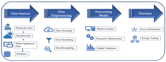
Figure 6.
Framework of the proposed energy load forecasting system.
4.1. Data Sources
To build an energy management system, intelligent integration of various distributed energy resources (DERs), end devices, and automatic control operations are needed. In the IoT era, end devices are connected to the centralized or distributed system which collects the data, generated periodically by the end devices, using the advanced sensor technology, and then the response signal is sent to the counterpart actuators to carry out the decided actions from the energy management system.
Based on the scale of the deployment of the energy management system from where we need to collect data, it is categorized as:
- Smart Home Energy Management System (SHEMS):
In a smart building/home, we access the data from the different entities in the household (appliances energy consumption, aggregated) and add it to a large database file [19]. The daily electricity consumption data are collected from an individual household meter or an aggregator for an adequate time period using sensors from the so-called Advanced Metering Infrastructure (AMI).
The AMI consists of three major elements: electricity meters, a bidirectional communication channel, and a data storage which collects the time series electricity data periodically. AMI enables the SHEMS to provide a number of vital functions such as measuring electricity consumption, security, and communication with the end devices and the utilities [46].
- Smart Grid Energy Management System (SGEMS):
The transition from the conventional and unidirectional power grid to smart power grids has made the opportunities available to deal with the demand and supply curve intelligently. With IoT assistance, the energy management in smart power grids is able to reach every corner of a city or a local area to collect the data and the behavior of the grid entities [1,2], which paved the way to utilize that data to improve the system at a higher level (city/microgrid).
4.2. Data Preprocessing
After the data acquisition, the raw data needs to be preprocessed before being fed to the machine to make the prediction. This step is necessary because the raw data have a lot of noisy datapoints and missing data. The data cleaning step is taken to adjust the numerical differences among the data points using min–max normalization so that all the attributes of the dataset lie on the same scale, as shown in Figure 7. The normalization technique helps to improve the performance of the model training process due to the significant differences among target data; this helps to increase the speed of the training process [47]. The min–max normalization is formulated as presented in Equation (13):
where x is an original value, is the maximum value of x, is the minimum value of x, and z is the normalized value. Raw data are to be processed and furnished according to the model prerequisites. All deep learning-based models feed on the data; more data leads to healthier training. However, on the other hand, only clean data can make it possible to improve the model performance at its best. It is the nature of the data that decides the job of the designed model.
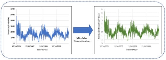
Figure 7.
Normalizing the actual electricity consumption data using min–max normalization.
Furthermore, we resample the whole dataset to change the entries from minute-based to daily-based using sklearn library. As with the LSTMs for univariate data in a prior section, the prepared samples must first be reshaped. The LSTM expects data to have a three-dimensional structure of [samples, timesteps, features] and the same for the CNN-based architecture, while in the case of ConvLSTM it is [samples, timesteps, rows, cols, channels], and in this case, we only have one feature, so the reshape is straightforward. In this work, the data we are working with is having lower granularity (downsample from the higher frequency to lower frequency). The granularity of original raw data usually have a minutely consumption pattern. By using the resampling technique, the whole dataset goes through resampling process to obtain hourly or daily consumption data.
4.3. Forecasting Model
Multiple deep learning architectures explained in the previous section are put under investigation to select the best one in terms of both generalization capability and reduced error. The proposed energy load forecasting model is based on encoder–decoder architecture having ConvLSTM as an encoding network and LSTM employed as a decoding network. Before going for the selection of the final DNN architecture, different model hyperparameters such as activation function, batch size, dropout, learning rate, number of neurons in each hidden layer, optimization algorithm, training epochs, etc. are to be optimized. The most common loss function called the mean absolute error is used to draw the training and validation curves. In the proposed deep learning model, Adam optimizer is utilized as an optimization algorithm after investigating it against RMSProp. Overfitting of the proposed model during training is addressed by using dropout regularization and further L2 regularization is added after each LSTM layer which adds a penalty term to the loss function of the network for large weights. Regularization results in model simplicity to learn only the relevant patterns in the training data.
4.4. Decision
In the energy market, intelligent decisions which are taken by the EMS with the help of making the accurate and precise forecasting of the energy consumption can lead to a sustainable smart grid. The ability to provide decisions in real time is directly proportional to the reliability in smart grids and thereby increasing end user’s confidence in the smart grid technology. Peer-to-peer energy trading can provide a way for energy marketing by virtue of which prosumers can make a profit by trading their surplus of energy gathered from renewable resources (e.g., PVs) during the peak hours and stored energy in storage devices such as energy storage systems (ESS) during the non-peak hours [6]. Customers can save on their energy bills by buying cheap energy from their peers or making the use of clean renewable energy instead of buying directly from the grid, thereby decreasing the load on the grid. To stabilize the grid power, the customers can participate in the energy markets by selling the extra energy back to the grid during peak hours, which can shave off the instantaneous peaks and also results in the money-making of the customers.
5. Proposed Deep Learning Architecture for Energy Load Forecasting
This work proposes a novel energy load forecasting model based on the sequence-to-sequence encoder–decoder architecture, that deploys deep convolutional long short-term memory network architecture, also called ConvLSTM. A conventional encoding-decoding structure is not enough to deal with the spatiotemporal data. To deal with spatio-temporal data, there is a need for special network architecture that can work in both domains to capture spatial as well as temporal characteristics. ConvLSTM is a kind of recurrent layer, just like the LSTM, but internal matrix multiplications are exchanged with convolution operations, while in case of LSTMs, it is a Hadamard product. Convolution is used for both input-to-state and state-to-state connection making the final state have a large receptive field. The proposed deep learning model is based on the encoder–decoder architecture, which consists of ConvLSTM2D-based encoder and a decoder consists of LSTM layers. Furthermore, to the best of our knowledge, this work has simultaneously considered two hyperparameters to build a more generalized model.
5.1. ConvLSTM-LSTM Architecture for Energy Load Forecasting
The proposed ConvLSTM-LSTM is an encoder–decoder network architecture in which the ConvLSTM forms the encoding part and the LSTM forms the forecasting or decoding part of the whole architecture, as shown in Figure 8. In convolutional long short-term memory, each time step of data is defined as an image of rows and columns data points. The ConvLSTM (we used interchangeably ConvLSTM2D) model was first introduced to deal with precipitation nowcasting [17] due to its capacity of extracting spatiotemporal information. Equations (7)–(12) define the operations in the ConvLSTM network. In the proposed deep learning architecture, we stacked multiple ConvLSTM layers to form an encoder network which takes the input data and performs convolutions on it and passes its output to the flatten layer. The flatten layer reshapes it into the one-dimensional output and is followed by a repeat vector layer. The repeat vector layer repeats the incoming inputs a specific number of times, the same as the original input, which can be fed to the decoding network. Hyperparameters in the ConvLSTM layer are similar to that of CNN. After conducting the many trial experiments, we finally settled down to select and finalize the hyperparameters including the number of filters, kernel size, activation function, and input shape for the ConvLSTM layers. Similarly, it is hard to decide the number of hidden layers of ConvLSTM to build the encoding network without training it with different combinations. After conducting series of experiments, we settle with four ConvLSTM stacked layers to design encoder network.
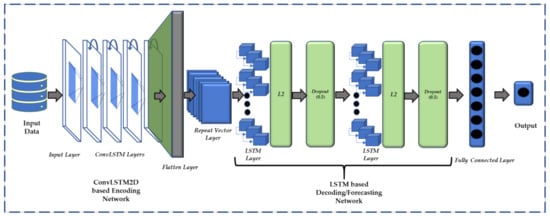
Figure 8.
ConvLSTM-LSTM-based encoder–decoder architecture for energy load forecasting.
The decoding network consists of LSTM layers. LSTM as a special RNN structure has proven successful and is widely used for modeling long-range dependencies in various previous studies [11,12,17,23]. The contribution of LSTM is recurrent connections, memory cell , and the self-parameterized and controlling gates, which essentially controls the flow of the state information. During the training of LSTM, one advantage of using the memory cell and gates is to prevent vanishing gradients, which is a critical problem existing in simple RNN-based models. Each LSTM layer is followed by a dropout layer which reduces the overfitting of the network on the training dataset. Furthermore, L2 regularization is applied to both LSTM layers to reduce the complexity of the model. It does so by adding a penalty term to the loss function. Following it, two consecutive time-distributed fully connected layers produce the output of the whole network, i.e., forecasting result. Table 2 shows the architecture of the proposed energy load forecasting model.
Table 2.
Architecture of the proposed energy load forecasting model.
5.2. Implementation Details
Deep neural networks are stochastic machine learning algorithms. In our case, we implemented a novel encoder–decoder network architecture for time series data to forecast energy consumption. The random initial weight matrix allows the model to train from a different starting point in the search space. In a neural network, the weights and biases of the hidden layers are updated on the basis of the result of the loss function signal. The training algorithm decides the magnitude of the weights in the weight matrix which causes the network to output the expected values, given some input data. Each layer is characterized by its weight matrix, bias, and activation function. The hidden layers in the encoder take the input matrix of electricity data and apply the filters on it using the convolutional operations to obtain the feature maps, which is also a kind of modified matrix of size depending on the size and the number of the filters used in that layer. In case of encoder–decoder architecture, the format of output produced by the encoder needs to be same as the input data so as to feed it to the decoder network; for that, it is traverses through flatten layer to reach to the decoder. This is the forward movement of information known as the forward propagation. After, calculating the loss using the loss function, the error signal is sent back to the preceding layers and fine tuning the weights is made to ensure lower error rates, so as to increase generalization. This process is known as back-propagation. Once all the data have gone through forward–backward propagation, the final weight and bias matrices are formed to make predictions/forecasting.
In this study, we formulated energy load forecasting as a multi-step time series forecasting problem, which is an autoregressive problem. That means the next timestep prediction is the function of observations at previous timesteps. We developed a model with an encoding network consisting of multiple ConvLSTM layers and the decoding network with multiple layers of LSTM layer with 200 units. Each LSTM layer has the activation function ReLU. To speed up the training, we employed two regularization methods: dropout and L2 regularization. Dropout had a value of 0.5, which means that 50% of the hidden neurons are left untrained to reduce the complexity of the model. Furthermore, L2 regularization, also called Ridge Regression, adds the squared magnitude of the coefficient as a penalty term to the loss function. The value of L2 regularization is set to 0.001. The encoder network is followed by a time-distributed fully connected layer with 100 nodes that will take the features learned by the LSTM layers. Finally, an output layer directly predicts a vector with seven elements, one for each day in the output sequence.
The training loss is measured using a mean squared error as a loss function because it is proven as a good error metric for validation loss. We use the efficient Adam optimizer as an implementation of stochastic gradient descent and train the model for 100 epochs with multiple batch sizes. Finally, after continuous experimentation, the batch size of 256 is used to train the network. A smaller batch takes a long time to train but provides favorably good prediction results while, as in our case, the larger batch size gives the better results. This means that results may vary when the model is evaluated. To evaluate the performance of the different models, we train the proposed model multiple times and calculate an average of model performance.
We have a one-dimensional sequence of total energy consumption data, which can be interpreted as two subsequences with a length of seven days each. To make the day ahead forecast using the previous weeks data, this requires that a proposed model forecasts the total active power for each day over the next seven days. This could be helpful for the aggregator in planning the demand and supply for the household for a specific period. The ConvLSTM can then read across the two time-steps and follow the basic CNN process on the seven days of data. The ConvLSTM layer output is a combination of a Convolution and an LSTM output. Just like the LSTM, it returns a sequence as a 5D tensor with shape (samples, time steps, rows, columns, channels).
5.3. Backtesting/Validating Proposed Deep Learning Model for Energy Load Forecasting
Validating the deep learning model is the fundamental step to check the performance of the proposed model on the unseen data with a similar distribution as of the training data. Before evaluating a model for time series forecasting, the training dataset is split in such a way that some is used to train the model, and some is kept back, called validation data or development data. When the model is trained on the training data, parallelly it makes the predictions on the validation data for that period. The prediction results on the validation data will provide a good proxy for how the model will perform when we use it operationally.
In the proposed model, we use the walk forward validation method to validate the model, which is similar to the k-fold cross validation [48,49]. This method makes the forecast at each time step by utilizing the sliding window mechanism, which depends on the number of the samples or observations in a window. After selecting the window size, the training starts and makes a step ahead prediction. This predicted value is stored in the window by expanding its size, and the above process is repeated, as shown in Figure 9.
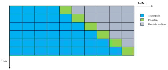
Figure 9.
Graphical representation of walk-forward validation—backtesting.
In fact, by doing the multiple split across the different time periods, the training data expanding each fold makes it robust in choosing the model parameters. On the other hand, the step-by-step estimation increases the computational cost, but this is not expensive if the dataset is small. In our case, after resampling the data from minutes to days or hours, the dataset size reduction was manifold, which makes the walk forward validation method a promising way to deal with the issue of the reduced dataset. Furthermore, it decreases the chance for the model to become overfitted on the training data.
5.4. Evaluation Metrics
The performance of the proposed model is evaluated and compared using three metrics. The first metric is the mean absolute percentage error (MAPE), the second metric is the mean squared error (MSE), and the third metric is the root mean square error (RMSE), which are mathematically represented as follows:
In the above equations, is the real value, is the predicted value, and is the total number of samples.
6. Experimental Results and Discussion
In this section, we compare the performance of the proposed energy load forecasting model with the state-of-the-art deep learning models. Two different datasets are considered under analysis, namely household electricity consumption dataset available online in the Machine Learning Repository of the University of California, Irvine and New York Independent System Operator dataset to verify the qualitative as well as quantitative performance of the proposed model.
6.1. Data Description
6.1.1. UCI Individual Household Dataset
The dataset is available in the dataset archive of the University of California, Irvine (UCI) Machine Learning repository [50]. The dataset contains 2,075,259 data points having nine attributes. The dataset ranges over a period of 4 years, with an entry of minutely electricity consumption, from 12 December 2006 to 26 November 2010. The household power consumption dataset describes electricity usage for a single household. The different attributes in the energy consumption data are described in Table 3. The main goal of the proposed model is that it can be helpful within the household in planning energy expenditures and take a proper decision to trade the energy in the community microgrid which is not in the scope of this paper. It is used for planning electricity supply–demand for a specific household. In this work, framing of the dataset is performed to downsample the per-minute frequency of power consumption to total daily consumptions, which yields 1443 data samples of the aggregated load on the daily basis. For training purpose univariately energy consumption is selected. Up-sampling or down-sampling the dataset depends on what target we are interested in forecasting. The resample () function available in the Pandas library by passing the argument ‘D’ which allows the loaded data indexed by date–time to be grouped by day. We can then calculate the sum of all observations for each day and create a new dataset of daily power consumption data for each of the eight variables.
Table 3.
The features of individual household power consumption dataset.
6.1.2. New York Independent System Operator (NYISO) Dataset
The energy load data are collected from New York Independent System Operator (NYISO). The dataset contains the daily records with hourly entries of electricity data for the whole New York state, consisting of 11 different regions [51]. The load data in raw form consists of 12 columns with the first column containing timestamp and the next remaining columns represent the electricity consumption for the regions in the New York state. Pre-processing clean data are obtained, which are then used to train the deep learning models. The dataset ranges from May 2007 to May 2014. The training dataset consists of hourly data in the form of a table having 53,321 datapoints with 10 different features. To train our model, we need to reshape it according to the input dimension of the model. Downsampling the dataset, we obtain the total of 2577 data point, shown in Figure 10. The validation dataset consists of 30% of the test dataset. In this case study, city-wide energy consumption data are selected to prove the scalability and computational competency of the proposed model.
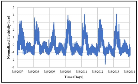
Figure 10.
Normalized daily electricity load in NYISO dataset.
6.2. Parameter Selection for Training the Proposed Energy Load Forecasting Model
To train a deep neural network, different parameters and hyperparameters such as the batch size of the training set, number of hidden layers, activation function in the hidden layers, dropout, optimization algorithm number of training epochs, etc. are analyzed to select the best architecture for the energy load forecasting task. The number of epochs to train is selected as 100 to avoid over training of the network, which increases the computational time without improving the accuracy of the prediction. In the case of hidden layers, the ReLU activation function is opted for as compared to hyperbolic tangent (tanh) as the number of hidden layers grows up to avoid vanishing gradient. Furthermore, two regularization parameters, namely dropout and L2 regularization, are used to avoid overfitting of the model and to improve the generalization. The batch size is kept at 256 after training with 64, 128, and 512 as well to decrease the training loss and the mean square error (MSE) is used as a loss function. Table 4 provides the list of hyperparameters selected for the proposed energy load forecasting model.
Table 4.
Hyperparameter setting for the proposed model.
In addition, different optimizers have been employed such as RMSProp [52] and Adam [53]. Based on the empirical results, we have selected Adam optimizer for this work. Adam is said to have properties of both Adadelta and RMSProp and hence performs comparatively better for most of the problems. In [53], there are some simulations where Adam is compared to SGDNesterov, AdaGrad, RMSProp (MNIST, IMDB, CIFAR10). Adam performs very well compared to the others. The authors find that Adam converges faster than AdaGrad in a convolutional network. To testify the above statement, we simulated different deep learning architectures using Adam and RMSProp optimizers to draw the training and validation curves, which provide some intuition of selecting the optimizer well suited for our task to achieve better generalization. In Figure 11, the results of training and validation curves of simulated DNN architectures are shown when trained with Adam and RMSProp optimizers on the UCI dataset as well as on the NYISO dataset. After analyzing the reported figures, we deduced that the optimal optimizer to be used for time series forecasting is Adam. This algorithm is easy to implement, computationally efficient, converges to attain generalization, and has fewer memory requirements.
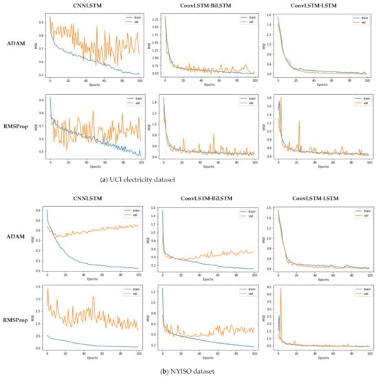
Figure 11.
Illustration of training loss and validation loss using different optimizers for both datasets, (a) UCI electricity dataset, and (b) NYISO dataset.
6.3. Performance with UCI Individual Household Dataset
In this section, we evaluate the proposed energy load forecasting model against the various encoder–decoder-based deep learning architecture quantitatively as well as qualitatively to obtain the least error in forecasting the total daily energy consumption of a single household. It becomes clear that the proposed energy load forecasting model comparatively out-performs the existing state-of-the-art load forecasting models, as shown in Table 5. Each model analyzed in this work has specific built-in characteristics which make them feasible candidates for performing energy load forecasting task.
Table 5.
Comparison of the evaluation metrics on the univariate UCI household electricity dataset.
In the case of UCI dataset, after forecasting the aggregated daily energy consumption for a weekly basis, the proposed model achieves high performance in terms of having the least errors. The proposed architecture achieves 9.4%, 12%, and 3.9% more least error rate in terms of RMSE, MSE, and MAPE, respectively, than the CNNLSTM-based model proposed in [32], which is the combination of two Conv1D layers followed by a single LSTM layer. Similarly, we achieve better performance than LSTM-LSTM encoder–decoder architecture by the improvement of 6.6%, 1.5%, and 7.9% in the case of RMSE, MSE, and MAPE, respectively. In the case of above two models, achieving higher performance is possible at the cost of computational time. The ConvLSTM-BiLSTM model consists of an encoder having a single ConvLSTM layer and decoder with one LSTM layer. The proposed architecture achieves a lower error rate than ConvLSTM-BiLSTM in the case of evaluation metrics and with less computational time and a lower number of parameters used. The ConvLSTM-LSTM performs 6.9%, 7.2%, and 9.1% better than ConvLSTM-BiLSTM in the case of RMSE, MSE, and MAPE, respectively.
In Figure 12, qualitative results depict that when three models—CNNLSTM, Con-vLSTM-BiLSTM, and ConvLSTM-LSTM—are tested on the test set of 46 sample weeks for different days, each one tries to follow the dynamic trend of the energy consumption for each day. The blue curve represents the actual energy consumption and the orange curve represents the prediction result using the various deep learning models. The figure con-sists of only three alternative days of a week to show the robustness of the models. Each day of a week has a different consumption pattern with dynamically changing. Observing Figure 13, it provides the average values of the evaluation metrics considering one week starting from Sunday and ends at Saturday, which also gives the intuition of using ConvLSTM-LSTM-based energy load forecasting model compared to other architectures.
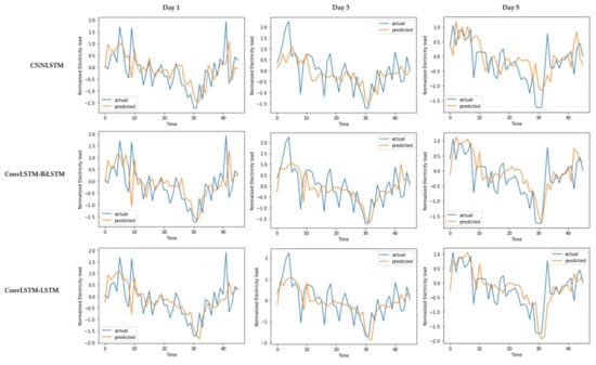
Figure 12.
Daily total actual consumption vs. prediction results over a test samples for different days in a week with UCI household electricity dataset.
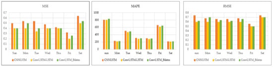
Figure 13.
Evaluation metrics for different days in a week with UCI electricity dataset.
6.4. Performance with New York Independent System Operator (NYISO) Dataset
In the case of the NYISO dataset, after preprocessing the dataset to make it compatible with the model for training purpose, univariate data consisting of total load consumption values is selected as the input to the model. Forecasting the aggregated daily energy consumption over one week, the proposed model achieves better performance in terms of achieving the least forecasting error. By observing Table 6, the proposed architecture in forecasting the total consumption achieves better performance with 3.8%, 24.1%, and 18.8% amounts of decrease in the error rate in terms of RMSE, MSE, and MAPE, respectively, compared to CNNLSTM-based model. In the case of LSTM-based encoder–decoder, the proposed model continues to outperform by the decrease of 5.5%, 19.5%, and 20.45% in terms of RMSE, MSE, and MAPE, respectively. Similarly, comparing to the ConvLSTM-BiLSTM model, which consists of an encoder, the proposed architecture achieves lower error than in terms of evaluation metrics and with less computational time and number of parameters used as in the case of the previous dataset. The ConvLSTM-LSTM performs 1.1%, 10.46%, and 11.17% better than ConvLSTM-BiLSTM when compared in terms of RMSE, MSE, and MAPE, respectively. We simulated the proposed model against the existing models on alternative days of the week considering the whole test dataset to check the scalability and robustness. The results of experimentation in Figure 14 clearly show that the trend learning ability of the proposed energy load forecasting model is comparable to the existing architectures. Similarly, in Figure 15, average values of the evaluation metrics RMSE, MSE, and MAPE have been illustrated to show the superiority of the proposed model in only RMSE and MAPE, while ConvLSTM-BiLSTM has the upper hand in the case of the averaged MSE value.
Table 6.
Comparison of the evaluation metrics on the univariate NYISO electricity dataset.
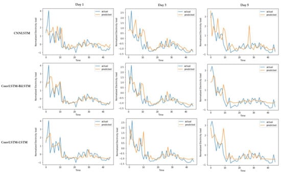
Figure 14.
Daily total actual consumption vs. prediction results over a test samples for different days in a week with NYISO dataset.
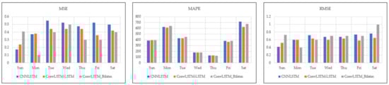
Figure 15.
Evaluation metrics for different days in a week with NYISO electricity dataset.
We used Keras (https://keras.io/) library with TensorFlow (https://www.tensorflow.org/) in the backend to build the deep learning models. All experiments were performed using an NVIDIA GeForce GTX 970 running on a Microsoft Windows 10 (operating system) machine with an Intel Core-i7 processor and 8 GB RAM.
7. Conclusions
This paper proposed a novel ConvLSTM-LSTM encoder–decoder-based load forecasting model for challenging task of individual residential load forecasting on a daily basis for over a week. The proposed model consists of multiple ConvLSTM layers which encode the input and LSTM-based decoder to deal with the uncertainty, long-range dependency, and dynamic characteristics of spatio-temporal electricity load data. ConvLSTM proved its ability to recognize the energy consumption pattern to produce the activation map consisting of the salient features of input data which were later fed to the LSTM layers to output prediction results. The proposed ConvLSTM-LSTM-based load forecasting model was comprehensively tested and compared with the multiple benchmark DNN architectures on a real-world dataset, i.e., UCI individual household dataset and NYISO dataset. The results proved that the proposed model qualitatively as well as quantitatively outperformed the existing DNN architectures by reducing the error by a good percentage.
Since this work was limited to the univariate input dataset for training the DNN architectures, future work will focus on including some more influencing factors which are highly correlated with the energy consumption of a particular household or a power grid, such as weather data (temperature), household occupancy, lagged load, etc. Data analytics has made an option available, i.e., data-centric artificial intelligence which focuses on furnishing the data rather than modifying the model parameters. One more way to further research is to consider other variants of the ConvLSTM such as bidirectional ConvLSTM, ConvLSTM 3D, etc. Furthermore, there is the potential of implementing edge computing (EC) in smart grids to reduce the computing constraints performed by ICT in smart grids, which can speed up the power grid operations such as controlling, dispatching, scheduling, and energy trading.
Author Contributions
Conceptualization, F.M. and Y.-C.K.; methodology, F.M.; software, F.M.; validation, F.M., M.A.A., and Y.-C.K.; writing—original draft preparation, F.M. and M.A.A.; writing—review and editing, F.M., M.A.A. and Y.-C.K. All authors have read and agreed to the published version of the manuscript.
Funding
This work was supported by the National Research Foundation of Korea (NSF) grant funded by the Korean Government (2021R1I1A305872911).
Institutional Review Board Statement
Not applicable.
Informed Consent Statement
Not applicable.
Data Availability Statement
Not applicable.
Conflicts of Interest
The authors declare no conflict of interest.
References
- Feng, C.; Wang, Y.; Chen, Q.; Ding, Y.; Strbac, G.; Kang, C. Smart grid encounters edge computing: Opportunities and applications. Adv. Appl. Energy 2021, 1, 100006. [Google Scholar] [CrossRef]
- Gavriluta, C. Smart Grids Overview—Scope, Goals, Challenges, Tasks and Guiding Principles. In Proceedings of the 2016 IEEE International Forum on Smart Grids for Smart Cities, Paris, France, Day 16–18 October 2016. [Google Scholar]
- Alotaibi, I.; Abido, M.A.; Khalid, M.; Savkin, A.V. A Comprehensive Review of Recent Advances in Smart Grids: A Sustainable Future with Renewable Energy Resources. Energies 2020, 13, 6269. [Google Scholar] [CrossRef]
- IEEE Smart Grid Big Data Analytics; Mchine Learning; Artificial Intelligence in the Smart Grud Working Group. Big Data Analytics in the Smart Grid. IEEE Smart Grid. 2017. Available online: https://smartgrid.ieee.org/images/files/pdf/big_data_analytics_white_paper.pdf (accessed on 27 September 2021).
- Weir, R.; Providing Non-Stop Power for Critical Electrical Loads. The Hartford Steam Boiler Inspection and Insurance Company. Available online: https://www.hsb.com/TheLocomotive/ProvidingNon-StopPowerforCriticalElectricalLoads.aspx (accessed on 29 June 2021).
- IRENA. Innovation landscape Brief: Peer-To-Peer Electricity Trading; International Renewable Energy Agency: Abu Dhabi, United Arab Emirates, 2020. [Google Scholar]
- He, K.; Zhang, X.; Ren, S.; Sun, J. Deep Residual Learning for Image Recognition. arXiv 2016, 770–778. [Google Scholar] [CrossRef] [Green Version]
- Cho, K.; van Merriënboer, B.; Gulcehre, C.; Bougares, F.; Schwenk, H.; Bengio, Y. Learning Phrase Representations using RNN Encoder–Decoder for Statistical Machine Translation. In Proceedings of the 2014 Conference on Empirical Methods in Natural Language Processing (EMNLP), Doha, Qatar, 26–28 October 2014. [Google Scholar]
- Siraj, A.; Chantsalnyam, T.; Tayara, H.; Chong, K.T. RecSNO: Prediction of Protein S-Nitrosylation Sites Using a Recurrent Neural Network. IEEE Access 2021, 9, 6674–6682. [Google Scholar] [CrossRef]
- Alam, W.; Tayara, H.; Chong, K.T. XG-ac4C: Identification of N4-acetylcytidine (ac4C) in mRNA using eXtreme gradient boosting with electron-ion interaction pseudopotentials. Sci. Rep. 2020, 10, 20942. [Google Scholar] [CrossRef] [PubMed]
- Abdelbaky, I.; Tayara, H.; Chong, K.T. Prediction of kinase inhibitors binding modes with machine learning and reduced descriptor sets. Sci. Rep. 2021, 11, 706. [Google Scholar] [CrossRef]
- Mnih, V.; Kavukcuoglu, K.; Silver, D.; Veness, J.; Bellemare, M.G.; Graves, A.; Riedmiller, M.; Fidjeland, A.K.; Ostrovski, G.; Petersen, S.; et al. Human-level control through deep reinforcement learning. Nature 2015, 7540, 518–529. [Google Scholar] [CrossRef]
- Hochreiter, S.; Schmidhuber, J. Long Short-term Memory. Neural Comput. 1997, 9, 1735–1780. [Google Scholar] [CrossRef]
- Bai, M.; Goecke, R. Investigating LSTM for Micro-Expression Recognition. In Proceedings of the Companion Publication of the 2020 International Conference on Multimodal Interaction, Utrecht, The Netherlands, 25–29 October 2020; Association for Computing Machinery (ACM): Utrecht, The Netherlands, 2020; pp. 7–11. [Google Scholar]
- Mohd, M.; Qamar, F.; Al-Sheikh, I.; Salah, R. Quranic Optical Text Recognition Using Deep Learning Models. IEEE Access 2021, 9, 38318–38330. [Google Scholar] [CrossRef]
- Shaoxiang, C.; Yao, T.; Jiang, Y.-G. Deep Learning for Video Captioning: A Review. In Proceedings of the Twenty-Eighth International Joint Conference on Artificial Intelligence (IJCAI-19), Macao, China, 10–16 August 2019. [Google Scholar]
- Shi, X.; Zhourong, C.; Wang, H.; Yeung, D.-Y.; Wong, W.-K.; Woo, W.-C. Convolutional LSTM Network: A Machine Learning Approach for Precipitation Nowcasting. In NIPS; NeurIPS: Montreal, QC, Canada, 2015. [Google Scholar]
- Aman, S.; Simmhan, Y.; Prasanna, V.K. Energy management systems: State of the art and emerging trends. IEEE Commun. Mag. 2013, 51, 114–119. [Google Scholar] [CrossRef]
- Hussain, S.; El-Bayeh, C.Z.; Lai, C.; Eicker, U. Multi-Level Energy Management Systems Toward a Smarter Grid: A Review. IEEE Access 2021, 9, 71994–72016. [Google Scholar] [CrossRef]
- Liu, Y.; Yang, C.; Jiang, L.; Xie, S.; Zhang, Y. Intelligent Edge Computing for IoT-Based Energy Management in Smart Cities. IEEE Netw. 2019, 33, 111–117. [Google Scholar] [CrossRef]
- Mohan, N.; Soman, K.; Kumar, S.S. A data-driven strategy for short-term electric load forecasting using dynamic mode decomposition model. Appl. Energy 2018, 232, 229–244. [Google Scholar] [CrossRef]
- Syed, D.; Abu-Rub, H.; Ghrayeb, A.; Refaat, S.S. Household-Level Energy Forecasting in Smart Buildings Using a Novel Hybrid Deep Learning Model. IEEE Access 2021, 9, 33498–33511. [Google Scholar] [CrossRef]
- Ji, Y.; Buechler, E.; Rajagopal, R. Data-Driven Load Modeling and Forecasting of Residential Appliances. IEEE Trans. Smart Grid 2020, 11, 2652–2661. [Google Scholar] [CrossRef] [Green Version]
- Nowicka-Zagrajeka, J.; Weronb, R. Modeling electricityloads in California: ARMA models with hyperbolic noise. Signal Process. 2002, 82, 1903–1915. [Google Scholar] [CrossRef] [Green Version]
- Amara, F.; Agbossou, K.; Dubé, Y.; Kelouwani, S.; Cardenas, A.; Hosseini, S.S. A residual load modeling approach for household short-term load forecasting application. Energy Build. 2019, 187, 132–143. [Google Scholar] [CrossRef]
- Alam, S.M.M.; Ali, M.H. Equation Based New Methods for Residential Load Forecasting. Energies 2020, 13, 6378. [Google Scholar] [CrossRef]
- Galicia, A.; Torres, J.; Martínez-Álvarez, F.; Troncoso, A. A novel spark-based multi-step forecasting algorithm for big data time series. Inf. Sci. 2018, 467, 800–818. [Google Scholar] [CrossRef]
- Chen, Y.; Zhang, D. Theory-guided deep-learning for electrical load forecasting (TgDLF) via ensemble long short-term memory. Adv. Appl. Energy 2021, 1, 100004. [Google Scholar] [CrossRef]
- Gamboa, J. Deep Learning for Time-Series Analysis, in Seminar on Collaborative Intelligence. arXiv 2017, arXiv:1701.01887. [Google Scholar]
- Pappas, S.; Ekonomou, L.; Karampelas, P.; Karamousantas, D.; Katsikas, S.; Chatzarakis, G.; Skafidas, P. Electricity demand load forecasting of the Hellenic power system using an ARMA model. Electr. Power Syst. Res. 2010, 80, 256–264. [Google Scholar] [CrossRef]
- Nepal, B.; Yamaha, M.; Yokoe, A.; Yamaji, T. Electricity load forecasting using clustering and ARIMA model for energy management in buildings. Jpn. Arch. Rev. 2019, 3, 62–76. [Google Scholar] [CrossRef] [Green Version]
- Amber, K.P.; Aslam, M.W.; Mahmood, A.; Kousar, A.; Younis, M.Y.; Akbar, B.; Chaudhary, G.Q.; Hussain, S.K. Energy Consumption Forecasting for University Sector Buildings. Energies 2017, 10, 1579. [Google Scholar] [CrossRef] [Green Version]
- Braun, M.; Altan, H.; Beck, S. Using regression analysis to predict the future energy consumption of a supermarket in the UK. Appl. Energy 2014, 130, 305–313. [Google Scholar] [CrossRef] [Green Version]
- Dudek, G.; Pelka, P.; Smyl, S. A Hybrid Residual Dilated LSTM and Exponential Smoothing Model for Midterm Electric Load Forecasting. IEEE Trans. Neural Netw. Learn. Syst. 2021, PP, 1–13. [Google Scholar] [CrossRef] [PubMed]
- Sehovac, L.; Grolinger, K. Deep Learning for Load Forecasting: Sequence to Sequence Recurrent Neural Networks with At-tention. IEEE Access 2020, 8, 36411–36426. [Google Scholar] [CrossRef]
- Kim, T.-Y.; Cho, S.-B. Predicting residential energy consumption using CNN-LSTM neural networks. Energy 2019, 182, 72–81. [Google Scholar] [CrossRef]
- Kong, W.; Dong, Z.Y.; Jia, Y.; Hill, D.J.; Xu, Y.; Zhang, Y. Short-Term Residential Load Forecasting Based on LSTM Recurrent Neural Network. IEEE Trans. Smart Grid 2019, 10, 841–851. [Google Scholar] [CrossRef]
- Syed, D.; Abu-Rub, H.; Ghrayeb, A.; Refaat, S.S.; Houchati, M.; Bouhali, O.; Banales, S. Deep Learning-Based Short-Term Load Forecasting Approach in Smart Grid with Clustering and Consumption Pattern Recognition. IEEE Access 2021, 9, 54992–55008. [Google Scholar] [CrossRef]
- Chen, K.; Chen, K.; Wang, Q.; He, Z.; Hu, J.; He, J. Short-Term Load Forecasting with Deep Residual Networks. IEEE Trans. Smart Grid 2018, 10, 3943–3952. [Google Scholar] [CrossRef] [Green Version]
- Mohammad, F.; Kim, Y.-C. Energy load forecasting model based on deep neural networks for smart grids. Int. J. Syst. Assur. Eng. Manag. 2019, 11, 824–834. [Google Scholar] [CrossRef]
- Marino, D.L.; Amarasinghe, K.; Manic, M. Building energy load forecasting using Deep Neural Networks. In Proceedings of the IECON 2016—42nd Annual Conference of the IEEE Industrial Electronics Society, Florence, Italy, 23–26 October 2016; pp. 7046–7051. [Google Scholar]
- Rahman, S.A.; Adjeroh, D.A. Deep Learning using Convolutional LSTM estimates Biological Age from Physical Activity. Sci. Rep. 2019, 9, 11425. [Google Scholar] [CrossRef] [PubMed] [Green Version]
- Hu, W.-S.; Li, H.-C.; Pan, L.; Li, W.; Tao, R.; Du, Q. Feature Extraction and Classification Based on Spatial-Spectral ConvLSTM Neural Network for Hyperspectral Images. Computing Research Repository (CoRR). arXiv 2019, arXiv:1905.03577. [Google Scholar]
- Zhang, A.; Bian, F.; Niu, W.; Wang, D.; Wei, S.; Wang, S.; Li, Y.; Zhang, Y.; Chen, Y.; Shi, Y.; et al. Short Term Power Load Forecasting of Large Buildings Based on Multi-view ConvLSTM Neural Network. In Proceedings of the 2020 IEEE 4th Conference on Energy Internet and Energy System Integration (EI2), Wuhan, China, 30 October–1 November 2020; pp. 4154–4158. [Google Scholar]
- Zhang, L.; Lu, L.; Wang, X.; Zhu, R.M.; Bagheri, M.; Summers, R.M.; Yao, J. Spatio-Temporal Convolutional LSTMs for Tumor Growth Prediction by Learning 4D Longitudinal Patient Data. IEEE Trans. Med. Imaging 2019, 39, 1114–1126. [Google Scholar] [CrossRef] [PubMed] [Green Version]
- Smartgrid.gov. Advanced Metering Infrastructure and Customer Systems: Results from the Smart Grid Investment Grant Program. 2016. Available online: https://www.energy.gov/sites/prod/files/2016/12/f34/AMI%20Summary%20Report_09-26-16.pdf (accessed on 27 September 2021).
- Han, J.; Kamber, M.; Pei, J. Data Preprocessing. Data Mining, 3rd ed.; Elsevier: Amsterdam, The Netherlands, 2012; pp. 83–124. [Google Scholar]
- Hyndman, R.J.; Athanasopoulos, G. Forecasting: Principles and Practice, 2nd ed.; OTexts: Melbourne, Australia, 2018. [Google Scholar]
- Jason, B. How To Backtest Machine Learning Models for Time Series Forecasting. 2019. Available online: https://machinelearningmastery.com/backtest-machine-learning-models-time-series-forecasting/ (accessed on 21 July 2021).
- Hebrail, G.; Berard, A. Individual Household Electric Power Consumption Data Set. 2012. Available online: https://archive.ics.uci.edu/ml/datasets/Individual+household+electric+power+consumption (accessed on 16 December 2020).
- NYISO Hourly Loads. Available online: https://www.nyiso.com/load-data (accessed on 10 May 2018).
- Tieleman, T.; Hinton, G. Lecture 6.5-rmsprop: Divide the gradient by a running average of its recent magnitude. COURSERA Neural Netw. Mach. Learn. 2012, 4, 26–31. [Google Scholar]
- Kingma, D.P.; Ba, J. Adam: A method for stochastic optimization. In Proceedings of the International Conference Learning Representations (ICLR), San Diego, CA, USA, 5–8 May 2015. [Google Scholar]
Publisher’s Note: MDPI stays neutral with regard to jurisdictional claims in published maps and institutional affiliations. |
© 2021 by the authors. Licensee MDPI, Basel, Switzerland. This article is an open access article distributed under the terms and conditions of the Creative Commons Attribution (CC BY) license (https://creativecommons.org/licenses/by/4.0/).