1. Introduction
In this article, we present numerical simulations for density driven flows involved in the production of lithium batteries.
This work was performed in the context of an exploratory CNRS project on the numerical simulation of variable density flows. More precisely, the objective of the project was related to the exploitation of lithium deposits in salt lakes, also known as “salars”. In recent years, lithium has become a strategic element for developed countries, as it is the basic element of lithium-ion batteries used in hybrid and electric vehicles. Therefore, its production is of great interest to all major groups involved in the automotive industry and to the suppliers of these groups.
From a mathematical point of view, we study a system of equations that describes the interaction between flow and transport in a porous medium in which the density
increases strictly with respect to the concentration
u of the transported species. Specifically, the equations governing density-dependent transport are Darcy’s law (1), the continuity equation for the fluid (2), and the continuity equation for the solute (3), which are given as
in
together with suitable boundary conditions of the form
and the initial condition
in
D, with
where
and
correspond to Dirichlet boundary conditions and
and
correspond to Neumann boundary conditions.
is the flow velocity,
P [Pa] is the pressure, and
u [kg/m
] is the concentration of the species to be transported. The porosity
is the ratio of voids to the total volume,
D [m
/s] is the dispersion-diffusion tensor,
k [m
] is the permeability,
[kg/(m·s)] is the dynamic viscosity,
[kg/m
] is the density, and
[m/s
] is the gravity.
models the source or sink term of the fluid with density
, and
is the normalized mass fraction of the source/sink term in reference to the maximum mass fraction. In addition, we apply a constitutive equation that expresses the relationship between the fluid density and the concentration of a dilute solution under isothermal conditions, and express it as
where
[
1].
We refer to [
2,
3] for modeling aspects. As for numerical calculations, Hilhorst et al., 2012 [
4] have applied the standard finite volume method to the system (1). However, in order to discretize the diffusion term by the standard finite volume method, a conforming mesh that satisfies the orthogonality condition must be used. The generalized finite volume method SUSHI [
5] allows calculations on nonconforming meshes (see Definition 1 below). This is important in applying adaptive discretization methods on squares or cubes of different sizes. By using such an adaptive mesh, numerical calculations can be performed with a smaller number of volume elements. We propose a criterion for selecting the volume elements to be refined based on the discrete difference and we refer to the
Section 2.2 for more details.
In order to apply the generalized finite volume method SUSHI, we set
,
and
and rewrite the system as
in
, where the unknown functions are now
P and
w. In the benchmarks, the initial condition and boundary condition of
w are directly computed from the corresponding conditions on
u. We consider two benchmarks, a problem involving a rotating interface and Henry’s problem. An advantage of finite volume methods is that the discrete integrals of the functions
and
are numerically accurately preserved. We discuss the mass conservation in
Section 3.4.
We then take heat transfer into consideration. Mathematically, we solve a system for the hydraulic head h, the solute concentration u, and the temperature ; note that the fluid density and the viscosity are given functions of h, u, and .
The organization of this article is as follows. In
Section 2, we introduce the time and space discretization and the generalized finite volume method SUSHI and present the method of mesh refinement. In
Section 3, we present the numerical algorithm, which we apply. We present the results of numerical simulations for two problems: a problem for a rotating interface and a problem proposed by Henry. In
Section 4, we consider the density driven flow problem coupled with heat transfer and apply a time semi-implicit scheme coupled to the SUSHI method for the space discretization. We perform simulations and compare our results with the results of SEAWAT. Our results are very close to the results obtained by SEAWAT.
2. Numerical Method and Adaptive Mesh
2.1. The Generalized Finite Volume Method SUSHI
We first introduce standard notations for the discretization in space and time.
Definition 1 (Discretization of D). Let D be a polyhedral open bounded connected subset of and its boundary. A discretization of D, denoted by , is defined as the triplet , where:
1. is a finite family of non empty convex open disjoint subsets of D (the “control volumes”) such that . For all , we denote by the boundary of p; and by its measure.
2. is a finite family of disjoint subsets of (the “interfaces”), such that, for all , σ is a nonempty open subset of a hyperplane of and we denote its measure by . We assume that there exists a subset of such that for all .
3. is a family of points of D indexed by and , denoted by , such that for all , and for all , . p is assumed to be -star-shaped, which means that there holds the inclusion for all .
For all and , we denote by the unit vector normal to outward to p, by the Euclidean distance between and the hyperplane including and by the cone with vertex and basic . For all , we define . We denote by the ensemble of all the inner edges.
Definition 2 (Time discretization). We define the time step with . In this way, and we set for all .
In order to present the application of the SUSHI method, we formally integrate the two last equations of (7) on the domain
for each
and
to obtain
We denote by
the numerical flux that approximates the diffusion flux
. It is given by [
5].
where the matrices
are defined by
and
where
d is the space dimension.
Next, we denote by
the approximation of the term
. We apply an idea in [
4] and set
for all
, where
with
. As a result, we have the following approximations:
which will be discussed in more details in
Section 3.2.
2.2. Adaptive Mesh Refinement
An essential feature of the generalized finite volume method SUSHI is that it can be applied on non-matching meshes. This allows us to apply an adaptive mesh method combining square or cubic elements of different sizes in the numerical tests. We refine the mesh in regions where the variation of the unknown function is large, and we merge the elements in regions where the variation of the unknown function is small. This reduces the number of elements and edges and saves CPU time. After each refinement or merge, we calculate the values of discrete unknown functions of the next time step on the new mesh.
In many articles, the value of the discrete gradients is chosen as a refinement criterion. In this article, we present a criterion based on the discrete difference of unknowns. The advantages of this method are: (1) it is easy to implement, (2) we can easily manage the number of unknowns as well as the refinement-remerge areas. Moreover, in some cases, the discrete gradient and discrete difference give the same results; for example, when the mesh size is close to uniform in the refinement area. However, this criterion is not based on a space error indicator.
We define the maximum value of the discrete differences between the unknown at the center and edges of the cell:
, where
u is an arbitrary unknown. Next, all elements are sorted in increasing order of
. If element
q satisfies
where
is a fixed number such that
, we added it to the “refined-list”. This means that the refined list will contain elements for which the unknowns undergo the largest discrete difference. The scalar
controls the number of refined elements (the length of the refined list). For example, if
= 0.75, then about a quarter of the elements in the current mesh will be added to the refined-list. If
is close to 1, the refined-list contains the elements with high discrete difference and the list will be short. If the element
q satisfies
where
, we added it to the “coarse-list”. Similarly,
controls the length of the coarse-list. If
tends to 0, the coarse-list will be empty.
The simulation starts with a uniform square mesh. After each time step, we calculate the corresponding refined list and coarse list. Each element that belongs to the refined-list will be divided into four small squares. Neighbor elements that belong to the coarse-list will be merged. We refer to [
6] for detailed interpolation methods and we apply linear interpolation to assign values to new unknowns in each refined mesh. In practice,
u corresponds to the salt concentration, except at the end of this paper where
u is taken one time as the temperature.
3. Density Driven Flows in Porous Media
3.1. Initial Condition on P
In system (7), when
u is considered as known, the second equation is an elliptic equation of
P. Thus, we do not need any initial condition for
P. We refer to [
7] for a discussion of the compatibility relation between the pressure
P and the density
.
However, in the discretized form of the problem, we will need to impose an initial condition for P, which we do by solving the elliptic equation together with the given boundary conditions provided that a Dirichlet boundary condition is imposed on a part of the boundary (Henry’s problem); otherwise, the initial pressure would not be uniquely defined.
In the rotating interface problem, due to the Neumann boundary condition on P, the solution P is not unique. This leads us to add an extra term to the second equation of system (7) with small. Therefore the equation for P becomes parabolic so that we have to impose an initial condition; we impose that the initial condition satisfies that at and that for all together with the homogenous Neumann boundary condition on . Then, the initial pressure is uniquely defined.
3.2. Numerical Scheme
The following discrete spaces is associated with the mesh
We first discuss the discretization of the initial condition. As
w is a function of
u, the initial condition of the scheme for
w is computed from the initial condition on
u by
As mentioned in
Section 3.1, if
is given, we use a similar scheme to obtain the discrete initial condition
We numerically solve the equations described in the
Section 3.1 to obtain the discrete initial condition for
P in
for the rotating interface problem and Henry’s problem.
Next, we present a semi-implicit finite volume scheme for system (7), after plugging in the Darcy’s law into the 2 last equations. For each :
We suppose that
and
are already known and search for
such that
Then, knowing
and
, we search for
such that
where
and
. We denote by
and
the parts of the boundary corresponding to the Dirichlet boundary conditions and by
and
the parts of the boundary corresponding to the Neumann boundary conditions. When
, we omit the term
in the Equations (10). The Equations (11) and (15) are derived from the local conservation of the fluxes on the interior edges. We apply an upwind scheme for the convection term in (14), namely we define
according to the upwind scheme
Moreover, we apply Newton’s method to calculate because in the discrete Equation (14), is a nonlinear function of the unknown .
3.3. The Rotating Interface Problem
The rotating interface problem involves a zero source term
together with the boundary conditions,
where
and
days.
As already mentioned in
Section 3.1, we add the term
in the continuity equation for the fluid, which makes the model slightly compressible,
Then, the discretized form of the equation for
P is given by:
The initial condition is such that the left half domain contains sea water and the right half domain contains fresh water, which corresponds to
if
and
otherwise, where
x is the
x-coordinate, as presented in
Figure 1. The initial condition for
P has been discussed in
Section 3.1.
The parameter values are defined in
Table 1. Note that with the homogenous Neumann boundary condition (18), the conservation of mass holds as indicated in (21). The conservation of mass is discussed in the
Section 3.4 below.
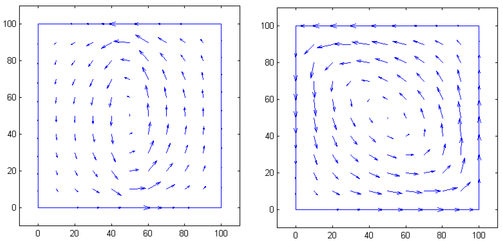
The salt water with higher concentration diffuses towards the bottom under the influence of the gravity. Meanwhile the fresh water diffuses towards the top. The interface between the sea water and fresh water evolves from vertical direction to horizontal direction. After about 300 days, the fluid is in equilibrium and the evolution stops.
Figure 2 shows the flux field
at the initial time and at time
days. One can observe the interface motion in
Figure 3. The refined elements are located in the neighborhood of the interface and follow the movement of the interface motion.
We start with a uniform mesh of
volume elements. An adaptive mesh is applied at each time step, taking into account the variations of the concentration
u. We present the numerical results for the concentration in
Figure 3. Since the mesh is coarse at the beginning, we choose
to create a finer mesh. Additionally, we choose
to balance refinement and merge. At
days, the number of elements is large enough, so we that set
to reduce the number of volume elements to be refined and set
. Since the evolution is slow from
to the end, we choose
and
.
Table 2 shows the number of volume elements of the adaptive mesh at different times. In the early stage, the adaptive mesh has a small number of elements. At the end, the refined mesh in the interface region is approximately a uniform mesh of
.
In
Figure 4, we compare the CPU times with different meshes with respect to the time in the physical flow process. We consider three uniform meshes with respectively 100 (
), 400 (
) and 1600 (
) volume elements and an adaptive mesh. We observe that using an adaptive mesh saves CPU time comparing to the uniform mesh
case at the same flow process time.
3.4. Mass Conservation
We discuss the conservation of mass in this subsection. We first check the mass conservation in the partial differential equation system. We integrate the transport Equation (3) on
for a given
t, in the case that
:
so that
We recall that that
and
on
, which we substitute in (20) to deduce
so that the system possesses the mass conservation property. Next, we check the mass is also conserved by the numerical scheme. We add up the semi-implicit discrete Equations (14) on all volume elements
, and set
to obtain: -4.6cm0cm
We define the total mass at the time
by
. Using the local conservation of the discrete fluxes on the interior edges (14) and the homogenous Neumann boundary condition, we deduce that:
which shows the fact that the mass is conserved in our algorithm. We check in
Table 3 that, in the simulation, the mass is indeed conserved. The total mass at the initial time is
.
3.5. Test Case Proposed by Henry
Henry’s problem describes the case that the sea water front advances in a confined aquifer which is initially filled with fresh water. It is one of the most standard tests for variable density flow in groundwater.
Mathematically, Henry’s problem [
4] is defined as System (1) in space domain
D together with the initial conditions such that
and that the pressure
satisfies
for all
. The source term is such that
. Suppose that
y is
y-coordinate; then the boundary conditions are given by
We consider the space domain
, and
days.
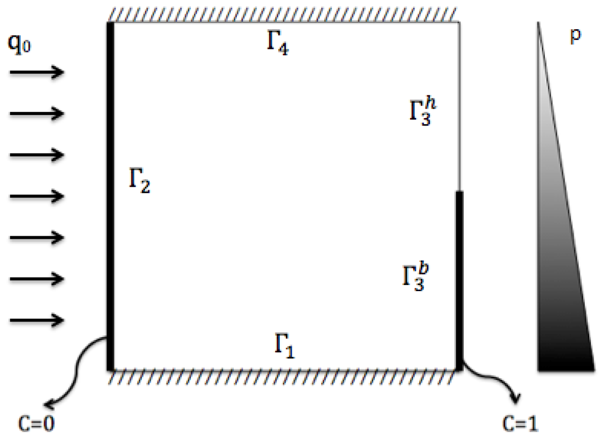
Figure 5 shows the configuration of the boundary conditions. The parameters are given in
Table 4.
Salt water invades from the right side, and fresh water with density
flows in from the left side at a constant rate. Therefore, the concentration near the coast increases in time. The interface between freshwater and saltwater flowing from the lower right corner has a large slope at first (left in
Figure 6), but gradually decreases as the salinity enters the domain (right in
Figure 6). The simulation in
Figure 7 shows how salt water invades the confined aquifer.
We start with a uniform mesh with
square elements. The variation of the concentration
u stays in a region around the boundary
, i.e.,
. We refine the mesh according to the variation of
u and choose
to keep the refine-list long enough at each time step and set
to keep the simulation process stable.
Table 5 presents the number of elements of the adaptive mesh at various times. In the adaptive mesh, the smallest volume elements have the same diameter as the volume elements in the uniform mesh
. The number of elements is one of the reasons why the CPU time by using adaptive mesh is smaller than the CPU time corresponding to the uniform mesh
. The evolutions of the CPU times with respect to the time in the flow process in different meshes are shown in
Figure 8. As a conclusion, by using an adaptive mesh, we keep the same precision over the high variation region and we save CPU time, especially in the case of Henry’s problem.
4. Density Driven Flow Coupled with Heat Transfer
In this section, we also introduce heat transfer. We perform computations for a test problem proposed in the SEAWAT documentation [
8].
SEAWAT is a computer program for simulating the transport of solutes and heat [
8]. It is a combination of MODFLOW and MT3DMS, which calculates the flow with MODFLOW and simulates solute transport with MT3DMS. SEAWAT can use both explicit and implicit time schemes to couple flow and solute transport.
The SEAWAT code is based on the finite difference method to solve systems of equations for variable density flow. MODFLOW and MT3DMS are both based on the finite difference method using a cell centered grid. The dependent variables obtained by the finite difference method represent the mean value in each cell (assuming that it is given at the center of the cell). Note that SEAWAT, MODFLOW, and MT3DMS use the same block center grid.
We propose a single code by using the generalized finite volume method SUSHI. The structure is simpler because it deals with one code rather than combining two separate codes with each other. Let us quote an article by [
9] about the study of related problems using the Voronoi box-based finite volume method.
4.1. Partial Differential Equation System
4.1.1. Variable Density Groundwater Equation
We consider a model in SEAWAT and present below the case of a single species. The space domain is given by the rectangle
. We apply the following variable density groundwater flow equation
in
, where
h [m] is the equivalent fresh water head,
[1/m] is the specific storage, defined as the water volume released from the storage per unit decline of
h,
[kg/m
] is the fluid density,
is the porosity,
[d
] is a source/sink of the fluid with density
. Equation (
12) is a generalized form of Equation (1). The velocity
[m/d] is given by Darcy’s law:
where
[kg/(m·s)] is the dynamic viscosity and
is the reference viscosity,
[m/d] is the hydraulic conductivity tensor,
is the density when the fluid is at the reference concentration
[kg/m
] and the reference temperature
[
C]. Additionally,
z [m] is the elevation, such that
.
4.1.2. The Fluid Density
We refer to Hughes and Sanford [
10] for the following equation for the transport of the solute species,
The concentration of the species can affect the fluid density. We reformulated here the term
by using the height of a water column
l of density
. The variable
l is related to the pressure by
where
. We rewrite the formula for the fluid density
as a function of the concentration
u, the temperature
and the hydraulic head
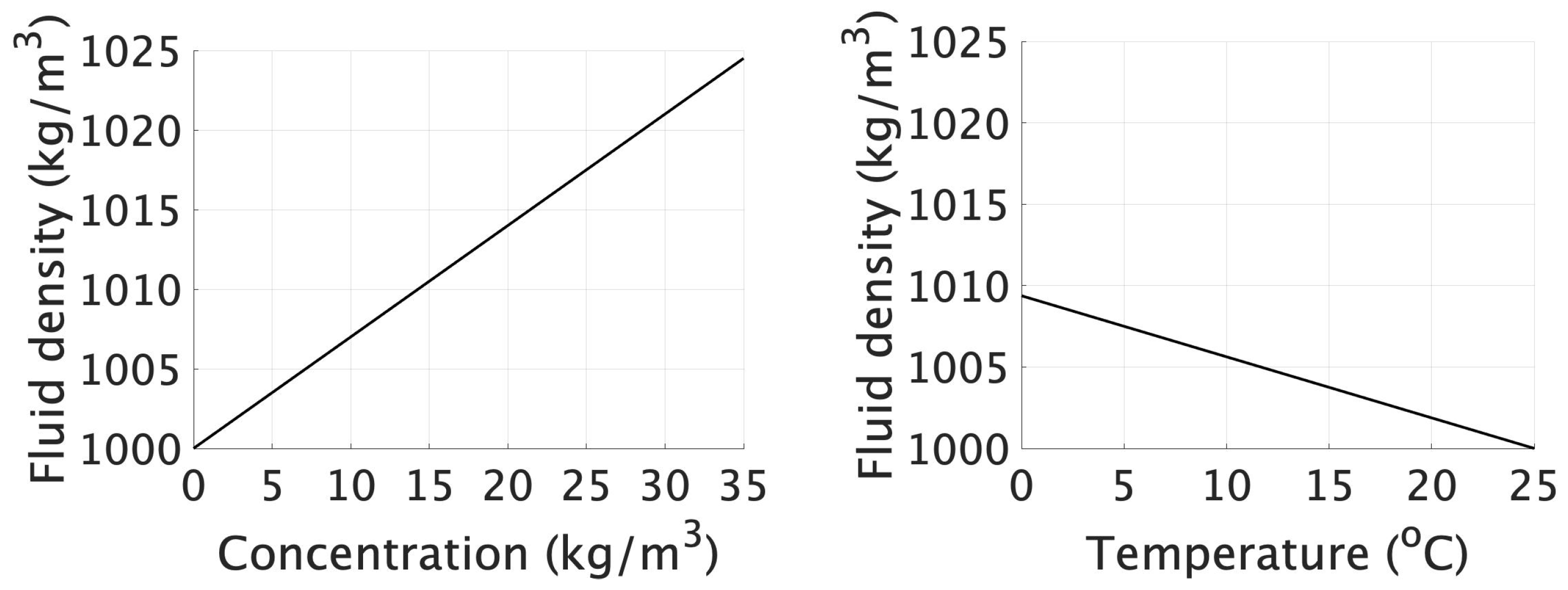
h as
An illustration of of the fluid density
is given in
Figure 9.
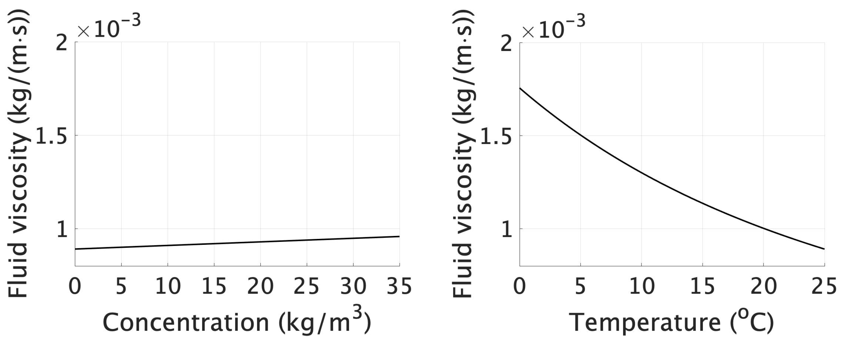
4.1.3. The Dynamic Fluid Viscosity
In [
3], the dynamic viscosity is considered as a function of temperature and the solute concentration is given. We ignore the dependence of the viscosity on the fluid pressure. A general formula for fluid viscosity as a function of concentration and temperature is given by
In many temperature ranges, the linear approximation does not adequately represent the effect of temperature on dynamic viscosity. For this reason, we have introduced an alternative formula for dynamic viscosity, namely
There are many ways to express
as a function of temperature. Here, the following relationship between viscosity and temperature is used.
where
,
,
and
are positive constants (cf. C.I. Voss [
11]). It yields the following formula for the dynamic viscosity:
An illustration of the fluid viscosity
is given in
Figure 10.
4.1.4. The Solute Transport Equation and the Heat Transport Equation
The solute transport in groundwater is described by an advection–dispersion equation. We apply the general form
in
, where
[kg/m
3] is the bulk density,
[m
3/kg] is the distribution coefficient for salinity,
[m
2/d] is the diffusion coefficient and
[m] is the dispersivity tensor. We remark that the dispersion tensor is defined by
where
and
are given in
Table 6.
Next, we apply the heat transport equation in Thorne et al., 2006 [
12].
in
, where
[m
3/kg] is the temperature distribution coefficient and
[m
2/d] is the bulk thermal diffusivity. We numerically solve the system of Equations (22), (23), (26) and (28) together with the boundary conditions
where
and where
,
and
correspond to Dirichlet boundary conditions and
,
and
correspond to Neumann boundary conditions for the hydraulic head
h, the concentration
u, and the temperature
, respectively. We denote initial conditions by
4.2. Numerical Approximation
We remark that from [
8], the derivatives
,
,
in the Equation (24) and
in the Equation (25) are constants. We set
and
and present below a numerical scheme corresponding to the system (22)–(28) with the boundary condition (29) and the initial conditions (30).
4.2.1. Numerical Approximation of the Fluxes
We plug Darcy’s law (23) into (22) and integrate over the volume element
p for each
to obtain
The diffusion flux
is approximated by
, such that
for
where
are defined as
and
is given as in (9).
We integrate Equations (26) and (28) over the volume element
p for each
, to obtain
We then define the numerical fluxes
and
to approximate the fluxes
and
, respectively. In view of the SUSHI method, we present the discrete fluxes
and
as:
where
and
where
4.2.2. Numerical Scheme
The discrete initial conditions are given by
Next, we present the discretized problem. For all :
We suppose that
,
,
and
are already known and search for
such that
where
,
,
, and
are computed as (30), (40) and (41), respectively. When
, we omit the term
in Equation (35). The velocity
approximates
at time
and is given by
where
and
Knowing
,
, we search for
such that
Knowing
,
, we search for
such that
where
and
are given by the upwind scheme
for each time step
n.
The discrete fluxes and are defined by (33) and (34), respectively. The three Equations (36), (43) and (47) are the conservation of the discrete fluxes on the interior edges.
4.3. Numerical Tests
We consider the model problem developed in the SEAWAT [
8] that is a two-dimensional cross section of a confined coastal aquifer initially filled with seawater at temperature 5
C, which corresponds to
,
and
. Along the left boundary, warm freshwater with a temperature of
is injected into the coastal aquifer to represent the flow from the inland area. Warm freshwater flows to the right and flows into a vertical ocean boundary. At the ocean boundary, hydrostatic pressure conditions based on the fluid density calculated from the salinity of seawater at 5
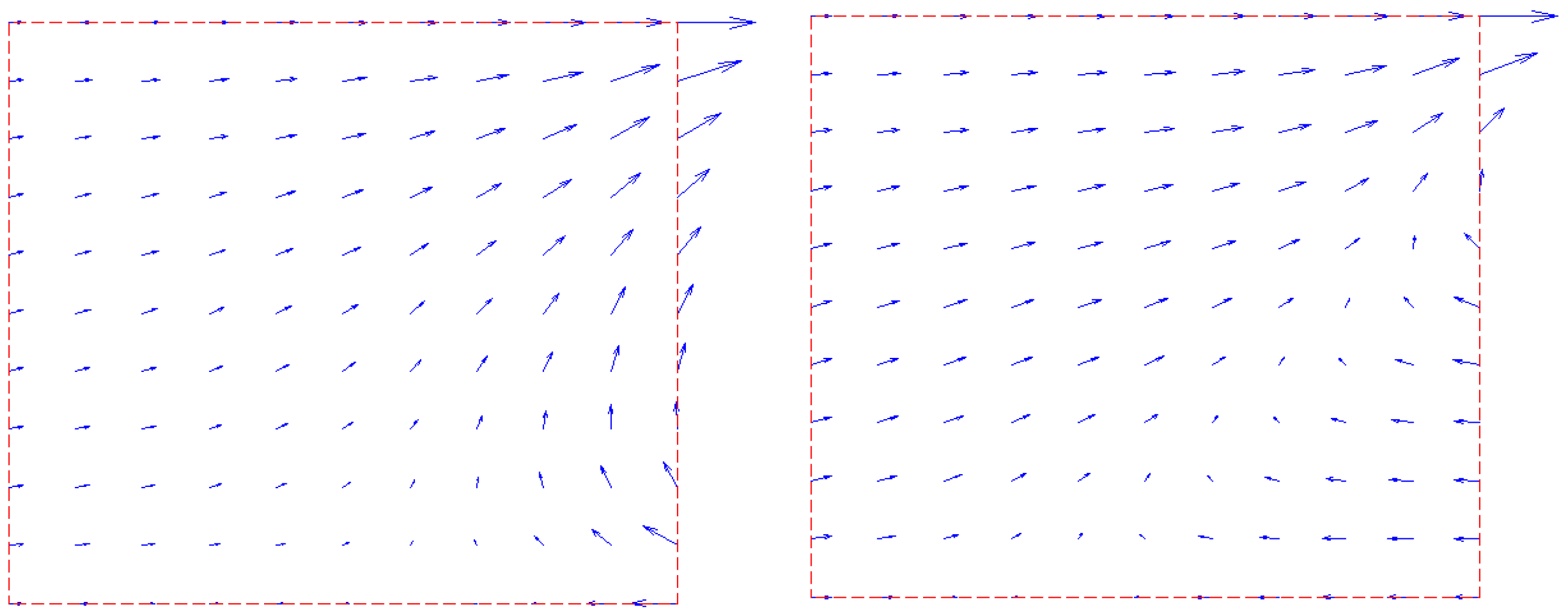
C were set. No flow boundary conditions are set for the upper and lower boundaries. Because of the gravity and the no flow boundary conditions the velocities differ at the top, bottom, and middle of the aquifer. At the bottom part, the flow is slow, so the concentration and temperature values do not change much. At the top part, the flow is fast, and the concentration and temperature values change rapidly.
The boundary condition on the sea water boundary is given by
, where
is the seawater density and the elevation
z is such that
. The average flux velocity on the boundary
is given by
with
. We have that
, and the parameters are given in
Table 6.
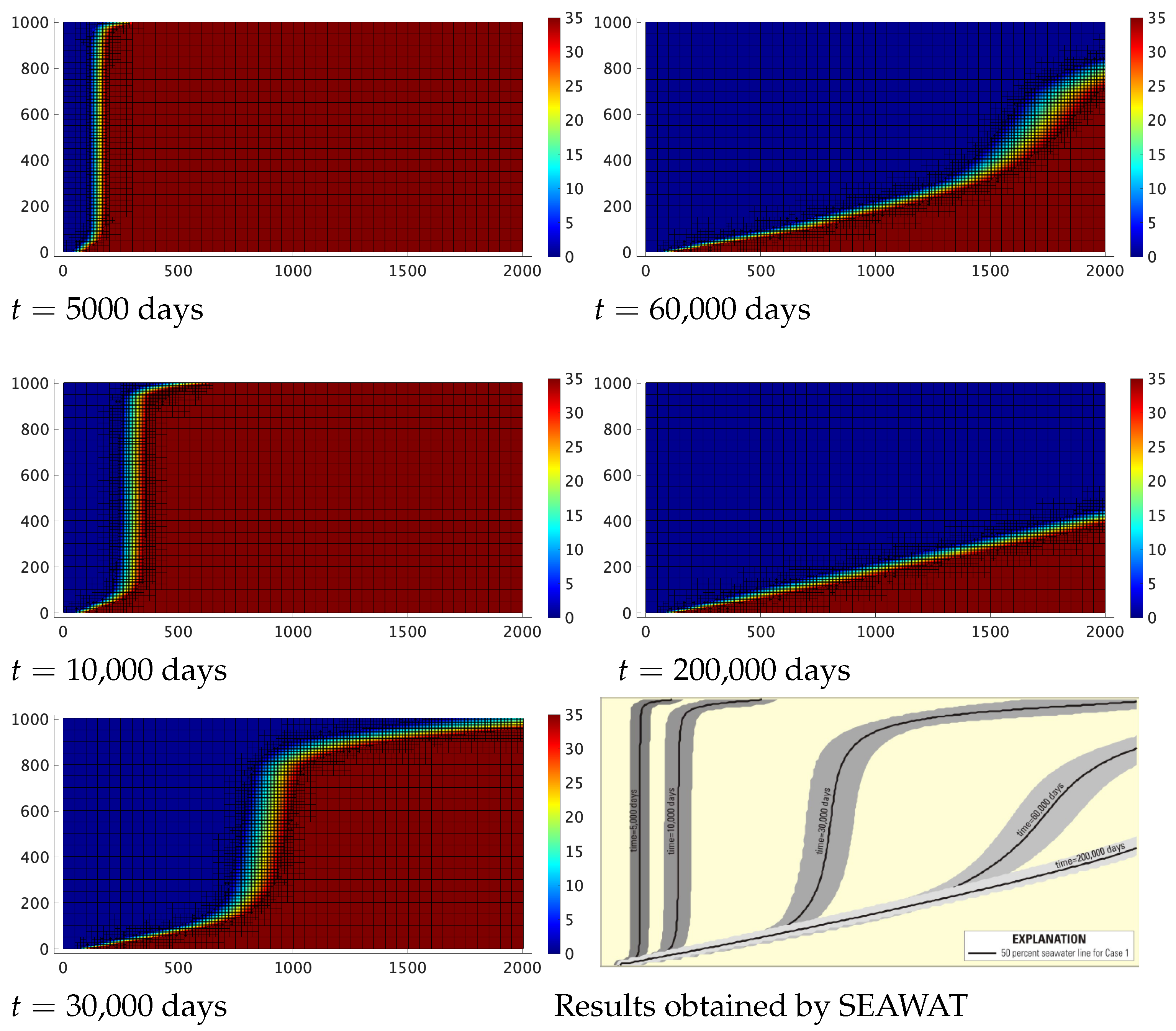
The adaptive mesh is efficient in this problem, since the variations of the concentration and of the temperature only take place in their interface areas, respectively. We present numerical simulations in three cases. For test cases 1 and 2 below, we neglect the heat transfer equation and consider the mesh refinement to be based on the variation of the concentration
u (
Figure 11 and
Figure 12). In test case 3, the interfaces of the concentration and of the temperature do not advance with the same speed, so that we perform a first computation with the refinement based on the variation of the concentration (
Figure 13) and a second time computation with the refinement based on the variation of the temperature in order to present the results on the temperature profiles (
Figure 14).
We start from a uniform square mesh to discretize the domain where and . We fix and to keep the simulation process stable; we observe that the mesh is mostly refined in the neighborhood of the interface.
4.3.1. Test Cases 1 and 2 without Heat Transfer
In the first 2 test cases, we consider different expressions of the fluid density
and suppose that the fluid viscosity
is constant. We neglect the heat transfer equation and consider the system
We apply the Equations (35), (39) and (42) for the numerical simulations.
Test case 1: We suppose that the fluid density only depends on the concentration
u and can be rewritten as
Figure 11 shows the evolution of the concentration
u in time in test case 1.
Test case 2: In test case 2, we suppose that the density
is a linear function of concentration
u and of temperature
:
equals to
and it indicates that the fluid density will decrease as the temperature increases.We suppose that the temperature
is a linear function of the concentration
u:
where
,
,
kg/m
and
kg/m
.
Figure 12 shows the evolution in time of the concentration
u in this test case.
We compare our results to those in SEAWAT [
8] in the
Figure 11 and
Figure 12, and by a uniform piece of code, we obtain results which look very close to the results of SEAWAT. We then compare the numerical results in the two cases and find out that in test case 2, the front advancement speed is lower and that the transition front’s width is thinner due to the influence of the temperature.
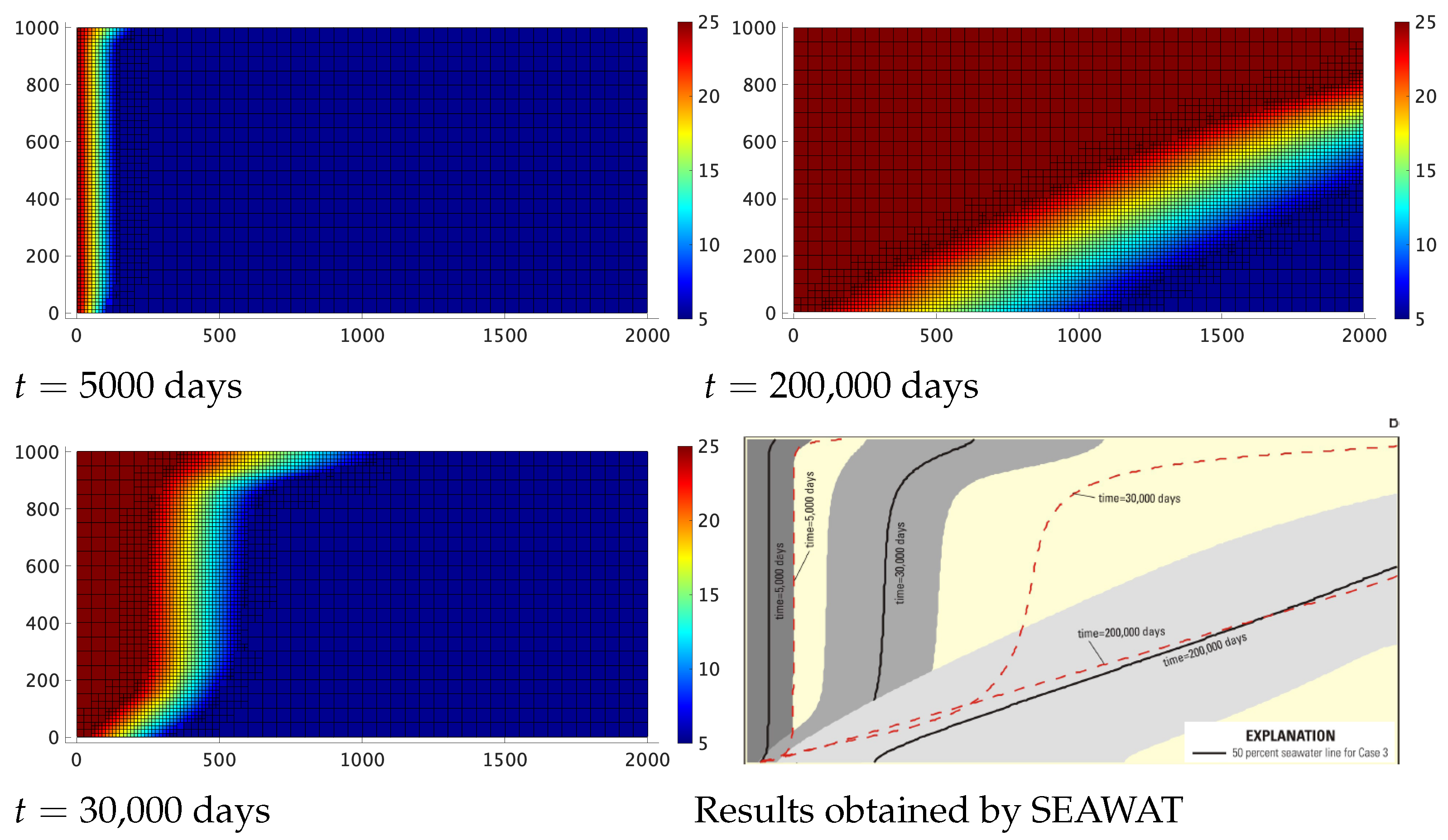
4.3.2. Test Case 3
In test case 3, we take the heat transfer equation into account. In this case, the fluid density
is given by (
14) and the viscosity
is given by (
15). The transient motion of the concentration and that of the temperature are shown in the
Figure 13 and
Figure 14. In
Figure 13, an adaptive mesh corresponding to the concentration variation is used. Meanwhile, we perform the simulation for a second time with an adaptive mesh corresponding to the temperature in
Figure 14.
We observe that the concentration transition zone and temperature transition zone do not advance at the same speed; and the width of the transition fronts of the concentration u is thicker in test case 3 than in the previous 2 cases.
5. Conclusions
In this article, the generalized finite volume method SUSHI on an adaptive mesh is applied to simulate density-driven flow in a porous medium.
HydroExpert, the small hydrology company with whom we used to work, only used square mesh elements for the space discretization; these elements coincided with data coming from physical measurements. This led us to also apply a standard square mesh in space dimension 2. We proposed a criterion for selecting the volume elements to be refined based on the variability of selected geophysical quantities, such as the concentration. It turns out that the mesh is mostly refined along the interface between fresh water and sea water so that we save CPU time while maintaining the same accuracy in interface regions.
Refining any part of the domain will result in a non-matching mesh. The finite difference method or the standard finite volume method cannot be applied to the non-matching mesh, but the SUSHI method can be applied. Moreover, the SUSHI method can handle problems with anisotropic and inhomogeneous diffusion tensors.
In the simulations of the SEAWAT model, we proposed a single algorithm that is simpler than the SEAWAT software, which combines MODFLOW to compute the flow with MT3DMS to simulate the solute-transport. Taking all this into account, the method that we propose is an effective option for simulations related to density driven flow in porous media.


