
Applicability of Different Double-Layer Models for the Performance Assessment of the Capacitive Energy Extraction Based on Double Layer Expansion (CDLE) Technique


Abstract
:1. Introduction
2. Materials and Methods
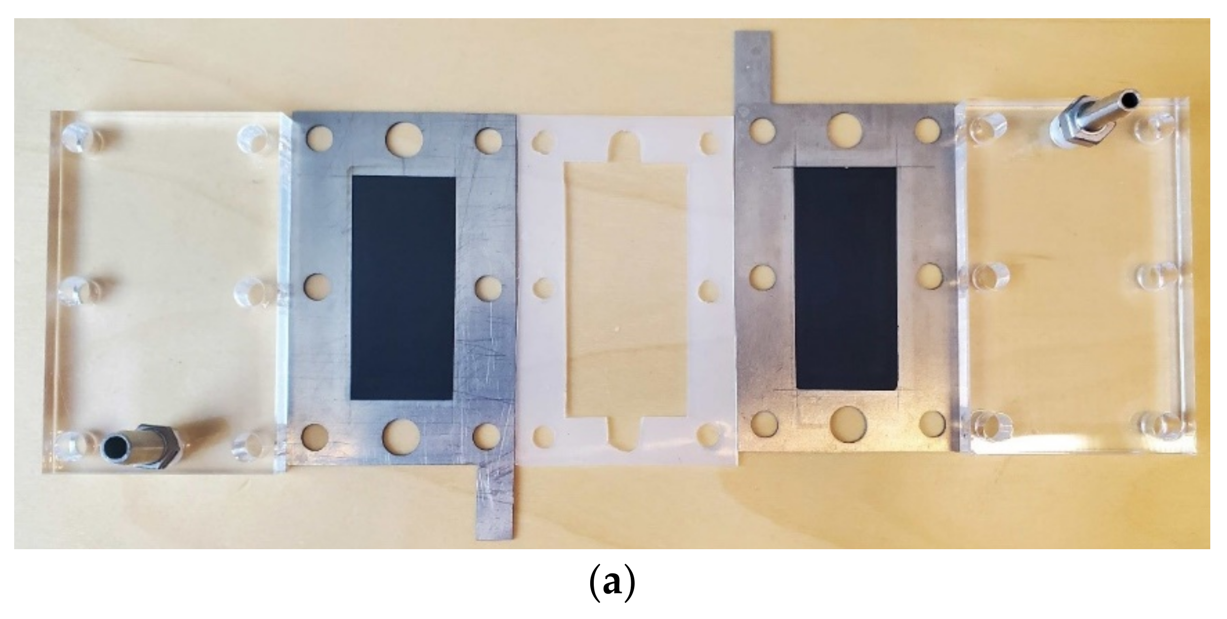
2.1. Materials
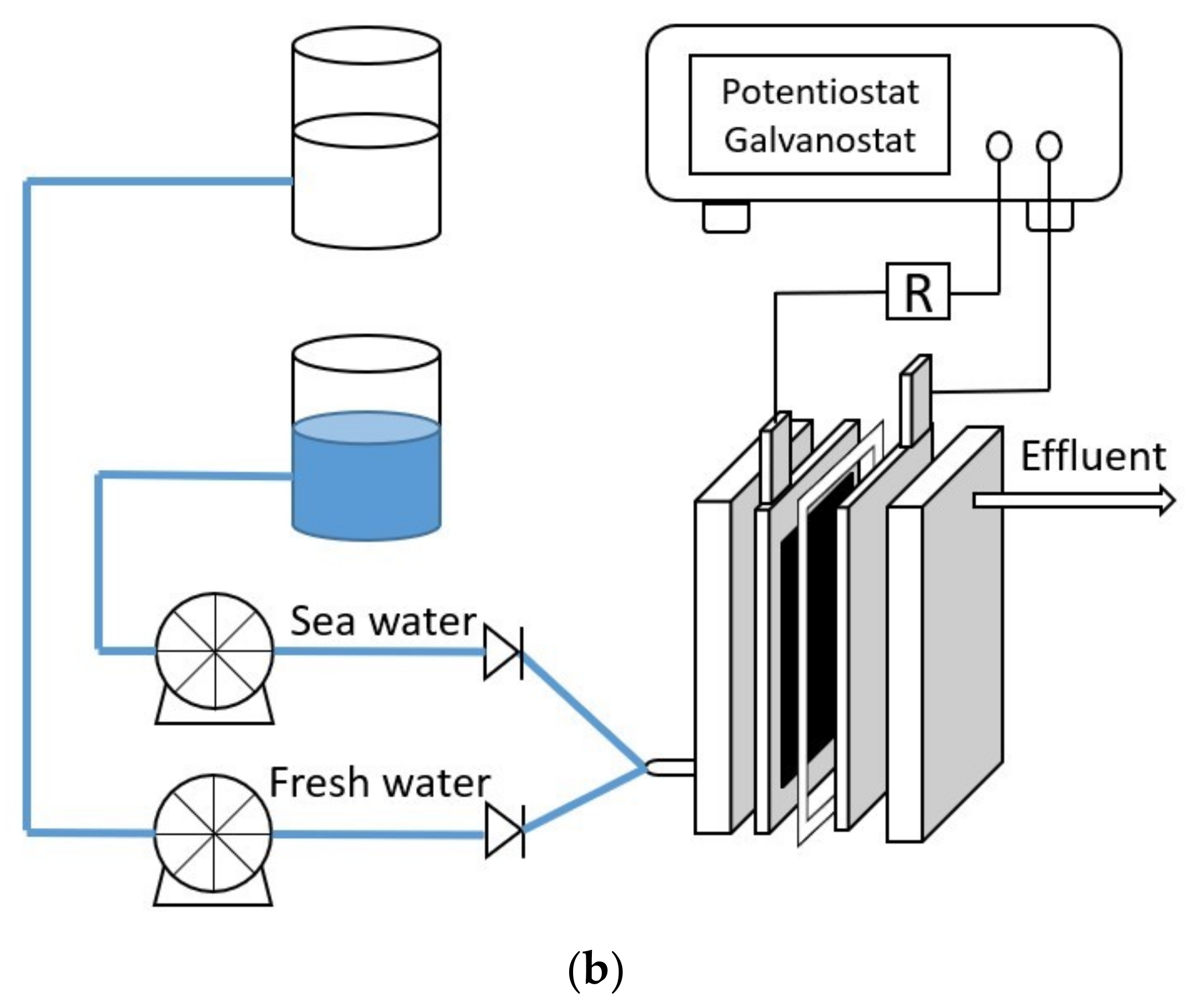
2.2. Operations
3. Theory of Electrical Double Layers
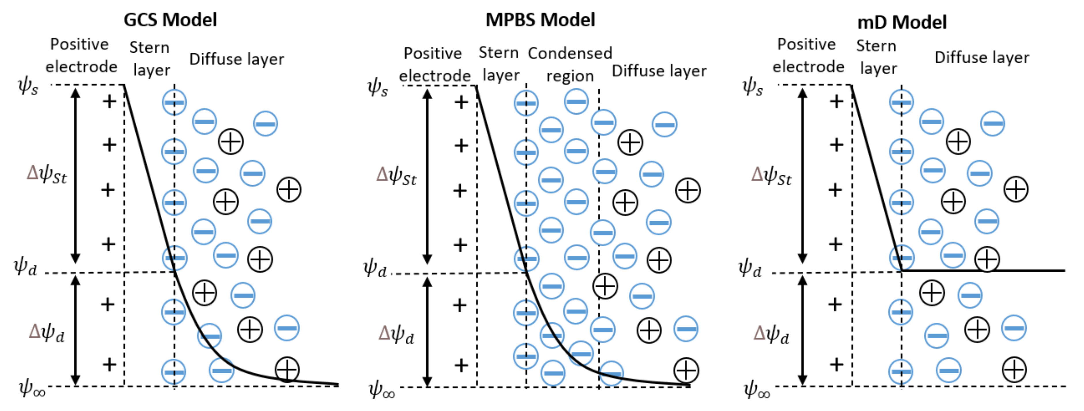
3.1. Gouy–Chapmann–Stern Model
3.2. Modified Poisson–Boltzmann–Stern Model
3.3. Modified Donnan Model
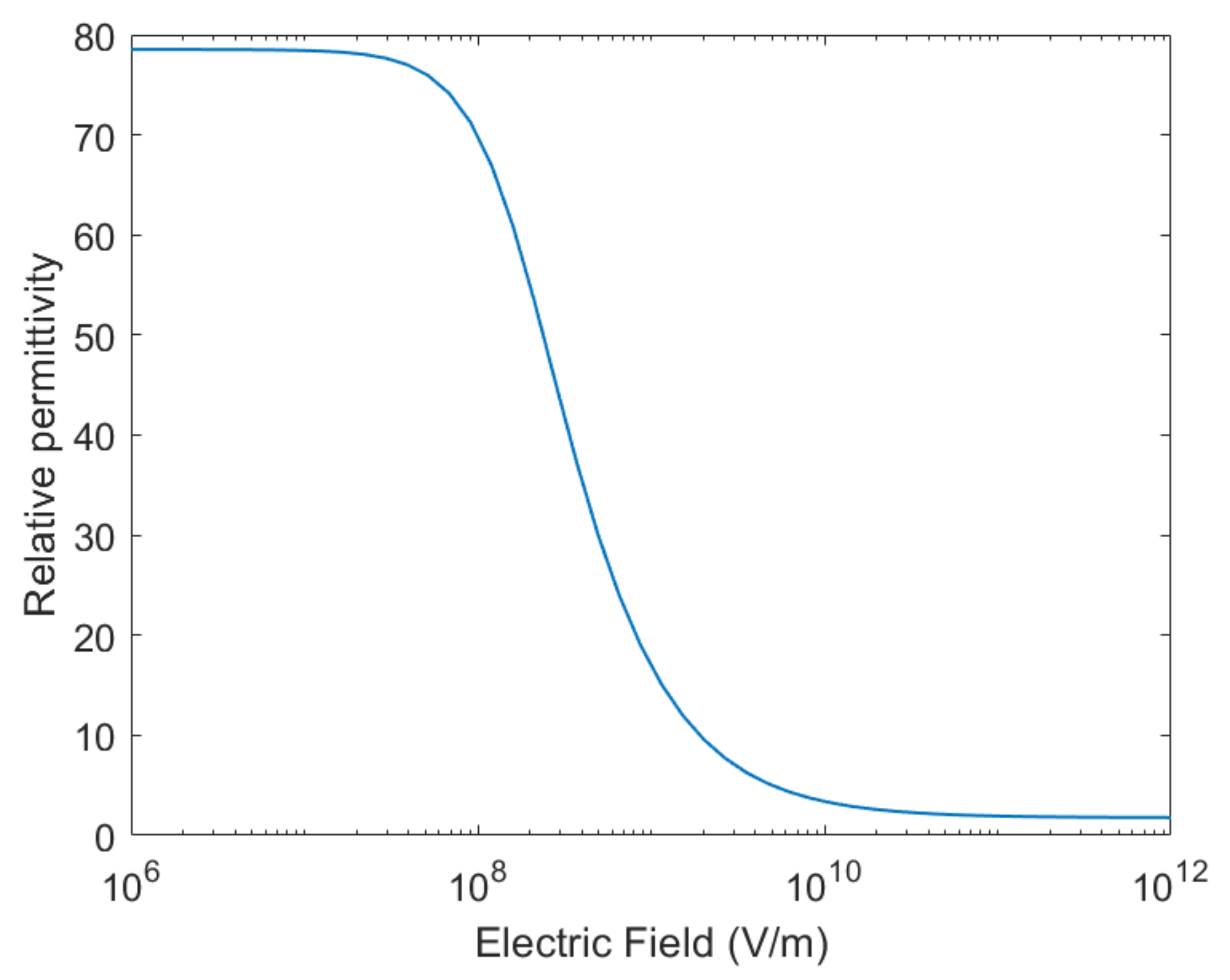
3.4. Booth Correction of Dielectric Permittivity
4. Experimental Results and Model Applications
4.1. Gouy–Chapmann–Stern Model
4.2. Modified Poisson–Boltzmann–Stern Model
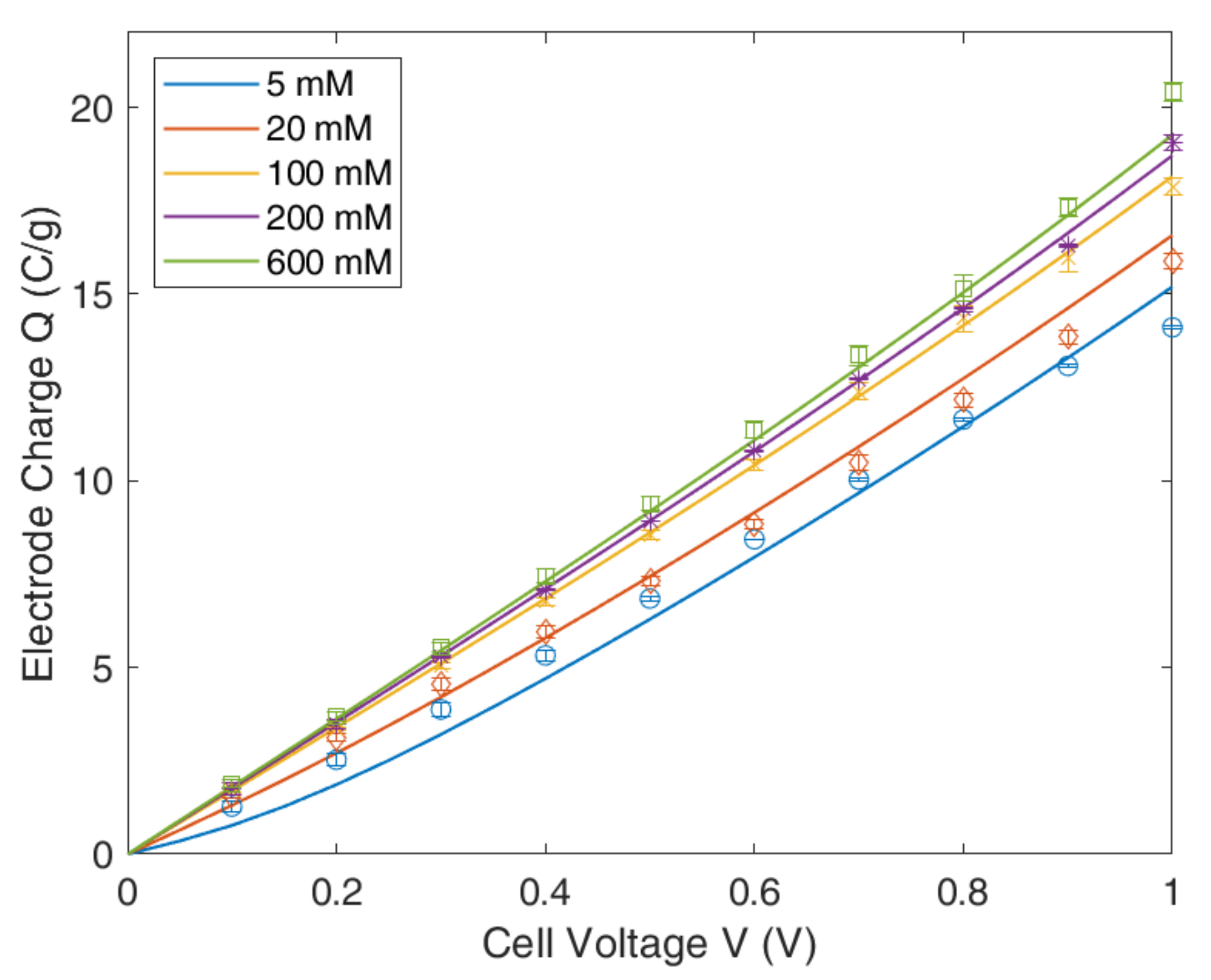
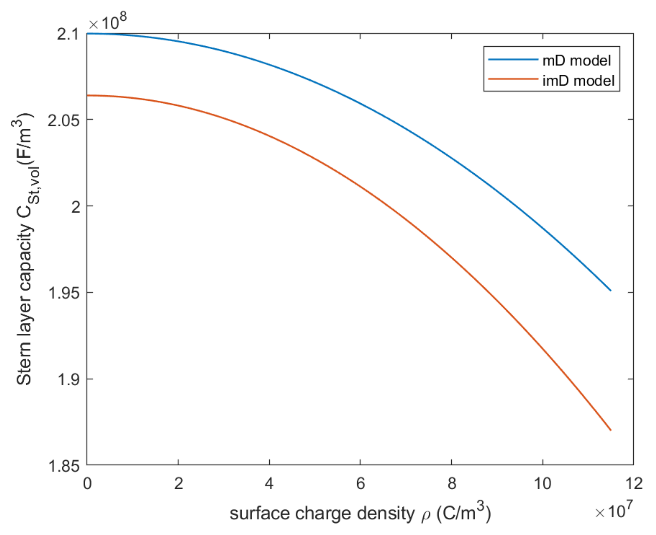
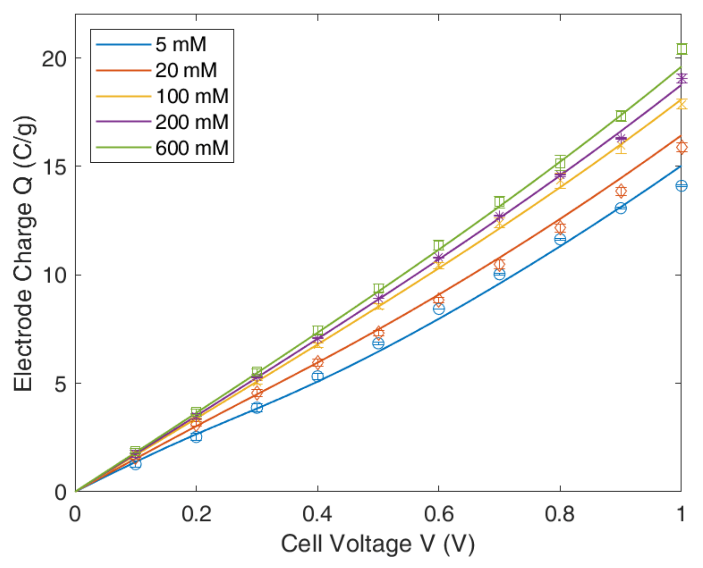
4.3. Modified Donnan Model
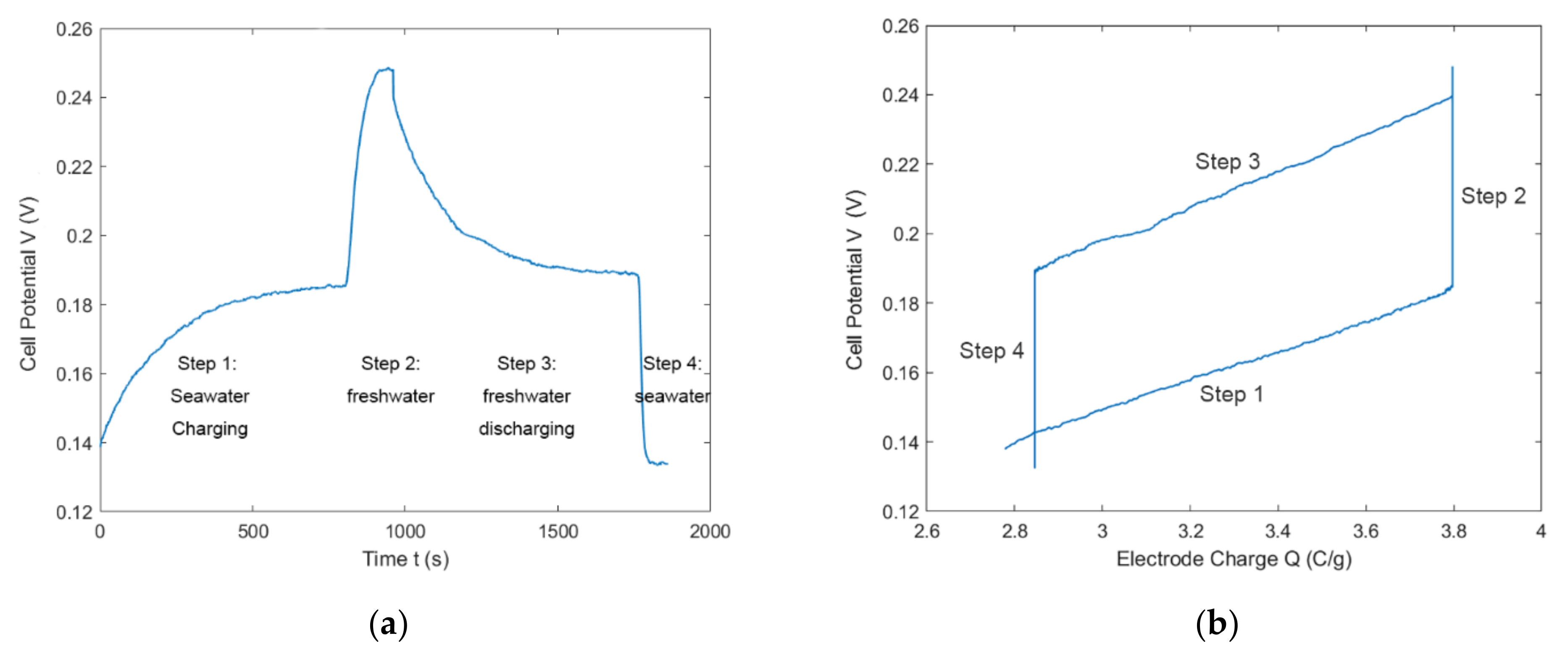
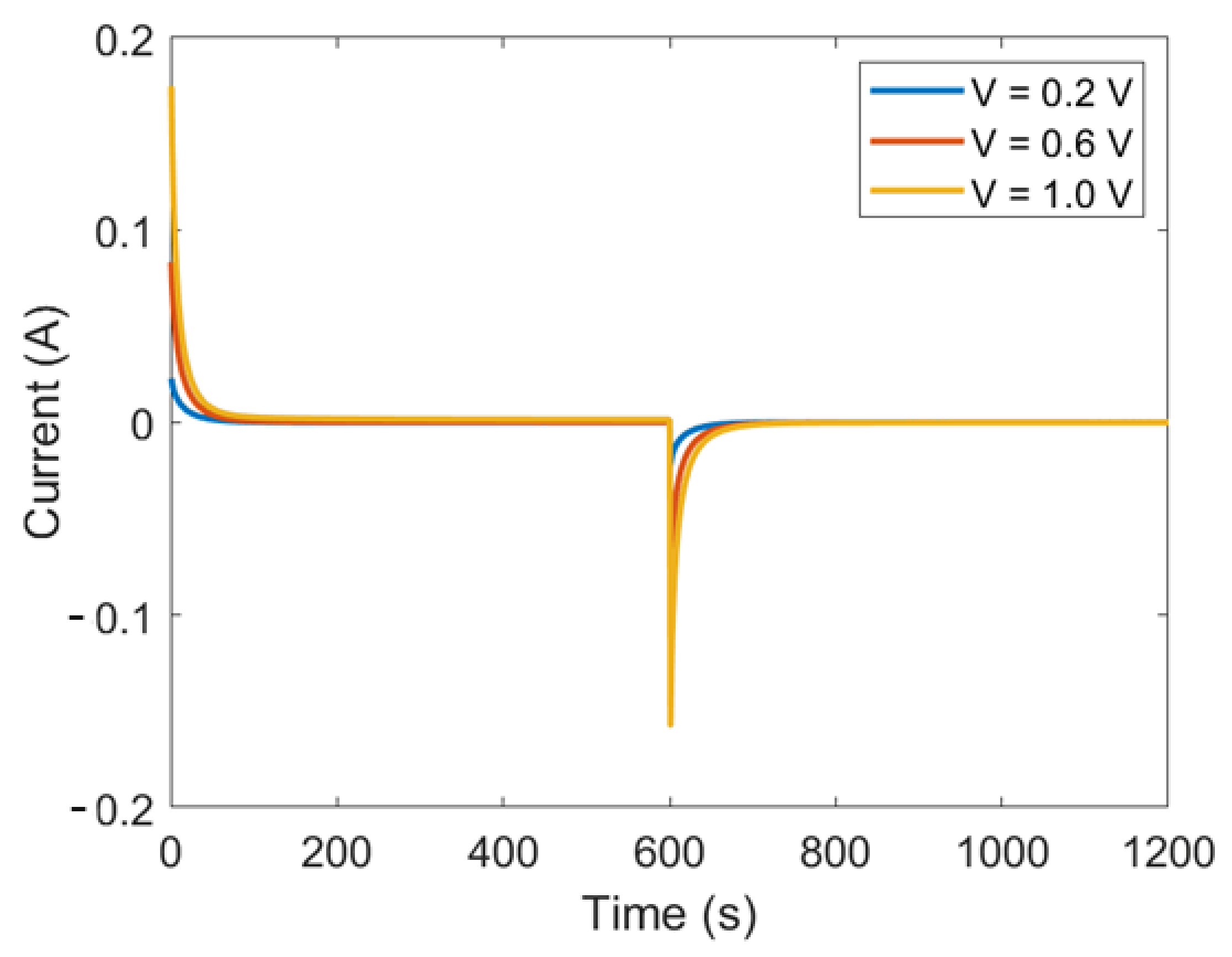
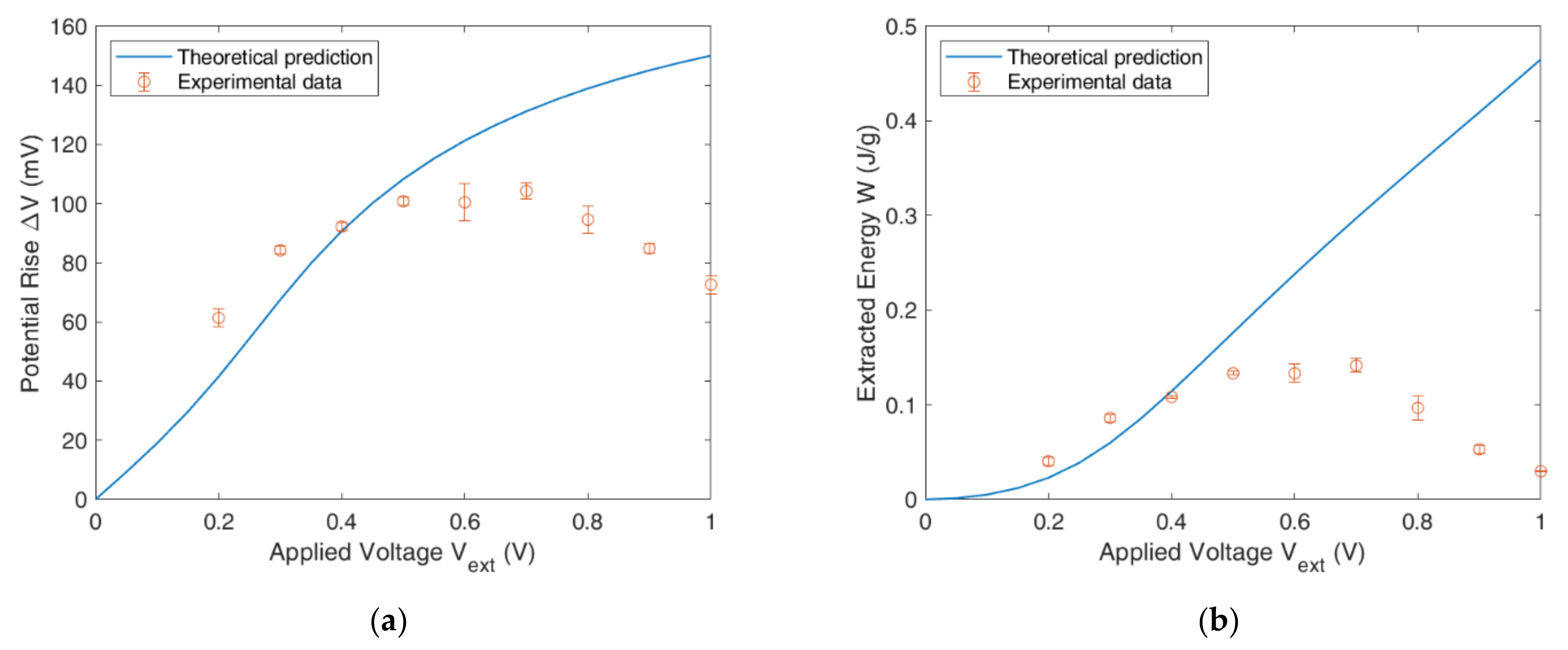
4.4. Full CDLE Experiment
5. Conclusions
Author Contributions
Funding
Institutional Review Board Statement
Informed Consent Statement
Data Availability Statement
Acknowledgments
Conflicts of Interest
Nomenclature
| CapMix | Capacitive mixing |
| CDP | Capacitive energy extraction based on Donnan Potential |
| CDLE | Capacitive energy extraction based on Double Layer Expansion |
| SE | Soft Electrode |
| EDL | Electric double layer |
| PB | Poisson Boltzmann |
| GCS | Gouy–Chapman–Stern |
| MPBS | Modified Poisson–Boltzmann–Stern |
| mD | modified Donnan |
| Specific surface area | |
| Microporous surface area measurement | |
| Total volume of pores | |
| Pore thickness | |
| Average pore diameter | |
| Equilibrium electrode charge per mass, C/g | |
| Electric current, A | |
| Measured current, A | |
| Leakage current, A | |
| Mass of total electrodes, g | |
| Applied voltage, V | |
| Cell potential, V | |
| Potential increase due to the double layer expansion, V | |
| External resistance, Ω | |
| Extracted energy, J/g | |
| Electrolyte concentration, mm | |
| Electrolyte concentration of freshwater, mol/m3 | |
| Electrolyte concentration of seawater, mol/m3 | |
| micropore total ion concentration, mol/m3 | |
| number concentration of the ith species in diffuse layer, 1/m3 | |
| number concentration of the ith species at the bulk solution, 1/m3 | |
| number concentration of ith species in the micropores of the electrode, 1/m3 | |
| elementary charge, C | |
| valence of the ith species | |
| Boltzmann constant, J/K | |
| free space permittivity, F/m | |
| relative permittivity of the electrolyte solutions | |
| electric potential, V | |
| surface potential, V | |
| electric potential drop across the stern layer, V | |
| electric potential difference across the diffuse layer, V | |
| surface charge density, C/m2 | |
| total differential capacitance of the double layer | |
| differential capacitances of the stern layer, F/m2 | |
| differential capacitances of the diffuse layer, F/m2 | |
| average excluded volume per ion, m3 | |
| d | spacing of counterions near a highly charged surface, m |
| Debye length, m | |
| Bjerrum length, m | |
| volumetric charge density, C/m3 | |
| excess chemical potential, kT | |
| volumetric capacitance of the Stern layer, F/ m3 | |
| volumetric capacitance of the Stern layer (low charge limit), F/ m3 | |
| Parameter to describe nonlinear part of Stern capacity, F∙m3/mol2 | |
| E | energy parameter, kT mol/m3 |
| size of micropore, m | |
| index of refraction of the electrolyte at zero electric field frequency | |
| dipole moment of the solvent molecule and in the case of water, D(Debye) | |
| effective specific electrode area, m2/g |
References
- Shirzad, M.; Karimi, M.; Abolghasemi, H. Polymer inclusion membranes with dinonylnaphthalene sulfonic acid as ion carrier for Co(II) transport from model solutions. Desalin. Water Treat. 2019, 144, 185–200. [Google Scholar] [CrossRef]
- De Medeiros, A.D.M.; da Silva, C.J.G.; de Amorim, J.D.P.; do Nascimento, H.A.; Converti, A.; Costa, A.F.D.; Sarubbo, L.A. Biocellulose for Treatment of Wastewaters Generated by Energy Consuming Industries: A Review. Energies 2021, 14, 5066. [Google Scholar] [CrossRef]
- Ozcan, H.G.; Hepbasli, A.; Abusoglu, A.; Anvari-Moghaddam, A. Advanced Exergy Analysis of Waste-Based District Heating Options through Case Studies. Energies 2021, 14, 4766. [Google Scholar] [CrossRef]
- Pattle, R. Production of electric power by mixing fresh and salt water in the hydroelectric pile. Nature 1954, 174, 660. [Google Scholar] [CrossRef]
- Boon, N.; van Roij, R. ‘Blue energy’ from ion adsorption and electrode charging in sea and river water. Mol. Phys. 2011, 109, 1229–1241. [Google Scholar] [CrossRef] [Green Version]
- Post, J.W.; Hamelers, H.V.M.; Buisman, C.J.N. Energy recovery from controlled mixing salt and fresh water with a reverse electrodialysis system. Environ. Sci. Technol. 2008, 42, 5785–5790. [Google Scholar] [CrossRef]
- Achilli, A.; Childress, A.E. Pressure retarded osmosis: From the vision of Sidney Loeb to the first prototype installation. Desalination 2010, 261, 205–211. [Google Scholar] [CrossRef]
- Loeb, S. Osmotic Power-Plants. Science 1975, 189, 654–655. [Google Scholar] [CrossRef] [Green Version]
- Weinstein, J.N.; Leitz, F.B. Electric power from differences in salinity: The dialytic battery. Science 1976, 191, 557–559. [Google Scholar] [CrossRef]
- Yip, N.Y.; Elimelech, M. Comparison of energy efficiency and power density in pressure retarded osmosis and reverse electrodialysis. Environ. Sci. Technol. 2014, 48, 11002–11012. [Google Scholar] [CrossRef]
- Yip, N.Y.; Brogioli, D.; Hamelers, H.V.M.; Nijmeijer, K. Salinity Gradients for Sustainable Energy: Primer, Progress, and Prospects. Environ. Sci. Technol. 2016, 50, 12072–12094. [Google Scholar] [CrossRef] [PubMed]
- Kim, T.; Rahimi, M.; Logan, B.E.; Gorski, C.A. Harvesting Energy from Salinity Differences Using Battery Electrodes in a Concentration Flow Cell. Environ. Sci. Technol. 2016, 50, 9791–9797. [Google Scholar] [CrossRef]
- Brogioli, D. Extracting Renewable Energy from a Salinity Difference Using a Capacitor. Phys. Rev. Lett. 2009, 103, 058501. [Google Scholar] [CrossRef]
- Sales, B.B.; Saakes, M.; Post, J.W.; Buisman, C.J.N.; Biesheuvel, P.M.; Hamelers, H.V.M. Direct Power Production from a Water Salinity Difference in a Membrane-Modified Supercapacitor Flow Cell. Environ. Sci. Technol. 2010, 44, 5661–5665. [Google Scholar] [CrossRef] [PubMed]
- La Mantia, F.; Pasta, M.; Deshazer, H.D.; Logan, B.E.; Cui, Y. Batteries for Efficient Energy Extraction from a Water Salinity Difference. Nano Lett. 2011, 11, 1810–1813. [Google Scholar] [CrossRef]
- Ahualli, S.; Jimenez, M.L.; Fernandez, M.M.; Iglesias, G.; Brogioli, D.; Delgado, A.V. Polyelectrolyte-coated carbons used in the generation of blue energy from salinity differences. Phys. Chem. Chem. Phys. 2014, 16, 25241–25246. [Google Scholar] [CrossRef] [PubMed] [Green Version]
- Iglesias, G.R.; Fernandez, M.M.; Ahualli, S.; Jimenez, M.L.; Kozynchenko, O.P.; Delgado, A.V. Materials selection for optimum energy production by double layer expansion methods. J. Power Sources 2014, 261, 371–377. [Google Scholar] [CrossRef]
- Nasir, M.; Nakanishi, Y.; Patmonoaji, A.; Suekane, T. Effects of porous electrode pore size and operating flow rate on the energy production of capacitive energy extraction. Renew. Energy 2020, 155, 278–285. [Google Scholar] [CrossRef]
- Iglesias, G.R.; Ahualli, S.; Fernandez, M.M.; Jimenez, M.L.; Delgado, A.V. Stacking of capacitive cells for electrical energy production by salinity exchange. J. Power Sources 2016, 318, 283–290. [Google Scholar] [CrossRef]
- Ahualli, S.; Fernandez, M.M.; Iglesias, G.; Delgado, A.V.; Jimenez, M.L. Temperature Effects on Energy Production by Salinity Exchange. Environ. Sci. Technol. 2014, 48, 12378–12385. [Google Scholar] [CrossRef] [PubMed] [Green Version]
- Zhao, R.; Biesheuvel, P.M.; Miedema, H.; Bruning, H.; van der Wal, A. Charge Efficiency: A Functional Tool to Probe the Double-Layer Structure Inside of Porous Electrodes and Application in the Modeling of Capacitive Deionization. J. Phys. Chem. Lett. 2010, 1, 205–210. [Google Scholar] [CrossRef]
- Brogioli, D.; Zhao, R.; Biesheuvel, P.M. A prototype cell for extracting energy from a water salinity difference by means of double layer expansion in nanoporous carbon electrodes. Energy Environ. Sci. 2011, 4, 772–777. [Google Scholar] [CrossRef] [Green Version]
- Brogioli, D.; Ziano, R.; Rica, R.A.; Salerno, D.; Kozynchenko, O.; Hamelers, H.V.M.; Mantegazza, F. Exploiting the spontaneous potential of the electrodes used in the capacitive mixing technique for the extraction of energy from salinity difference. Energy Environ. Sci. 2012, 5, 9870–9880. [Google Scholar] [CrossRef] [Green Version]
- Jimenez, M.L.; Fernandez, M.M.; Ahualli, S.; Iglesias, G.; Delgado, A.V. Predictions of the maximum energy extracted from salinity exchange inside porous electrodes. J. Colloid Interface Sci. 2013, 402, 340–349. [Google Scholar] [CrossRef]
- Fernandez, M.M.; Ahualli, S.; Iglesias, G.R.; Gonzalez-Caballero, F.; Delgado, A.V.; Jimenez, M.L. Multi-ionic effects on energy production based on double layer expansion by salinity exchange. J. Colloid Interface Sci. 2015, 446, 335–344. [Google Scholar] [CrossRef]
- Rica, R.A.; Ziano, R.; Salerno, D.; Mantegazza, F.; Bazant, M.Z.; Brogioli, D. Electro-diffusion of ions in porous electrodes for capacitive extraction of renewable energy from salinity differences. Electrochim. Acta 2013, 92, 304–314. [Google Scholar] [CrossRef] [Green Version]
- Rica, R.A.; Brogioli, D.; Ziano, R.; Salerno, D.; Mantegazza, F. Ions Transport and Adsorption Mechanisms in Porous Electrodes During Capacitive-Mixing Double Layer Expansion (CDLE). J. Phys. Chem. C 2012, 116, 16934–16938. [Google Scholar] [CrossRef]
- Biesheuvel, P.M.; Bazant, M.Z. Nonlinear dynamics of capacitive charging and desalination by porous electrodes. Phys. Rev. E 2010, 81, 031502. [Google Scholar] [CrossRef] [Green Version]
- Porada, S.; Bryjak, M.; van der Wal, A.; Biesheuvel, P.M. Effect of electrode thickness variation on operation of capacitive deionization. Electrochim. Acta 2012, 75, 148–156. [Google Scholar] [CrossRef] [Green Version]
- Porada, S.; Borchardt, L.; Oschatz, M.; Bryjak, M.; Atchison, J.S.; Keesman, K.J.; Kaskel, S.; Biesheuvel, P.M.; Presser, V. Direct prediction of the desalination performance of porous carbon electrodes for capacitive deionization. Energy Environ. Sci. 2013, 6, 3700–3712. [Google Scholar] [CrossRef] [Green Version]
- Porada, S.; Zhao, R.; van der Wal, A.; Presser, V.; Biesheuvel, P.M. Review on the science and technology of water desalination by capacitive deionization. Prog. Mater. Sci. 2013, 58, 1388–1442. [Google Scholar] [CrossRef] [Green Version]
- Bazant, M.Z.; Chu, K.T.; Bayly, B.J. Current-voltage relations for electrochemical thin films. Siam J. Appl. Math. 2005, 65, 1463–1484. [Google Scholar] [CrossRef] [Green Version]
- Wang, H.N.; Varghese, J.; Pilon, L. Simulation of electric double layer capacitors with mesoporous electrodes: Effects of morphology and electrolyte permittivity. Electrochim. Acta 2011, 56, 6189–6197. [Google Scholar] [CrossRef]
- Biesheuvel, P.M. Thermodynamic cycle analysis for capacitive deionization. J. Colloid Interface Sci. 2009, 332, 258–264. [Google Scholar] [CrossRef]
- Biesheuvel, P.M.; van Soestbergen, M. Counterion volume effects in mixed electrical double layers. J. Colloid Interface Sci. 2007, 316, 490–499. [Google Scholar] [CrossRef] [PubMed]
- Kilic, M.S.; Bazant, M.Z.; Ajdari, A. Steric effects in the dynamics of electrolytes at large applied voltages. I. Double-layer charging. Phys. Rev. E 2007, 75, 021502. [Google Scholar] [CrossRef] [Green Version]
- Biesheuvel, P.M.; Zhao, R.; Porada, S.; van der Wal, A. Theory of membrane capacitive deionization including the effect of the electrode pore space. J. Colloid Interface Sci. 2011, 360, 239–248. [Google Scholar] [CrossRef] [Green Version]
- Porada, S.; Weinstein, L.; Dash, R.; van der Wal, A.; Bryjak, M.; Gogotsi, Y.; Biesheuvel, P.M. Water Desalination Using Capacitive Deionization with Microporous Carbon Electrodes. ACS Appl. Mater. Inter. 2012, 4, 1194–1199. [Google Scholar] [CrossRef] [Green Version]
- Biesheuvel, P.M.; Porada, S.; Levi, M.; Bazant, M.Z. Attractive forces in microporous carbon electrodes for capacitive deionization. J. Solid State Electr. 2014, 18, 1365–1376. [Google Scholar] [CrossRef] [Green Version]
- Wang, H.N.; Pilon, L. Accurate Simulations of Electric Double Layer Capacitance of Ultramicroelectrodes. J. Phys. Chem. C 2011, 115, 16711–16719. [Google Scholar] [CrossRef]
- Booth, F. The dielectric constant of water and the saturation effect. J. Chem. Phys. 1951, 19, 391–394. [Google Scholar] [CrossRef]
- Booth, F. Dielectric constant of polar liquids at high field strengths. J. Chem. Phys. 1955, 23, 453–457. [Google Scholar] [CrossRef]
- Basu, S.; Sharma, M.M. Effect of Dielectric Saturation on Disjoining Pressure in Thin-Films of Aqueous-Electrolytes. J. Colloid Interface Sci. 1994, 165, 355–366. [Google Scholar] [CrossRef]
- Tansel, B.; Sager, J.; Rector, T.; Garland, J.; Strayer, R.F.; Levine, L.F.; Roberts, M.; Hummerick, M.; Bauer, J. Significance of hydrated radius and hydration shells on ionic permeability during nanofiltration in dead end and cross flow modes. Sep. Purif. Technol. 2006, 51, 40–47. [Google Scholar] [CrossRef]
- Zhao, R.; van Soestbergen, M.; Rijnaarts, H.H.M.; van der Wal, A.; Bazant, M.Z.; Biesheuvel, P.M. Time-dependent ion selectivity in capacitive charging of porous electrodes. J. Colloid Interface Sci. 2012, 384, 38–44. [Google Scholar] [CrossRef]


| Materials | (m2/g) | (m2/g) | (cm3/g) | (cm3/g) | (nm) | (nm) |
|---|---|---|---|---|---|---|
| Raw Activated Carbon | 1659.457 | 1176.362 | 0.835 | 0.502 | 0.427 | 3.805 |
| Fabricated Electrode | 1272.124 | 906.254 | 0.649 | 0.387 | 0.427 | 4.043 |
| Models | Parameters | |||||
|---|---|---|---|---|---|---|
(F/m2) | (m2/g) | (nm) | (nm) | |||
| GCS | 0.131 | 619.46 | 5.3 | 78.5 | - | |
| GCS—B * | 1.0–1.15 | 540.25 | 4.19 | 68.5–78.5 | - | |
| MPBS | 0.141 | 580.88 | 4.92 | 78.5 | 0.75 | |
| MPBS—B * | 0.09–0.095 | 857.79 | 7.29 | 74.6–78.5 | 1.42 | |
| (F/m3) | α (Fm3/mol2) | (F/m3) | (kT mol/m3) | (cm3/g) | ||
| mD | 2.1 108 | 10.48 | (2.1–2.24) 108 | 1.18 | - | 0.35 |
| i-mD | 2.06 108 | 13.65 | (2.06–2.23) 108 | 0.23–2.76 | 436.7 | 0.367 |
Publisher’s Note: MDPI stays neutral with regard to jurisdictional claims in published maps and institutional affiliations. |
© 2021 by the authors. Licensee MDPI, Basel, Switzerland. This article is an open access article distributed under the terms and conditions of the Creative Commons Attribution (CC BY) license (https://creativecommons.org/licenses/by/4.0/).
Share and Cite
Zou, Z.; Liu, L.; Meng, S.; Bian, X.; Li, Y. Applicability of Different Double-Layer Models for the Performance Assessment of the Capacitive Energy Extraction Based on Double Layer Expansion (CDLE) Technique. Energies 2021, 14, 5828. https://doi.org/10.3390/en14185828
Zou Z, Liu L, Meng S, Bian X, Li Y. Applicability of Different Double-Layer Models for the Performance Assessment of the Capacitive Energy Extraction Based on Double Layer Expansion (CDLE) Technique. Energies. 2021; 14(18):5828. https://doi.org/10.3390/en14185828
Chicago/Turabian StyleZou, Zhi, Longcheng Liu, Shuo Meng, Xiaolei Bian, and Yongmei Li. 2021. "Applicability of Different Double-Layer Models for the Performance Assessment of the Capacitive Energy Extraction Based on Double Layer Expansion (CDLE) Technique" Energies 14, no. 18: 5828. https://doi.org/10.3390/en14185828
APA StyleZou, Z., Liu, L., Meng, S., Bian, X., & Li, Y. (2021). Applicability of Different Double-Layer Models for the Performance Assessment of the Capacitive Energy Extraction Based on Double Layer Expansion (CDLE) Technique. Energies, 14(18), 5828. https://doi.org/10.3390/en14185828