Harmonic Transfers for Quantifying Propagation of Harmonics in Wind Power Plants

Abstract

In this paper, primary and secondary emissions in wind power plants are studied by using transfer admittance and current transfer functions between turbines and the public grid. The use of such transfer functions allows harmonic propagation studies without knowledge of the emission from individual turbines or the background voltage distortion. The transfer functions are calculated for one synthetic and one existing wind power plant, and results are discussed. Primary emission, secondary emission from other turbines and secondary emission from the public grid are shown to be of the same order of magnitude. Furthermore, the paper addresses the impact of turbine converter modelling, public grid impedance and the change in the aggregation exponent with frequency on the propagation. All three are shown to have a significant impact and should be considered. The main challenge for future studies is in obtaining relevant models for turbine impedance versus frequency.

1. Introduction

With the increasing number of wind power plants (WPPs), studies are regularly performed to determine their impact on the power grid, including studies of their harmonic emission when being connected to the public grid [1,2,3,4,5]. Alternative control methods and harmonic filters to reduce the harmonic emission from wind turbines have been studied in a number of publications as well [6,7,8,9,10,11,12]. Requirements set by network operators have to be fulfilled, including those for harmonic emission. The requirements commonly refer to the approaches and limits in IEEE 519 [13] and IEC 61000-3-6 [14]. Both assume that emission is only caused by the turbines in the WPP and not by any external sources. The IEC standard for assessing power quality from wind turbines, IEC 61400-21 [15], acknowledges, in an informal annex, the potential impact of so-called “background distortion” on the emission [16,17]. The possible impact of background distortion for individual turbines and for the WPP as a whole is mentioned in a range of publications (for example, [18,19,20,21,22]).

The study presented in [23] shows that the emission from a WPP can result in higher distortion levels elsewhere in the transmission grid than at the terminals of the WPP, so-called “amplification”. That study does not consider possible amplification or transfer inside the WPP.

The emission from wind turbines is difficult to predict in the design stage of the park, and even measurements performed during operation rarely give unambiguous information on the actual emission from a turbine or from a park; both the operating point and the background voltage distortion play an important role [24]. Standards and connection agreements do emphasize the calculation of harmonic voltages and/or currents at the point of connection between the park and the public grid [25]. Due to the various uncertainties in emission from the turbines, any calculation result will be uncertain as well [26].

An alternative approach, worked our further in this paper, is to study the propagation of harmonics through the park and between the turbines and the grid in the form of transfer functions, instead of attempting to calculate the actual harmonic voltage and/or current levels. The transfer functions are mainly determined by the impedances in the network; neither primary emission nor secondary emission have any impact on the transfer functions. This allows a study of the propagation of harmonics without any knowledge of the emission from the turbines or of the background voltage distortion.

The terms “primary emission” and “secondary emission” were introduced in [27] and first used in the context of wind power in [28]; concise definitions are given in [29,30]. The part of the current at the interface between a device and the grid that is driven by sources inside the device is defined as primary emission. The secondary emission is driven by sources outside the device. For a WPP, the primary emission originates from inside the WPP and the secondary emission from sources outside the WPP [31]. The fact that background voltage contributes to the harmonic current at the terminals of an installation was known, but this specific terminology was new. With a WPP, the separation between primary and secondary emissions becomes more complicated because there are multiple sources of emission. In [32], some of the transfer functions are studied, but no complete overview or systematic approach is given.

One of the consequences of high secondary emission is that it becomes difficult to determine through measurements what the actual contribution is from an individual turbine or from a multi-turbine WPP to the harmonic distortion. Distinguishing between primary and secondary emissions has been a study subject since long before the terminology was introduced (see [33] for an overview). The general problem is mathematically under-defined and can hence not be solved without making specific assumptions or obtaining additional information. One of the consequences of this is that measurements alone cannot give the primary emission for an individual turbine or for a multi-turbine WPP.

Secondary emission is also the communication channel through which harmonic instability [34] between turbines manifests itself. The smaller the secondary emission, the smaller the risk of instability.

Transfer functions are suitable tools for studying the spread of harmonics through a WPP, because they are independent of the emission from the individual harmonic sources [31]. The transfer function method has been widely used in electric circuit theory, power electronics, control theory and elsewhere. In [35], an iterative method is developed to synthesize one-port and multi-port equivalents for analysis of power system transients. In [36], harmonic transfer functions are used for modelling linear time periodic systems in a diode converter locomotive. The method is shown to give suitable results for estimating resonance risks and harmonic interaction. In [37,38], harmonic transfer functions are used for analysis of linear time periodic systems.

The transfer from the turbines to the public grid, through the collection grid, is studied in [39], where the terms “individual transfer function” and “overall transfer function” were first used in the context of wind power harmonics. A simplified model of the wind plant is used in [40] to illustrate the concept, but only for primary emission. Primary and secondary emissions for a planned offshore plant with 48 turbines are presented in [23], using the transfer function approach proposed in [39]. The collection grid, the offshore part of the public grid, turbine transformers and filters are modelled in [23], where manufacturer-provided models of the filters are used. It is shown, among others, that the harmonic current at the WPP terminals is dominated by the secondary emission. It is also shown that series resonance can result in amplification of the harmonic voltage distortion from the public grid to the collection grid. The transfer and aggregation of the emission from individual turbines to the public grid is presented in [40] for a hypothetical 10-turbine plant. Only primary emission is considered in that study. Primary and secondary emissions, at different locations in the plant, are studied for an existing nine-turbine plant in [32]. Propagation (referred to as “harmonic interaction”) between different WPPs is studied in [41]. Aggregation in a 10-turbine WPP is studied in [42]. A simplified approach to address resonances in WPPs, in relation to instabilities and negative damping with wind turbines, is presented in [43]. In [44], a transfer function (referred to as “frequency scanning”) is used to detect resonances for a WPP.

In this paper, the concept of primary and secondary emissions will be extended further for a WPP by considering the different harmonic transfers in a systematic way. A range of different transfer functions is calculated for a 5-turbine hypothetical plant and for a 42-turbine existing plant. It is shown that secondary emission is a substantial part of the emission, over the harmonic frequency range, both for individual turbines and for the WPP as a whole. This paper gives, for the first time, numerical values on the amount of secondary emission with individual turbines due to the emission from other turbines. Numerical values are also given for the relation between primary emission and secondary emission driven by sources outside the plant. In the main body of the paper, the terms “primary emission” and “secondary emission” will only be used to a limited extent. Instead, transfer admittances and current transfers will be used. These transfer functions are independent of the primary emission but will allow a comparison in magnitude between primary and secondary emissions. This comparison is done in the Discussion section of the paper.

Section 2.1 of this paper summarizes the concept of transfer functions; Section 2.2 introduces one of the main uncertainties, the turbine model. Most wind power plants contain multiple turbines, so some kind of aggregation of the emission is needed. The “overall emission” is introduced in Section 2.3 to include aggregation in the studies. The calculation method is explained briefly in Section 2.4, and the case studies are introduced in Section 2.5, which is mainly a reference to the appendices where the detailed data are found. For readers not familiar with transfer functions, they are briefly explained in Section 2.6. The results considering the transfer admittance and current transfer for both case studies are presented in detail in Section 3. Some of the results are discussed in Section 4.

2. Materials and Methods

2.1. Harmonic Transfer Functions

Without knowing the harmonic emission of a wind turbine (WT) converter, it is not trivial to distinguish between primary and secondary emissions. However, with the use of transfer functions, it is possible to estimate the spread of these emissions using only impedances.

To quantify the harmonic contribution from different harmonic sources within a WPP, different transfer functions are available: voltage and current transfer functions as well as transfer impedances and admittances.

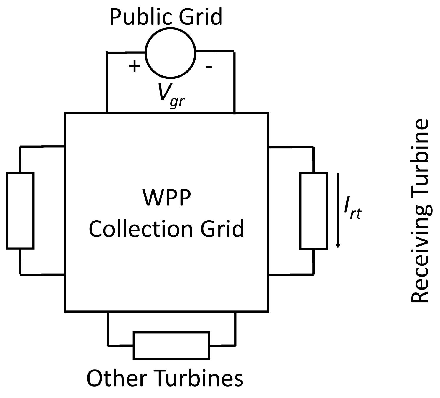
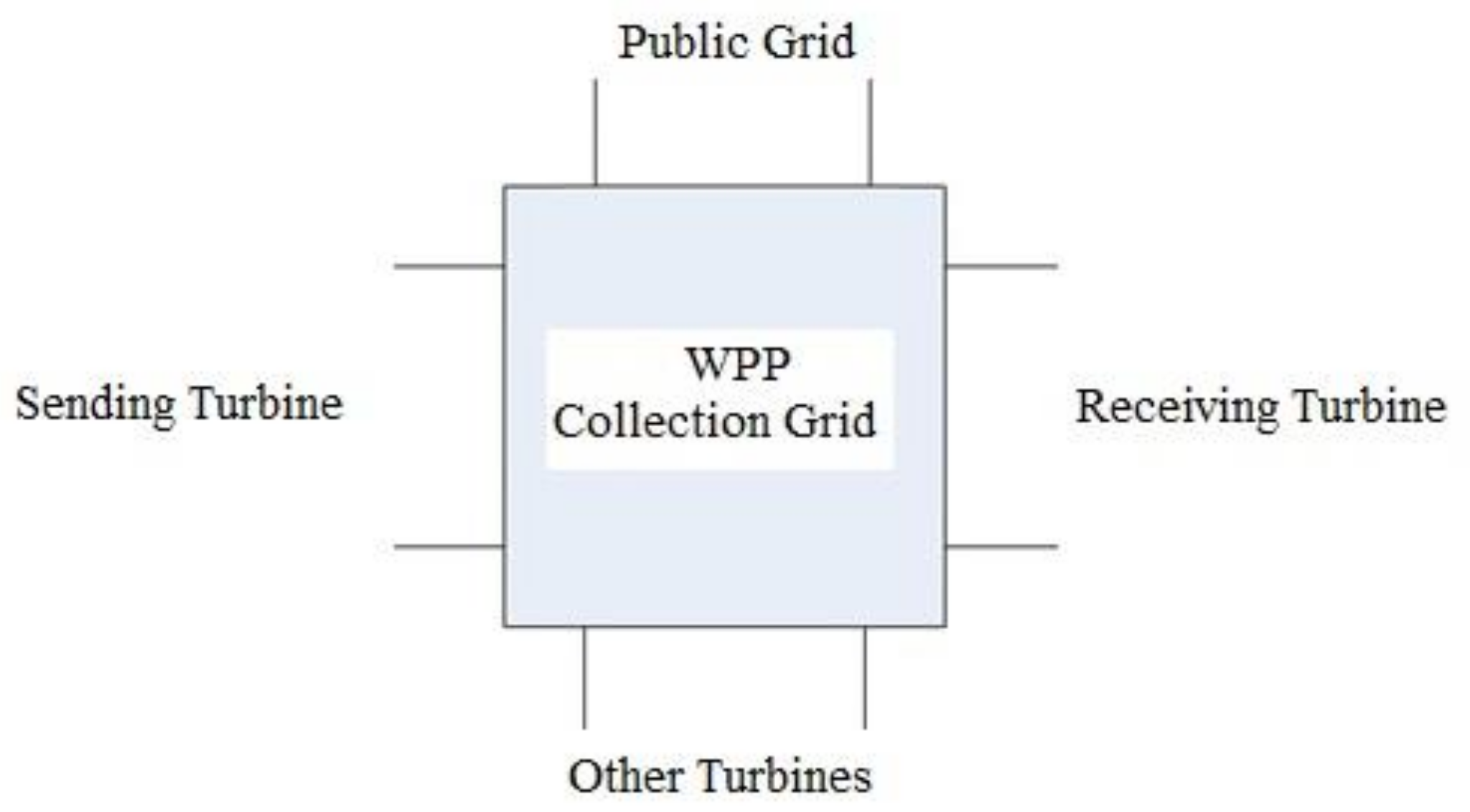
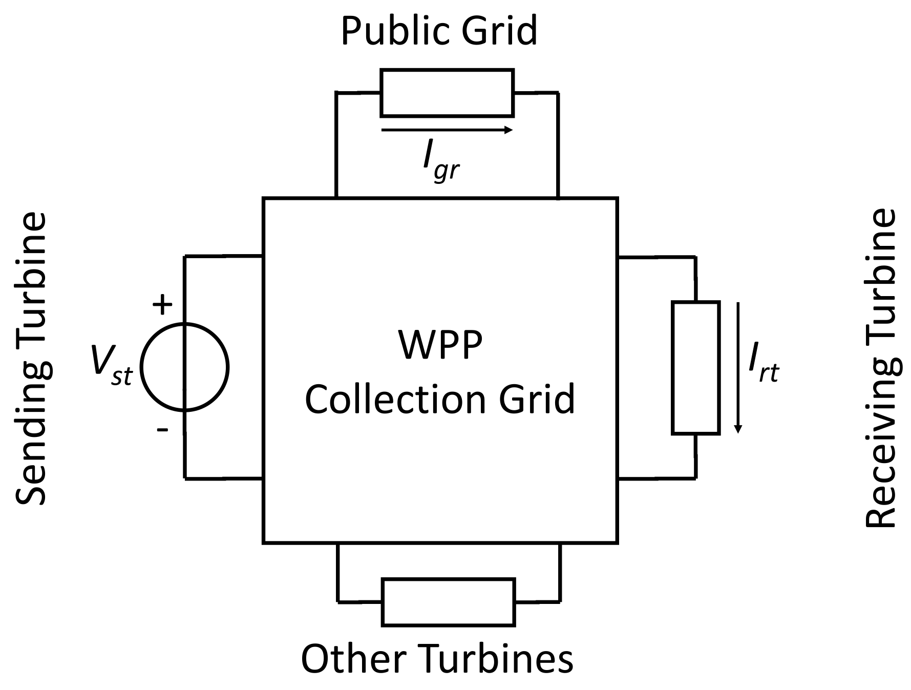
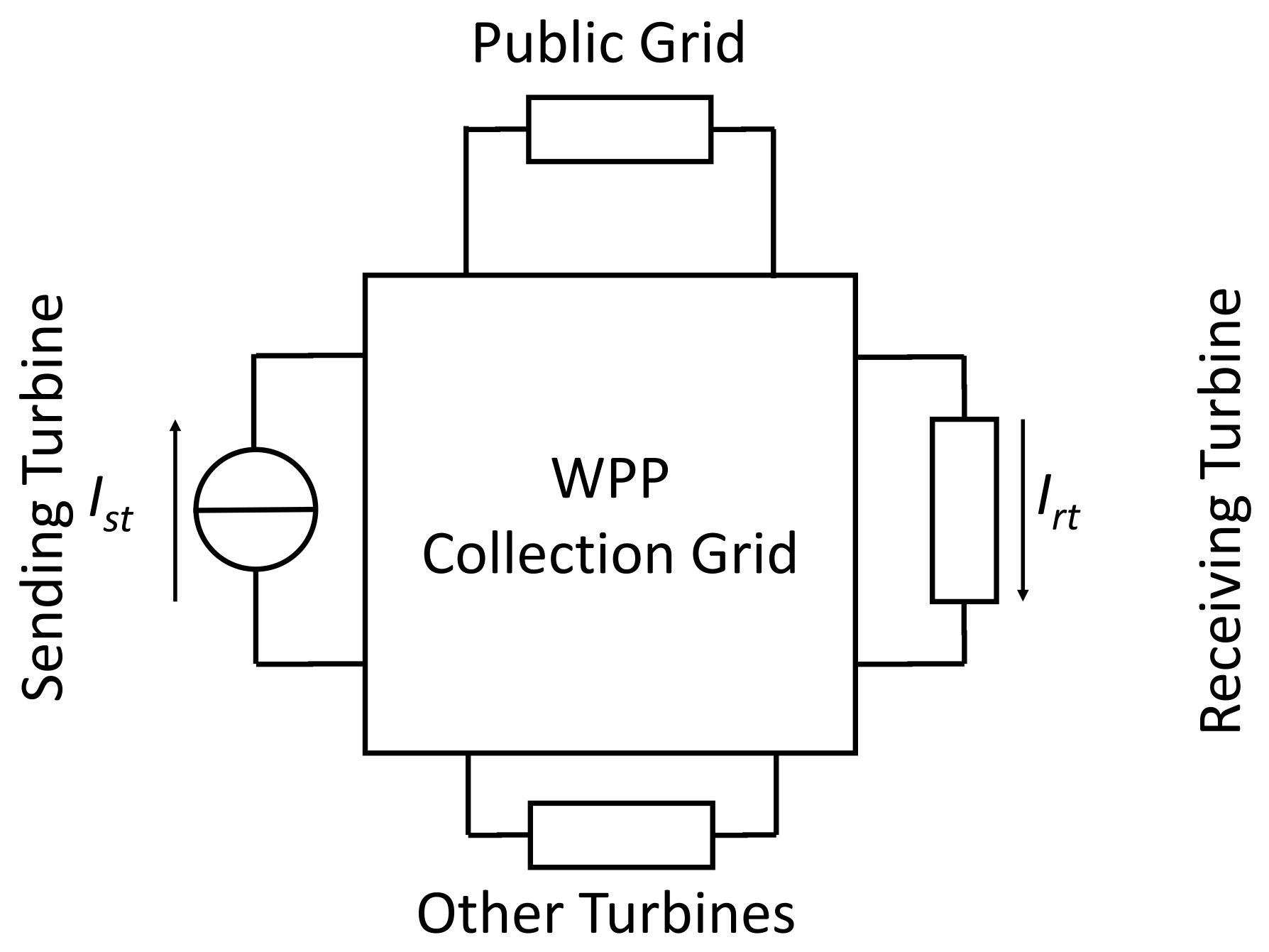
The harmonic transfers in a WPP can be quantified through a number of transfer functions: voltage transfer, current transfer, transfer admittance and transfer impedance. A multi-port circuit representation is presented in Figure 1 to illustrate how the transfers were obtained.

For the multi-port network shown in Figure 1, one sending port and one receiving port are selected. The transfer functions can be calculated for given terminations at the other ports. The sending turbine is defined as the one that is generating harmonics. The receiving turbine is defined as the one receiving the harmonics contribution. The “other turbines” in Figure 1 affect the transfer through the turbine model used, i.e., through the termination of these ports. The four transfer functions used in this paper are further explained in Appendix E.

2.2. Turbine Model

Two competing models are widely used and discussed in the literature and beyond for the harmonic emission from a wind turbine: the “voltage-source model” and the “current-source model” [22,45,46]. Neither model gives a correct representation of reality, but both models can be viewed as extreme cases. 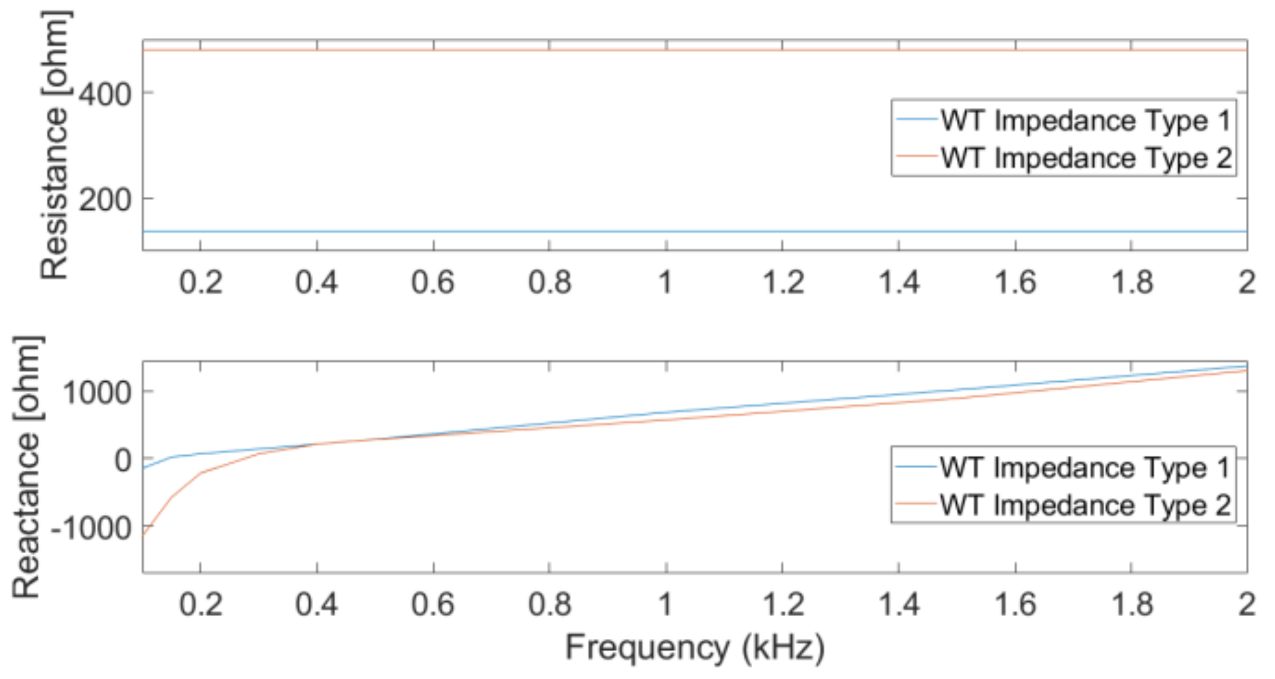Realistically modelling a voltage-source converter for harmonic studies is complicated, and a range of papers have been dedicated to this, many being trigged by [47]. Such detailed modelling is beyond the scope of this work; instead, the emphasis is on the transfers between the different converters and the grid, not on the detailed modelling of the converters. A reason for not considering detailed modelling of the converters is that such knowledge is often not available when doing studies on harmonic emission in WPPs. Sainz et al. [48] present a simplified but accurate expression for the apparent impedance of a wind turbine. For results presented in this paper, the WT impedance was obtained assuming the positive sequence results shown in ([48], Figure 4). These values include the WT converter impedance and the filters. The impedances used in this paper are shown, as a function of frequency, in Figure 2. The difference between the two types in Figure 2 is the bandwidth of the grid voltage low-pass filter $\left({\alpha }_{fv}\right)$ that was considered using Equation (2). For type 1, it was considered to be ${\alpha }_{fv,r}=1$, and for type 2, it was considered to be ${\alpha }_{fv,r}=10$. More details are found in ([48], Table 2). For this study, the impedances were calculated assuming a voltage level of 33 kV.

$${\alpha }_{fv,r}=\frac{{\alpha }_{fv}}{{\omega }_1}$$

(1)

where ${\omega }_1$ is the fundamental angular frequency.

For the calculation of the transfer function, the primary emission is modelled as an ideal voltage or current source. This does not, however, imply any assumption on which model is more representative. When calculating, for example, the transfer admittance, the primary emission for all turbines except the sending one is considered equal to zero.

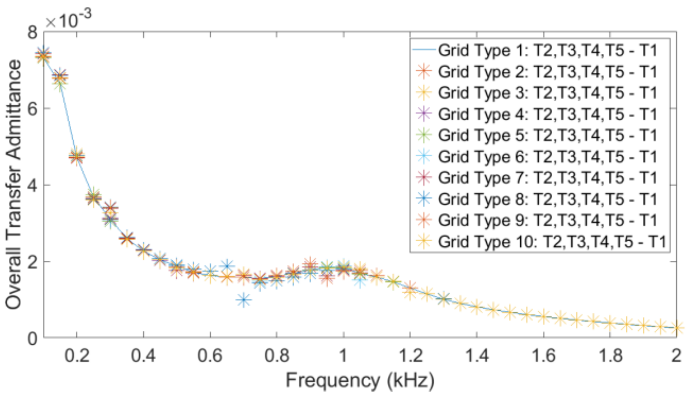
2.3. Individual and Overall Transfer Functions

An individual transfer function quantifies the transfer of harmonic voltage or current from a sending port to a receiving port, as illustrated in Figure 1. Each of these is a complex value that is a function of frequency. The transfer impedance matrix and the branch impedances were used to obtain the different transfer functions. In this paper, two transfer functions were used: the current transfer and the transfer admittance.

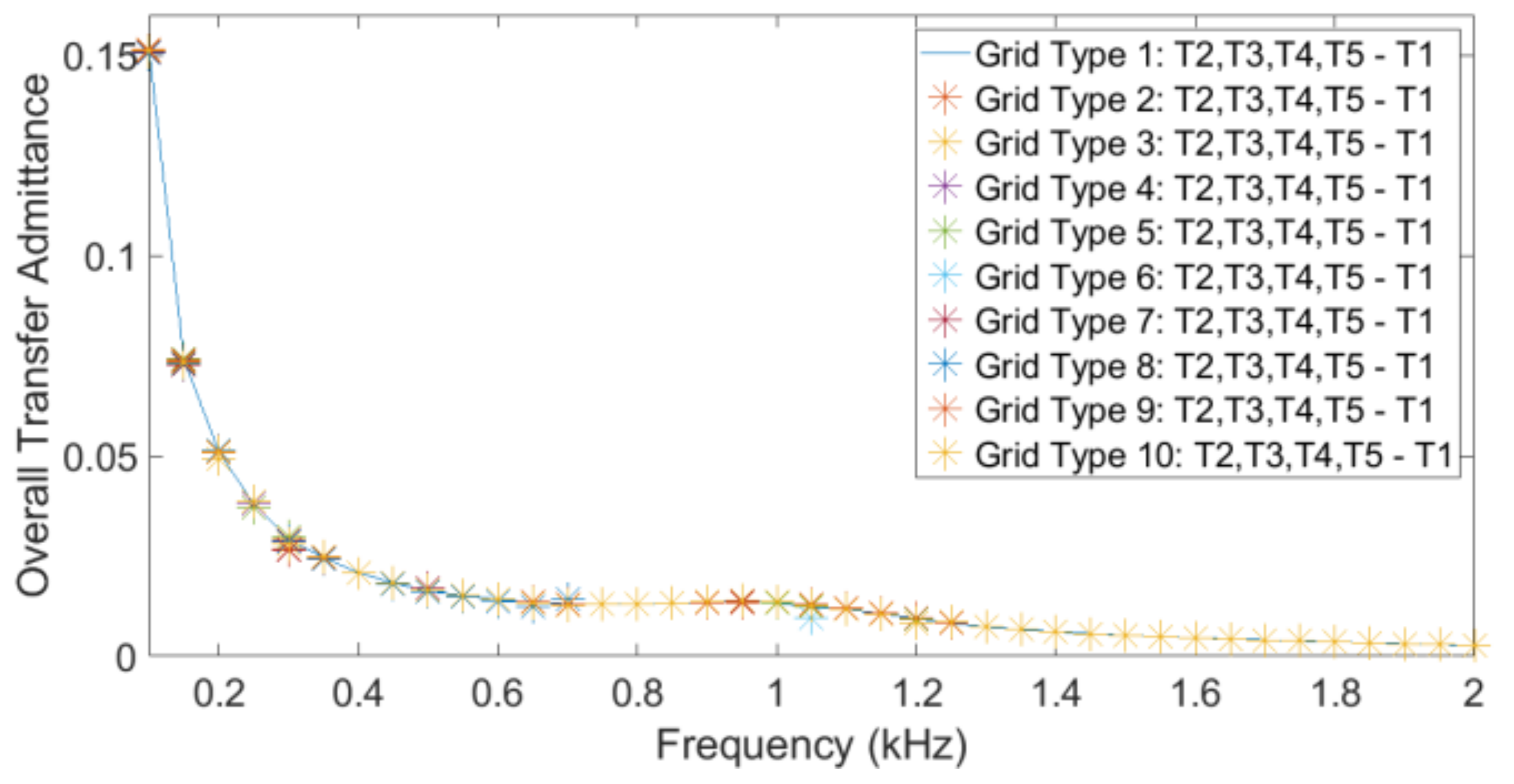
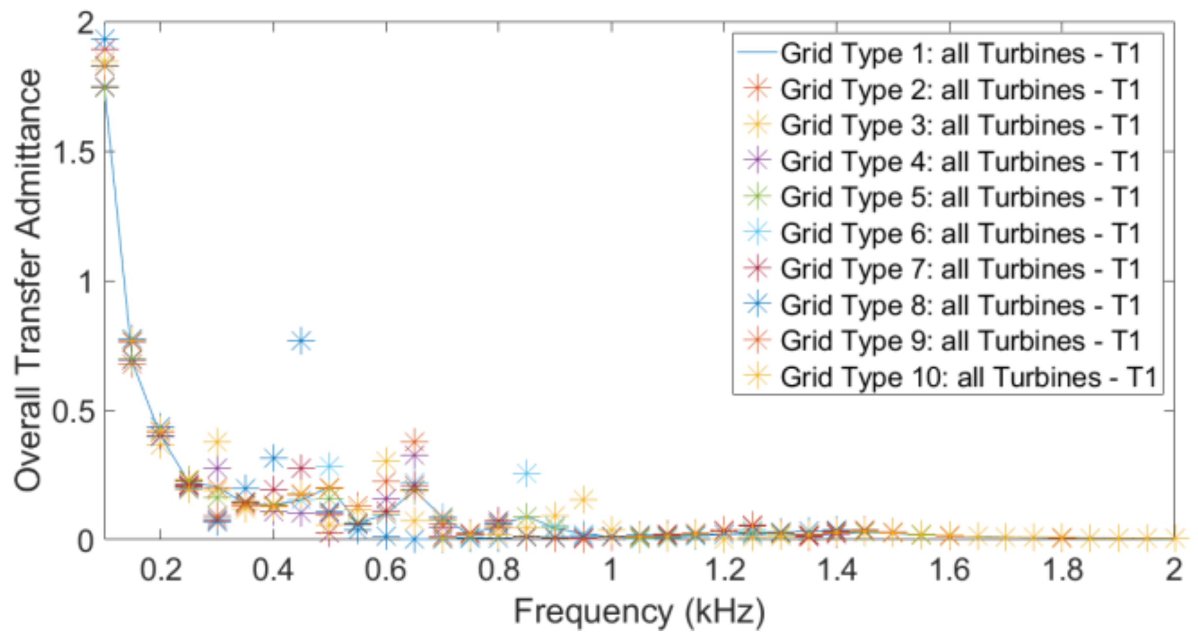
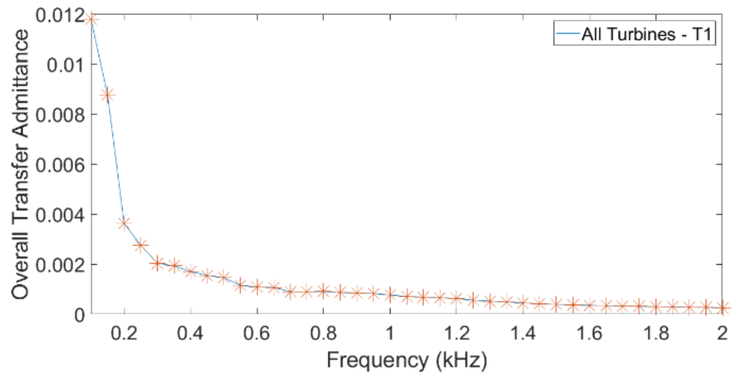
The “overall harmonic transfer” is defined as the total transfer from a number of sending ports (turbines) to one receiving port (turbine or public grid) [28,40,49].

Consider, as an example, the current transfer from turbine to public grid. The individual current transfer function is the complex ratio between the current at the public grid terminals and the current at the inverter terminals of a specific turbine, under the assumption that the emission from all other turbines is zero. The overall current transfer is defined as the ratio between grid current and turbine current when the emission is the same for all turbines. The “emission” can in this case be the absolute value of the complex current; it can also be a statistical index, such as the 95th percentile. Note that the overall transfer function is a real function of frequency, whereas the individual transfer function is a complex function of frequency.

To calculate the overall transfer from the individual transfer functions, an aggregation rule between individual turbines has to be considered. Assuming the commonly used aggregation model in IEC 61000-3-6 [14], with aggregation exponent $\alpha$, the relation between overall and individual transfers reads as Equation (2).

$$H^{\left(o\right)}=\sqrt[\alpha ]{{\displaystyle \sum }_{k=1}^N{\left(H_k^{\left(i\right)}\right)}^{\alpha }}$$

(2)

where $H^{\left(o\right)}$ is the overall transfer function, $H_k^{\left(i\right)}$ is the individual transfer function from turbine k to the public grid and N is the total number of turbines. It is the aggregation rule as defined in Equation (2) that has been used in this paper.

2.4. Calculation Method

To calculate the different individual transfer functions, the collection grid, the turbines and the public grid were all modelled as series and shunt impedances. A single-phase model was used, representing only positive- and negative-sequence harmonic components. Both transmission and turbine transformer were delta-star-connected, blocking any zero-sequence harmonic component. There was no transfer of zero-sequence components between the turbines or between turbines and the public grid.

All impedances, voltages and currents were transformed to the 33 kV voltage level of the medium-voltage collection grid. To avoid difficulties with interpretation of the results, relevant values of the transfer functions are presented in %/% on a base of rating of either the transmission transformer or the turbine transformer.

From the branch impedances, a node admittance matrix was obtained as a function of frequency. By inversion of this matrix, a node impedance matrix was obtained. This matrix was next used to calculate the different transfer functions as a function of frequency.

2.5. Case Studies

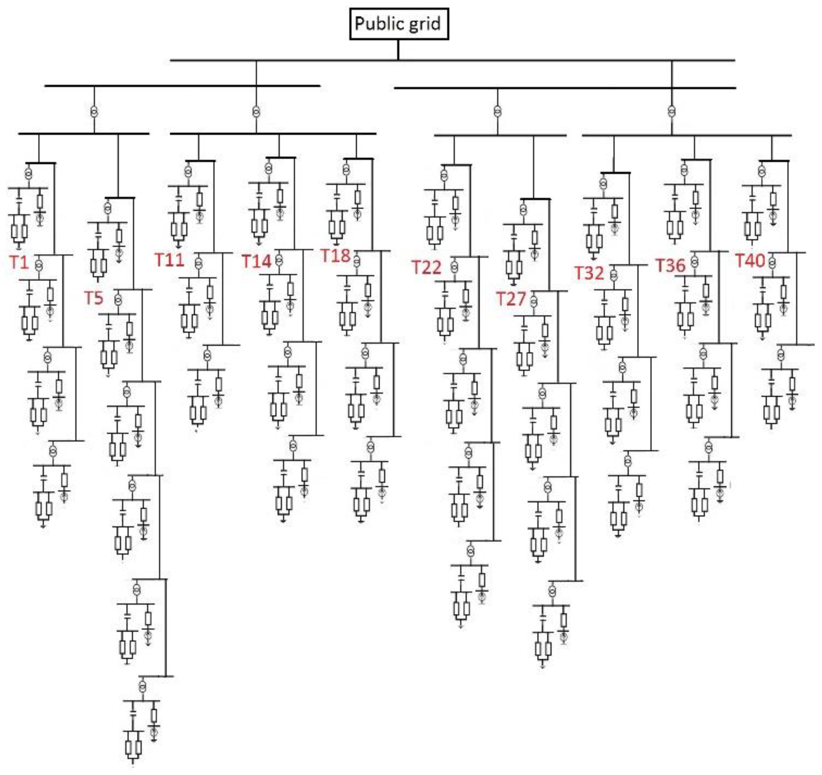
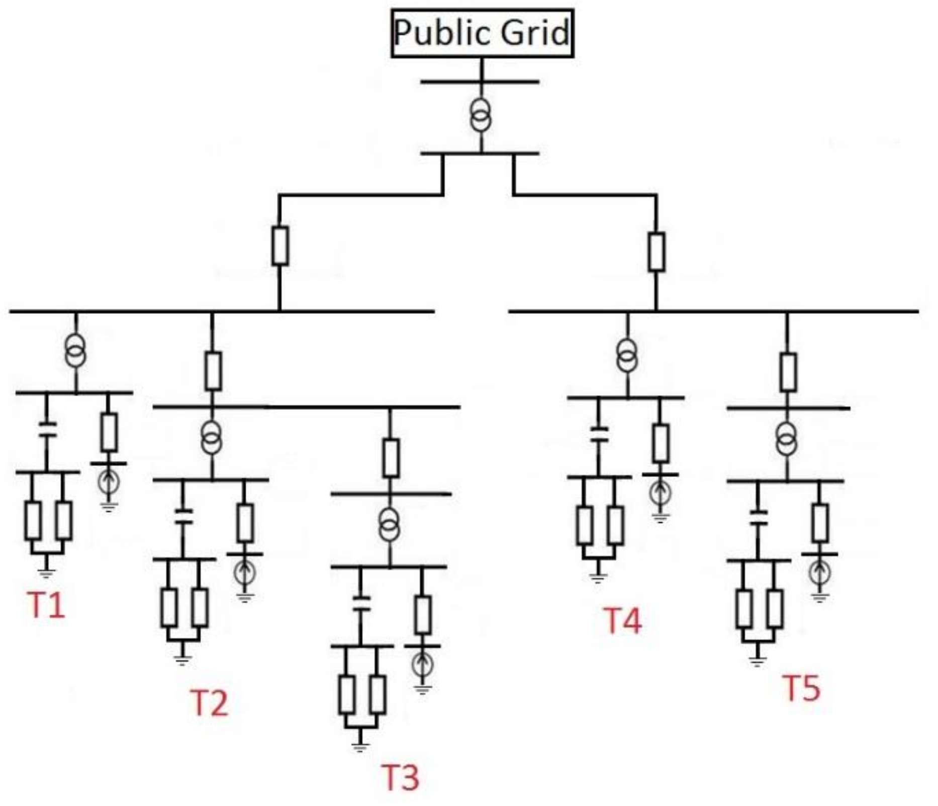
To illustrate the transfer function approach, the harmonic propagation was studied for two wind power plants, with 5 and 42 wind turbines, respectively. The details of these two WPPs are given in Appendix A and Appendix B, respectively. The 42-turbine case is an existing plant, where detailed data were obtained from the manufacturer of the installation. The 5-turbine case is a hypothetical but realistic case, where, for example, the harmonic filter selected was the same as that for the 42-turbine wind power plant.

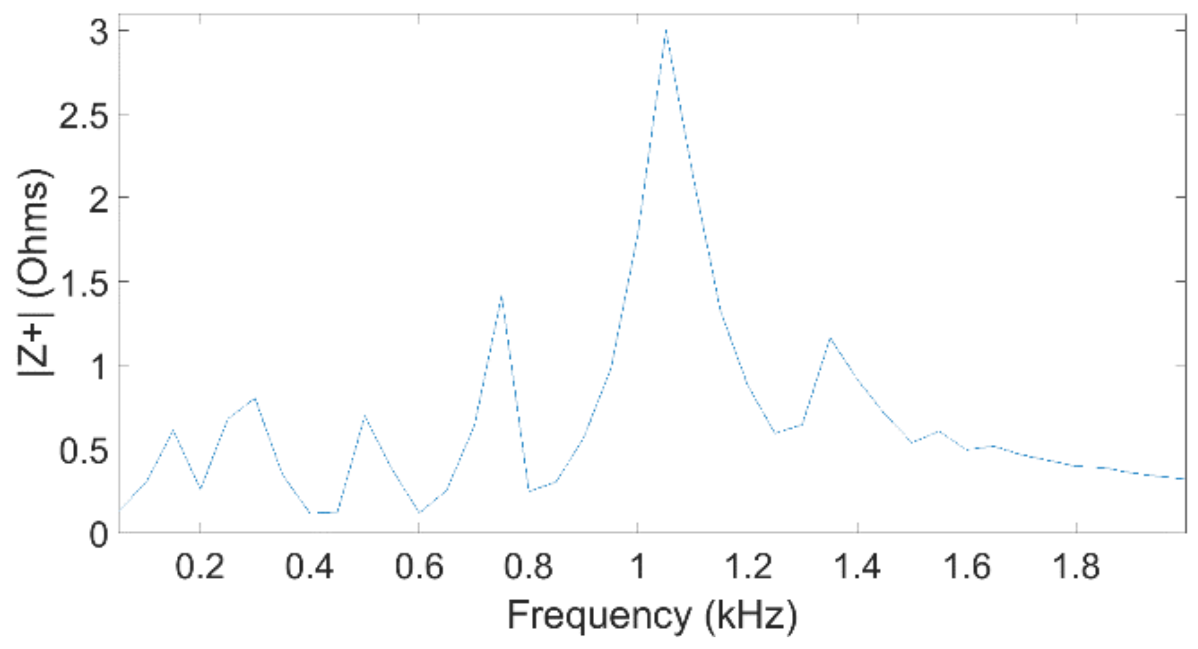
The public grid impedance versus frequency, from 100 Hz to 2 kHz, was obtained from detailed simulations of a 220-kV grid somewhere in Europe. This data are shown in Appendix C.

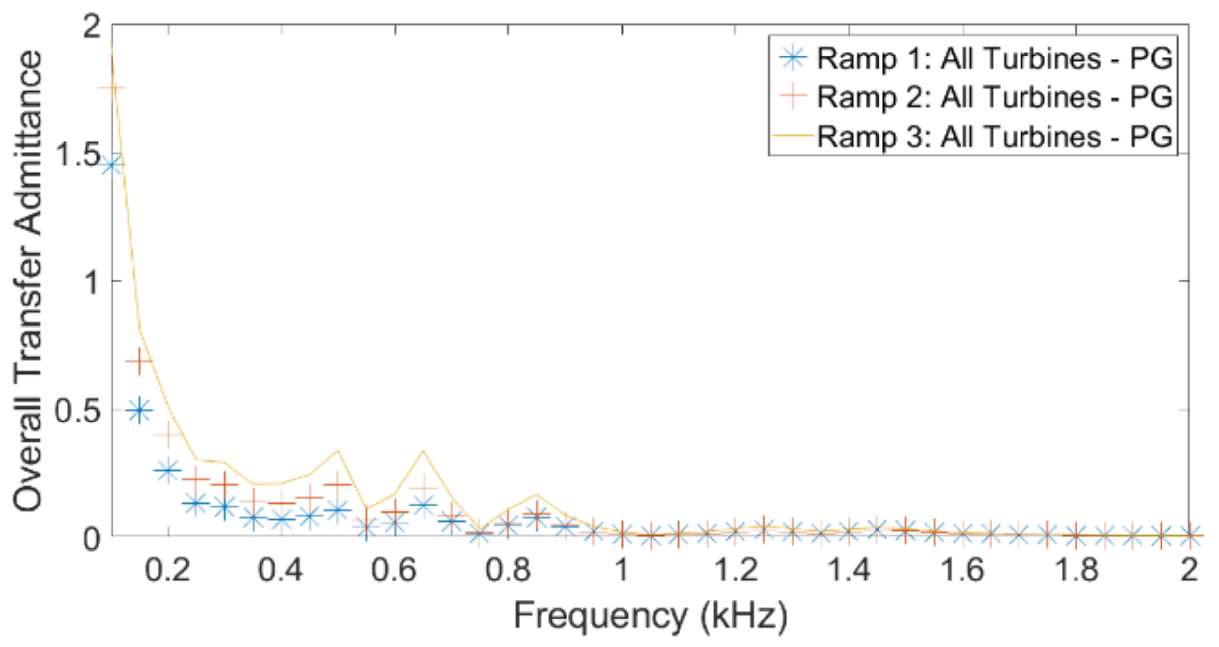
For calculation of the overall transfer functions, the aggregation exponent is needed for each frequency considered. Three models for this exponent are presented in Appendix D: next to the IEC-recommended values [14], two models with a smoother transition from exponent value 1 to exponent value 2.

2.6. The Rationale behind Transfer Functions

A transfer function gives the relation between an input variable and an output variable for a linear system. The most commonly used example, in electric power engineering, is Ohm’s law:

$$V=R\cdot I$$

(3)

where $V$ is the voltage over a resistive element (originally, a conductor) and $I$ the current through that element. The resistance $R$ is a property of the resistive element, independent of the current and the voltage. Alternatively, the ratio between voltage and current is constant, and this constant is called the resistance.

$$R=\frac{V}{I}$$

(4)

In terms of system theory, the current $I$ is the input and the voltage $V$ is the output.

For most electric circuits, the transfer functions are complex functions of frequency. Consider, for example, the parallel connection of a resistance $R$, an inductance $L$ and a capacitance $C$. Consider the voltage $V\left(\omega \right)$ as an input variable and the current $I\left(\omega \right)$ as an output variable. The ratio between current and voltage, the admittance, reads, for this example, as

$$Y\left(\omega \right)=\frac{I\left(\omega \right)}{V\left(\omega \right)}=R+j\omega C+\frac{1}{j\omega L}$$

(5)

where $\omega =2\pi \cdot f$ is the angular speed and $f$ is the frequency. The admittance, a transfer function, is a function of frequency, but that function is independent of the actual voltage and current at any frequency.

In the examples up to now, the input and output variables have been taken at the same location in the electric circuit. In that case, we often refer to the transfer function as source or driving-point impedance or admittance. The term “transfer impedance” or “admittance” (or generally, transfer function), however, also holds for this case.

In a power grid with many elements, like the combination of a WPP and the grid studied in this paper, the calculation of the transfer functions is no longer as straightforward as in the two examples shown here. Instead, more systematic methods are used, which can be implemented in calculation software. Several software packages have the ability to perform such calculations, all using somewhat different methods. In this paper, we used the following approach:

➢

The complex impedances of each branch in the network were given; from these branch impedances, the branch admittances were calculated through a simple arithmetic inversion. These branches included cables (modelled as a pi-model including series resistance, series inductance and shunt capacitance), transformers, grid impedance and turbine impedance.

➢

The so-called node admittance matrix was obtained by adding the branch admittances one by one.

➢

The node impedance matrix was calculated through a matrix inversion of the node admittance matrix.

The node impedance matrix was used for the calculation of the transfer functions. Each of the branches has an impact on the elements in the node impedance matrix and thus on the transfer functions. It is, however, in most cases, not possible to identify the impact of a specific branch impedance on a specific transfer function. The combination of all branches in the network matters for the transfer function.

For a linear system with multiple inputs, the superposition principle can be used to obtain the output. A relevant example for this paper is the case with multiple turbines emitting harmonic currents that all contribute to the harmonic voltage at a specific location in the park. The voltage $U_r\left(\omega \right)$ at a location r is obtained from the following expression:

$$U_r\left(\omega \right)={\displaystyle \sum }_{s=1}^N{Z}_{rs}\left(\omega \right)\cdot I_s\left(\omega \right)$$

(6)

where $Z_{rs}\left(\omega \right)$ is the transfer impedance from location s to location r and $I_s\left(\omega \right)$ the injected current at location s. Note again that voltage, current and transfer impedance are complex functions of frequency.

3. Results

The harmonic transfer functions described in Section 2 were calculated for the two WPPs defined in Appendix A and Appendix B. The harmonic transfers between turbines, into the collection grid and into the public grid, were obtained, and some of the results are presented in the forthcoming subsections.

3.1. Transfer from Turbine to Public Grid

The overall transfer admittance was calculated for both WPPs. The results are presented in Figure 3 and Figure 4 for the 5-turbine and 42-turbine plants, respectively.

When considering the individual transfer admittance, the sending node (one turbine) was modelled as a voltage source and the receiving node (public grid) through the impedance versus frequency shown in Figure A3 (Appendix C). To obtain the overall transfer admittance, the contribution of all these transfers was included, using Equation (2) and the aggregation exponents according to IEC 61000-3-6 [14], as shown in

Table A6. Aggregation exponent for harmonic studies.

Harmonic Order	α According to IEC 61000-3-6
h > 5	1
5 ≤ h ≤ 10	1.4
10 > h	2
Harmonic Order	α According to Ramp 1
h ≤ 10	$1+\left[\left(\mathrm{h}-1\right)\times 0.1111\right]$
h ≥ 10	2
Harmonic Order	α According to Ramp 2
h ≤ 19	$1+\left[\left(\mathrm{h}-1\right)\times 0.0526\right]$
h ≥ 20	2
Harmonic Order	α According to Ramp 3
h ≤ 19	$1+\left[\left(\mathrm{h}-1\right)\times 0.0256\right]$
h ≥ 20	2

in Appendix D. As, for both cases, the individual transfer functions are similar, independent of the considered turbine, only the results for the overall transfer function are presented. For the five-turbine case, for the frequencies 100 Hz and 1 kHz, the admittances were 0.1513 A/V and 0.01327 A/V, respectively, as presented in Figure 3.

To enable easier interpretation, per unit values were again used. Using the rating of the public grid transformer (30 MVA) as a base, 1 p.u. voltage distortion with the turbine have 5.49 p.u. (at 100 Hz) and 0.48 p.u. (at 1 kHz) harmonic current flowing into the public grid.

For the 42-turbine case, Figure 4 presents the results. In this case, for the same frequencies, the admittances were 1.747 A/V and 0.01107 A/V, giving 17.29 p.u. (at 100 Hz) and 0.11 p.u. (at 1 kHz) of current distortion for 1 p.u. of voltage distortion, using a power base equal to the public grid transformer rating (110 MVA).

3.2. Transfer from Turbine to Turbine

The overall transfer admittance (voltage to current) and the overall current transfer (current to current) were calculated for both WPPs. The results are presented in Figure 5, Figure 6, Figure 7 and Figure 8. Note the small values along the vertical scale in Figure 5.

To calculate the individual transfer functions, the sending port (one turbine) was modelled as a voltage source, all other turbines through their representative impedance (see Section 2.2 and Appendix E) and the public grid through the impedance shown in Figure A3 (Appendix C). Figure 6 and Figure 7 present the overall transfer admittance results. In Figure 5, for 100 Hz and 1 kHz, the overall transfer was 0.0072 V/A and 0.00181 V/A, respectively, for the five-turbine case. Considering the 42-turbine case, from Figure 6, the values were 0.0118 V/A and 0.0007672 V/A, respectively. Considering the wind power plant with five turbines, assuming the rated power of the WT transformer as the power base, 1 p.u. voltage distortion for each turbine gave 0.33 p.u. current distortion at the receiving turbine. For the 42-turbine case, 1 p.u. voltage distortion gave 1.98 p.u. (at 100 Hz) and 0.13 p.u. (at 1 kHz) for current distortion, as presented in Figure 6.

The overall transfer to a given turbine was calculated by combining the individual transfers from the four other turbines to the given turbine. In Figure 7, the overall current transfer function for the five-turbine case is presented. At 100 Hz and 1 kHz, the transfer was 0.26 A/A and 0.62 A/A, respectively. For the 42-turbine case, Figure 8, the values were 0.3 A/A and 0.28 A/A, respectively, meaning that the total secondary emission, driven by all the other turbines together, was 30% and 28%, respectively, of the primary emission. This is a significant amount, which cannot be neglected. Note again that neither primary nor secondary emission can be quantified using only transfer functions; it is, however, possible to quantify the ratio between primary and secondary emissions.

3.3. Transfer from Grid to Turbine

Considering the transfer from the public grid to the turbines, the transfer admittance was calculated for both WPPs. The results are presented in Figure 9 and Figure 10.

Considering the individual transfer admittance, the sending port (public grid) was modelled as a voltage source behind the impedance defined in Figure A3 (Appendix C) and the receiving port (one of the turbines) as well as all other turbines through their equivalent impedance. In Figure 9, for the five-turbine case, the admittance for 100 Hz and 1 kHz was 0.007006 V/A and 0.005247 V/A, respectively. Assuming the rated current of the WT transformer, 1 p.u. voltage distortion (primary emission) gave 1.27 p.u. and 0.95 p.u. current distortion (secondary emission) for the turbines. For the 42-turbine case (Figure 10), the transfer admittance at 100 Hz and 1 kHz was 0.006954 V/A and 0.006147 V/A, respectively. Considering 1 p.u. voltage distortion, this corresponds to 1.16 p.u. and 0.1 p.u. current distortion for each of the turbines.

3.4. Impact of Aggregation Model

Due to variations in wind speed and due to variations in emission even for the same wind speed, the harmonic emission from a wind turbine is time-varying in magnitude [39] and in phase angle [49]. The primary harmonic emission of the WPP is the summation of all contributions from the individual wind turbines. As harmonic currents and voltages can be represented by vectors, both magnitude and phase angle of the individual vectors are needed. The summation law in IEC 61000-3-6 [14] can be used to determine the total harmonic contribution of a WPP. Depending on the harmonic order, different aggregation behaviours are noticed [40], so different aggregation exponents should be considered.

An aggregation exponent is also included in the overall transfer function calculation. However, as shown in [31], the aggregation exponent is not only dependent on the harmonic order but also is different for different types of wind turbines. To study the impact of this, four aggregation exponent profiles were considered. The resulting overall current and voltage transfers were compared, as presented in Figure 11 and Figure 12. The used values for the aggregation exponent, referred to as “Ramp 1”, “Ramp 2”, and “Ramp 3”, are presented in Table A6 in Appendix D.

Considering the 42-turbine case, the overall harmonic current transfer and transfer admittance are presented in Figure 11 and Figure 12, respectively. Both figures show that the used aggregation exponent plays an important role in the overall transfer. It is important to consider aggregation when calculating the total contribution of the WPP. As an example, in

Table 1. Summary of the different transfer functions for selected harmonic orders.

Overall transfer admittance from turbine to grid
Harmonic Order	Ramp 1	Ramp 2	Ramp 3
Harmonic 3	0.49 V/A	0.68 V/A	0.81 V/A
Harmonic 17	0.08 V/A	0.09 V/A	0.17 V/A
Overall current transfer from turbine to grid
Harmonic Order	Ramp 1	Ramp 2	Ramp 3
Harmonic 3	18.06 A/A	25 A/A	30 A/A
Harmonic 17	23 A/A	26.5 A/A	49.33 A/A

, a comparison of the obtained results for the transfer current and transfer admittance is presented considering harmonics 3 and 17.

3.5. Impact of Turbine Impedance

3.5.1. Transfer from Turbine to Turbine

The secondary emission between turbines, for different WT harmonic impedances, is presented for both WPPs in Figure 13 and Figure 14. Note the small values along the vertical scale of Figure 13.

Figure 13 shows a significant difference when different harmonic impedances are assumed for the WT. As type 2 has higher impedance, the secondary emission was lower for low-order harmonics. However, for high-order harmonics, both impedances showed a similar behaviour for the secondary emission. For 100 Hz, considering type 1, the transfer was about 0.0072 A/V; for 1 kHz, the transfer was about 0.0018 A/V. For type 2, the transfer was about 0.0010 A/V for 100 Hz and about 0.0013 A/V for 1 kHz.

For the second case, with 42 turbines, presented in Figure 14, the same conclusion was found for low-order harmonics as in the previous case. For high-order harmonics, there is a small difference between the overall transfer admittance for the two WT impedances. This holds especially from 1.4 kHz. Considering type 1, for 100 Hz, the transfer was 0.0118 A/V; for 1 kHz, it was 0.0007672 A/V. Assuming type 2, the transfer was 0.001681 A/V for 100 Hz and 0.00006346 A/V for 1 kHz.

3.5.2. Transfer from Turbine to Public Grid

The transfer emission from turbine to public grid, for different WT harmonic impedances, is shown in Figure 15 and Figure 16.

The WT impedance had a lower impact on the transfer from the turbines to the public grid for high-order harmonics than for low-order harmonics. For low-order harmonics, the impact was not as big as for the transfer between turbines. From Figure 15, assuming WT impedance type 1, the transfer was 0.1513 A/V for 100 Hz and 0.0138 A/V for 1 kHz. For type 2, the transfer was 0.1413 A/V and 0.0098 A/V for 100 Hz and 1 kHz, respectively.

For the 42-turbine case, presented in Figure 16, for low-order harmonics, the same conclusion was found as for the 5-turbine case. Considering type 1, the transfer was 1.747 A/V for 100 Hz and 0.01107 A/V for 1 kHz. Assuming type 2, the transfer was 1.632 A/V for 100 Hz and 0.009785 A/V for 1 kHz. The transfer admittance from turbine to public grid matters for the primary emission of the WPP into the public grid. Uncertainties in this transfer admittance result in uncertainties in the primary emission of the WPP, even when the primary emission of the turbines is known.

3.5.3. Quantifying the Impact

Transfer functions can be used to estimate the harmonic contribution within a WPP, towards the public grid or any other location. Based on this, in this paper, a sensitivity analysis was performed to estimate the impact of the WT impedance and the public grid impedance on the harmonic transfers between turbines and towards the public grid. A comparison of the presented results in the previous section was used to quantify their impact on the different transfer functions and thus on primary and secondary emissions.

To quantify the impact of the WT impedance (type 1 or type 2) on the transfer admittance, the relative difference according to Equation (3) is presented in Figure 17 and Figure 18.

$$\Delta Y=\left|\frac{Y_{Type1}-Y_{Type2}}{Y_{Type1}}\right|\times 100\%$$

(7)

From Figure 17, one can observe how important it is to use the proper model of the WT impedance for quantifying transfer between turbines and thus for quantifying the secondary emission. The differences were similar for the two WPPs, with a high difference occurring for low-order harmonics (over 80% at 100 Hz) and around the resonant frequency (20–30%).

Figure 18 shows that the impact of the WT impedance was less for the transfer to the grid than for the transfer between turbines at low-order harmonics (30–60%). Around the resonant frequency, the impact was similar (30–40%). The impact was, also here, similar for the two WPPs, with the exception of a big difference for the 42-turbine case at 150 Hz (0.15 kHz).

Figure 18 shows that the impedance of the turbines also affected the primary emission from the WPP to the public grid. Lack of knowledge of the turbine impedance does result in an uncertainty of the primary emission of the WPP.

3.6. Impact of Public Grid Impedance

3.6.1. Transfer from Turbine to Turbine

The transfer admittance from turbine to turbine, for different grid impedances, is presented for both WPPs in Figure 19 and Figure 20. This transfer is an important contribution to the secondary emission between turbines.

From Figure 19 and Figure 20, one can observe that the public grid impedance affected the transfer between turbines only for lower-order harmonics: up to 1.2 kHz and 0.65 kHz, for the 5-turbine and 42-turbine cases, respectively. For those lower-order harmonics, the transfer was affected mainly around frequencies with high public grid impedance, associated with resonances in the public grid. For higher frequencies, the different scenarios had little impact on the transfer between the turbines.

3.6.2. Transfer from Turbine to Public Grid

The primary emission from the turbines to the public grid, for different public grid impedances, is presented for both plants in Figure 21 and Figure 22.

Figure 21 and Figure 22 show the big difference in the impact of the public grid impedance on the two WPPs. For the 5-turbine plant, the impact was much smaller than for the 42-turbine plant.

Considering the five-turbine wind power plant, presented in Figure 21, at frequency 100 Hz, the highest transfer was 0.1514 A/V and the lowest 0.1506 A/V. At frequency 1 kHz, the highest transfer was 0.01362 A/V and the lowest 0.01321 A/V. In the 42-turbine case, Figure 22, the highest and lowest values for 100 Hz were 1.93 A/V and 1.746 A/V, respectively. For 1 kHz, these values were 0.0379 A/V and 0.008926 A/V, respectively.

3.6.3. Quantifying the Impact

In the same way as in Section 3.5.3, the impact of the public grid impedance is shown as a percentage difference in Figure 23 and Figure 24.

From Figure 23, one can observe that it is equally important to use the correct model for the public grid impedance when studying the secondary emission. The difference is generally small (up to about 15%), but for specific harmonic orders, the difference is much higher (40–50%). The harmonic orders at which this occurs were different for the two plants.

Considering the primary emission from the turbines to the public grid (Figure 24), one could observe a big difference in impact between the 42-turbine case and the 5-turbine case. For the latter, the impact was small, up to 20%, but below 10% for most frequencies. For the 42-turbine case, the impact was much bigger for this transfer than for the transfer between turbines. Big differences (80–100%) were observed in the frequency range from 0.3 kHz to 1.4 kHz.

4. Discussion

In this paper, primary and secondary emissions of a wind power plant were studied by using different transfer functions. It was shown that the transfer functions are a suitable tool for this. The transfer functions were calculated for two cases: (i) a hypothetical WPP with 5 wind turbines and (ii) an existing offshore wind power plant with 42 turbines.

4.1. Primary and Secondary Emissions

The studies presented in this paper were triggered by the need to estimate the relative contribution of the secondary emission without knowing the details of the primary emission. This relative contribution was shown in the paper both for the terminals of the turbines and for the WPP terminals. The results from the different simulations are summarized, for both WPPs, in

Table 2. Different transfer functions expressed in percentage of rated voltage or current.

	5-WT WPP	42-WT WPP
Overall transfer admittance from turbine to grid
Harmonic 2	5.49%/%	17.29%/%
Harmonic 13	0.49%/%	1.89%/%
Overall transfer admittance from turbine to turbine
Harmonic 2	1.31%/%	1.98%/%
Harmonic 13	0.28%/%	0.18%/%
Overall current transfer from turbine to turbine
Harmonic 2	0.26%/%	0.30%/%
Harmonic 13	0.47%/%	0.21%/%
Individual transfer admittance from grid to turbine
Harmonic 2	1.27%/%	1.17%/%
Harmonic 13	0.90%/%	1.01%/%

. The values in the table give an indication of the relative magnitude of the primary and secondary emissions, where harmonic orders 2 and 13 were selected somewhat arbitrarily. The current transfer from turbine to turbine showed that the overall secondary emission, due to neighbouring turbines, is a substantial part of the primary emission. Every percentage primary emission gave between 0.33% and 1.07% secondary emission.

A direct comparison is not possible between secondary emission coming from the grid and primary emission from a turbine. Assume that voltage distortion in the grid is of the order of 1% of nominal voltage (a typical value) and that the primary emission of a turbine is of the order of 1% of rated current (a typical value). The table shows, in that case, that both contributions (primary emission from the turbines and secondary emission originating from the grid) are of the same order of magnitude.

The overall conclusion from the table is that primary emission, secondary emission from other turbines and secondary emission from the public grid are of the same order of magnitude at the turbine terminals. It will thus be difficult to estimate the magnitude of the primary emission from measurements only.

The used aggregation exponent has a strong impact on the emission when emission from multiple turbines is considered. This is the case not only around the resonant frequency but also for other frequencies. No proper aggregation model exists for use in WPPs, so further work is needed here.

Further work needed also includes applying the method to other WPPs to evaluate whether the values in Table 2 are generally representative or only hold for the two studied cases.

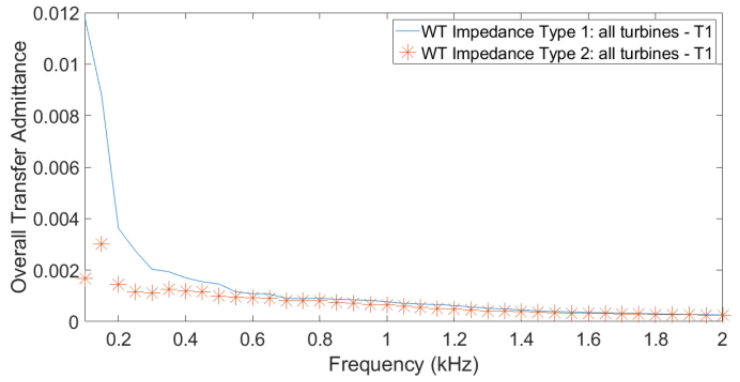
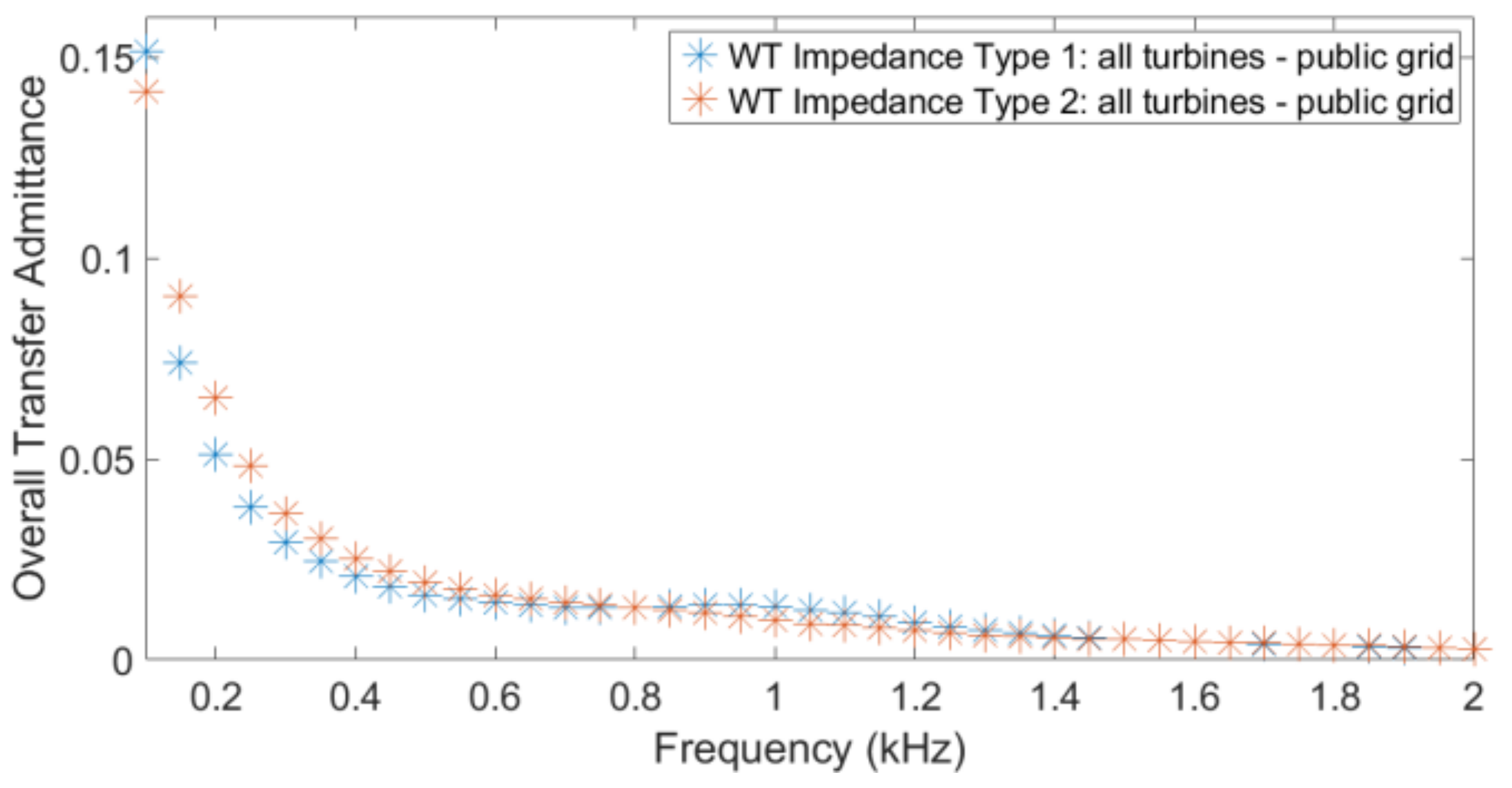
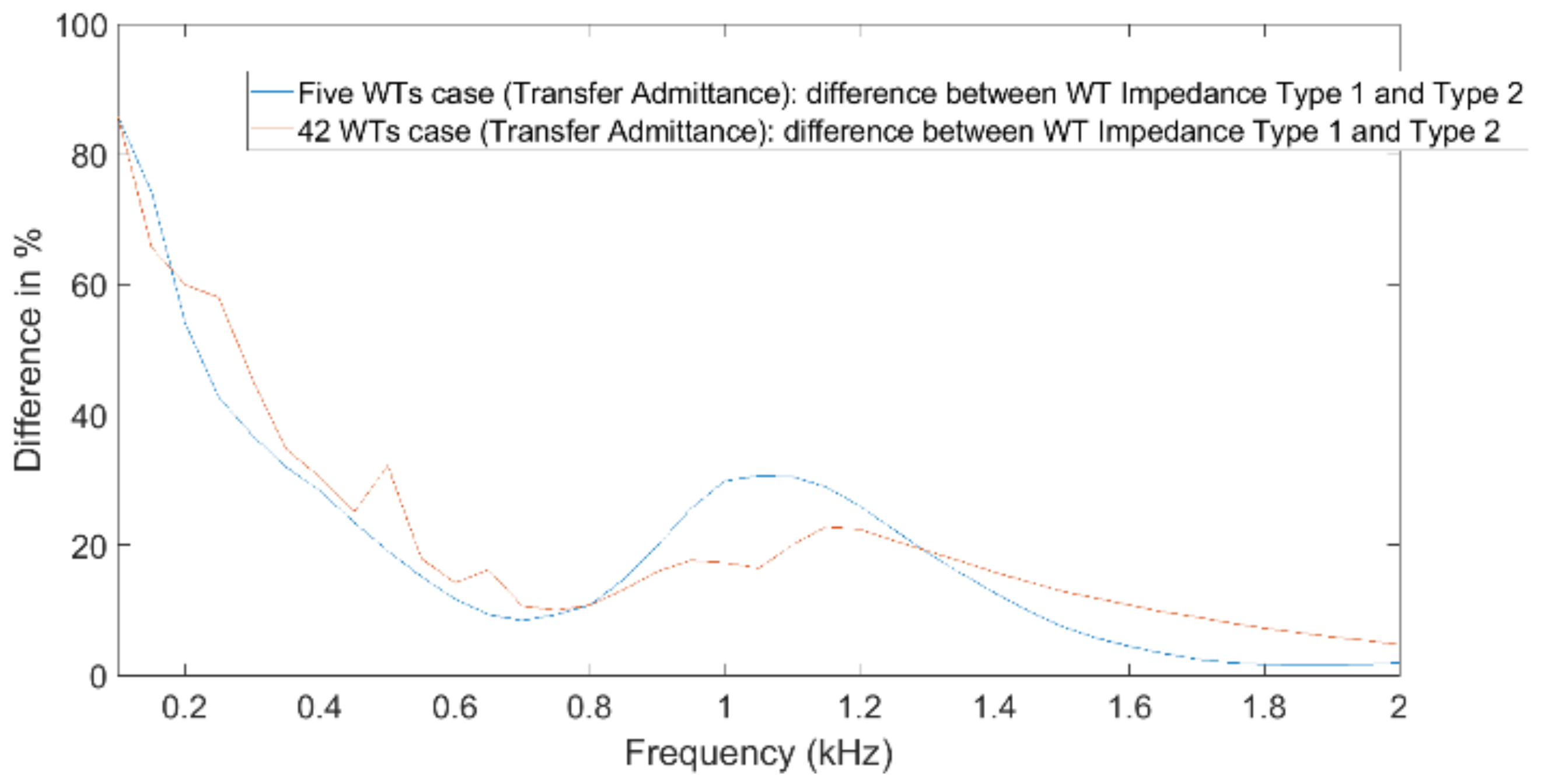
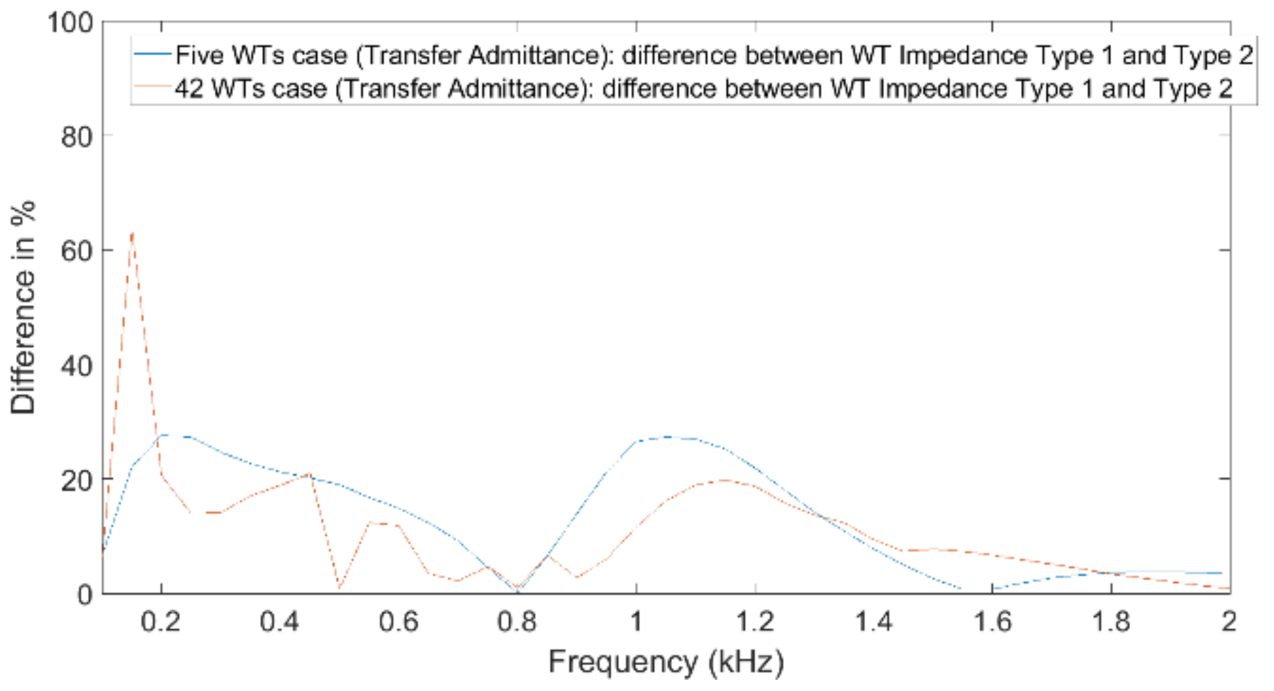
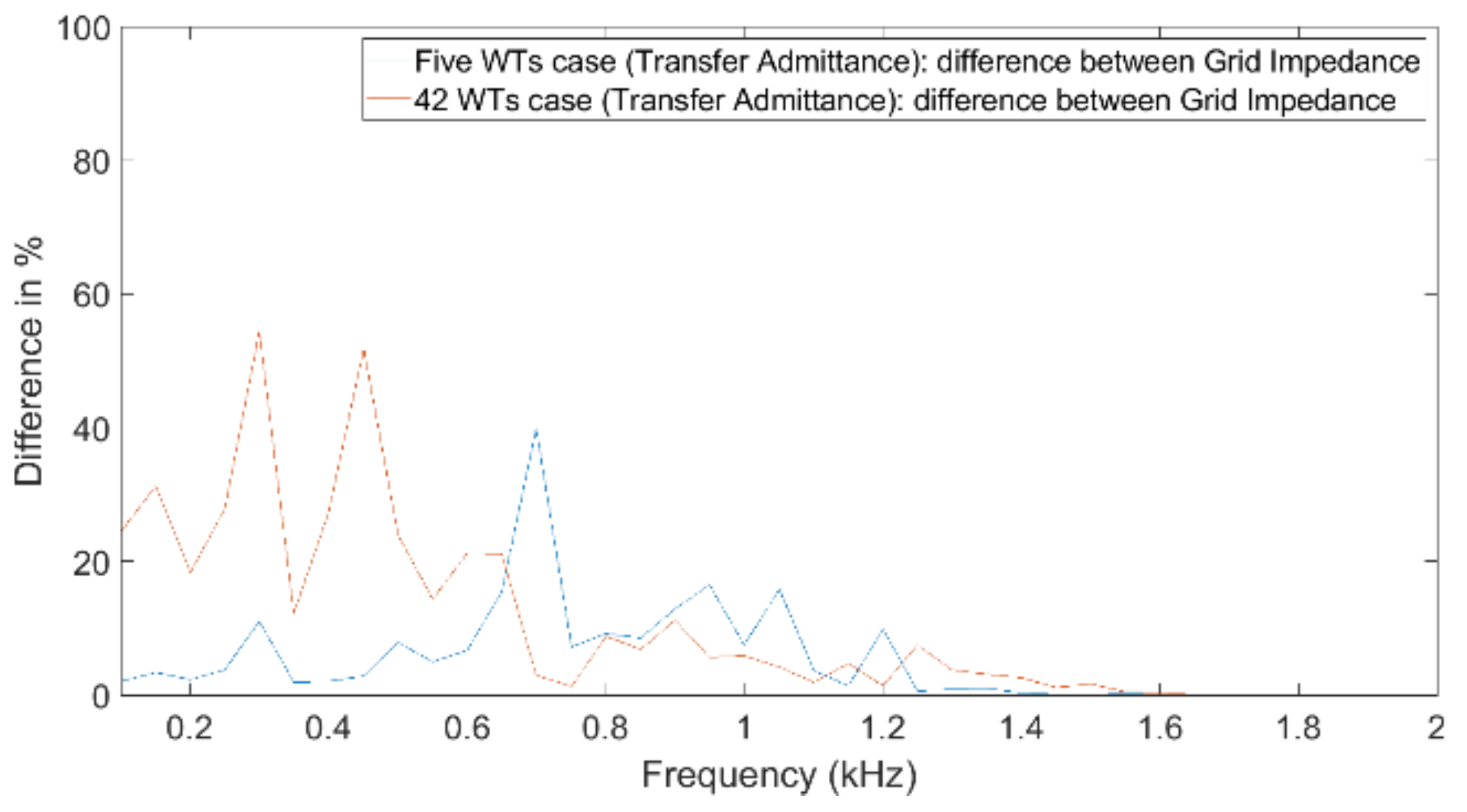
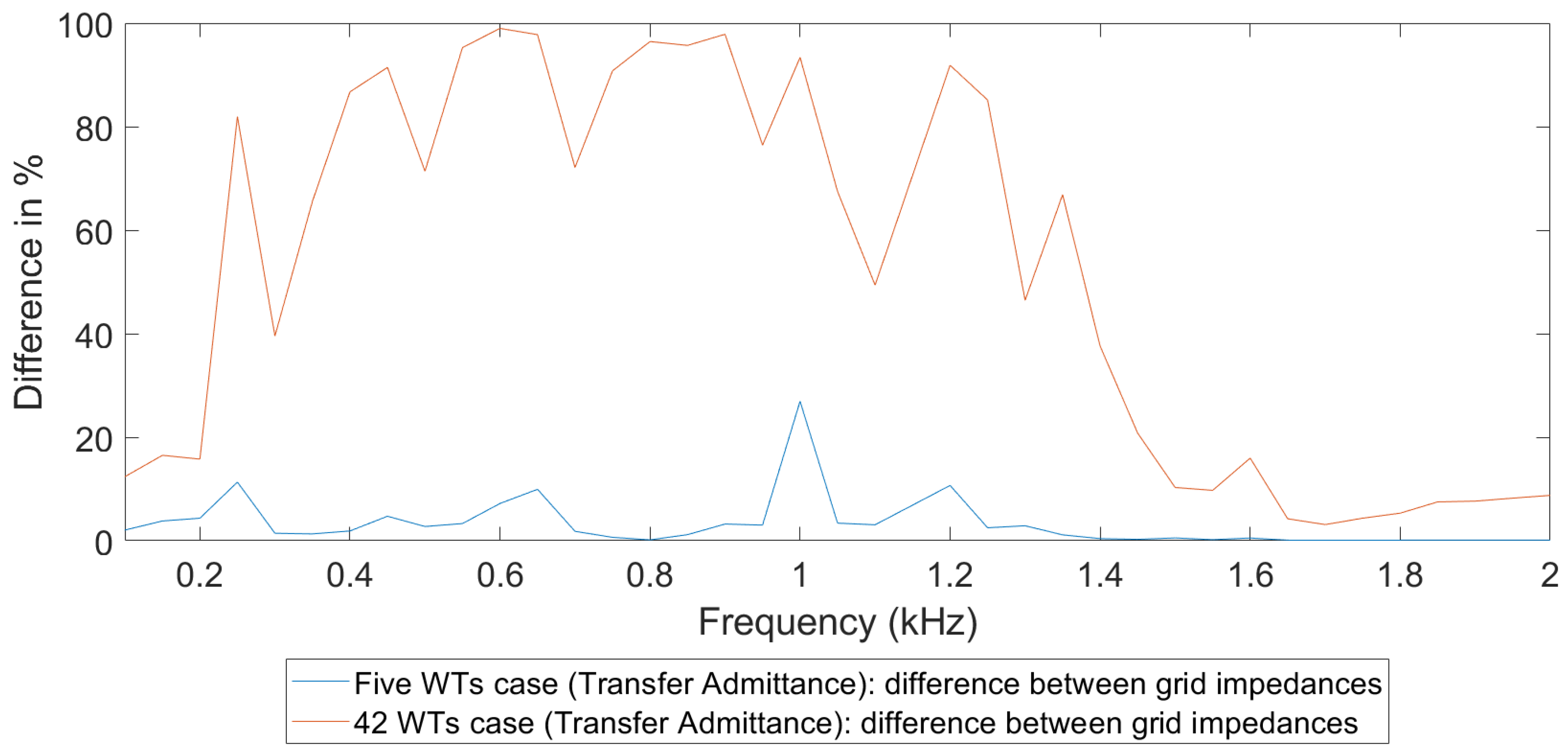
4.2. Impact of Turbine and Public Grid Impedances

In this paper, the impact on the WT impedance and the public grid impedance for harmonic studies considering WPPs is presented. Both impedances are shown to be an important factor to be considered with harmonic studies for WPPs. The impact is quantified for two specific transfers, but the conclusion on the importance holds for harmonic studies for WPPs in general. The resulting values of the difference are summarized in

Table 3. Summary of the difference in transfer due to difference in turbine impedance and public grid impedance.

	WT Impedance	Public Grid Impedance
Turbine to turbine	Up to 80% for low-order harmonics; 20–30% around the resonance (Figure 17); same for the two plants	Up to 50% at individual harmonics (Figure 23); different harmonics for the two plants
Turbine to grid	Up to 60% at low-order harmonics; 20–30% around the resonance (Figure 18); similar for the two plants	80–100% over a wide frequency range for the 42-WT plant (Figure 24); only a small impact for the 5-WT plant

.

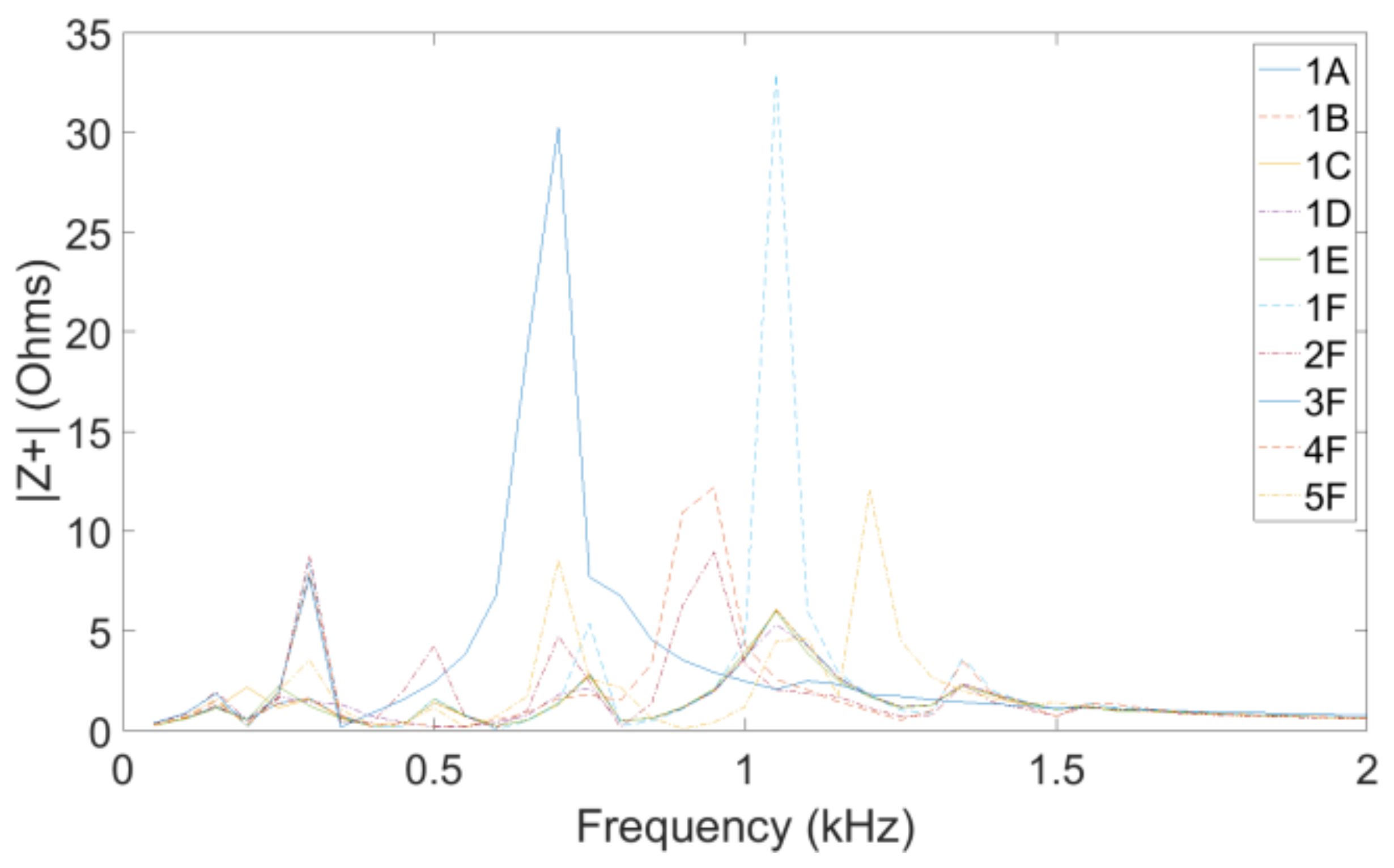
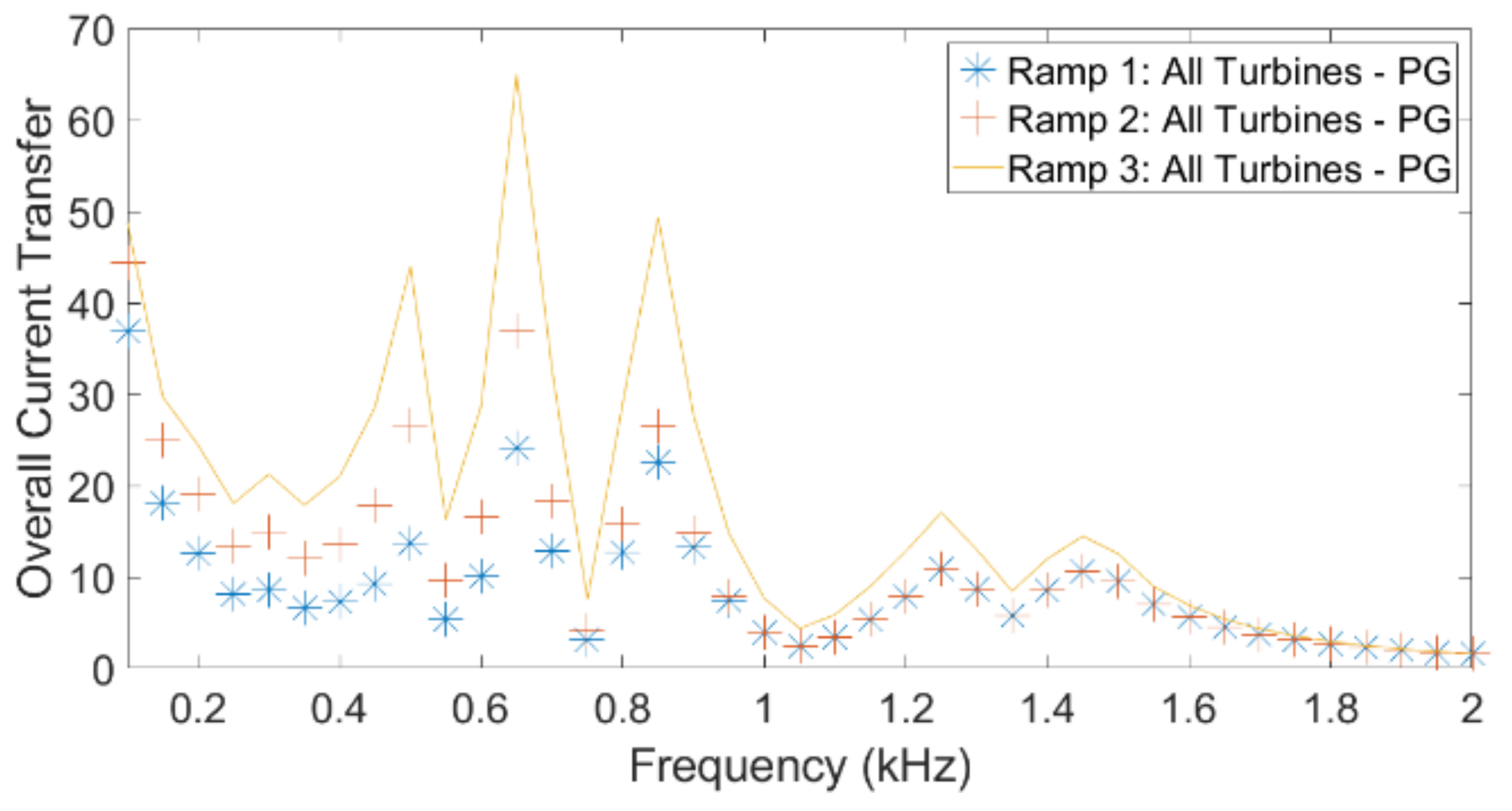
A general observation is that the difference due to the public grid impedance can vary a lot between neighbouring harmonics. This was also visible in, among others, Figure 23 and Figure 24. The difference in frequency values different operational states of the grid (i.e., for interharmonics) may be much bigger for interharmonics than for harmonics. Further studies are needed to verify this. In addition, small shifts in resonant frequency in the transmission grid, which could result in large changes in the public grid impedance at certain harmonics, could have a big impact on the transfers.

A general conclusion is that for studies about connecting WPPs into the power system, proper models and data should be used. The WT impedance and the public grid impedance have been shown to be important elements when modelling a WPP for harmonic or resonance studies, so more studies are needed on these topics.

4.3. General Findings and Recommendations

It is illustrated in this paper that the transfer function method is a useful tool for the study of harmonic propagation in and around WPPs. The use of the transfer function method makes it possible to study harmonic propagation and the risk of high distortion levels without detailed knowledge of the emission from individual turbines. The use of this method also allows an estimation of the relative influence of secondary emission, without detailed knowledge of primary emission. From the study of the two WPPs, it is concluded that secondary emission plays an important role and that it cannot be neglected. Because of this, it is difficult to interpret measurements of harmonic emission in WPPs; any measured emission will be a combination of primary and secondary emissions. Further work is needed towards the interpretation of measurements at locations where high levels of secondary emission are expected.

Calculation of transfer functions requires impedance data over the frequency range of interest. In this paper, the frequencies of interest were limited to the harmonic orders 2 to 40 (100 Hz to 2 kHz). The method can be applied to any frequency range, including interharmonics and supraharmonics.

Within the impedance data, distinction is needed between impedances of components within the collection grid, impedance data of the public grid and turbine impedance. Sufficient experience exists in studies in the harmonic frequency range to model the collection grid. For the public grid, the challenge is in the modelling the load impedance, especially its contribution to the damping at resonant frequencies. This challenge is not specific for wind power studies, but a general issue in harmonic propagation studies. The main modelling challenge is in finding a suitable impedance versus frequency for the turbines. Further research on this is needed, for example, to study the impact of the operational state of the turbine (the produced power) on the impedance. This further research should also include estimating to which extent a linear model (as has been used here) is appropriate for this. When performing harmonic studies during the design stage of a WPP, details of the turbines are not always available. This limits the accuracy of the WT impedance model. However, in the existing approach, the uncertainty in emission has a much bigger impact on the results than the uncertainty in the WT impedance.

Finally, for calculating the overall transfer functions, an aggregation model is needed. This is another subject where further work is needed, both for the transfer function approach and for existing methods.

5. Conclusions

The use of transfer functions allows harmonic propagation studies without knowledge of the emission from individual turbines or the background voltage distortion; transfer functions should find a broader application in both practical connection studies and research and education on harmonic propagation. The main challenge for future studies is in obtaining relevant models for the turbine impedance versus frequency. This is, however, less of an uncertainty for the results from a study than the uncertainty in turbine emission and background voltage distortion in the existing study methods.

References

1. Chen, Z.; Spooner, E. Grid power quality with variable speed wind turbines. IEEE Trans. Energy Convers. 2001, 16, 148–154. [Google Scholar] [CrossRef]
2. Papathanassiou, S.; Papadopoulos, M. Harmonic Analysis in a Power System with Wind Generation. IEEE Trans. Power Deliv. 2006, 21, 2006–2016. [Google Scholar] [CrossRef]
3. LaRose, C.; Gagnon, R.; Prud’Homme, P.; Fecteau, M.; Asmine, M. Type-III Wind Power Plant Harmonic Emissions: Field Measurements and Aggregation Guidelines for Adequate Representation of Harmonics. IEEE Trans. Sustain. Energy 2013, 4, 797–804. [Google Scholar] [CrossRef]
4. Tentzerakis, S.T.; Papathanassiou, S.A. An Investigation of the Harmonic Emissions of Wind Turbines. IEEE Trans. Energy Convers. 2007, 22, 150–158. [Google Scholar] [CrossRef]
5. Thiringer, T. Power quality measurements performed on a low-voltage grid equipped with two wind turbines. IEEE Trans. Energy Convers. 1996, 11, 601–606. [Google Scholar] [CrossRef]
6. Mohod, S.W.; Aware, M.V. A STATCOM-control scheme for grid connected wind energy system for power quality improvement. IEEE Syst. J. 2010, 4, 346–352. [Google Scholar] [CrossRef]
7. Melicio, R.; Mendes, V.; Catalão, J. Comparative study of power converter topologies and control strategies for the harmonic performance of variable-speed wind turbine generator systems. Energy 2011, 36, 520–529. [Google Scholar] [CrossRef]
8. Hasan, K.N.B.M.; Rauma, K.; Luna, A.; Candela, J.I.; Rodriguez, P.; García, J.I.C. Harmonic Compensation Analysis in Offshore Wind Power Plants Using Hybrid Filters. IEEE Trans. Ind. Appl. 2013, 50, 2050–2060. [Google Scholar] [CrossRef]
9. Chen, Z. Compensation Schemes for a SCR Converter in Variable Speed Wind Power Systems. IEEE Trans. Power Deliv. 2004, 19, 813–821. [Google Scholar] [CrossRef]
10. Gaillard, A.; Poure, P.; Saadate, S.; Machmoum, M. Variable speed DFIG wind energy system for power generation and harmonic current mitigation. Renew. Energy 2009, 34, 1545–1553. [Google Scholar] [CrossRef]
11. Teodorescu, R.; Liserre, M.; Rodriguez, P. Grid Converters for Photovoltaic and Wind Power Systems; John Wiley & Sons: Hoboken, NJ, USA, 2011; Volume 29. [Google Scholar]
12. Li, J.; Bhattacharya, S.; Huang, A.Q. A New Nine-Level Active NPC (ANPC) Converter for Grid Connection of Large Wind Turbines for Distributed Generation. IEEE Trans. Power Electron. 2011, 26, 961–972. [Google Scholar] [CrossRef]
13. IEEE. IEEE 519-2014, IEEE Recommended Practice and Requirements for Harmonic Control in Electric Power Systems; IEEE: Piscataway, NJ, USA, 2014. [Google Scholar]
14. IEC. IEC 61000-3-6: 2008, Electromagnetic Compatibility (EMC)-Part 3-6: Limits—Assessment of Emission Limits for the Connection of Distorting Installations to MV, HV and EHV Power Systems; IEC: London, UK, 2008. [Google Scholar]
15. IEC. IEC 61400-21-3: 2019, Wind Energy Generation Systems-Part 21-3: Measurement and Assessment of Electrical Characteristics—Wind Turbine Harmonic Model and Its Application; IEC: London, UK, 2019. [Google Scholar]
16. Andresen, B.; Christensen, L.; Srypalle, I.; Kocewiak, L.H.; Santjer, F. Overview, status and outline of the new standard series—IEC 61400-21. In Proceedings of the 14th Int Workshop on Large-Scale Integration of Wind Power into the Power System as well as on Transmission Networks for Offshore Wind Power Plants, Brussels, Belgium, 20–22 October 2015. [Google Scholar]
17. Meyer, J.; Bollen, M.; Amaris, H.; Blanco, A.M.; Gil de Castro, A.; Desmet, J.; Klatt, M.; Kocewiak, L.; Ronnberg, S.; Yang, K. Future work on harmonics-some expert opinions Part II—Supraharmonics, standards and measurements. In Proceedings of the 2014 16th International Conference on Harmonics and Quality of Power (ICHQP), Bucharest, Romania, 25–28 May 2014; IEEE: Piscataway, NJ, USA, 2014; pp. 909–913. [Google Scholar]
18. Badrzadeh, B.; Gupta, M.; Singh, N.; Petersson, A.; Max, L.; Høgdahl, M. Power system harmonic analysis in wind power plants—Part I: Study methodology and techniques. In Proceedings of the 2012 IEEE Industry Applications Society Annual Meeting, Las Vegas, NV, USA, 7–11 October 2012; IEEE: Piscataway, NJ, USA, 2012; pp. 1–11. [Google Scholar]
19. Shafiu, A.; Hernandez, A.; Schettler, F.; Finn, J.; Jørgensen, E. Harmonic studies for offshore windfarms. In Proceedings of the 9th IET International Conference on AC and DC Power Transmission (ACDC 2010), London, UK, 19–21 October 2010; Institution of Engineering and Technology: London, UK, 2010. [Google Scholar]
20. Koo, K.L. Harmonic assessments for filter design specifications at U.K. National Grid electricity transmission system for large wind farms. In Proceedings of the 45th International Universities Power Engineering Conference (UPEC), Cardiff, UK, 31 August–3 September 2010. [Google Scholar]
21. Vazquez, R.; Muñoz, M.; Alonso, M.; Amaris, H.; Alvarez, C. Background harmonic distortion measurement at power networks with wind farms. Renew. Energy Power Qual. J. 2016, 873–878. [Google Scholar] [CrossRef]
22. Bradt, M.; Badrzadeh, B.; Camm, E.; Mueller, D.; Schoene, J.; Siebert, T.; Smith, T.; Starke, M.; Walling, R. Harmonics and resonance issues in wind power plants. In Proceedings of the IEEE PES Transmission and Distribution Conference and Exposition (T&D 2012), Orlando, FL, USA, 7–10 May 2012. [Google Scholar]
23. Chen, Y.; Bollen, M.; Martins, M. Application of transfer function based harmonic study method to an offshore wind farm. In Proceedings of the 11th International Workshop on Large-Scale Integration of Wind Power into the Power System as Well as on Transmission Networks for Offshore Wind Power Plants, Lisbon, Portugal, 13–15 November 2012. [Google Scholar]
24. Ravindran, V.; Nakhodchi, N.; Ronnberg, S.; Bollen, M.H.J. Assessing Time-Varying Harmonic Interactions in a Wind Park. IEEE Access 2021, 9, 68151–68160. [Google Scholar] [CrossRef]
25. Schwanz, D.; Bollen, M. Harmonic limits in connection agreement for wind power plants. In Advances in Renewable Energies and Power Quality; Pérez-Donsión, M., Vitale, G., Eds.; Cambridge Scholars Publishing: Newcastle upon Tyne, UK, 2020. [Google Scholar]
26. Sainz, L.; Mesas, J.J.; Teodorescu, R.; Rodriguez, P. Deterministic and Stochastic Study of Wind Farm Harmonic Currents. IEEE Trans. Energy Convers. 2010, 25, 1071–1080. [Google Scholar] [CrossRef] [Green Version]
27. Rönnberg, S.; Larsson, A.; Bollen, M.; Schanen, J.L. A simple model for interaction between equipment at a frequency of some tens of kHz. In Proceedings of the International Conference Electricity Distribution (CIRED), Frankfurt, Germany, 6–9 June 2011. [Google Scholar]
28. Yang, K. Wind-Turbine Harmonic Emissions and Propagation through a Wind Farm. Ph.D. Thesis, Department of Engineering, Sciences and Mathematics, Luleå University of Technology, Skellefteå, Sweden, 2012. [Google Scholar]
29. Bollen, M.H.J.; Rönnberg, S.K. Primary and secondary harmonics emission; harmonic interaction—A set of definitions. In Proceedings of the 17th International Conference on Harmonics and Quality of Power (ICHQP), Belo Horizonte, Brazil, 16–19 October 2016; pp. 703–708. [Google Scholar]
30. Zavoda, F.; (Convenor). CIGRE C4.24, Power quality and EMC issues with future electricity networks. In CIGRE Technical Brochure; CIGRE: Paris, France, 2018; p. 719. [Google Scholar]
31. Yang, K. On Harmonic Emission, Propagation and Aggregation in Wind Power Plants. Ph.D. Thesis, Department of Engineering, Sciences and Mathematics, Luleå University of Technology, Skellefteå, Sweden, 2015. [Google Scholar]
32. Yang, K.; Bollen, M.H.; Amaris, H.; Alvarez, C. Decompositions of harmonic propagation in wind power plant. Electr. Power Syst. Res. 2016, 141, 84–90. [Google Scholar] [CrossRef]
33. Schwanz, D.; Bollen, M.; Larsson, A. Some methods for harmonic emission determination in wind power plants. In Proceedings of the 2018 18th International Conference on Harmonics and Quality of Power (ICHQP), Ljubljana, Slovenia, 13–16 May 2018; Institute of Electrical and Electronics Engineers (IEEE): Piscataway, NJ, USA, 2018; pp. 1–6. [Google Scholar]
34. Ebrahimzadeh, E.; Blaabjerg, F.; Wang, X.; Bak, C.L. Harmonic Stability and Resonance Analysis in Large PMSG-Based Wind Power Plants. IEEE Trans. Sustain. Energy 2017, 9, 12–23. [Google Scholar] [CrossRef]
35. Do, V.Q.; Gavrilovic, M.M. A Synthesis Method for One-Port and Multi-Port Equivalent Networks for Analysis of Power System Transients. IEEE Trans. Power Deliv. 1986, 1, 103–113. [Google Scholar] [CrossRef]
36. Mollerstedt, E.; Bernhardsson, B. A harmonic transfer function model for a diode converter train. In Proceedings of the 2000 IEEE Power Engineering Society Winter Meeting. Conference Proceedings (Cat. No.00CH37077), Singapore, 23–27 January 2000; Institute of Electrical and Electronics Engineers (IEEE): Piscataway, NJ, USA, 2002; Volume 2, pp. 957–962. [Google Scholar]
37. Vanassche, P.; Gielen, G.; Sansen, W. Symbolic modeling of periodically time-varying systems using harmonic transfer matrices. IEEE Trans. Comput. Des. Integr. Circuits Syst. 2002, 21, 1011–1024. [Google Scholar] [CrossRef]
38. Bakhshizadeh, M.K.; Blaabjerg, F.; Hjerrild, J.; Wang, X.; Kocewiak, L.; Bak, C.L. A Numerical Matrix-Based Method for Stability and Power Quality Studies Based on Harmonic Transfer Functions. IEEE J. Emerg. Sel. Top. Power Electron. 2017, 5, 1542–1552. [Google Scholar] [CrossRef]
39. Yang, Y.; Bollen, M.; Yao, L. Theoretical emission study of wind park grids: Emission propagation between wind park and grid. In Proceedings of the 11th International Conference on Electric Power Quality and Utilization, Lisbon, Portugal, 17–19 October 2011. [Google Scholar]
40. Yang, K.; Bollen, M.H.J.; Larsson, E.O.A. Aggregation and Amplification of Wind-Turbine Harmonic Emission in a Wind Park. IEEE Trans. Power Deliv. 2015, 30, 791–799. [Google Scholar] [CrossRef]
41. Shi, J.; Chen, W.; Pei, X.; Wei, Z.; Sun, X. Analysis for action degree and influence factors of harmonic interaction in multi-wind farms. J. Renew. Sustain. Energy 2021, 13, 045301. [Google Scholar] [CrossRef]
42. Guest, E.; Jensen, K.H.; Rasmussen, T.W. Probabilistic harmonic modeling of wind power plants. In Proceedings of the 16th International Workshop on Large-Scale Integration of Wind Power into Power Systems as well as on Transmission Networks for Offshore Wind Power Plants, Energynautics, Berlin, Germany, 25–27 October 2017. [Google Scholar]
43. Andres de Jesus Arguello, G. Resonance Assessment in Power Systems with DFIG-Based Wind Parks. Ph.D. Dissertation, School of Electrical and Computer Engineering of the State University of Campinas, Campinas, Brazil, 2019. [Google Scholar]
44. Shi, J.; Chen, W.; Pei, X.; Zheng, G.; Wang, K. Research on Harmonic Resonance Mechanism and Characteristics for Power System with High Proportion of Renewable Energy. In International Conference on Communication, Computing and Electronics Systems; Springer Science and Business Media LLC: Berlin/Heidelberg, Germany, 2021; pp. 301–313. [Google Scholar]
45. King, R.; Ekanayake, J.B. Harmonic modelling of offshore wind farms. In Proceedings of the IEEE Power and Energy Society General Meeting, Minneapolis, MN, USA, 25–29 July 2010. [Google Scholar] [CrossRef]
46. Dugan, R.; McGranaghan, M.; Santoso, S.; Beaty, H. Electrical Power Systems Quality, 2nd ed.; McGraw-Hill: New York, NY, USA, 2002; pp. 225–294. [Google Scholar]
47. Madrigal, M.; Acha, E. Modelling of custom power equipment using harmonic domain techniques. In Proceedings of the Ninth International Conference on Harmonics and Quality of Power. Proceedings (Cat. No.00EX441), Orlando, FL, USA, 1–4 October 2000; Institute of Electrical and Electronics Engineers (IEEE): Piscataway, NJ, USA, 2002; pp. 264–269. [Google Scholar]
48. Sainz, L.; Monjo, L.; Pedra, J.; Cheah-Mane, M.; Liang, J.; Gomis-Bellmunt, O. Effect of wind turbine converter control on wind power plant harmonic response and resonances. IET Electr. Power Appl. 2017, 11, 157–168. [Google Scholar] [CrossRef]
49. Yang, K.; Bollen, M.; Wahlberg, M. Comparison of harmonic emissions at two nodes in a windpark. In Proceedings of the 2012 IEEE 15th International Conference on Harmonics and Quality of Power, Hong Kong, China, 17–20 June 2012; IEEE: Piscataway, NJ, USA, 2012; pp. 313–319. [Google Scholar]
Figure 1. WPP as a multi-port network; each transfer function considers the transfer from one port to another, with a given termination of the other ports.
Energies 14 05798 g001
Figure 2. Wind turbine impedance as a function of frequency, as used in this paper.
Energies 14 05798 g002
Figure 3. Overall transfer admittance (A/V) from turbine to public grid: 5-turbine plant.
Energies 14 05798 g003
Figure 4. Overall transfer admittance (A/V) from turbine to public grid: 42-turbine plant.
Energies 14 05798 g004
Figure 5. Overall transfer admittance (A/V) between turbines: 5-turbine plant.
Energies 14 05798 g005
Figure 6. Overall transfer admittance (A/V) between turbines: 42-turbine plant.
Energies 14 05798 g006
Figure 7. Overall current transfer between turbines: 5-turbine plant.
Energies 14 05798 g007
Figure 8. Overall current transfer between turbines: 42-turbine plant.
Energies 14 05798 g008
Figure 9. Transfer admittance (A/V) from public grid to turbines: 5-turbine wind power plant.
Energies 14 05798 g009
Figure 10. Transfer admittance (A/V) from public grid to turbines: 42-turbine wind power plant.
Energies 14 05798 g010
Figure 11. Impact of aggregation exponent on overall current transfer from turbines to public grid: 42-turbine wind power plant.
Energies 14 05798 g011
Figure 12. Impact of aggregation exponent on overall transfer admittance from turbines to public grid: 42-turbine wind power plant.
Energies 14 05798 g012
Figure 13. Impact of WT impedance on overall transfer admittance from all turbines to one turbine: 5-turbine wind power plant.
Energies 14 05798 g013
Figure 14. Impact of WT impedance on overall transfer admittance from all turbines to one turbine: 42-turbine wind power plant.
Energies 14 05798 g014
Figure 15. Impact of wind-turbine impedance on overall transfer admittance (A/V) from turbine to public grid: 5-turbine wind power plant.
Energies 14 05798 g015
Figure 16. Impact of wind turbine impedance on overall transfer admittance (A/V) from turbine to public grid: 42-turbine wind power plant.
Energies 14 05798 g016
Figure 17. Difference (%) due to WT impedance: transfer admittance (A/V) from all turbines to one turbine (T1) in 5- and 42-turbine cases.
Energies 14 05798 g017
Figure 18. Difference (%) due to WT impedance: transfer admittance (A/V) from all turbines to the public grid in 5- and 42-turbine cases.
Energies 14 05798 g018
Figure 19. Impact of public grid impedance on overall transfer admittance (A/V) from turbine to turbine: 5-turbine wind power plant.
Energies 14 05798 g019
Figure 20. Impact of public grid impedance on overall transfer admittance (A/V) from turbine to turbine: 42-turbine wind power plant.
Energies 14 05798 g020
Figure 21. Impact of public grid impedance on overall transfer admittance (A/V) from turbine to public grid: 5-turbine wind power plant.
Energies 14 05798 g021
Figure 22. Impact of public grid impedance on overall transfer admittance (A/V) from turbine to public grid: 42-turbine wind power plant.
Energies 14 05798 g022
Figure 23. Difference (%) due to public grid impedance: transfer admittance (A/V) from all turbines to one turbine (T1) in 5- and 42-turbine cases.
Energies 14 05798 g023
Figure 24. Difference (%) due to public grid impedance: overall transfer admittance (A/V) from all turbines to public grid in 5- and 42-turbine cases.
Energies 14 05798 g024