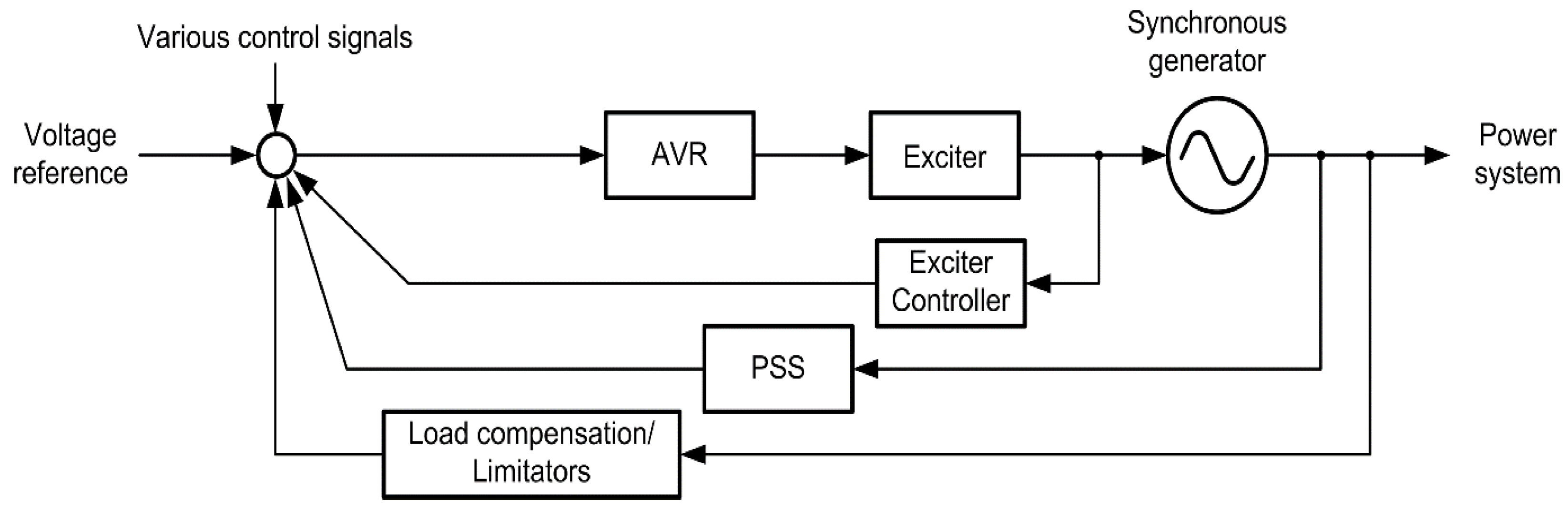
Figure 1.
Synchronous generator excitation system.
Figure 1.
Synchronous generator excitation system.
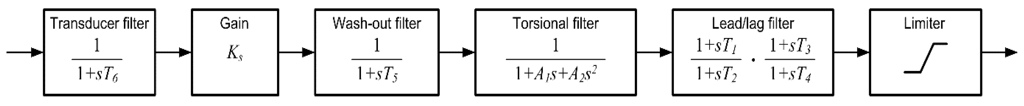
Figure 2.
Type PSS1A single-input power system stabilizer. Reproduced from [
39], Copyright 2016 IEEE.
Figure 2.
Type PSS1A single-input power system stabilizer. Reproduced from [
39], Copyright 2016 IEEE.
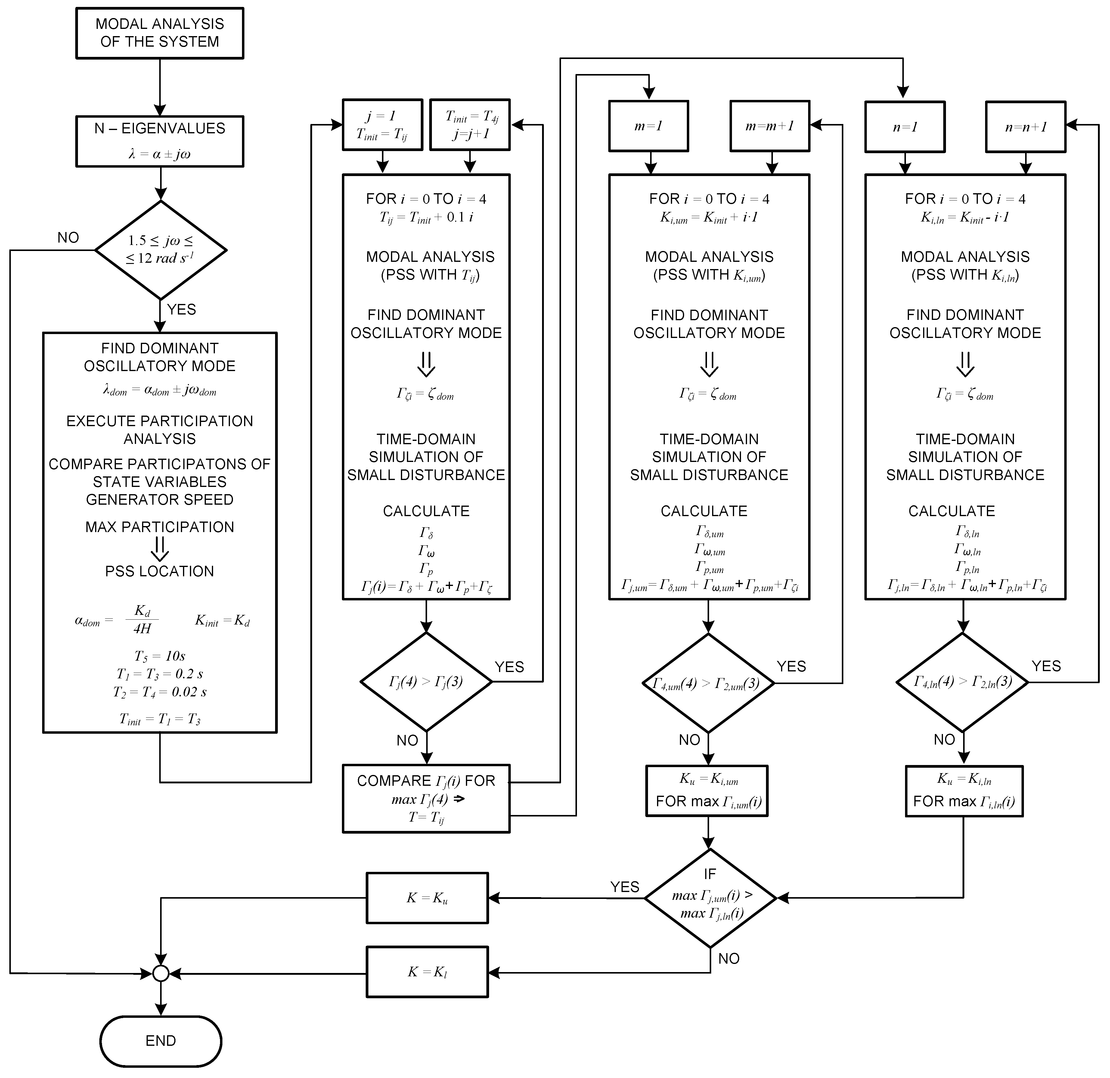
Figure 3.
PSS tuning algorithm.
Figure 3.
PSS tuning algorithm.
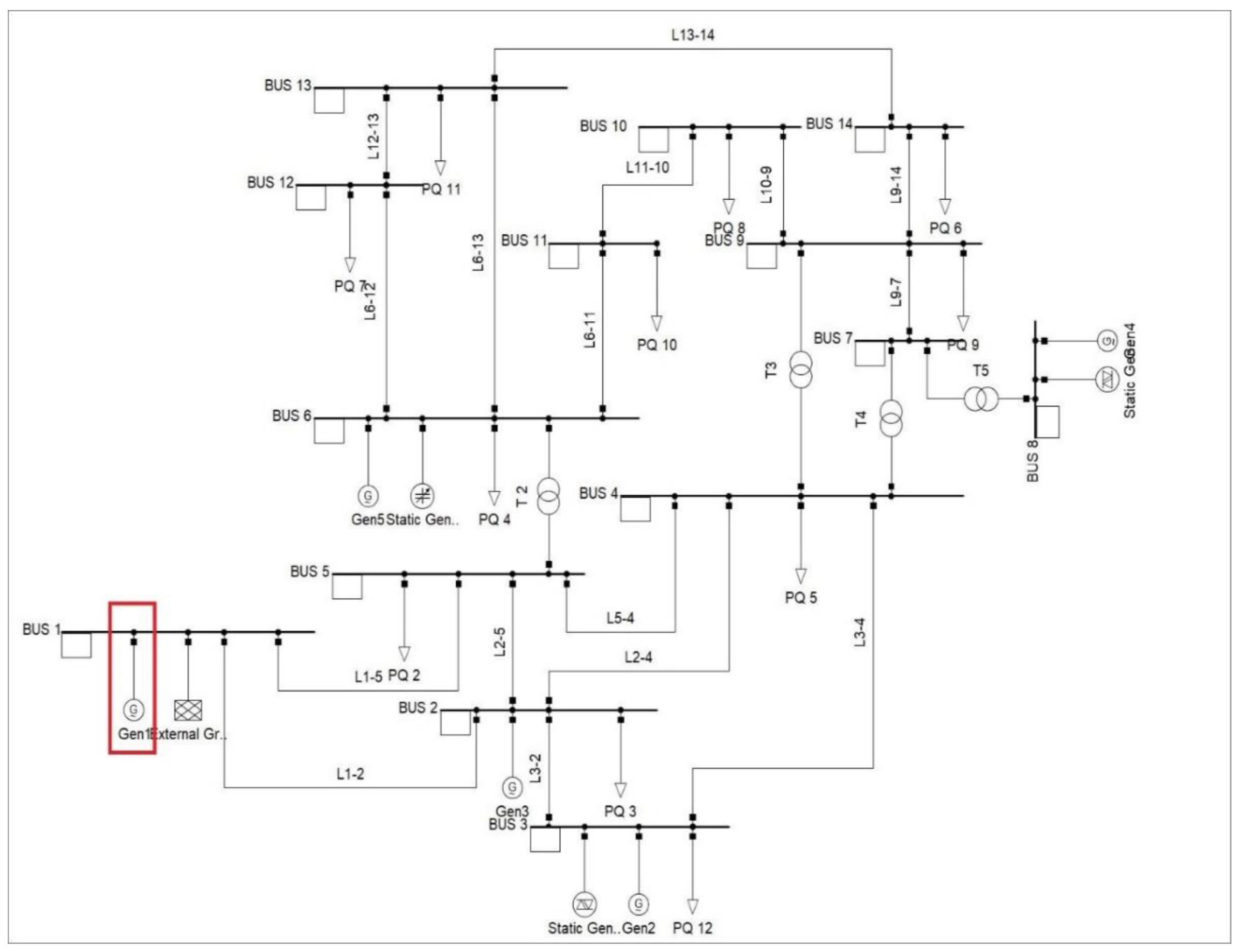
Figure 4.
IEEE 14 bus system model in DIgSILENT PowerFactory simulation interface.
Figure 4.
IEEE 14 bus system model in DIgSILENT PowerFactory simulation interface.
Figure 5.
Root locus diagram of the analyzed system without the PSS implementation.
Figure 5.
Root locus diagram of the analyzed system without the PSS implementation.
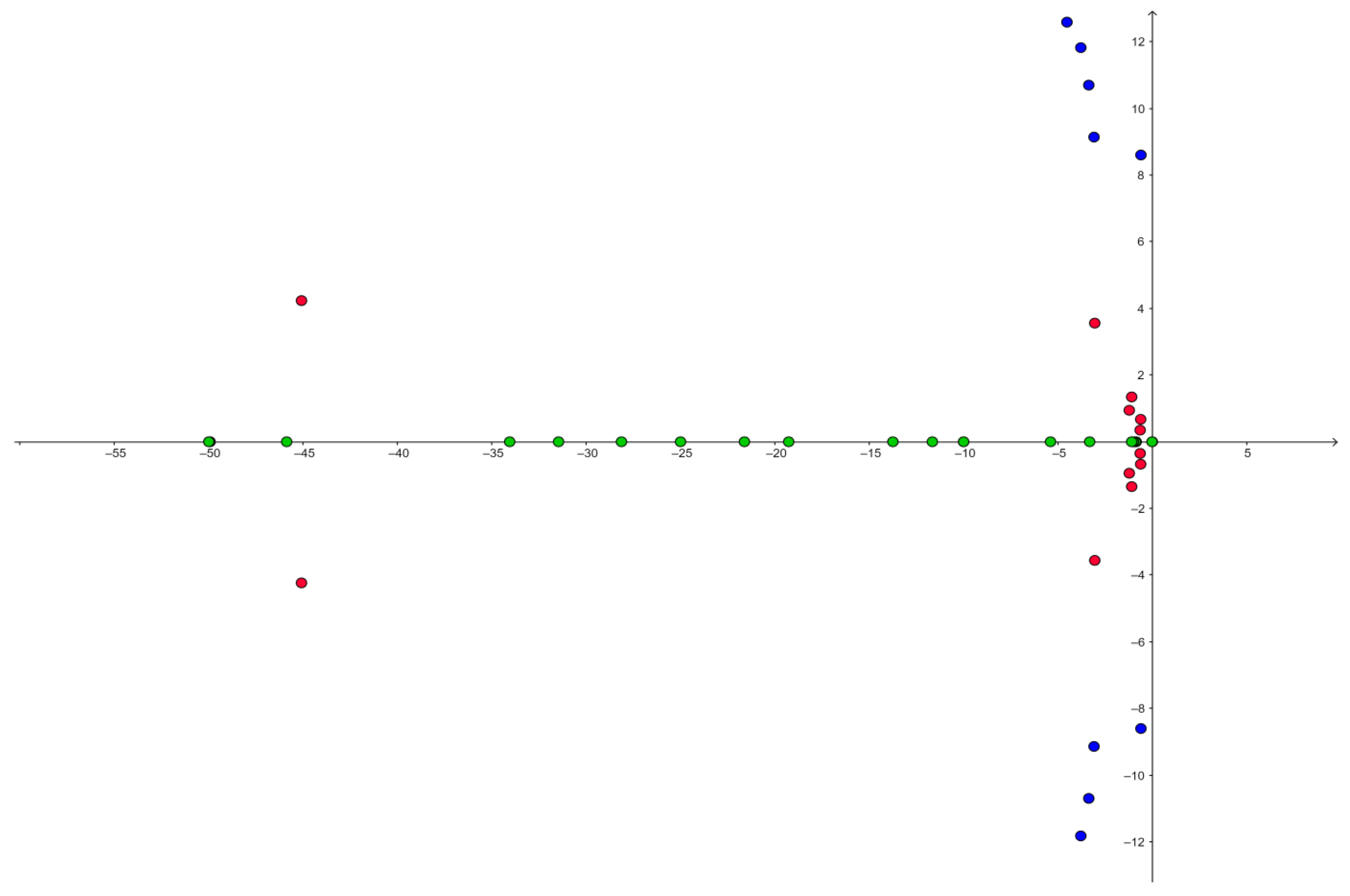
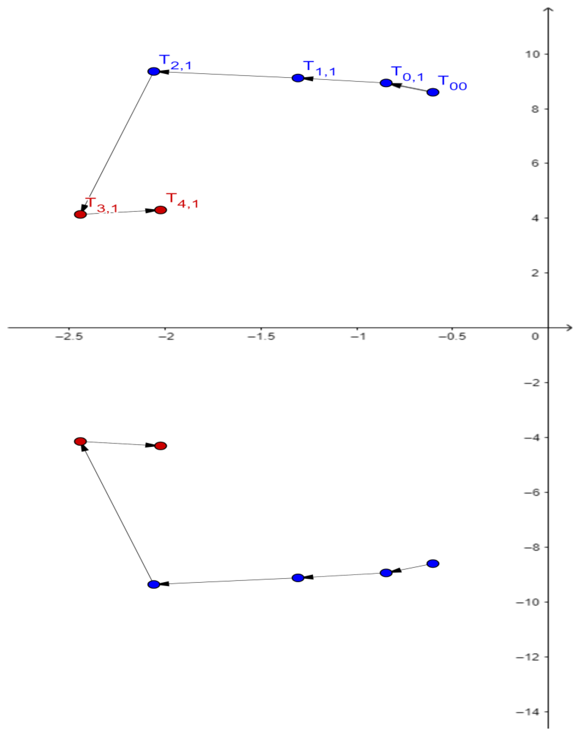
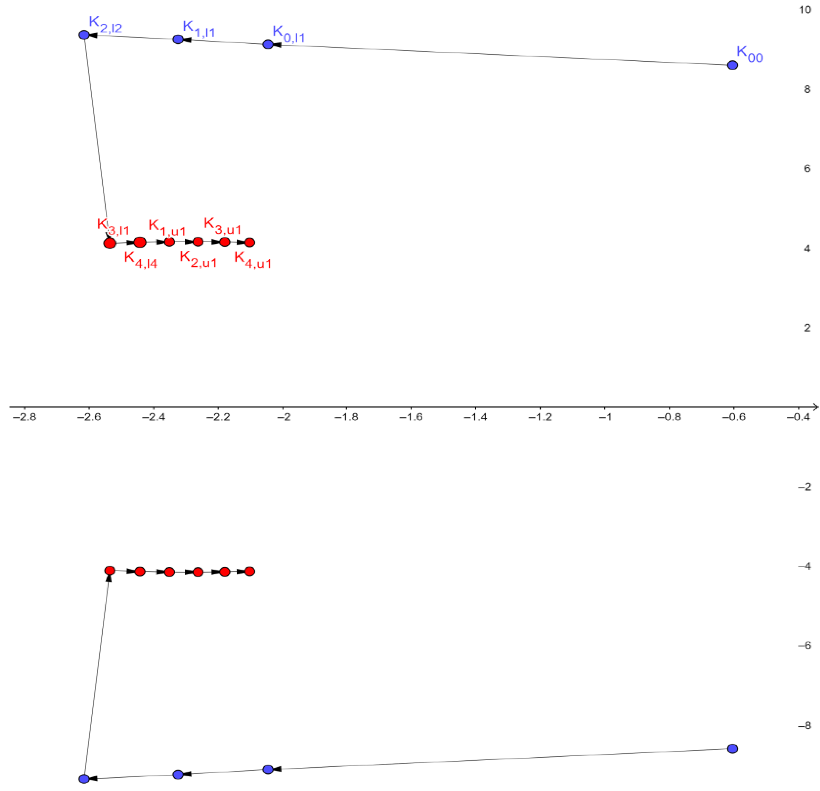
Figure 6.
Dominant oscillatory pole movement in the S-plane after the PSS implementation with K = 10 and the increasing time constants from T = 0.2 s to T = 0.6 s.
Figure 6.
Dominant oscillatory pole movement in the S-plane after the PSS implementation with K = 10 and the increasing time constants from T = 0.2 s to T = 0.6 s.
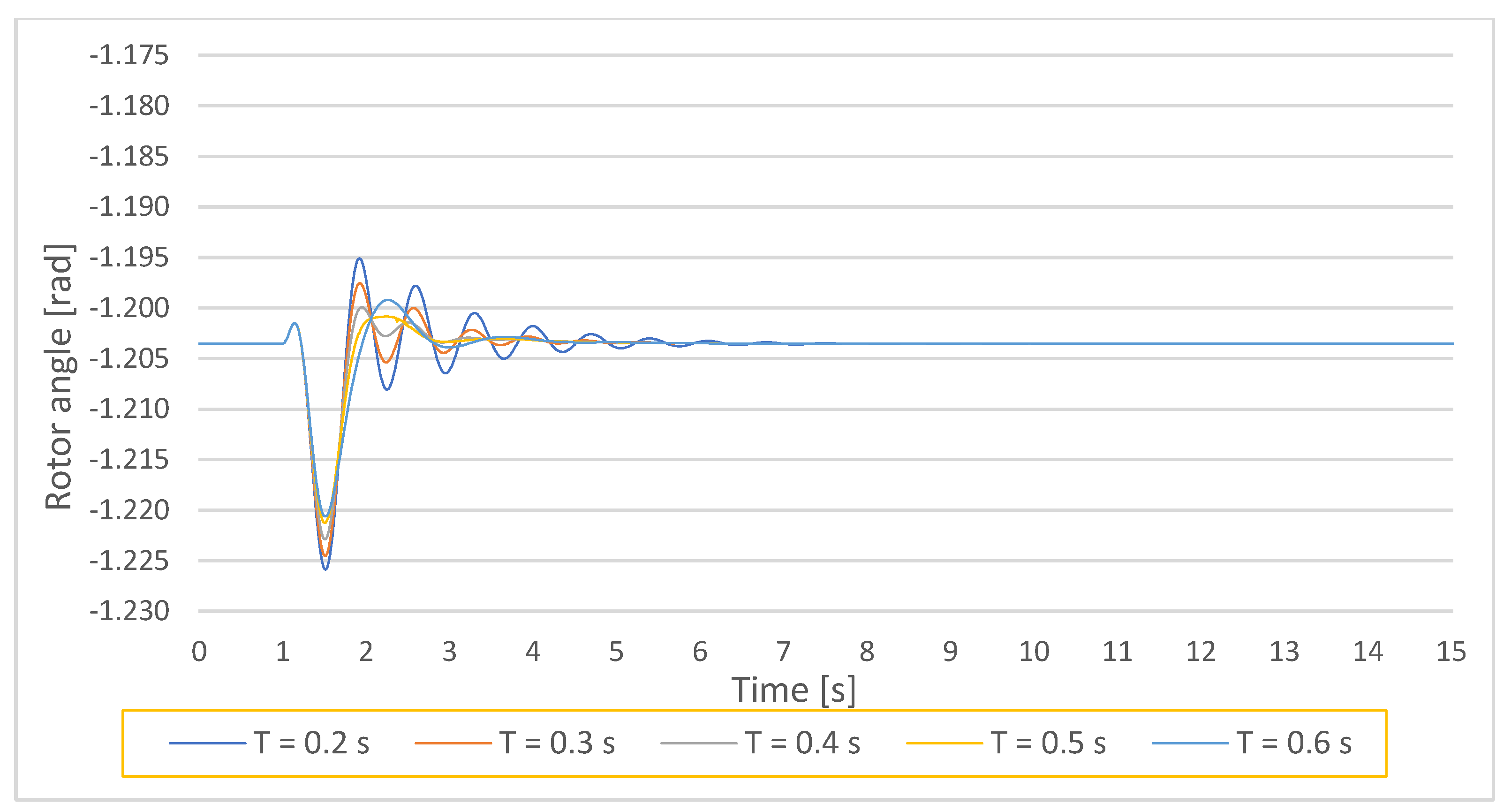
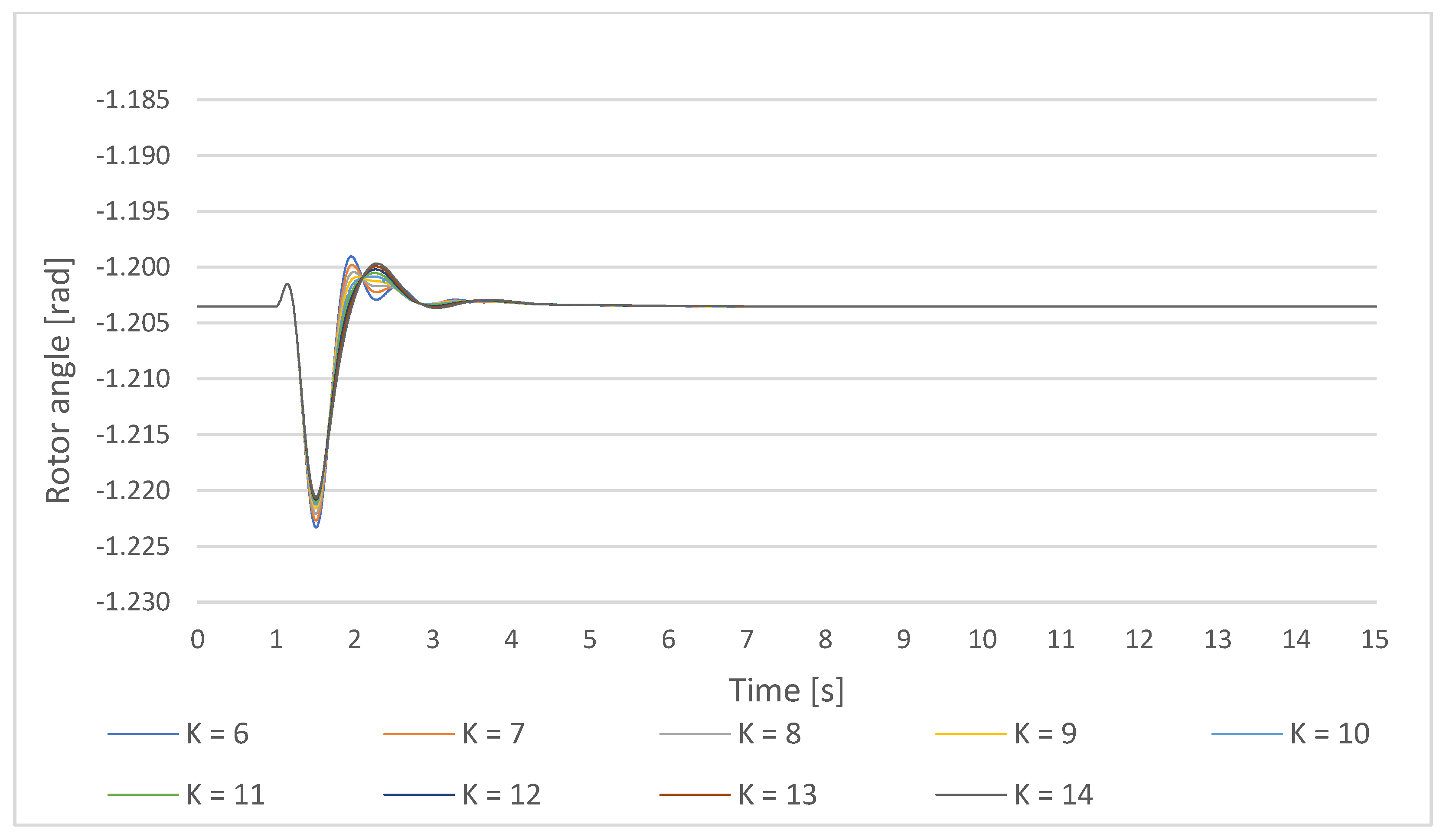
Figure 7.
Gen1 rotor angle response on a small disturbance with PSS parameters K = 10, and T = Ti,1 = 0.2–0.6 s.
Figure 7.
Gen1 rotor angle response on a small disturbance with PSS parameters K = 10, and T = Ti,1 = 0.2–0.6 s.
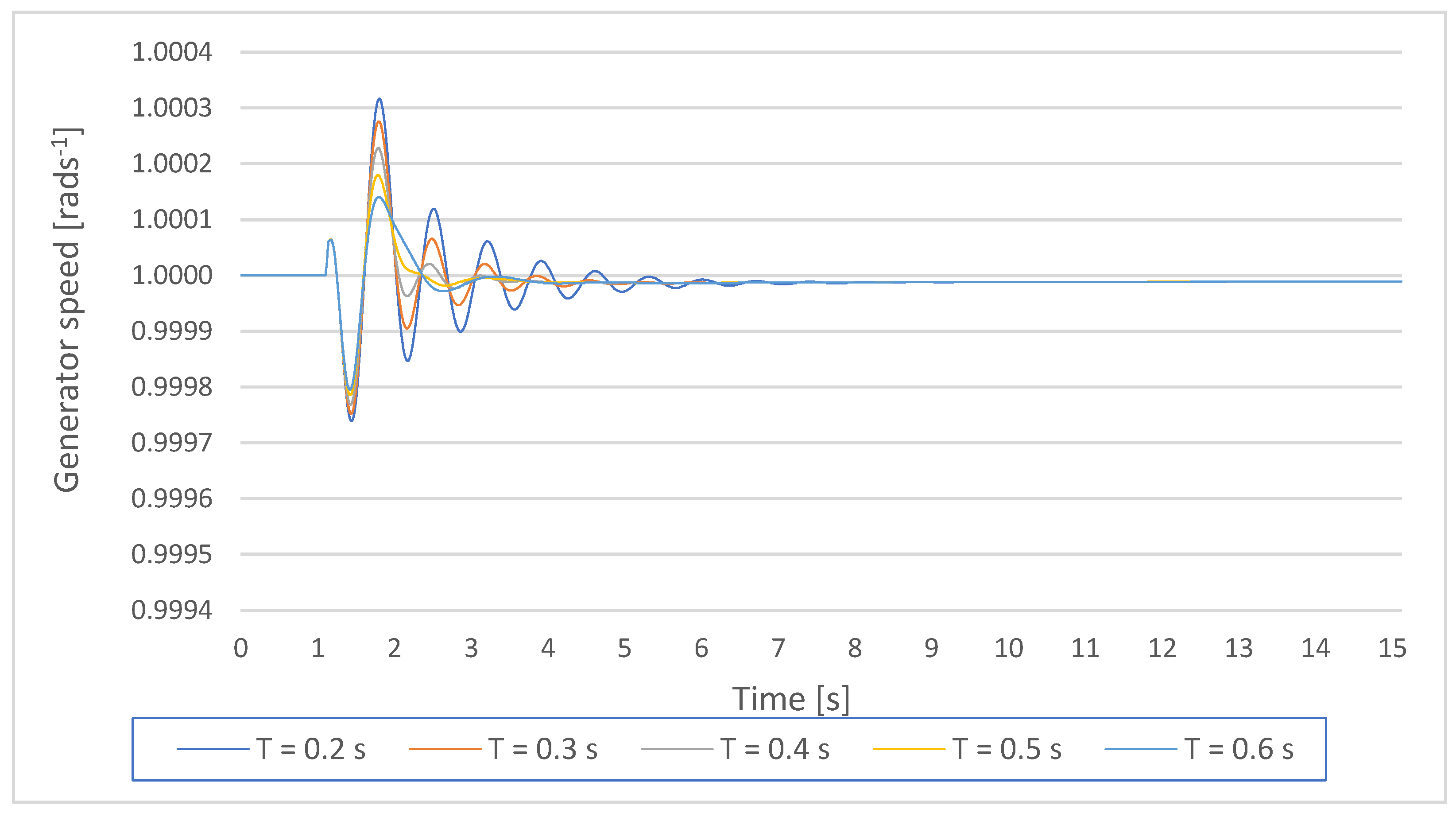
Figure 8.
Gen1 speed response on a small disturbance with PSS parameters K = 10, and T = Ti,1 = 0.2–0.6 s.
Figure 8.
Gen1 speed response on a small disturbance with PSS parameters K = 10, and T = Ti,1 = 0.2–0.6 s.
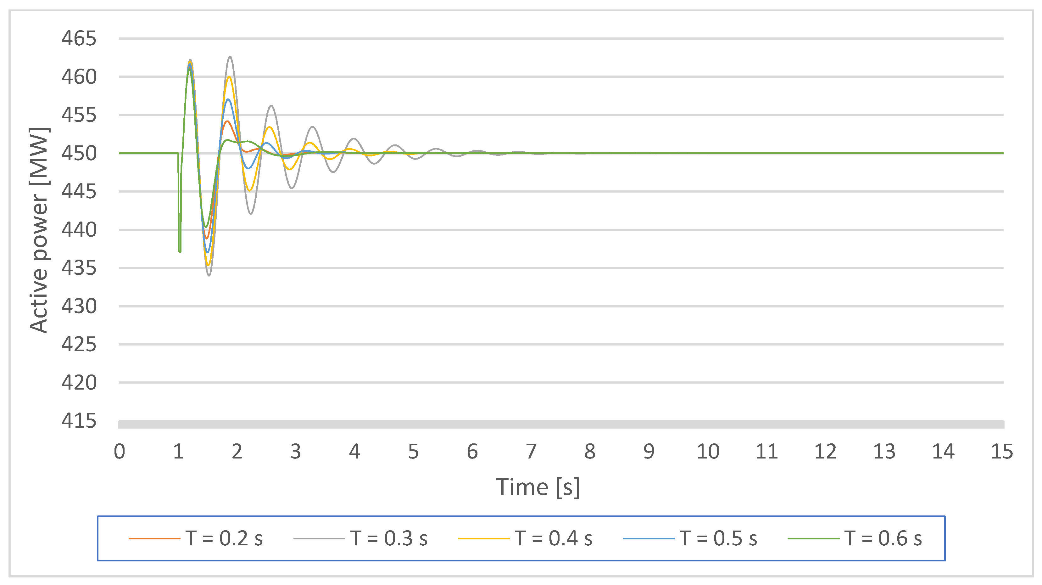
Figure 9.
Gen1 active power response on a small disturbance with PSS parameters K = 10, and T = Ti,1 = 0.2–0.6 s.
Figure 9.
Gen1 active power response on a small disturbance with PSS parameters K = 10, and T = Ti,1 = 0.2–0.6 s.
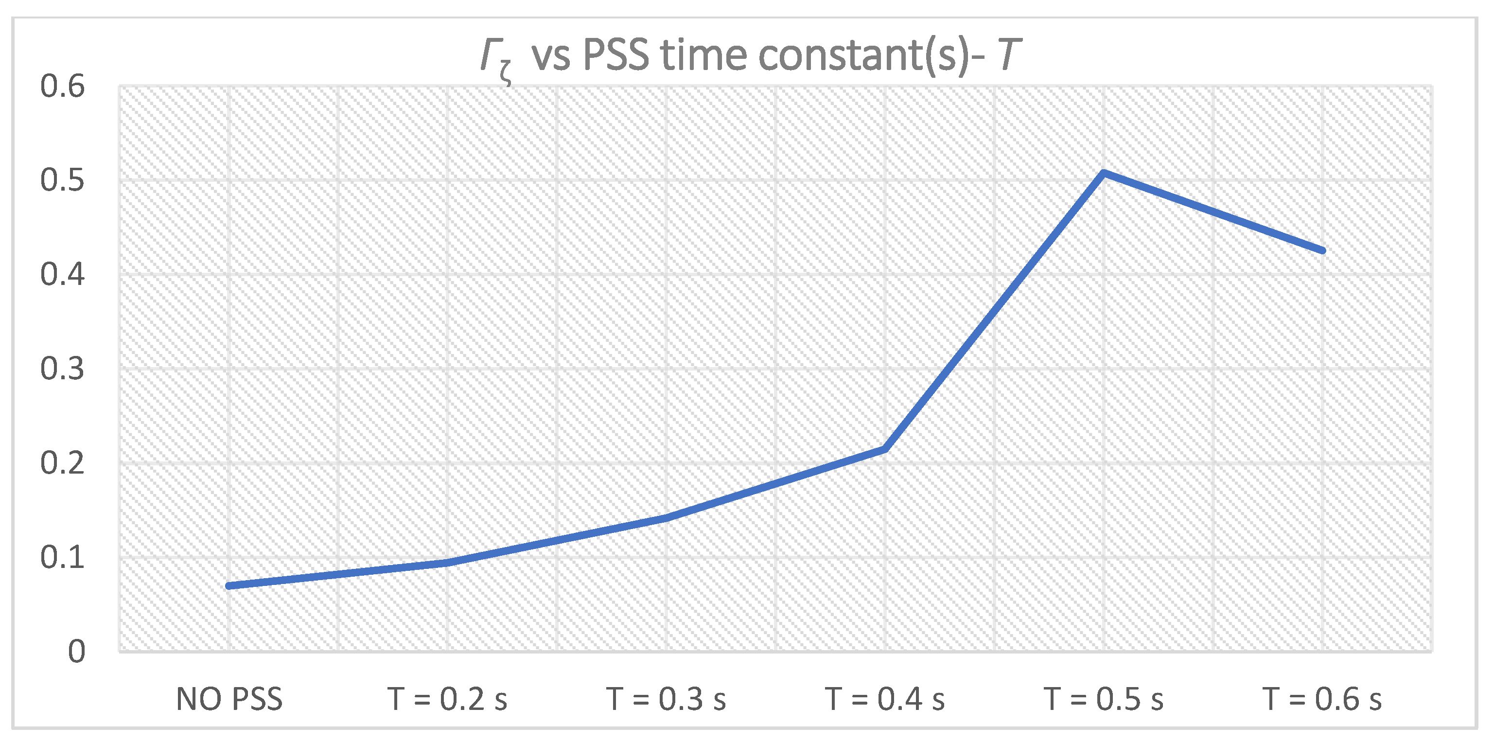
Figure 10.
Γζi for PSS parameters K = 10, T = Ti,1 = 0.2–0.6 s.
Figure 10.
Γζi for PSS parameters K = 10, T = Ti,1 = 0.2–0.6 s.
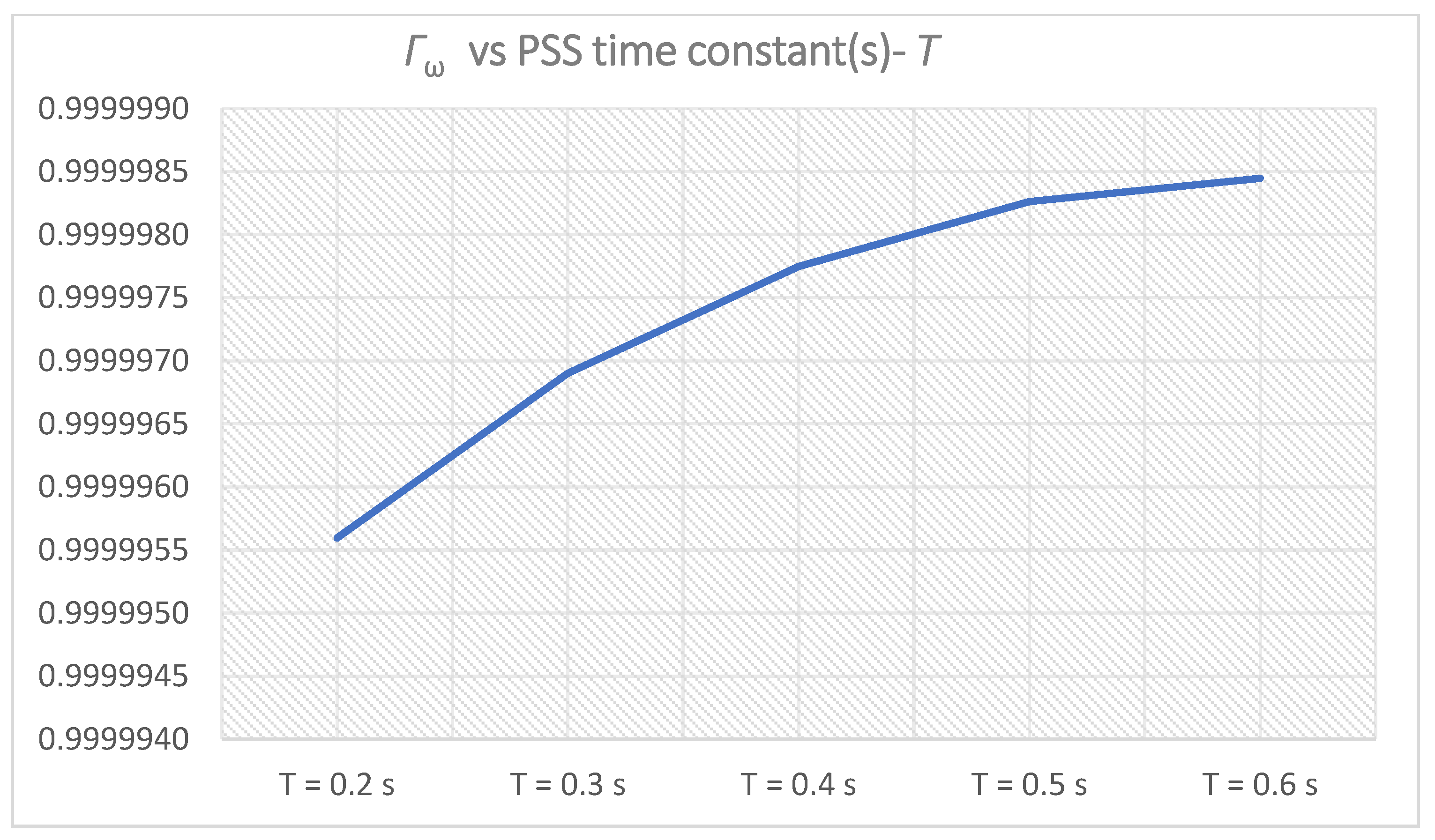
Figure 11.
Γωi for PSS parameters K = 10, T = Ti,1 = 0.2–0.6 s.
Figure 11.
Γωi for PSS parameters K = 10, T = Ti,1 = 0.2–0.6 s.
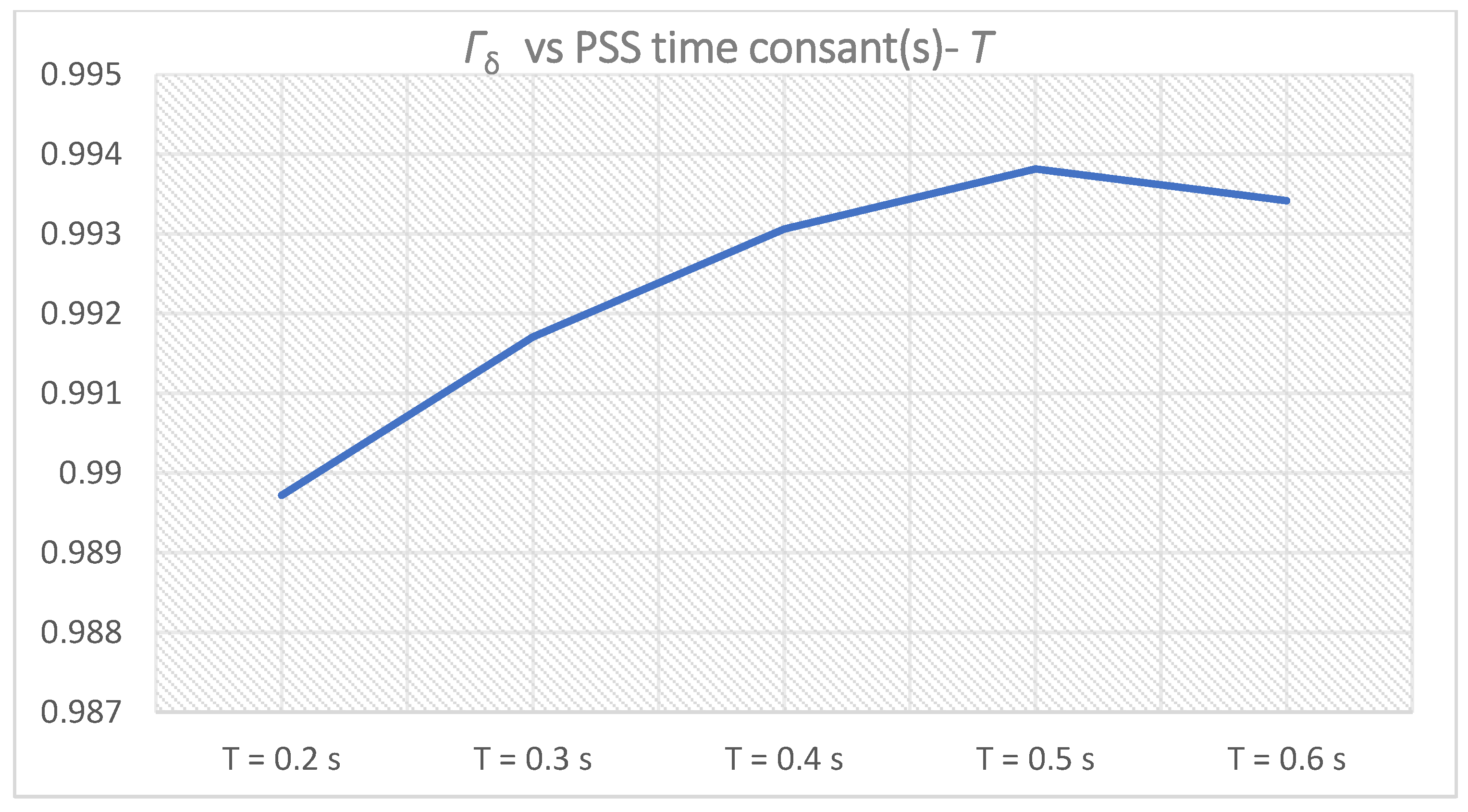
Figure 12.
Γδi for PSS parameters K = 10, T = Ti,1 = 0.2–0.6 s.
Figure 12.
Γδi for PSS parameters K = 10, T = Ti,1 = 0.2–0.6 s.
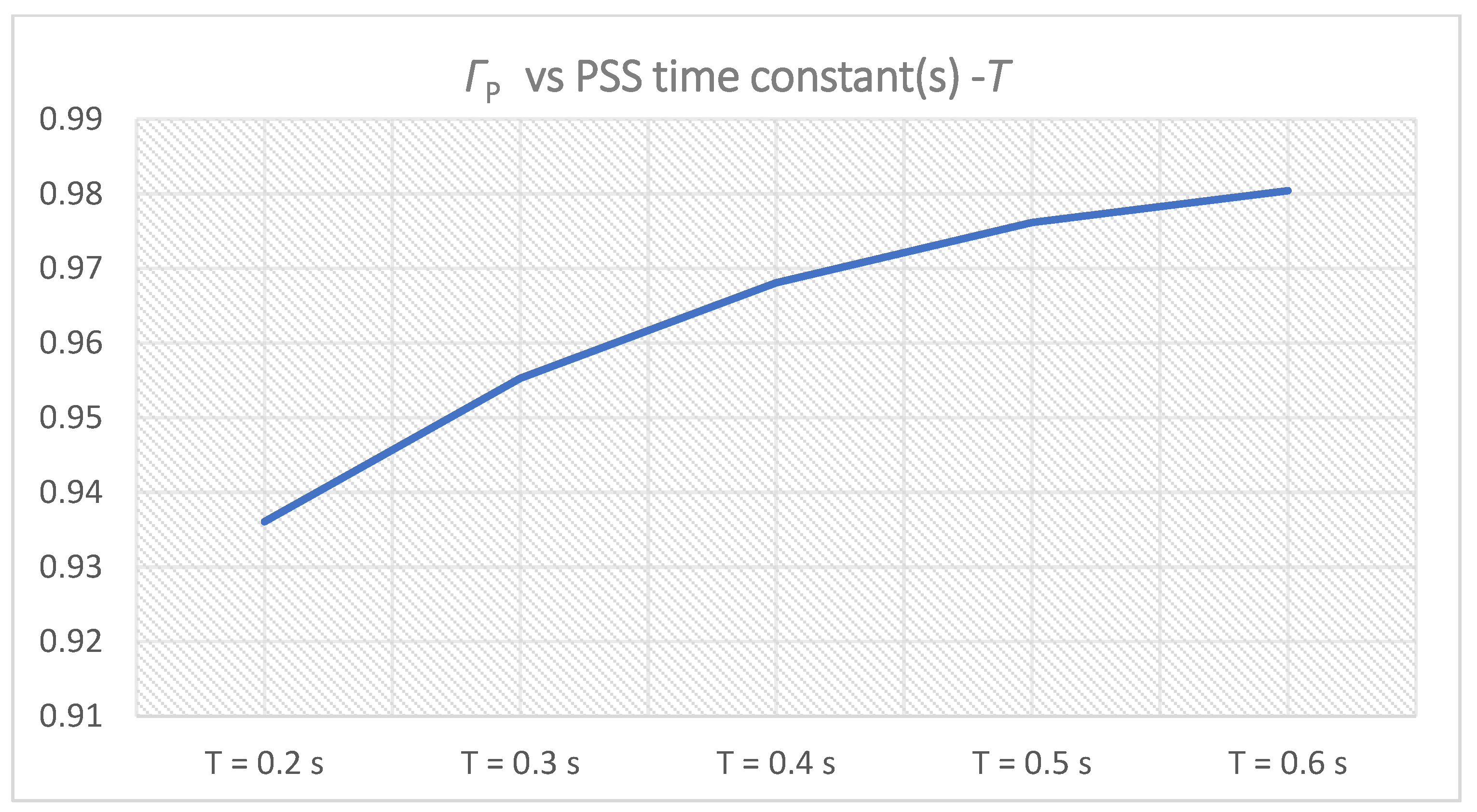
Figure 13.
ΓPi for PSS parameters K = 10, T = Ti,1 = 0.2–0.6 s.
Figure 13.
ΓPi for PSS parameters K = 10, T = Ti,1 = 0.2–0.6 s.
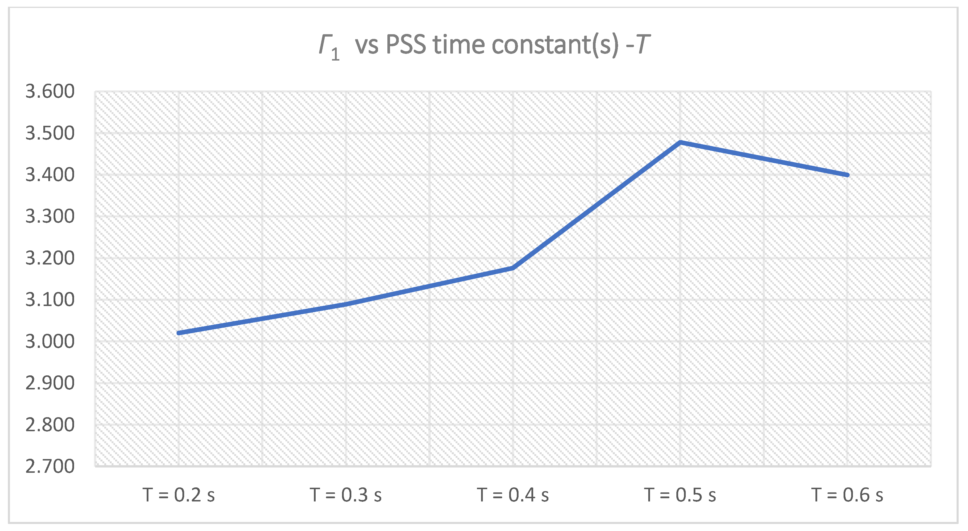
Figure 14.
Γ1 for PSS parameters K = 10, T = Ti,1 = 0.2–0.6 s.
Figure 14.
Γ1 for PSS parameters K = 10, T = Ti,1 = 0.2–0.6 s.
Figure 15.
Dominant oscillatory pole before the PSS implementation-K0,0 and after the PSS implementation with T = 0.5 s, PSS gain increase in the lower cluster 1-Ki,ln = 6–10 and the upper cluster 1 Ki,um = 10–14.
Figure 15.
Dominant oscillatory pole before the PSS implementation-K0,0 and after the PSS implementation with T = 0.5 s, PSS gain increase in the lower cluster 1-Ki,ln = 6–10 and the upper cluster 1 Ki,um = 10–14.
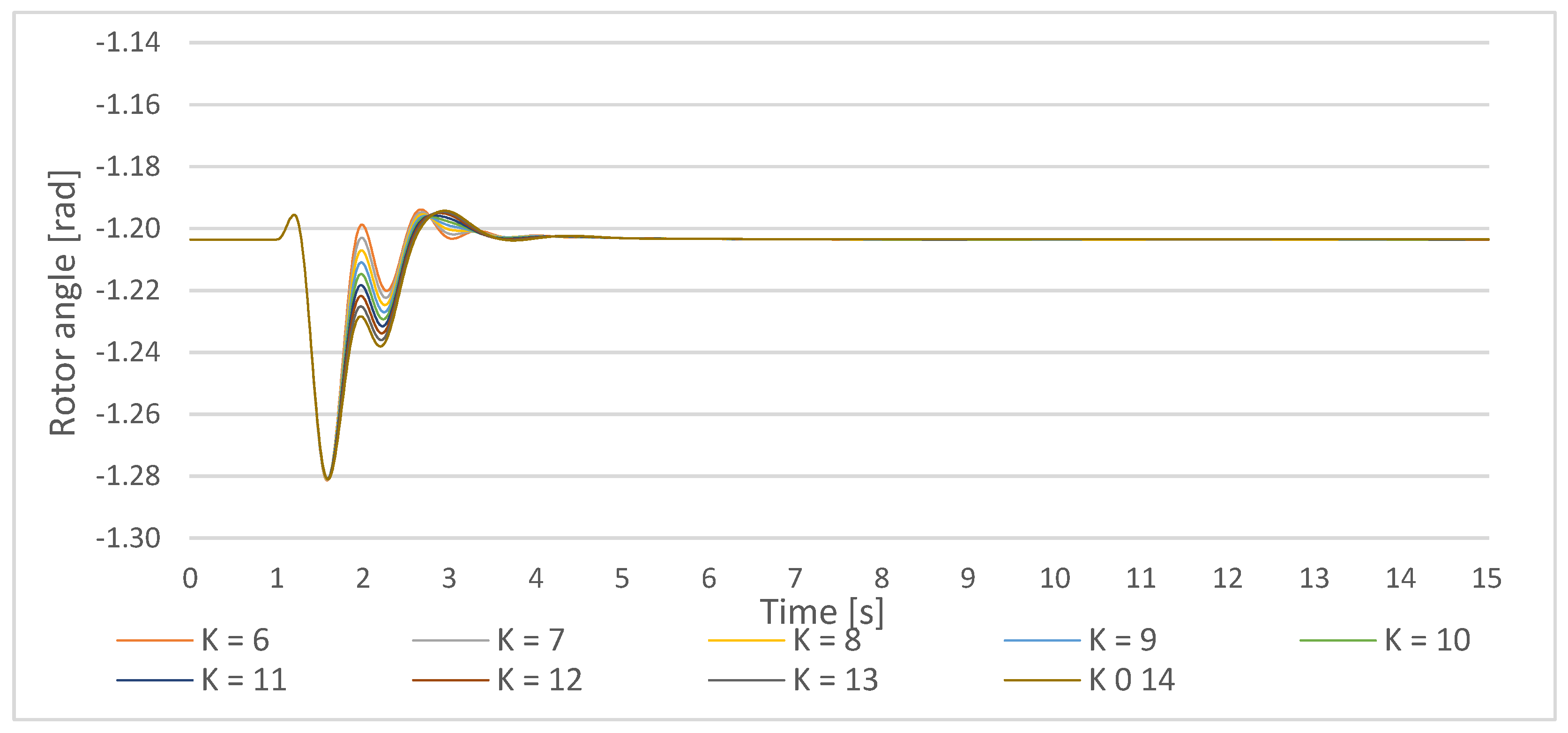
Figure 16.
Gen1 rotor angle response on a small disturbance with PSS parameters T = 0.5 s, the PSS gain increase in the lower cluster 1-Ki,ln = 6–10 and the upper cluster 1 Ki,um = 10–14.
Figure 16.
Gen1 rotor angle response on a small disturbance with PSS parameters T = 0.5 s, the PSS gain increase in the lower cluster 1-Ki,ln = 6–10 and the upper cluster 1 Ki,um = 10–14.
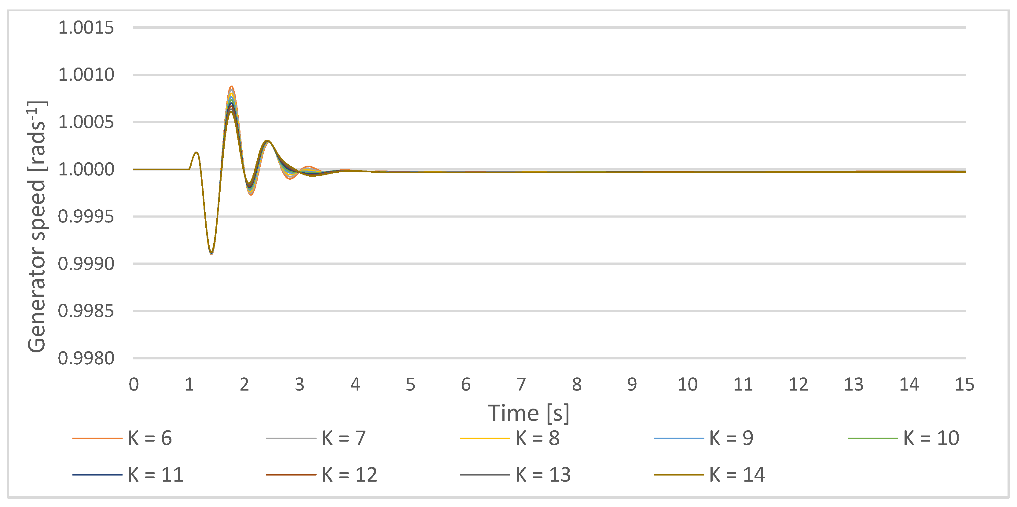
Figure 17.
Gen1 speed response on a small disturbance with PSS parameters T = 0.5 s, the PSS gain increase in the lower cluster 1-Ki,ln = 6–10, and the upper cluster 1 Ki,um = 10–14.
Figure 17.
Gen1 speed response on a small disturbance with PSS parameters T = 0.5 s, the PSS gain increase in the lower cluster 1-Ki,ln = 6–10, and the upper cluster 1 Ki,um = 10–14.
Figure 18.
Gen1 active power response on a small disturbance with PSS parameters T = 0,5 s, the PSS gain increase in the lower cluster 1-Ki,ln = 6–10 and the upper cluster 1 Ki,um = 10–14.
Figure 18.
Gen1 active power response on a small disturbance with PSS parameters T = 0,5 s, the PSS gain increase in the lower cluster 1-Ki,ln = 6–10 and the upper cluster 1 Ki,um = 10–14.
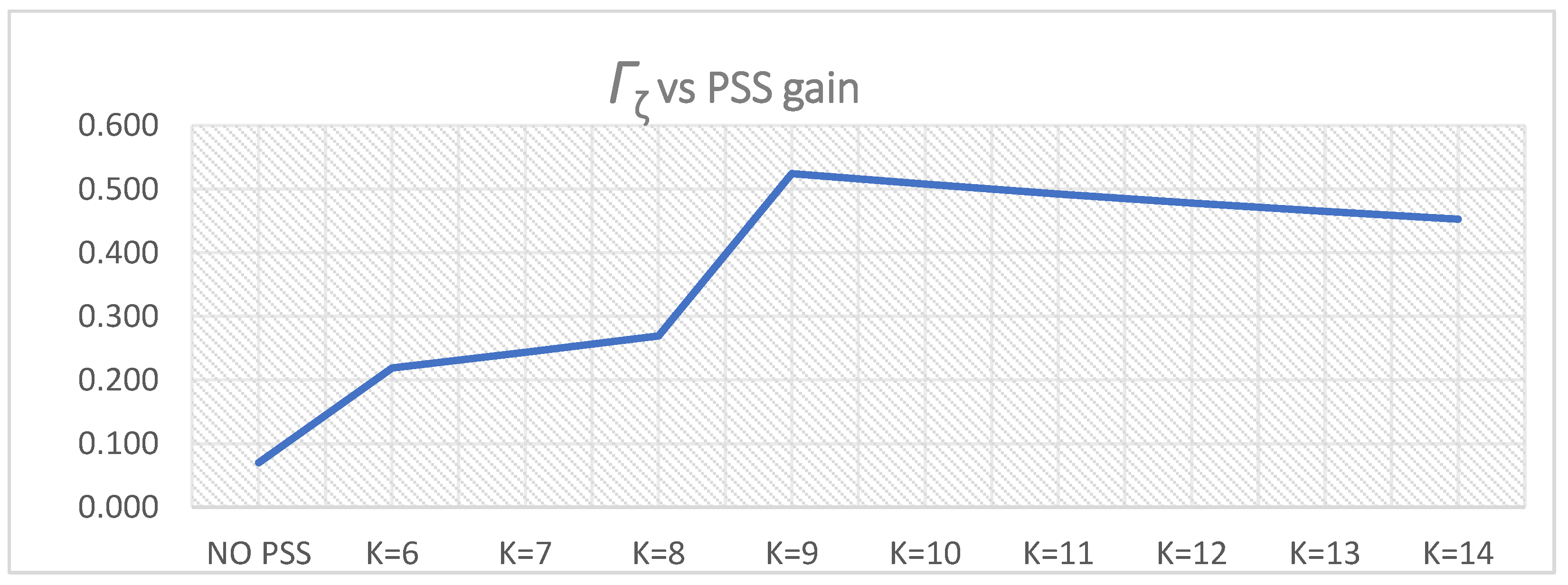
Figure 19.
Γζ (
Γζi,l1 and
Γζi,u1 from
Table 7 and
Table 8) for PSS parameters
T = 0.5 s,
K = 6–14.
Figure 19.
Γζ (
Γζi,l1 and
Γζi,u1 from
Table 7 and
Table 8) for PSS parameters
T = 0.5 s,
K = 6–14.
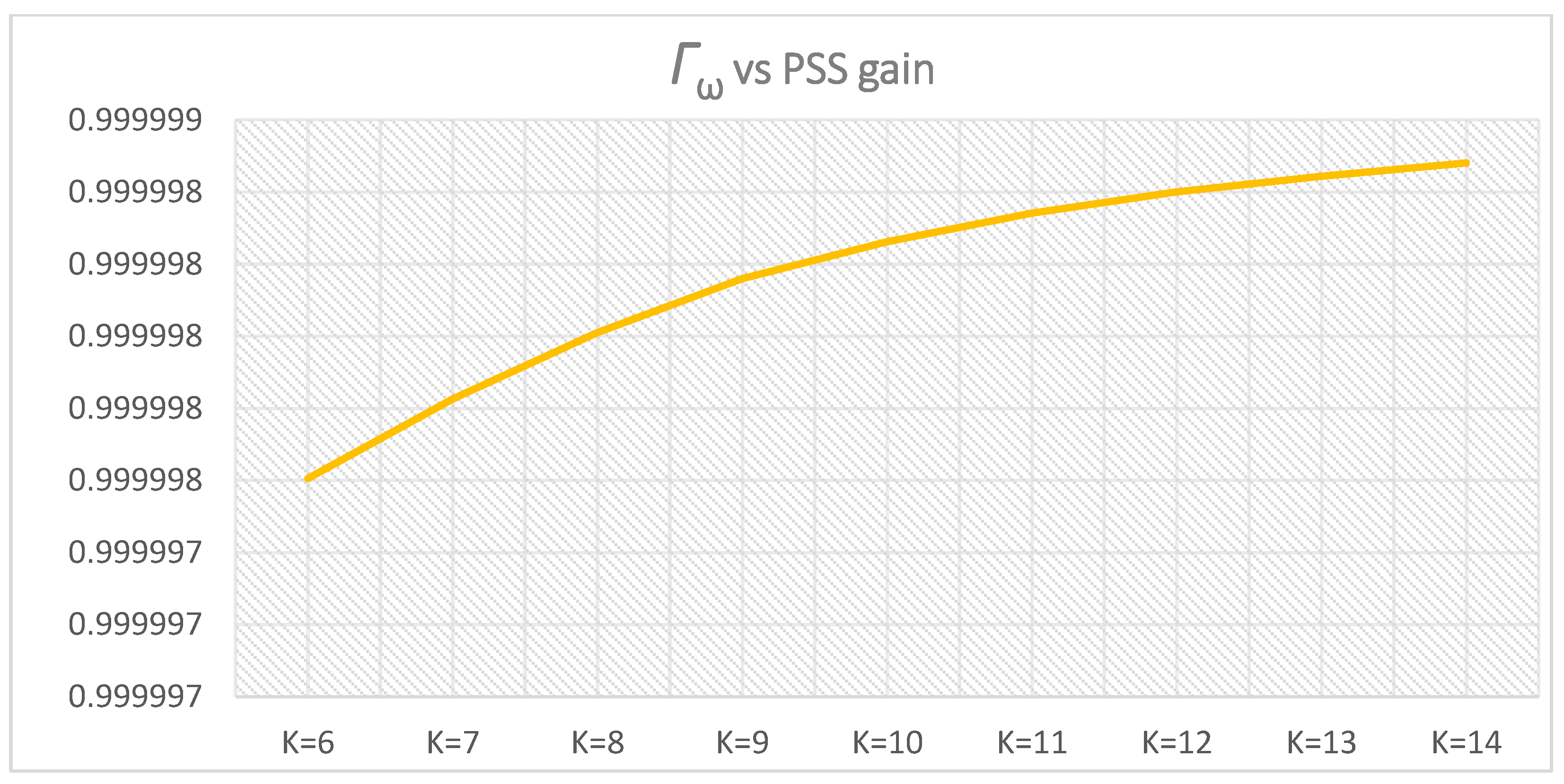
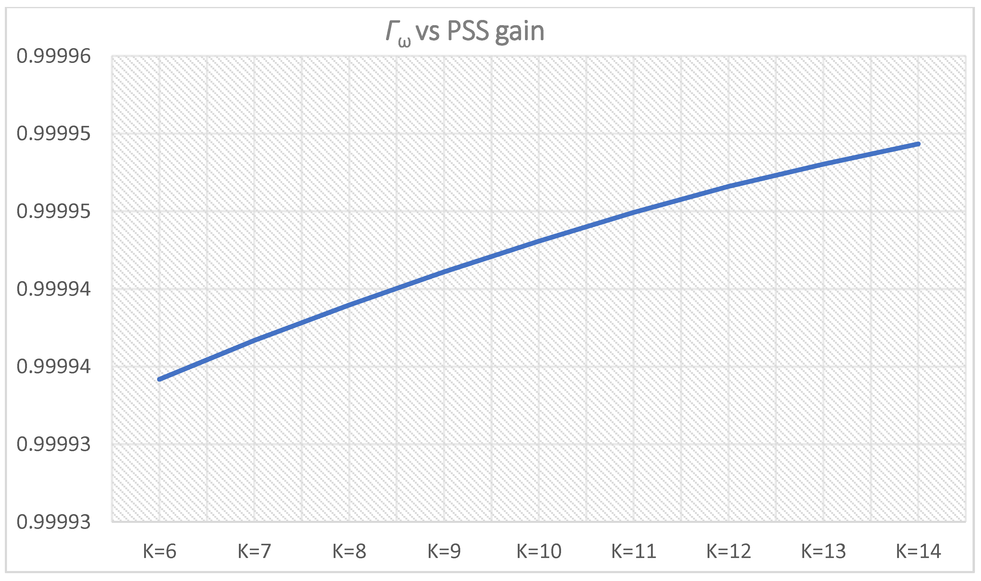
Figure 20.
Γω (
Γωi,l1 and
Γωi,u1 from
Table 7 and
Table 8) for PSS parameters
T = 0.5 s,
K = 6–14.
Figure 20.
Γω (
Γωi,l1 and
Γωi,u1 from
Table 7 and
Table 8) for PSS parameters
T = 0.5 s,
K = 6–14.
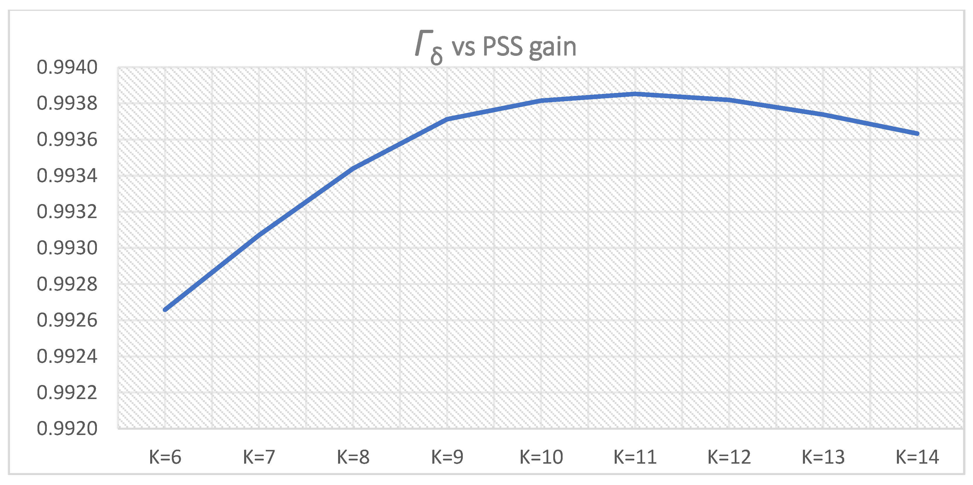
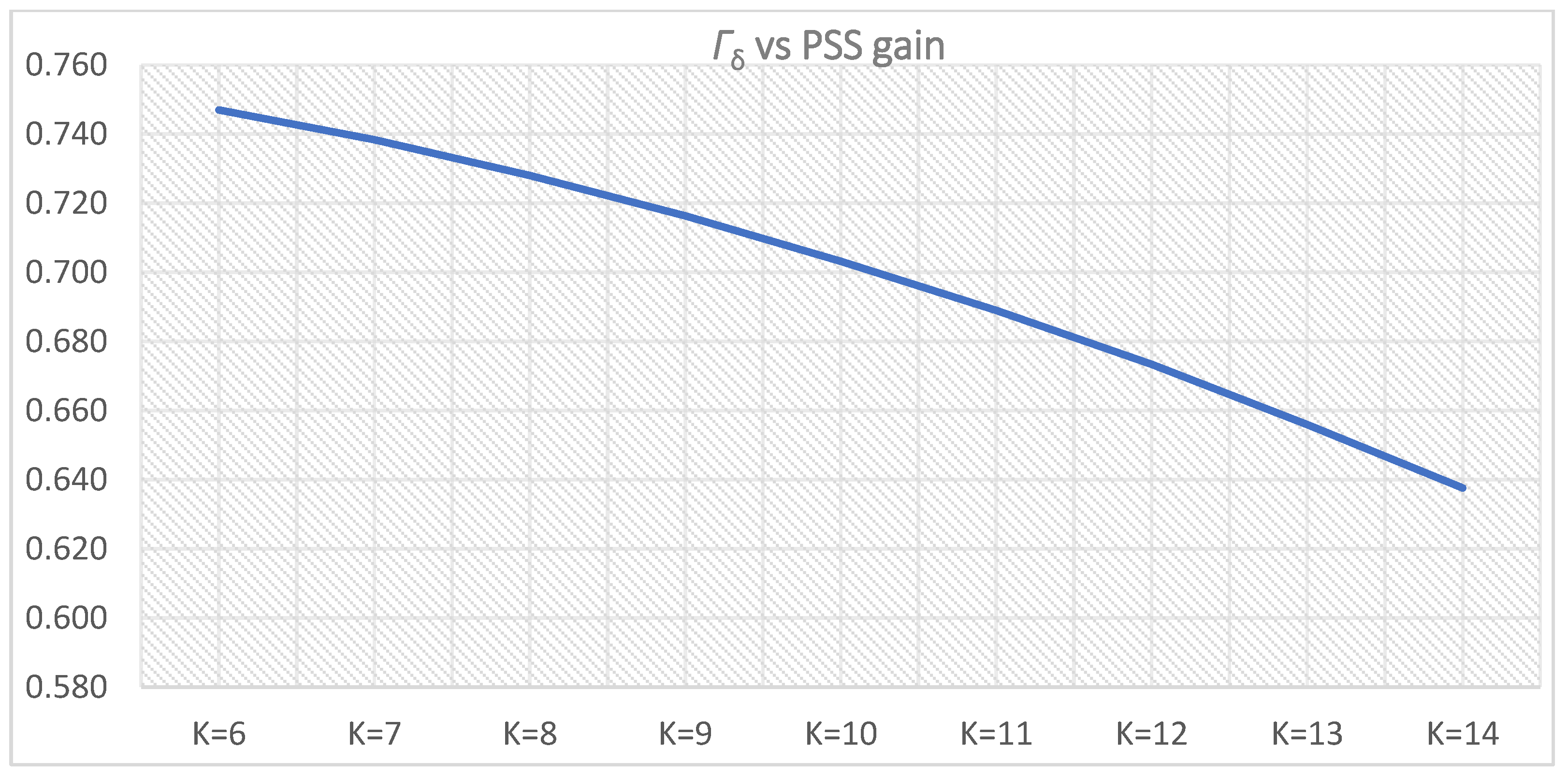
Figure 21.
Γδ (
Γδi,l1 and
Γδi,u1 from
Table 7 and
Table 8) for PSS parameters
T = 0.5 s,
K = 6–14.
Figure 21.
Γδ (
Γδi,l1 and
Γδi,u1 from
Table 7 and
Table 8) for PSS parameters
T = 0.5 s,
K = 6–14.
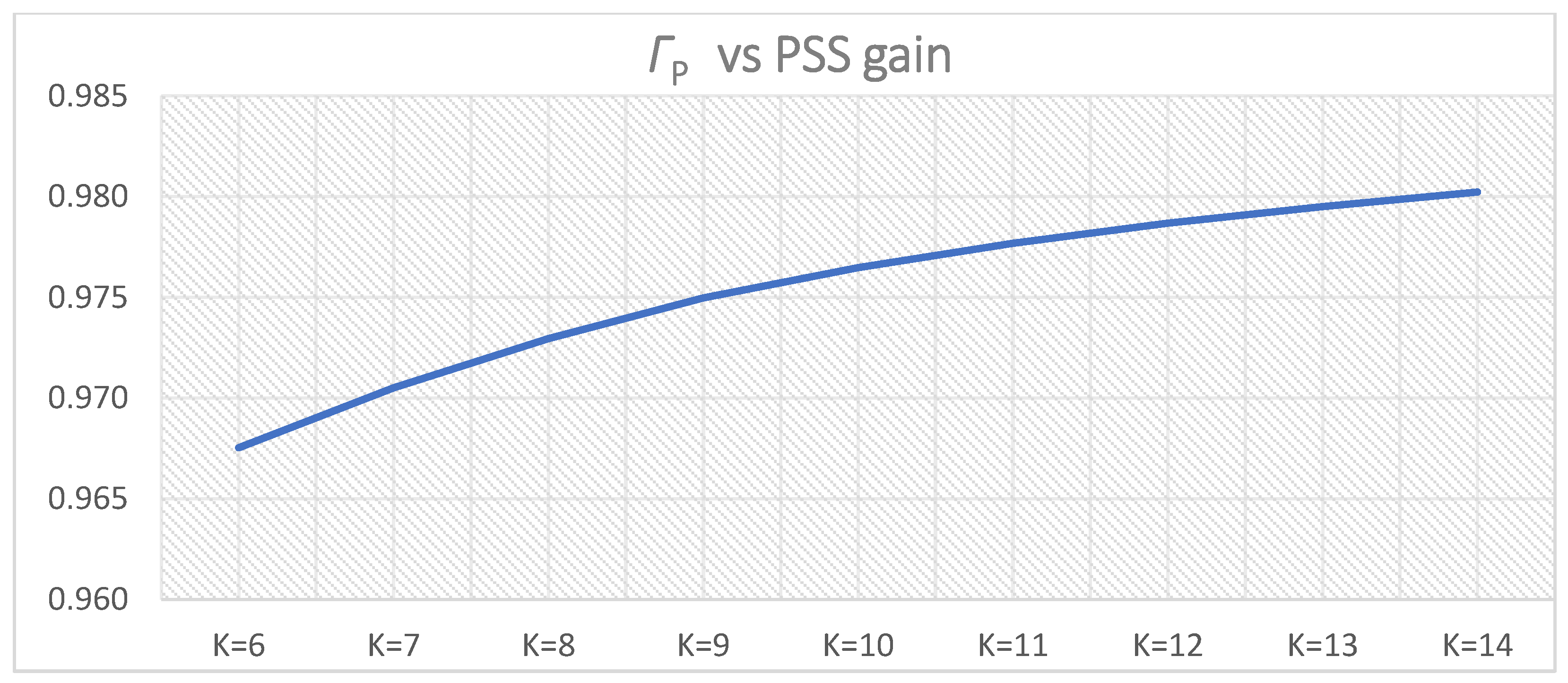
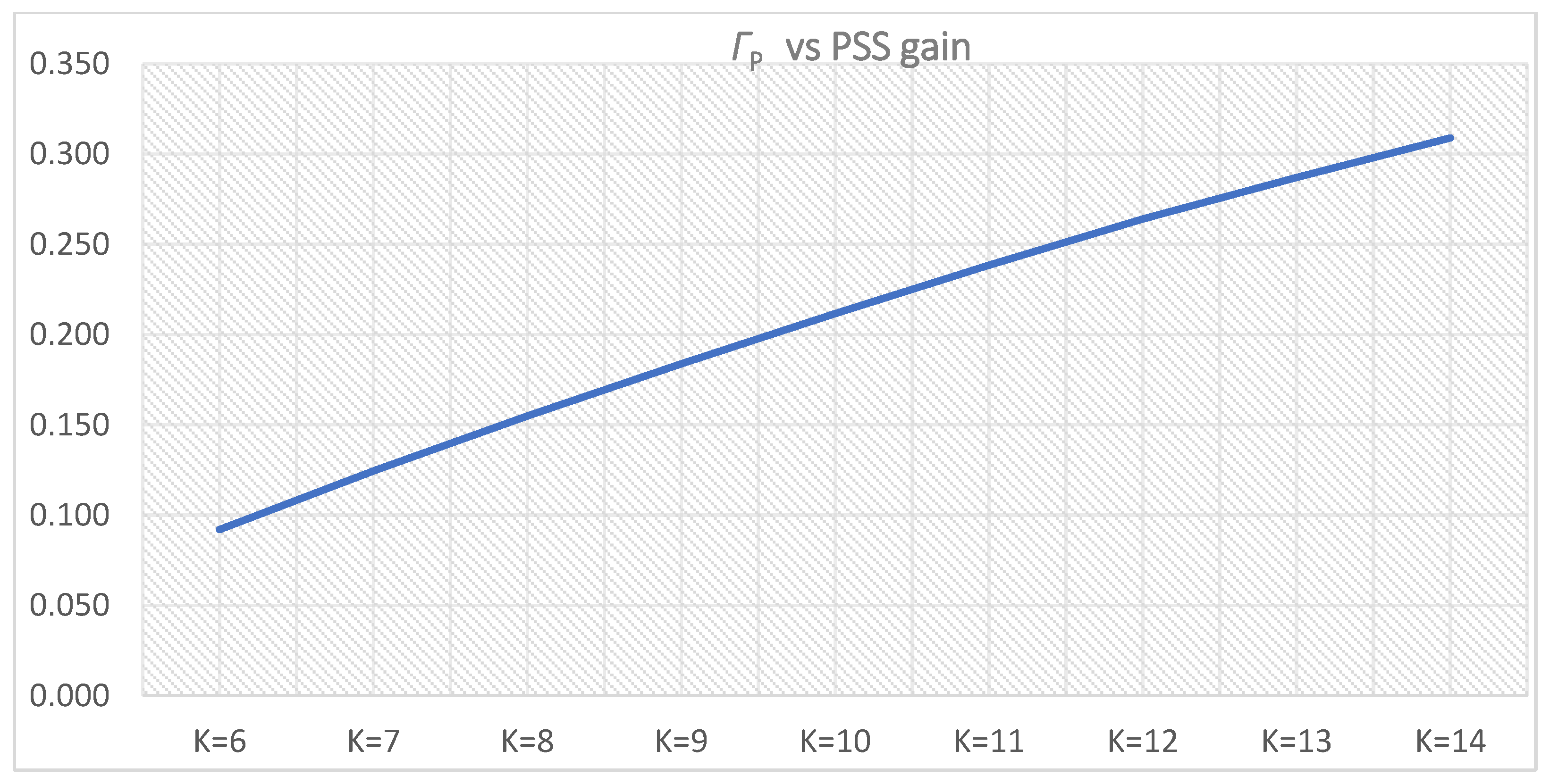
Figure 22.
ΓP (
ΓPi,l1 and
ΓPi,u1 from
Table 7 and
Table 8) for PSS parameters
T = 0.5 s,
K = 6–14.
Figure 22.
ΓP (
ΓPi,l1 and
ΓPi,u1 from
Table 7 and
Table 8) for PSS parameters
T = 0.5 s,
K = 6–14.
Figure 23.
Gen1 rotor angle response on a small disturbance with PSS parameters T = 0.5 s, the PSS gain increase in the lower cluster 1-Ki,ln = 6–10, and the upper cluster 1 Ki,um = 10–14.
Figure 23.
Gen1 rotor angle response on a small disturbance with PSS parameters T = 0.5 s, the PSS gain increase in the lower cluster 1-Ki,ln = 6–10, and the upper cluster 1 Ki,um = 10–14.
Figure 24.
Gen1 speed response on a small disturbance with PSS parameters T = 0.5 s, the PSS gain increase in the lower cluster 1-Ki,ln = 6–10, and the upper cluster 1 Ki,um = 10–14.
Figure 24.
Gen1 speed response on a small disturbance with PSS parameters T = 0.5 s, the PSS gain increase in the lower cluster 1-Ki,ln = 6–10, and the upper cluster 1 Ki,um = 10–14.
Figure 25.
Gen1 active power response on a small disturbance with PSS parameters T = 0.5 s, the PSS gain increase in the lower cluster 1-Ki,ln = 6–10, and the upper cluster 1 Ki,um = 10–14.
Figure 25.
Gen1 active power response on a small disturbance with PSS parameters T = 0.5 s, the PSS gain increase in the lower cluster 1-Ki,ln = 6–10, and the upper cluster 1 Ki,um = 10–14.
Figure 26.
Γζ (
Γζi,l1 and
Γζi,u1 from
Table 9 and
Table 10) for PSS parameters
T = 0.5 s,
K = 6–14.
Figure 26.
Γζ (
Γζi,l1 and
Γζi,u1 from
Table 9 and
Table 10) for PSS parameters
T = 0.5 s,
K = 6–14.
Figure 27.
Γω (
Γωi,l1 and
Γωi,u1 from
Table 9 and
Table 10) for PSS parameters
T = 0.5 s,
K = 6–14.
Figure 27.
Γω (
Γωi,l1 and
Γωi,u1 from
Table 9 and
Table 10) for PSS parameters
T = 0.5 s,
K = 6–14.
Figure 28.
Γδ (
Γδi,l1 and
Γδi,u1 from
Table 9 and
Table 10) for PSS parameters
T = 0.5 s,
K = 6–14.
Figure 28.
Γδ (
Γδi,l1 and
Γδi,u1 from
Table 9 and
Table 10) for PSS parameters
T = 0.5 s,
K = 6–14.
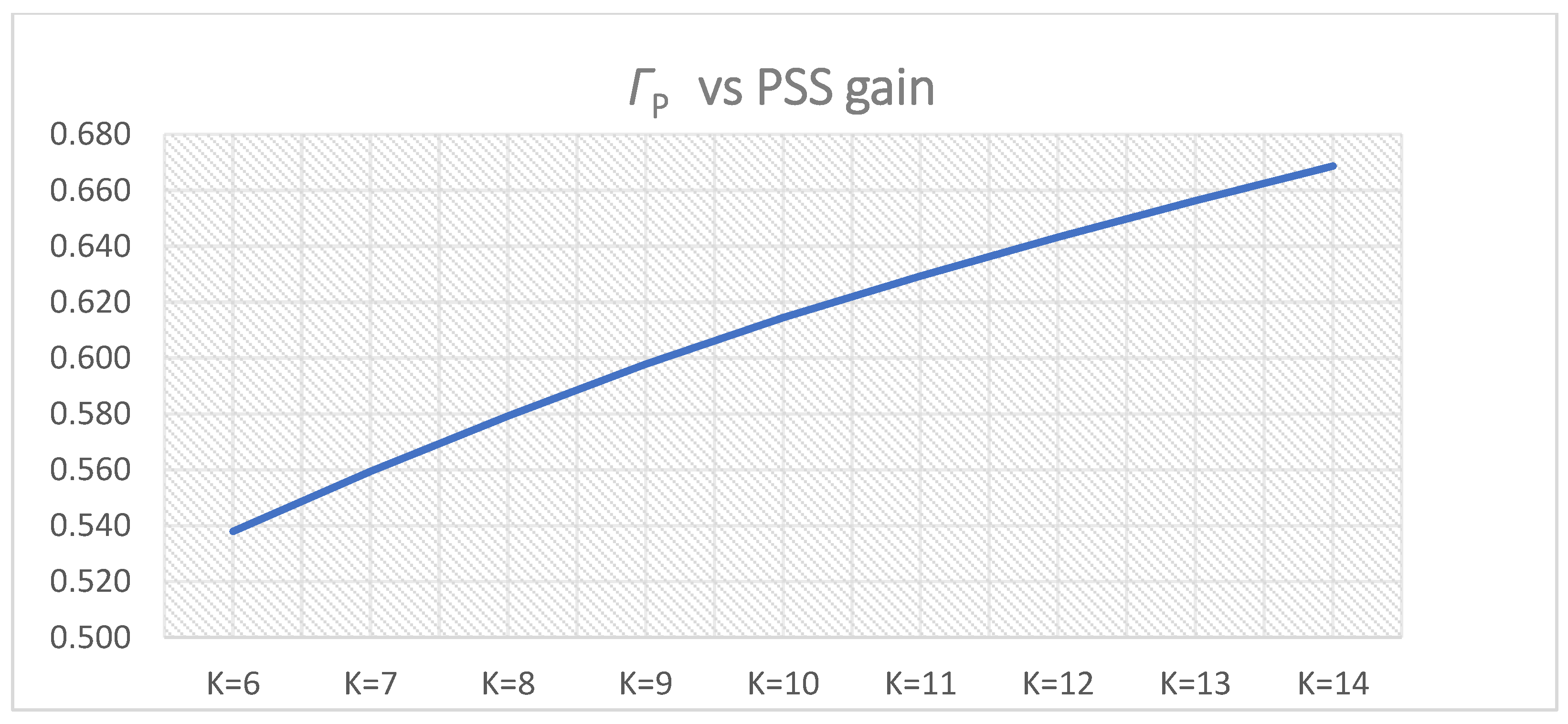
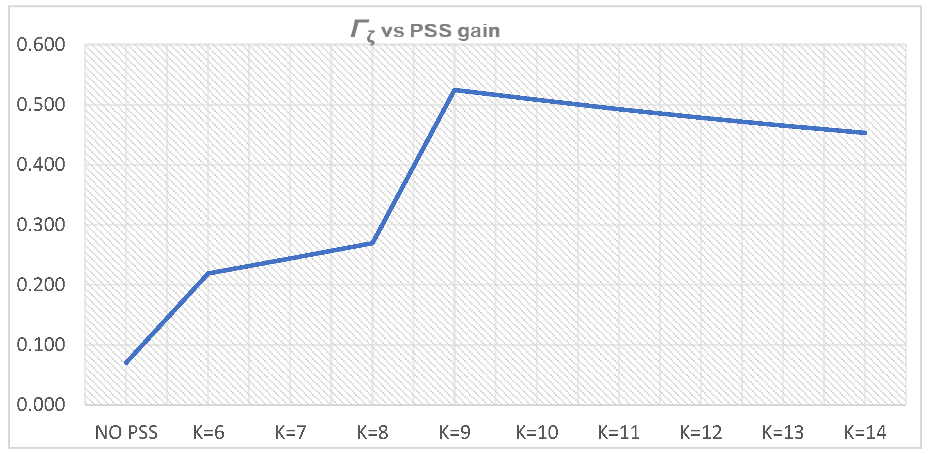
Figure 29.
ΓP (
ΓPi,l1 and
ΓPi,u1 from
Table 9 and
Table 10) for PSS parameters
T = 0.5 s,
K = 6–14.
Figure 29.
ΓP (
ΓPi,l1 and
ΓPi,u1 from
Table 9 and
Table 10) for PSS parameters
T = 0.5 s,
K = 6–14.
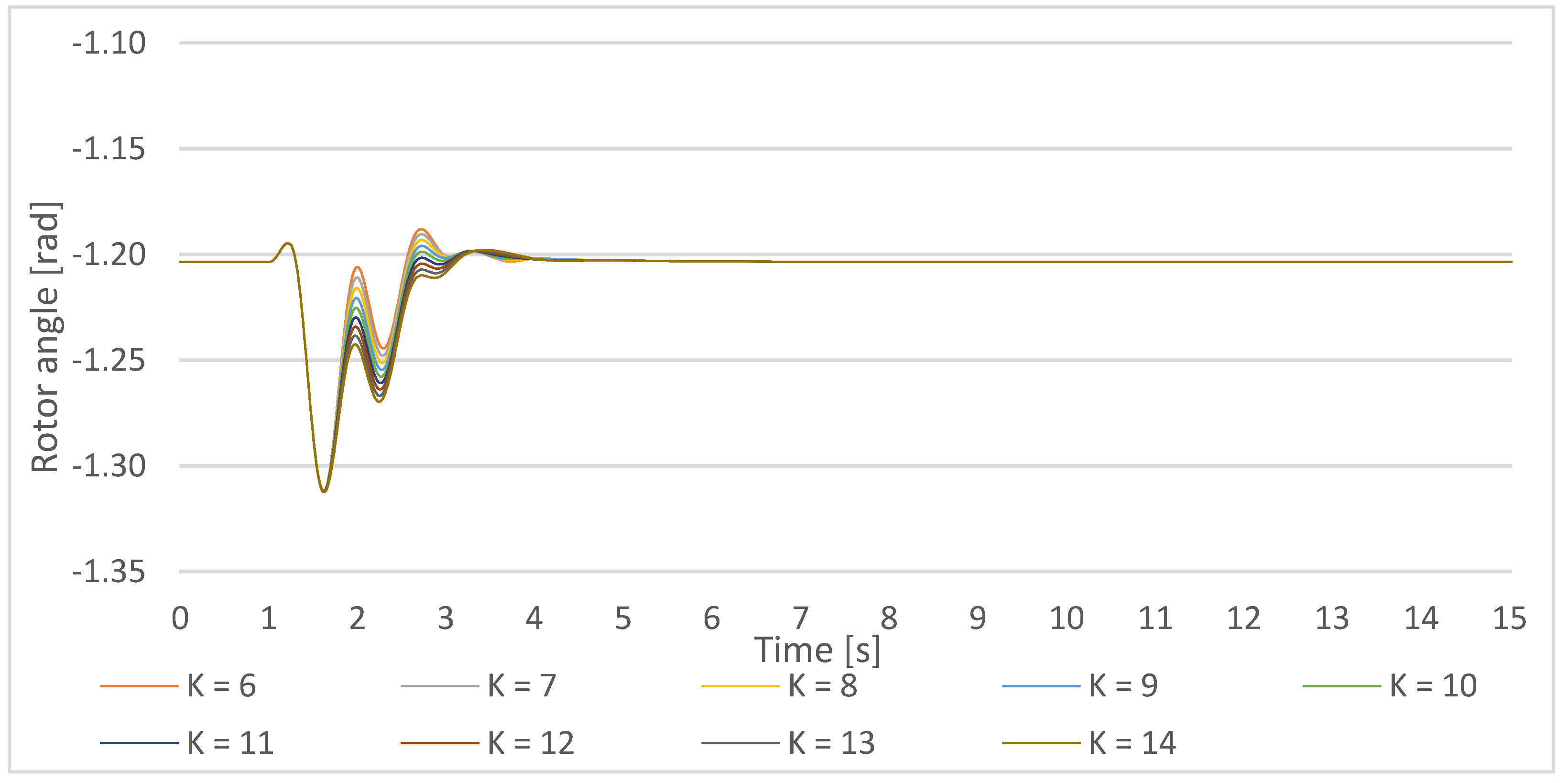
Figure 30.
Gen1 rotor angle response on a small disturbance with PSS parameters T = 0.5 s, the PSS gain increase in the lower cluster 1-Ki,ln = 6–10, and the upper cluster 1 Ki,um = 10–14.
Figure 30.
Gen1 rotor angle response on a small disturbance with PSS parameters T = 0.5 s, the PSS gain increase in the lower cluster 1-Ki,ln = 6–10, and the upper cluster 1 Ki,um = 10–14.
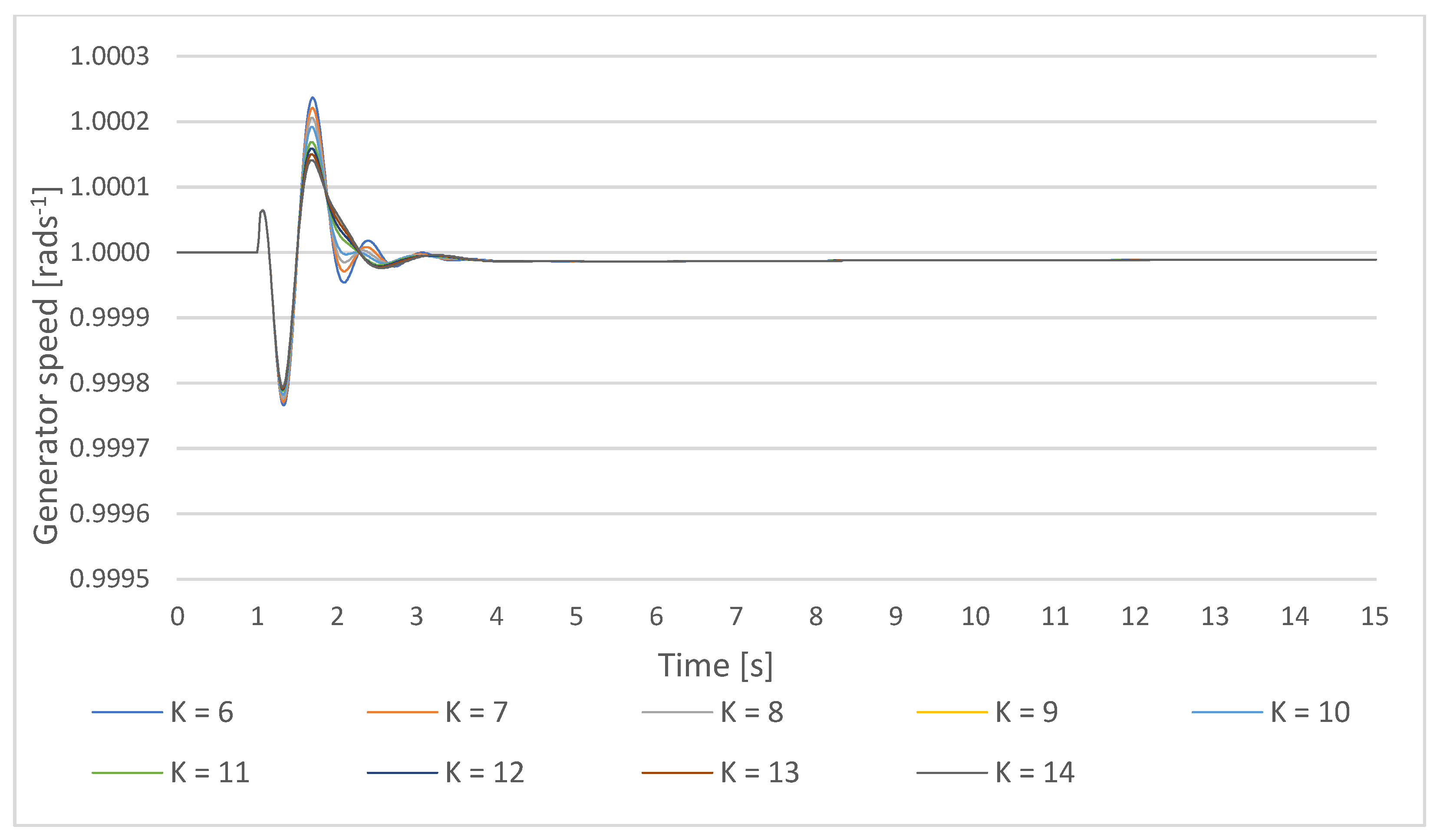
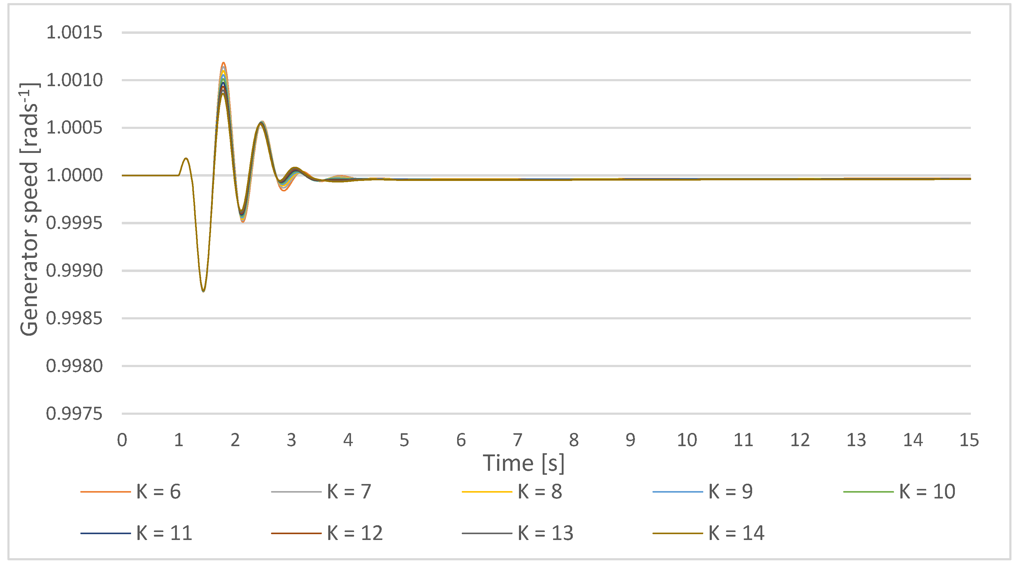
Figure 31.
Gen1 speed response on a small disturbance with PSS parameters T = 0.5 s, the PSS gain increase in the lower cluster 1-Ki,ln = 6–10, and the upper cluster 1 Ki,um = 10–14.
Figure 31.
Gen1 speed response on a small disturbance with PSS parameters T = 0.5 s, the PSS gain increase in the lower cluster 1-Ki,ln = 6–10, and the upper cluster 1 Ki,um = 10–14.
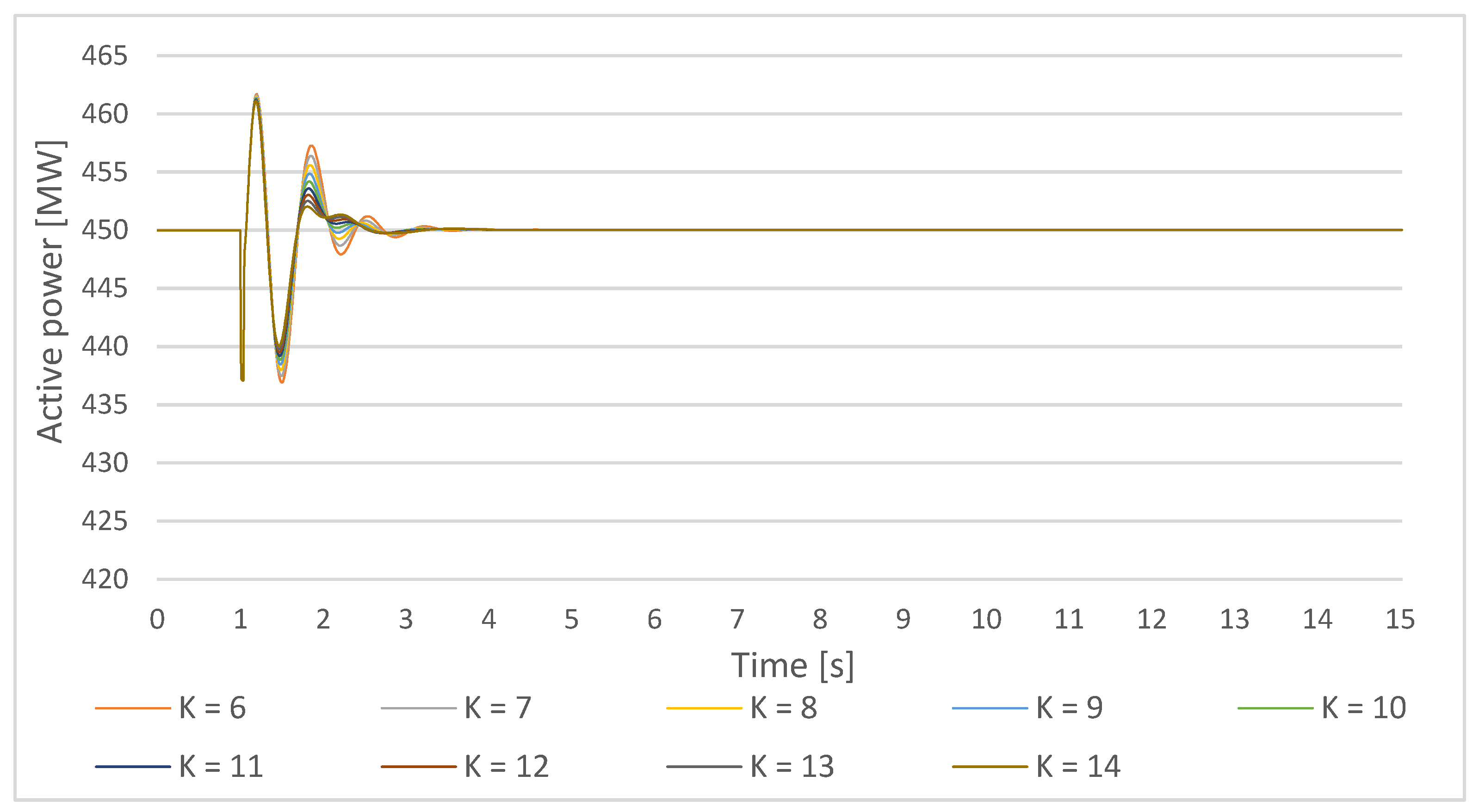
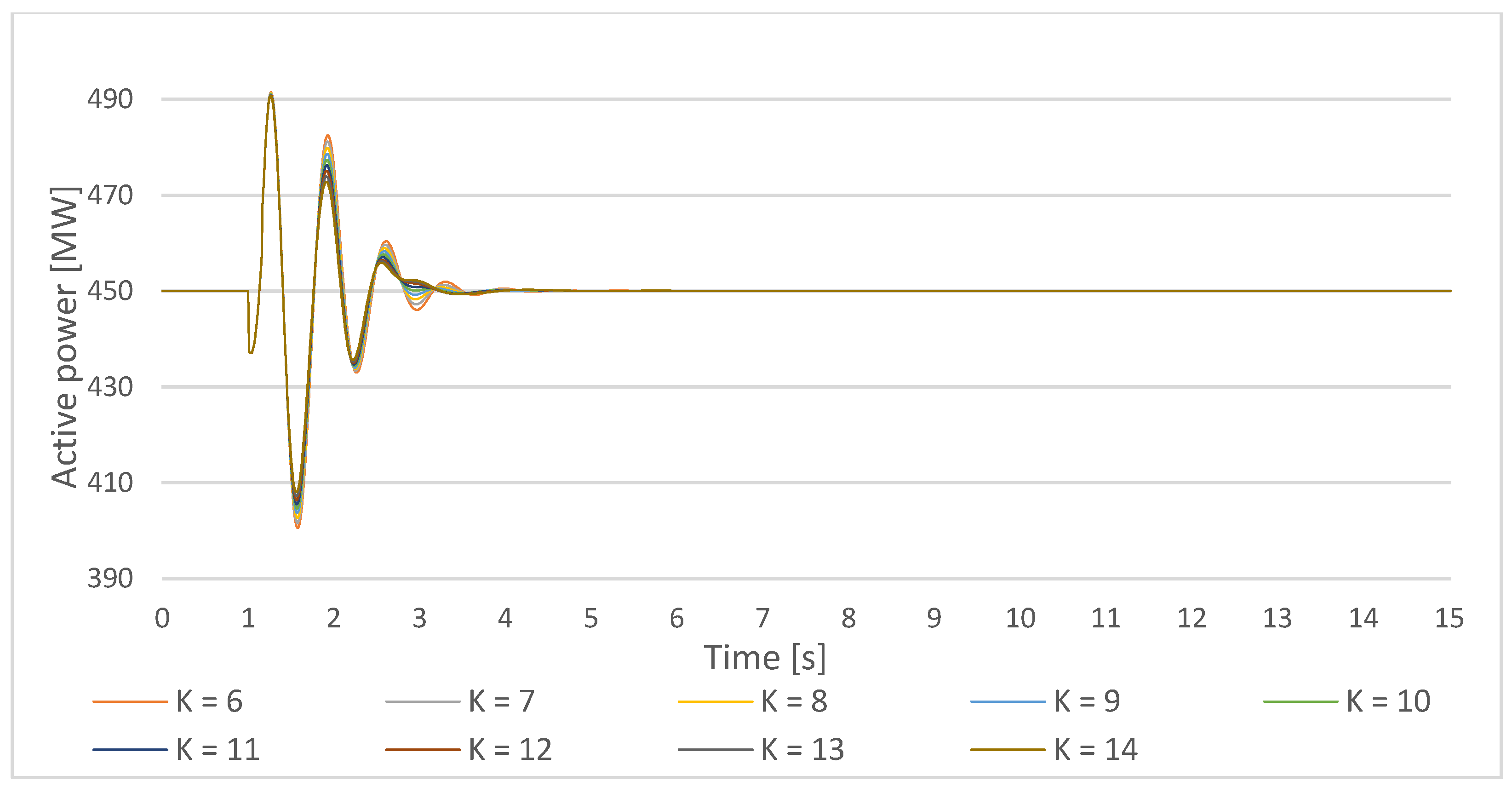
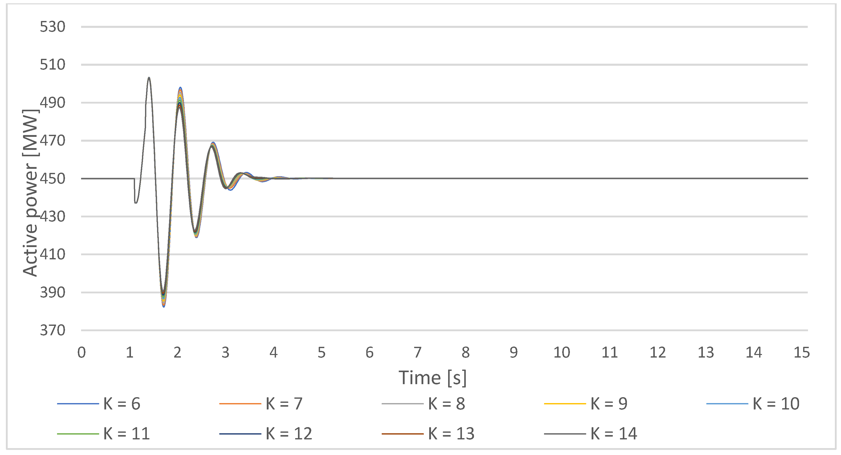
Figure 32.
Gen1 active power response on a small disturbance with PSS parameters T = 0.5 s, the PSS gain increase in the lower cluster 1-Ki,ln = 6–10, and the upper cluster 1 Ki,um = 10–14.
Figure 32.
Gen1 active power response on a small disturbance with PSS parameters T = 0.5 s, the PSS gain increase in the lower cluster 1-Ki,ln = 6–10, and the upper cluster 1 Ki,um = 10–14.
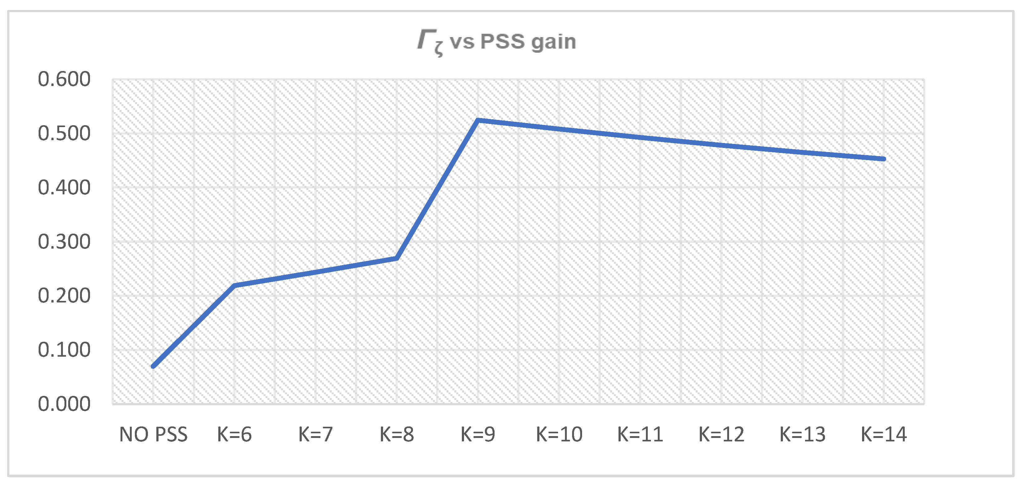
Figure 33.
Γζ (
Γζi,l1 and
Γζi,u1 from
Table 11 and
Table 12) for PSS parameters
T = 0.5 s,
K = 6–14.
Figure 33.
Γζ (
Γζi,l1 and
Γζi,u1 from
Table 11 and
Table 12) for PSS parameters
T = 0.5 s,
K = 6–14.
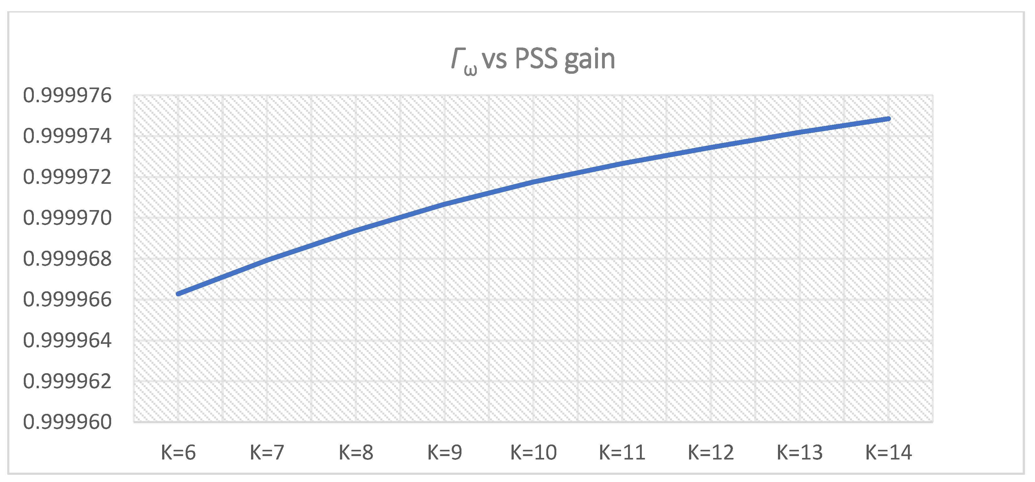
Figure 34.
Γω (
Γωi,l1 and
Γωi,u1 from
Table 11 and
Table 12) for PSS parameters
T = 0.5 s,
K = 6–14.
Figure 34.
Γω (
Γωi,l1 and
Γωi,u1 from
Table 11 and
Table 12) for PSS parameters
T = 0.5 s,
K = 6–14.
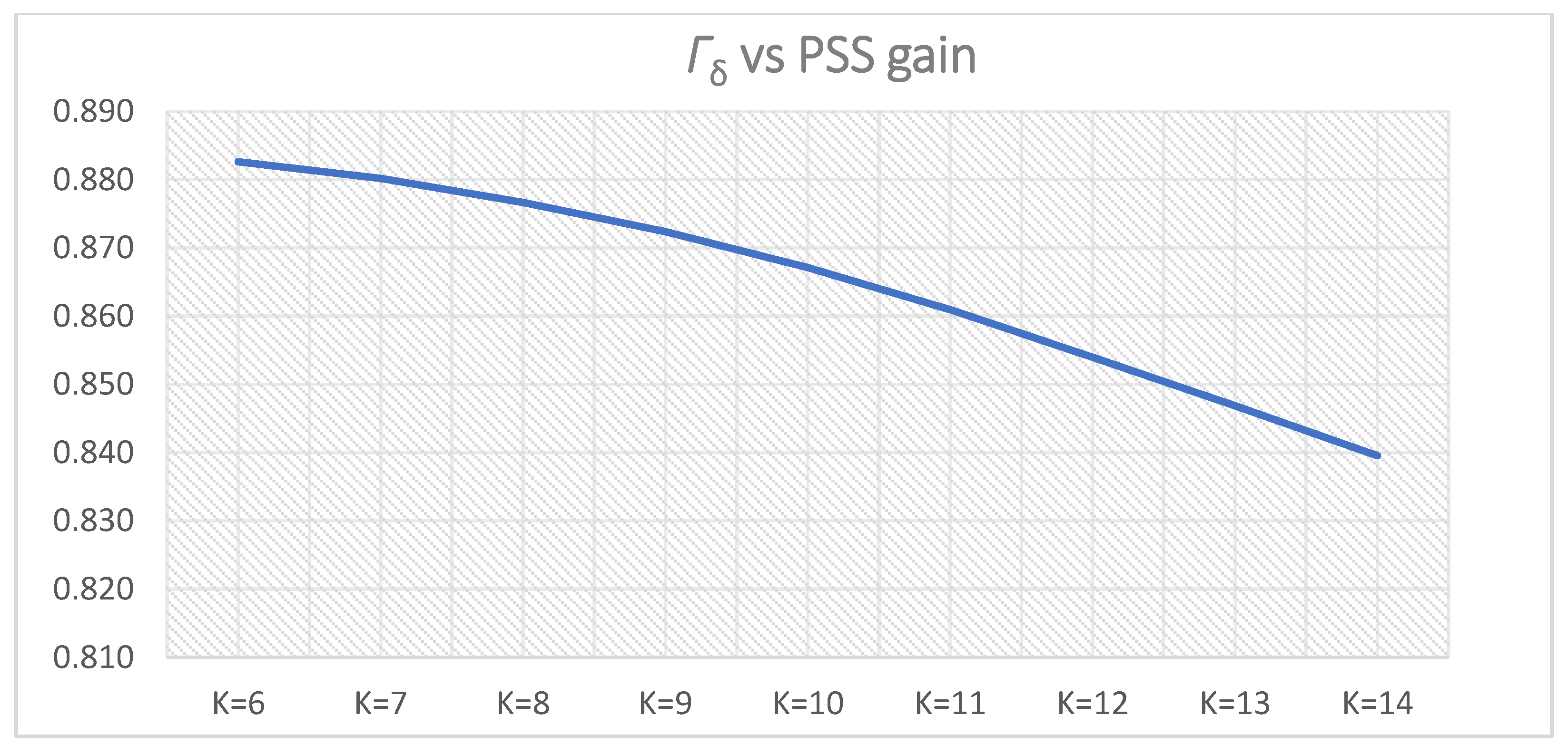
Figure 35.
Γδ (
Γδi,l1 and
Γδi,u1 from
Table 11 and
Table 12) for PSS parameters
T = 0.5 s,
K = 6–14.
Figure 35.
Γδ (
Γδi,l1 and
Γδi,u1 from
Table 11 and
Table 12) for PSS parameters
T = 0.5 s,
K = 6–14.
Figure 36.
ΓP (
ΓPi,l1 and
ΓPi,u1 from
Table 11 and
Table 12) for PSS parameters
T = 0.5 s,
K = 6–14.
Figure 36.
ΓP (
ΓPi,l1 and
ΓPi,u1 from
Table 11 and
Table 12) for PSS parameters
T = 0.5 s,
K = 6–14.
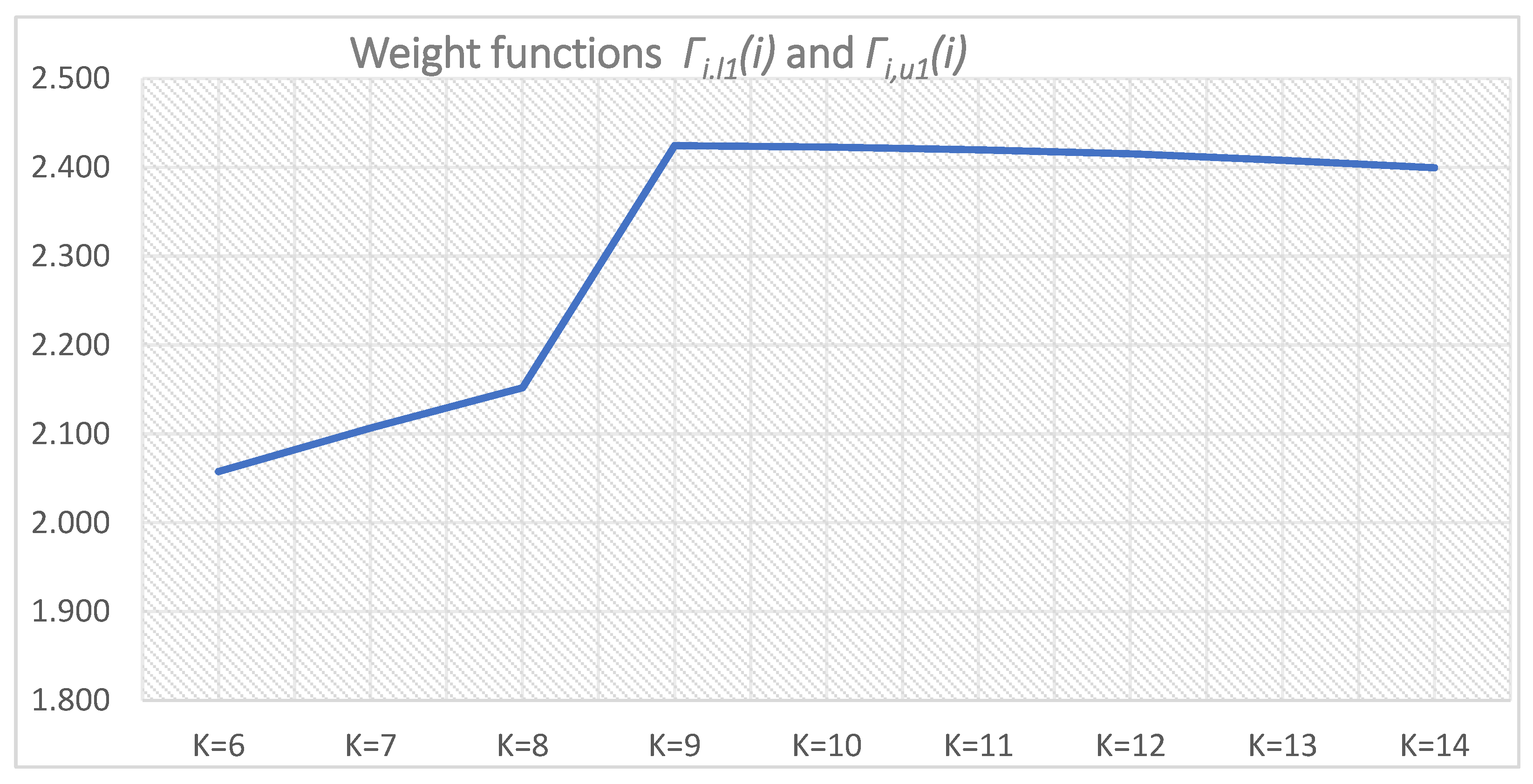
Figure 37.
Weight functions: Γi,l1(i)—(i = 0–4 for K = 6–10), Γi,u1(i) (i = 0–4 for K = 10–14), T = 0.5 s.
Figure 37.
Weight functions: Γi,l1(i)—(i = 0–4 for K = 6–10), Γi,u1(i) (i = 0–4 for K = 10–14), T = 0.5 s.
Table 1.
Local oscillatory modes for the analyzed system without the PSS implementation.
Table 1.
Local oscillatory modes for the analyzed system without the PSS implementation.
| Mode Number | α [s−1] | ±jω [rad s−1] | Ξ |
|---|
| Mode 1 | −0.6029112884 | 8.6001286177 | 0.069933275444 |
| Mode 2 | −3.0888275889 | 9.1371914398 | 0.32024636109 |
| Mode 3 | −3.3668021306 | 10.953437301 | 0.30026554697 |
| Mode 4 | −3.7886935644 | 11.819709815 | 0.30524242934 |
| Mode 5 | −4.5222909467 | 12.584279377 | 0.33818650996 |
Table 2.
Participation of the generator speed state variable for the dominant oscillatory mode.
Table 2.
Participation of the generator speed state variable for the dominant oscillatory mode.
| Generator Unit | Participation in Mode 1 |
|---|
| Gen1 | 0.954 |
| Gen2 | 0.120 |
| Gen3 | 0.005 |
| Gen4 | 0.003 |
| Gen5 | 0.002 |
| External Grid | 0.046 |
Table 3.
Dominant oscillatory pole for PSS parameters K = 10, T = Ti,1 = 0.2–0.6 s (cluster 1).
Table 3.
Dominant oscillatory pole for PSS parameters K = 10, T = Ti,1 = 0.2–0.6 s (cluster 1).
| i | Ti,1 [s] | α [s−1] | ±jω [rad s−1] | ξ |
|---|
| 0 | 0.2 | −0.846729311 | 8.6001286177 | 0.094299372 |
| 1 | 0.3 | −1.306793920 | 9.1371914398 | 0.141835333 |
| 2 | 0.4 | −2.059476510 | 10.953437301 | 0.214871539 |
| 3 | 0.5 | −2.442664922 | 11.819709815 | 0.507928180 |
| 4 | 0.6 | −2.024097138 | 12.584279377 | 0.425562142 |
Table 4.
Weight functions for K = 10, T = Ti,1 = 0.2–0.6 s (cluster 1).
Table 4.
Weight functions for K = 10, T = Ti,1 = 0.2–0.6 s (cluster 1).
| i | Ti,1 [s] | Γζi | Γωi | Γδi | ΓPi | Γ1(i)
|
|---|
| 0 | 0.2 | 0.094299 | 0.999995596 | 0.989720196 | 0.936069374 | 3.02008453797 |
| 1 | 0.3 | 0.141835 | 0.999996902 | 0.991708475 | 0.955296445 | 3.08883715433 |
| 2 | 0.4 | 0.214872 | 0.999997748 | 0.993060487 | 0.968084688 | 3.17601446330 |
| 3 | 0.5 | 0.507928 | 0.999998262 | 0.993814845 | 0.976163024 | 3.47790431049 |
| 4 | 0.6 | 0.425562 | 0.999998447 | 0.993415907 | 0.980405629 | 3.39938212468 |
Table 5.
Dominant oscillatory pole for PSS parameters T = T1 = T3 = 0.5 s, Ki,ln = 6–10, n = 1 (lower cluster 1).
Table 5.
Dominant oscillatory pole for PSS parameters T = T1 = T3 = 0.5 s, Ki,ln = 6–10, n = 1 (lower cluster 1).
| i | Ki,l1 | α [s−1] | ±jω [rad s−1] | ξ |
|---|
| | NO PSS | −0.602911288 | ±8.600128618 | 0.069933275 |
| 0 | 6 | −2.044897210 | ±9.123657619 | 0.218705293 |
| 1 | 7 | −2.323979821 | ±9.251852650 | 0.243622413 |
| 2 | 8 | −2.615513529 | ±9.361915009 | 0.269074414 |
| 3 | 9 | −2.536071719 | ±4.118411476 | 0.524347042 |
| 4 | 10 | −2.442664922 | ±4.142534779 | 0.50792818 |
Table 6.
Dominant oscillatory pole for PSS parameters T = 0.5 s, Ki,um = 10–14, m = 1 (upper cluster 1).
Table 6.
Dominant oscillatory pole for PSS parameters T = 0.5 s, Ki,um = 10–14, m = 1 (upper cluster 1).
| i | Ki,u1 | α [s−1] | ±jω [rad s−1] | ξ |
|---|
| 0 | 10 | −2.442664922 | ±4.142534779 | 0.50792818 |
| 1 | 11 | −2.350630618 | ±4.154693103 | 0.492426473 |
| 2 | 12 | −2.262346344 | ±4.156618791 | 0.478053895 |
| 3 | 13 | −2.179202113 | ±4.150363212 | 0.464877617 |
| 4 | 14 | −2.101785372 | ±4.137873414 | 0.452866896 |
Table 7.
Weight functions for PSS parameters T = 0.5 s, Ki,ln = 6–10, n = 1 (lower cluster 1), t = 30 ms.
Table 7.
Weight functions for PSS parameters T = 0.5 s, Ki,ln = 6–10, n = 1 (lower cluster 1), t = 30 ms.
| i | Ki,l1 | Γζi,l1 | Γωi,l1 | Γδi,l1 | ΓPi,l1 | Γi,l1(i) |
|---|
| 0 | 10 | 0.507928 | 0.9999982622 | 0.9938148445 | 0.9764722440 | 3.8037042787 |
| 1 | 9 | 0.524347 | 0.9999981598 | 0.9937118105 | 0.9749639780 | 3.8180089833 |
| 2 | 8 | 0.269074 | 0.9999980102 | 0.9934398148 | 0.9729530840 | 3.5597830173 |
| 3 | 7 | 0.243622 | 0.9999978261 | 0.9930707387 | 0.9705117330 | 3.5307066213 |
| 4 | 6 | 0.218705 | 0.9999976055 | 0.9926580155 | 0.9675305460 | 3.5014016407 |
Table 8.
Weight functions for PSS parameters T = 0.5 s, Ki,um = 10–14, m = 1 (upper cluster 1); t = 30 ms.
Table 8.
Weight functions for PSS parameters T = 0.5 s, Ki,um = 10–14, m = 1 (upper cluster 1); t = 30 ms.
| i | Ki,u1 | Γζi,u1 | Γωi,u1 | Γδi,u1 | ΓPi,u1 | Γi,u1(i) |
|---|
| 0 | 10 | 0.507928 | 0.9999982622 | 0.9938148445 | 0.976472244 | 3.80370427871 |
| 1 | 11 | 0.492426 | 0.9999983415 | 0.9938523457 | 0.977678002 | 3.78984782950 |
| 2 | 12 | 0.478054 | 0.9999984003 | 0.9938187092 | 0.978677412 | 3.77677422066 |
| 3 | 13 | 0.464878 | 0.9999984437 | 0.9937383989 | 0.979498216 | 3.76461208143 |
| 4 | 14 | 0.452867 | 0.9999984808 | 0.9936327709 | 0.980223698 | 3.75346307772 |
Table 9.
Weight functions for PSS parameters T = 0.5 s, Ki,ln = 6–10, n = 1 (lower cluster 1), t = 150 ms.
Table 9.
Weight functions for PSS parameters T = 0.5 s, Ki,ln = 6–10, n = 1 (lower cluster 1), t = 150 ms.
| i | Ki,l1 | Γζi,l1 | Γωi,l1 | Γδi,l1 | ΓPi,l1 | Γi,l1(i) |
|---|
| 0 | 10 | 0.507928 | 0.9999717530 | 0.8671126304 | 0.6144343930 | 2.9894469569 |
| 1 | 9 | 0.524347 | 0.9999706671 | 0.8723687207 | 0.5977923551 | 2.9944787854 |
| 2 | 8 | 0.269074 | 0.9999693749 | 0.8766792552 | 0.5791968020 | 2.7249198464 |
| 3 | 7 | 0.243622 | 0.9999679219 | 0.8801760142 | 0.5594264612 | 2.6831928107 |
| 4 | 6 | 0.218705 | 0.9999662783 | 0.8826227186 | 0.5379485031 | 2.6392427924 |
Table 10.
Weight functions for PSS parameters T = 0.5 s, Ki,um = 10–14, m = 1 (upper cluster 1); t = 150 ms.
Table 10.
Weight functions for PSS parameters T = 0.5 s, Ki,um = 10–14, m = 1 (upper cluster 1); t = 150 ms.
| i | Ki,u1 | Γζi,u1 | Γωi,u1 | Γδi,u1 | ΓPi,u1 | Γi,u1(i) |
|---|
| 0 | 10 | 0.507928 | 0.9999717530 | 0.8671126304 | 0.6144343930 | 2.9894469569 |
| 1 | 11 | 0.492426 | 0.9999726603 | 0.8609451785 | 0.6293255630 | 2.9826698748 |
| 2 | 12 | 0.478054 | 0.9999734435 | 0.8539854267 | 0.6432479360 | 2.9752607011 |
| 3 | 13 | 0.464878 | 0.9999741856 | 0.8468810809 | 0.6563139020 | 2.9680467857 |
| 4 | 14 | 0.452867 | 0.9999748504 | 0.8395454183 | 0.6686698430 | 2.9610570069 |
Table 11.
Weight functions for T = 0.5 s, Ki,ln = 6–10, n = 1 (lower cluster 1); t = 220 ms.
Table 11.
Weight functions for T = 0.5 s, Ki,ln = 6–10, n = 1 (lower cluster 1); t = 220 ms.
| i | Ki,l1 | Γζi,l1 | Γωi,l1 | Γδi,l1 | ΓPi,l1 | Γi,l1(i) |
|---|
| 0 | 10 | 0.507928 | 0.9999430777 | 0.7031884278 | 0.211588861 | 2.42264854628 |
| 1 | 9 | 0.524347 | 0.9999411008 | 0.7163057813 | 0.183731701 | 2.42432562562 |
| 2 | 8 | 0.269074 | 0.9999389630 | 0.7280097024 | 0.154920355 | 2.15194343419 |
| 3 | 7 | 0.243622 | 0.9999366821 | 0.7383721799 | 0.124432751 | 2.10636402651 |
| 4 | 6 | 0.218705 | 0.9999341808 | 0.7469502268 | 0.091936998 | 2.05752669831 |
Table 12.
Weight functions for T = 0.5, Ki,um = 10–14, m = 1 (upper cluster 1); t = 220 ms.
Table 12.
Weight functions for T = 0.5, Ki,um = 10–14, m = 1 (upper cluster 1); t = 220 ms.
| i | Ki,u1 | Γζi,u1 | Γωi,u1 | Γδi,u1 | ΓPi,u1 | Γi,u1(i) |
|---|
| 0 | 10 | 0.507928 | 0.9999430777 | 0.7031884278 | 0.211588861 | 2.42264854628 |
| 1 | 11 | 0.492426 | 0.9999449201 | 0.6889357381 | 0.238297313 | 2.41960444481 |
| 2 | 12 | 0.478054 | 0.9999466013 | 0.6733378546 | 0.263934882 | 2.41527323297 |
| 3 | 13 | 0.464878 | 0.9999480314 | 0.6559384555 | 0.286974980 | 2.40773908371 |
| 4 | 14 | 0.452867 | 0.9999493362 | 0.6376144533 | 0.308911693 | 2.39934237831 |


