Article

At what Pressure Shall CO2 Be Transported by Ship? An in-Depth Cost Comparison of 7 and 15 Barg Shipping

1
SINTEF Energy Research, Sem Sælandsvei 11, NO-7465 Trondheim, Norway
2
Department of Energy and Process Engineering, Norwegian University of Science and Technology (NTNU), Kolbjørn Hejes Vei 1B, NO-7491 Trondheim, Norway
*
Author to whom correspondence should be addressed.
Energies 2021, 14(18), 5635; https://doi.org/10.3390/en14185635
Submission received: 2 July 2021 / Revised: 25 August 2021 / Accepted: 31 August 2021 / Published: 8 September 2021
(This article belongs to the Special Issue Techno-Economic and Environmental Analysis of Low-Carbon Technologies)

Abstract

:
The pipeline has historically been the preferred means to transport CO2 due to its low cost for short distances and opportunities for economies of scale. However, interest in vessel-based transport of CO2 is growing. While most of the literature has assumed that CO2 shipping would take place at low pressure (at 7 barg and −46 °C), the issue of identifying best transport conditions, in terms of pressure, temperature, and gas composition, is becoming more relevant as ship-based carbon capture and storage chains move towards implementation. This study focuses on an in-depth comparison of the two primary and relevant transport pressures, 7 and 15 barg, for annual volumes up to 20 MtCO2/year and transport distances up to 2000 km. We also address the impact of a number of key factors on optimal transport conditions, including (a) transport between harbours versus transport to an offshore site, (b) CO2 pressure prior to conditioning, (c) the presence of impurities and of purity constraints, and (d) maximum feasible ship capacities for the 7 and 15 barg options. Overall, we have found that 7 barg shipping is the most cost-efficient option for the combinations of distance and annual volume where transport by ship is the cost-optimal means of transport. Furthermore, 7 barg shipping can enable significant cost reductions (beyond 30%) compared to 15 barg shipping for a wide range of annual volume capacities.

1. Introduction

Enabling low-carbon technologies is critical to achieving the ambitions of the Paris Agreement and the yearly emissions reduction targets adopted by many countries for 2030. One of the key technologies needed to decarbonise the power and industrial sectors is carbon capture and storage (CCS) [1]. Over the past decades, many extensive research [2,3,4,5], development [6,7], and demonstration [8,9] efforts have been taking place to bring CCS towards implementation. As a result, 28 large-scale CCS facilities have entered into operation, with many others currently at different stages of development [10]. Despite significant progress, further technological development, upscaling, and the acceleration of large-scale implementations will be required in order to meet planned targets.
As further deployment of CCS is being considered to achieve Net Zero emissions, efficient and robust integration of CO2 capture and storage is increasingly seen as a key element. Indeed, many of the power stations and industrial plants where CO2 capture can be implemented are not located close to potential CO2 storage sites, thus requiring significant CO2 transport [11]. This is, for example, the case in Europe where many CO2 emitters are located in inland continental Europe, while most of the societally accepted storage sites are located in the North Sea [12]. CO2 can be transported by a variety of means, which can be sorted into two categories. The first is pipeline-based transport in which CO2 is usually is transported in a supercritical state. The second is tank-based transport in which CO2 is usually transported in liquid form in ships, barges, trains or trucks.
Pipeline-based transport has traditionally been regarded as the preferred means of transport due to its low cost of transport for large capacities and low-to-medium-distances. As a result, many research efforts have focused on a wide range of aspects of pipeline-related infrastructures: Fundamentals [13], safety [14,15], design and cost [16,17,18,19], the impact of impurities [20,21], and network deployment [11,22,23]. However, the past decade has seen a growing interest in tank-based transport of CO2 and in the use of ships in particular. Ships have been found to be cost-effective for transport of small volumes or over long distances, due to its lower investment costs, its flexibility, and shorter construction times than for pipelines [17]. These elements make CO2 shipping an attractive option for upcoming CCS projects such as in the Longship project [24]. As a result, many research studies have started to look into several aspects of ship-based transport of CO2 [25]. Alabdulkarem et al. [26] have investigated the development of CO2 liquefaction processes for CCS, which is the most energy-intensive step of CO2 shipping. They compared internal refrigeration processes (Linde-Hampson) and external refrigeration, and concluded that an ammonia refrigeration cycle is more energy-efficient. While Lee et al. [27] have studied the re-liquefaction of boil-off gas on ships, Jeon and Kim [28] have specifically focused on the impact of impurities on such a system. Several studies have described the design aspects of CO2 ships [29,30]. Many studies have performed case-specific evaluations of CO2 shipping and have made comparisons with pipeline-based CO2 transport [17,18,31,32], while Roussanaly et al. [33,34] concluded overall break-even distances between pipeline and ship-based transport. While these and many other studies have focused on the deterministic design of ship transport chains, few studies have looked into the impact of uncertainties on the design and development of such chains. Bjerketvedt et al. [35] investigated the optimal design of a ship chain taking into account uncertainties such as weather conditions and seasonal variations. More recently, a few studies have also been performed looking into network deployment, both in Norway [36], at European [12] level as well as in South Korea [37], involving shipping as a means of CO2 transport.
A common aspect of nearly all studies looking into the transport of CO2 by ship is the assumption that the CO2 is transported at “low” pressure (around 7 barg and −46 °C). However, CCS chains based on ship transport are moving towards implementation of transport at around 15 barg pressure and temperature of −30 °C based on experience from the transport of food-grade CO2 [38]. While the selection of these transport conditions is based on current technology maturity, the question of optimal transport conditions (pressure and temperature) is being raised. To date, no study has been able comprehensively to conclude on what constitutes optimal conditions for the ship-based transport of CO2. Seo et al. [39] have shown that transport pressures above 20 barg are not cost-competitive, but their study lead to estimates similar to the pressure range of key interest (7–15 barg) to be conclusive. Furthermore, the effect of potential impurities in the CO2 stream after capture on design and costs of CO2 shipping has received very little consideration, although several studies [21,39] have shown significant impact in the case of pipeline-based transport. In the present study, we thus focus on an in-depth techno-economic comparison of the two most relevant transport pressures (7 and 15 barg) [25,40,41,42] taking into account the many parameters that can affect such a comparison, including annual transport volumes, transport distance, the impact of impurities, purity requirements, key uncertainties, etc.
The paper is organised as follows. First, we further describe the study concept and system boundaries in Section 2, before presenting the adopted methodology in Section 3. The results obtained for base cases are presented in Section 4, while the impact of key parameters on the comparison of shipping conditions are discussed in Section 5. Finally, conclusions and future directions are summarised in Section 6.

2. Study Concept and System Boundaries

This study aims to identify the optimal pressure for transport of CO2 by ship. While liquid phase transport is typically preferred due to the high density, it is possible in theory to consider a wide range of transport pressures: From the triple point (5.18 bara) to the critical pressure (73.8 bara). However, Seo et al. [39] have demonstrated that transport pressures above 20 barg are not cost-attractive due to the cost of ships in such systems. The present study thus focuses on the comparison of 7 and 15 barg as pressures for transport of CO2 by ship, which are also the most relevant [24,25,42]. It is worth noting that these are sometimes referred to as the ‘low’- and ‘medium’-pressure options, respectively.
In order to properly identify the optimal conditions for transport by ship, the following steps must be accounted for in the analysis: (a) The CO2 liquefaction facility, (b) the shipping supply chain, and (c) the reconditioning facility. The system boundaries adopted in this study thus start after the CO2 capture unit and finish after the post-shipping reconditioning of the CO2, as shown in Figure 1.
In our base cases, we consider the transport of pure CO2, available at near ambient conditions after capture, (a) between two harbours as illustrated in Figure 1a and similarly to the Longship project [42], and (b) between a harbour and an offshore storage site as illustrated in Figure 1b. These are hereinafter referred to as base cases 1 and 2, respectively. Since the transport distances and annual volumes of CO2 being transported are key to the design and cost of the CO2 transport systems [33,34], the evaluations and comparisons of the two transport pressures will be performed for a wide range of transport distances (from 50 to 2000 km) and annual transport volumes (0.5 to 20 MtCO2/year).
As several additional key parameters may impact the comparison of the 7 and 15 barg transport options, a number of different scenarios aiming to understand these impacts are investigated.
  • The assumption in the base cases is that CO2 is liquefied directly after capture as in the Longship project. However, this may not be representative of all cases. For example, CO2 from inland emitters and industrial clusters would typically be transported at high pressure via pipeline prior to liquefaction and ship transport. In such cases, the CO2 would be expected to be available at 90 bara [18] prior to its liquefaction and shipping. This corresponds to the outlet pressure of an onshore pipeline prior to liquefaction. For this reason, two scenarios (3 and 4) seek to understand if and how optimal transport conditions are impacted if the CO2 to be transported is available at 90 bara prior to its liquefaction.
  • Since the presence of impurities in the CO2 stream after capture, and possible purity constraints after liquefaction, have been shown to have an impact on CO2 transport design and costs [20,21,43], five scenarios (5 to 9) seek to understand the impact of these effects on the comparison between shipping pressures. The first three scenarios (5 to 7) investigate the impact of different types and levels of impurities presented in Table 1. In addition, stricter purity constraints may be imposed on the CO2 after the liquefaction due to potential requirements set by the buffer storages, ships or storage. For this reason, the impact of purity constraints after CO2 liquefaction is explored, for the membrane case, through two sets of purity requirements (scenarios 8 and 9): Industrial-grade (≥99% purity) and food-grade (≥99.9% purity).
  • Since uncertainties exist in the investment costs of CO2 ships [40], two scenarios (10 and 11) investigate the impact of these uncertainties on the comparison of the 7 and 15 barg options. Since investment costs of 7 barg shipping are thought to be considerably lower than the ones of 15 barg shipping for a given ship capacity [40], the uncertainty scenarios will consider the possibility that the costs of building 7 barg shipping have been underestimated and that the costs of 15 barg shipping have been overestimated.
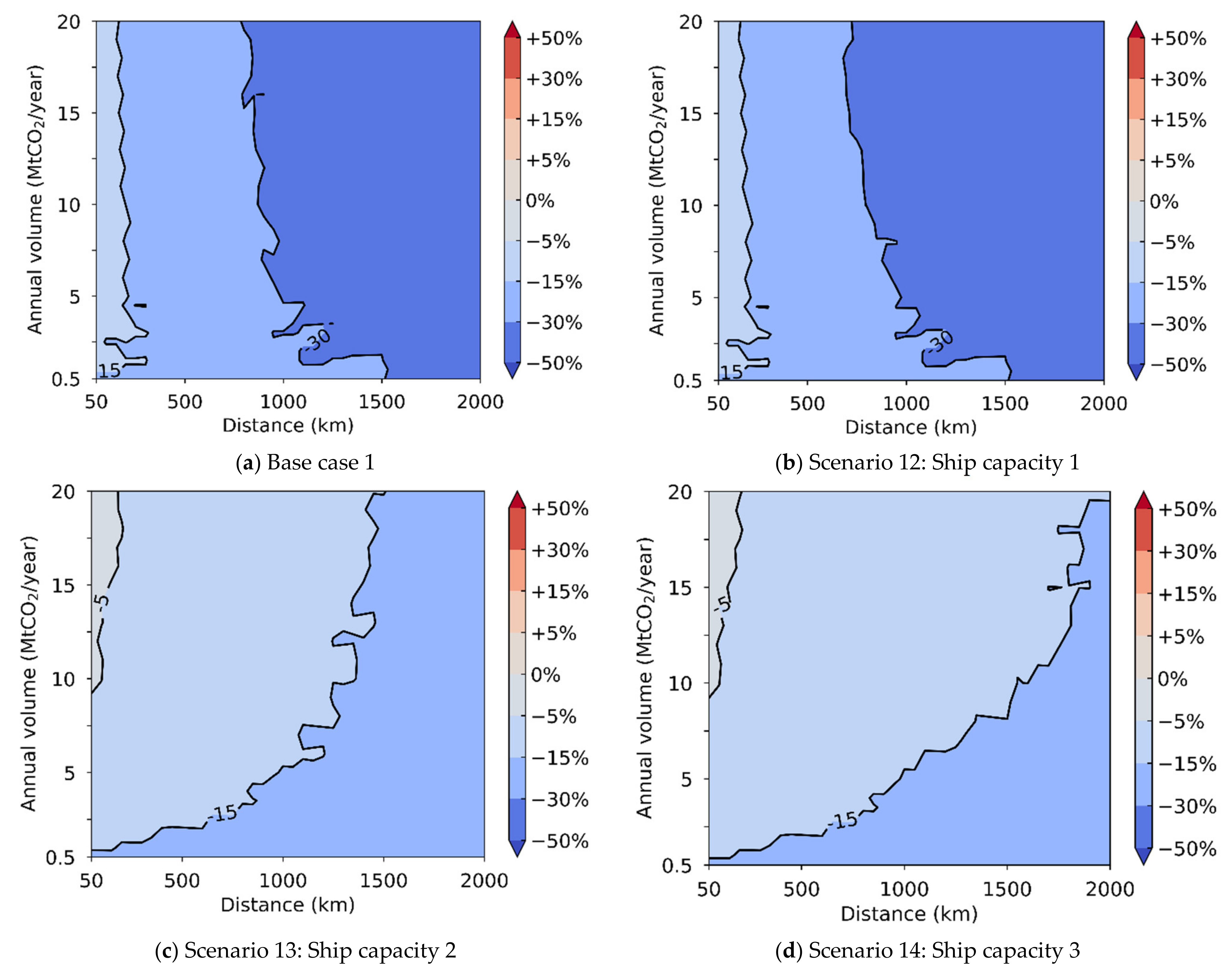
  • Both industrial feedback and recent research studies [40] have indicated that a ship capacity beyond 10 ktCO2/ship is not very likely to be feasible for the 15 barg option since the pressure limits the practical diameter that can be considered for the CO2 tank with current tank configurations. In addition, reliable cost data for 7 barg shipping are only available for capacities up to 50 ktCO2/ship. While these two limits are considered as the baseline, three scenarios (12 to 14) investigate the impact of maximum feasible ship capacity on optimal transport conditions. In the first of these scenarios (scenario 12), the maximum ship capacity for the 7 barg option is extended to 100 ktCO2, as such capacity could still be considered for transport of large volumes over long distances. Finally, scenarios 13 and 14 assume that the 15 barg option could still be feasible for ship capacity beyond 10 ktCO2/per ship. In these two scenarios, the 15 barg option is assumed to follow the same ship capacity constraint as for the 7 barg option.
A list of these scenarios and their associated characteristics are presented in Table 2.

3. Modelling

As both investments and operating costs contribute significantly to the cost of CO2 conditioned and transported, an integrated techno-economic is required to optimise and assess the characteristics and performances of the CO2 liquefaction and shipping supply chain [33,34].

3.1. Technical Modelling

3.1.1. CO2 Liquefaction

The modelling of the CO2 liquefaction process used in this study is based on our previous paper [47], which focused on understanding the optimal design and cost of this part of the CCS chain for various scenarios. While more details of the modelling approach can be found in the aforementioned paper, a brief summary of the liquefaction modelling is presented below. In addition, the resulting characteristics and costs of the liquefaction process are summarised in Table 3 for the considered impurity and purity constraint scenarios.
Modelling of the CO2 liquefaction process is the basis for an integrated techno-economic optimisation approach minimising the costs of the CO2 liquefaction process (€/tCO2). In essence, the model is used to optimise the set of process design variables presented in Figure 2 for a pre-defined set of inlet and target outlet conditions, such as temperature, pressure, and purity. Based on the results from Alabdulkarem et al. [26], the layout of the liquefaction process employed in this work is illustrated in Figure 2, and the process itself can be organised into four groups: (1) The compression train, (2) the pre-cooler, liquefier, and flash tank, (3) recirculation flash and re-compressor, and (4) the ammonia-based refrigeration cycle.
Following the capture unit, the CO2 enters the compression train ① and undergoes several stages of compression to reach a suitable liquefaction pressure. The number of compression stages is dependent on the required liquefaction pressure. Three to four stages are typical if the CO2 is available at 1 bara, but compression might also not be necessary if the CO2 is already available at high pressure, as in scenarios 3 and 4. A compression stage includes a compressor, an intercooler, and a flash separator removing condensed water.After the compression train, the CO2 stream passes into an impurity removal unit ② where potential impurities are removed if required. It is cooled and condensed through a pre-cooler ③ and a liquefier cooled by an ammonia refrigeration loop ④. It is worth noting that if the stream is pure CO2 or if all the impurities are condensed at a sufficient high liquefaction pressure, the stream is fully condensed and slightly sub-cooled after passing through the liquefier. In scenarios that consider the presence of impurities in the inlet gas, the CO2 stream may be partially condensed in the liquefier. In such situations, the uncondensed gas of the impurities together with some CO2 is purged through a flash tank ⑤, to prevent the accumulation of impurities in the process. In all situations, the condensed liquid, with or without impurities, goes through a valve ⑥ to reach the targeted delivery pressure level. The stream then enters a separator ⑦ where liquid CO2 is recovered and sent to buffer storage prior to ship transport. The gas from the separator is compressed and recirculated, to be mixed with the main stream prior to the pre-cooling stage.

3.1.2. Shipping Supply Chain

The shipping supply chain consists of four elements: (1) Buffer storage and loading, (2) shipping, (3) unloading and buffer storage, and 4) reconditioning. The modelling of the shipping supply chain is based on the CO2 shipping modules of the ICCS tool developed by SINTEF Energy Research [33,34,48]. These modules have been modified to include the best publicly available knowledge on characteristics and costs of the 7 and 15 barg shipping chains [25].
Buffer storages are required prior to and post shipping in order to integrate the differing temporalities of liquefaction and reconditioning, which are continuous processes, with shipping logistics, which is a batch process. A wide range of buffer storage capacities has been considered in the literature, but recent studies have shown that a capacity at a given harbour equal to 1.2 times the ship size under consideration is typically sufficient to ensure normal operation throughout the year, even taking weather uncertainties and maintenance periods into account [32,35]. The present study has thus adopted a buffer storage capacity of 1.2 times the ship size at each harbour. In addition to these buffer storages, logistics also require loading and unloading infrastructures, such as pumps, pipe systems, and connecting arms to transfer the CO2 to and from the ships.
Shipping logistics are the central element of the shipping supply chain. To approach continuous operation, both the individual ship capacity and the number of ships in the fleet must be optimised in order to ensure that the required transport capacity is achieved while at the same time minimising transport costs. The optimisation takes the following factors into account:
  • The duration of mooring, loading, and departure at the export hub is set to 12 h [18].
  • The average shipping speed during transport is assumed to be 26 km/h (14 knots) [18].
  • The duration of mooring, unloading, and departure at the receiving facility is considered to be 12 h in the case of an onshore harbour (base case 1), and 36 h in the case of a floating facility at sea (base case 2) [18].
  • A ship is considered to operate 8400 h per year, leaving 360 h for annual maintenance and repairs.
  • The ship capacity, and its associated characteristics, can be selected among the ones presented in Table 4 for both 7 and 15 barg shipping. As discussed in Section 2, with the exception of scenarios 12 to 14, the maximum ship capacities considered for 7 and 15 barg shipping are 50 and 10 ktCO2/ship, respectively.
  • Boil-off during ship transport is neglected [25].
After shipping, a receiving facility is required to host the buffer storage and reconditioning unit. While an onshore terminal acts as a receiving facility in the case of shipping between harbours (base case 1), a ship is used as a receiving facility in the case of shipping to an offshore site (base case 2). At the receiving facility, the CO2 must be reconditioned in order to meet the requirements for further transport and injection. This consists of pumping to reach the desired pressure, followed by heating to maintain a temperature above 5 °C. In theory, the sub-zero temperature of the CO2 after pumping could be valorised by combining this heating of the CO2 with local cooling needs (industries, LNG liquefaction, etc.) [17,49,50]. However, it is often challenging in practice to find industries with needs for such cooling near the CO2 receiving terminals. Therefore, it is assumed here that the heating of the CO2 stream after pumping is achieved using seawater through a titanium heat exchanger in order to prevent corrosion. In the case of an onshore receiving terminal, the pressure after reconditioning is set at 200 bara, which corresponds to the inlet conditions of an onshore pipeline [18]. In the case of an offshore receiving facility, this pressure is set at 90 bara, which corresponds to the inlet conditions of the riser used to transport the CO2 to the seabed [18].

3.2. Cost Assessment Methodology

All of the costs considered in this study are reported in 2017 for a north-western European location. When necessary, costs are converted into Euros using annual average exchange rates [51] and/or updated to the correct cost year using the Webci index and inflation for investment and operating costs, respectively [52,53].
The cost methodology adopted can be divided into two parts: (1) The costs of CO2 liquefaction and reconditioning processes, and (2) the costs of buffer storages, loading and unloading facilities, and ships.

3.2.1. CO2 Liquefaction and Reconditioning Processes

The CO2 liquefaction costs considered in this study are based on our previous study published in Deng et al. [47], in which the cost of liquefying 1 MtCO2/year was estimated using a bottom-up approach for both pure CO2 and the previously described impurity and purity constraint scenarios (5 to 9). These costs, summarised in Table 3, are scaled for the range of capacity considered in this study. It is worth noting that the cost of the 7 barg liquefaction is higher than the 15 barg liquefaction due to higher CAPEX and energy consumption associated with the ammonia refrigeration cycle [47]. Variable operating costs are scaled linearly with the quantity of CO2 transported, while investment costs are scaled using the cost power law presented in Equation (1) below. Annual fixed operating costs are considered to be equal to 6% of the investment costs [47]. It is worth noting that an electricity cost of 80 €/MWh is assumed [54].
The cost of the reconditioning process has been assessed using the same bottom-up approach as in Deng et al. [47].
C = C 0   ·   S S 0 n
where:
  • C is the CAPEX of the considered capacity (in M€);
  • S is the capacity under consideration (in MtCO2/year);
  • C 0 is the CAPEX for the reference capacity;
  • S 0 is the reference capacity;
n is the scaling exponent, considered to be equal to 0.85 [55] for key costs linked to the rotating equipment.

3.2.2. Buffer Storage, Loading and Unloading Facilities, and Ships

For these units, investment costs are scaled directly from the reference capacity. Investment costs associated with the buffer storage are assumed to be 550 and 920 €/m3 for the 7 and 15 barg shipping options, respectively [40], while their annual fixed operating costs represent 6% of investment costs [56].
The investment costs of loading and unloading facilities are scaled linearly from a reference case, assuming 7.9 M€ for a 3 MtCO2/year of capacity for each facility. The annual operating cost of these facilities is assumed to represent 2% of investment costs [57].
For ships, investment and fixed operating costs are presented in Table 4. Investment costs of a ship are a function of the ship capacity and are based on the regressions established by Element Energy Limited [40] for 7 and 15 barg shipping. It is worth noting that as in the case of buffer storage, the cost of a 15 barg shipping is about twice that for a 7 barg shipping of the same capacity.
In order to understand the impact of maximum ship capacity in scenarios 12 to 14, it is here assumed that the regressions of Element Energy Limited [40] can be extrapolated beyond their domains of proven validity (50 and 10 ktCO2/ship, respectively, for 7 and 15 barg shipping). The validity of this assumption is discussed in Section 5.4 in the context of the results of scenarios 12 to 14. The annual operating cost of a ship is set at 5% of the ship CAPEX [40], while variable operating costs are calculated based on a fuel cost of 325 €/tfuel [58] and harbour fees of 1.1 €/tCO2 at each harbour [17]. Finally, for ships used as receiving terminals in the case of CO2 transport to an offshore site, their costs are assumed to be 20% higher than those for a standard ship. This increase accounts for construction and installation requirements protecting against harsher weather conditions, the need to generate electricity to drive reconditioning, as well as local infrastructure at the offshore site [34].

3.3. Cost Performance Metric

The cost of CO2 conditioning and transport [20], expressed by Equation (2), is used in this study as a cost performance metric for both optimisation and comparison of the transport chains. This cost performance metric is computed considering a real discount rate of 8%, a project duration of 25 years, and an operating rate of 85%.
Finally, investments are expected to be spread over a 3-year period with a cost allocation of 40%, 30%, and 30%.
CO 2   conditioning   and   transport   cost = Annualised   investment + Annual   OPEX Annual   amount   of   CO 2   transported

4. Results

In this section, 7 and 15 barg shipping are compared for the transport of pure CO2 between harbours (base case 1), and transport to an offshore site (base case 2).
Since the comparison of 7 and 15 barg shipping is performed for a combination of wide ranges of transport distances and annual volumes for both the base cases and the scenarios considered in this study, the results are presented as a series of cost comparison maps. As can be seen in Figure 3, the transport distance and annual volume are displayed as the x- and y-axes, respectively, while the relative costs of 7 barg compared to 15 barg shipping are represented using colour coding. The darker the blue colour is for the combination of distance and volume, the cheaper it is to ship CO2 at 7 barg compared to 15 barg shipping. On the other hand, the darker the red colour is, the more expensive it is to ship CO2 at 7 barg compared to 15 barg shipping.
As discussed earlier, both CO2 liquefaction and the shipping chain have been optimised to minimise the transport cost for each combination of transport distance and annual volume. Since the number of ships and their capacities are not continuous functions, this mixed-integer problem results in coarse transitions between the cost reduction areas, and in some cases even the creation of bubbles.
Previous studies [33,34] have shown that, depending on transport distances and annual volumes, the transport of CO2 by pipeline could be more cost-efficient than using shipping. Therefore, it is important to be aware of when pipeline transport outperforms ship transport, at both 7 and 15 barg, to identify the optimal conditions for ship-based transport. This is displayed on the base case cost maps using a stippled, cyan-coloured line, which indicates the frontier between where the pipeline- and shipping-based transport of CO2 are cost-optimal. To the left of this line, pipelines offer the most cost-efficient transport solution, while shipping is the most cost-efficient solution to the right of the line. Details of the techno-economic modelling of the pipeline-based transport of CO2 are presented in Appendix A.
The cost comparison maps offer an efficient way of comparing the costs associated with the 7 and 15 barg options for a wide range of transport distances and annual volumes. However, they do not provide insights into actual CO2 conditioning and transport costs or the breakdown of these. Since these parameters also constitute valuable outcomes from our study, we provide more details on these in Appendix B and Appendix C.

4.1. CO2 Shipping between Harbours

The costs of transporting pure CO2 between two harbours (base case 1) at 7 barg compared to 15 barg shipping are shown in Figure 3a,b. The figures show that shipping at 7 barg is the most cost-efficient solution for all combinations of transport distance and annual volume under consideration. Furthermore, shipping at 7 barg enables significant cost reductions for the vast majority of relevant transport distances and annual volumes. Most cases result in cost reductions beyond 15%, and reductions greater than 30% may be achieved for distances of about 1000 km and larger. This is even more striking when looking only at the area where shipping is more cost-efficient than pipeline-based transport (i.e., to the right of the cyan line on the maps). Here, 7 barg shipping enables cost reduction beyond 30% compared to 15 barg shipping for more than two-thirds of the combinations. These results show that even in the near term, for which small-scale deployment is most relevant, 7 barg shipping is the most cost-efficient option and could enable cost reduction beyond 15%. Such reductions are also significant in terms of absolute CO2 conditioning and transport costs, as for distances greater than 350 and 1000 km, the 7 barg shipping option results in costs of at least 5 and 10 €/tCO2, respectively, lower than for the 15 barg option (Figure 3b).
In order to explain these cost reductions, it is important to understand the logistic aspects of both shipping options. Optimal ship capacity (tCO2/ship) and fleet sizes are shown in Figure 4a,b. Here, the colour coding indicates ship capacity, while the pink lines represent the number of ships in the fleet. Whereas small ship capacities appear to be cost-optimal for shorter distances and/or lower volumes, large ships tend rapidly to become more cost-efficient as distances and volumes increase, all the way up to the maximum permitted ship sizes. While this observation is valid for both 7 and 15 barg shipping options, it results in smaller ship capacities for 15 barg-based shipping since its maximum ship capacity is smaller (10 ktCO2/ship versus 50 ktCO2/ship), requiring more ships to be deployed than for 7 barg-based shipping carrying the same volumes.
Considering this, the lower costs achieved by the 7 barg-based transport chains, despite a higher liquefaction cost, can be explained by two main reasons that enable significantly lower ship CAPEX than for the 15 barg shipping as can be observed in the cost breakdowns presented in Appendix C. Firstly, for the same ship capacity, investment in a 7 barg shipping is about half of that for a 15 barg shipping. Secondly, larger ship capacities and smaller fleets can be used for 7 barg shipping, which enables further costs savings based on the economy of scale in ship CAPEX that can be observed in Table 4.

4.2. CO2 Shipping to an Offshore Site

The costs of transporting pure CO2 to an offshore site (base case 2) at 7 barg compared to 15 barg shipping are shown in the cost comparison maps in Figure 5a,b. As for the previous case involving shipping between harbours, 7 barg shipping is shown to be the most cost-efficient option in all cases. In fact, an even greater potential for cost reductions is observed here. The 7 barg shipping enables major reductions (beyond 30%) compared to 15 barg in most cases. Furthermore, most of the combinations of transport distance and annual volume for which cost reductions are less than 30% correspond to those for which an offshore pipeline would the preferred option (combinations lying to the left of the cyan line). As was the case for shipping between harbours, these cost reductions are also significant in absolute terms for CO2 conditioning and transport costs. The 7 barg shipping enables cost reductions beyond 10 €/tCO2 for transport distances greater than 650 km, and even exceeds a reduction of 15 €/tCO2 for distances greater than 1200 km.
The direct transport of CO2 by ship is currently not the preferred option when it comes to accessing offshore CO2 storage sites due to uncertainties, high levels of investment, and limited opportunities for economies of scale in the case of stepwise capacity deployment [24]. However, these results show that 7 barg shipping may be the key to unlocking cost-efficient deployment of such a solution.

5. Discussions

The impact of the different parameters on the comparison of 7 and 15 barg conditions for CO2 shipping is here explored for the case of transport of CO2 between harbours, unless otherwise indicated, for the scenarios presented in Section 2. For each of these scenarios, it is worth noting that the liquefaction process and the shipping supply are re-optimised according to the characteristics of the scenario considered.

5.1. Impact of CO2 Pressure Prior to the Liquefaction Process

It has been assumed in the base cases that the CO2 liquefaction process receives CO2 from the capture facility at 1 bara and near ambient temperature. While this assumption is representative of a CO2 liquefaction process located close to the CO2 capture facility, an alternative and relevant scenario is that the CO2 stream sent to CO2 liquefaction is already pressurised. This situation may be representative for cases in which the CO2 comes from inland emitters or an industrial cluster. Indeed, in such cases, it is likely that the CO2 would be transported at high pressure via a pipeline prior to liquefaction and ship transport. In such cases, the CO2 would typically be expected to be available at 90 bara [18] prior to its liquefaction and shipping. This corresponds to the outlet pressure of an onshore pipeline prior to liquefaction. Two scenarios (3 and 4) thus seek to understand if, and in what ways, optimal transport conditions are impacted if the CO2 to be transported is available at 90 bara prior to its liquefaction. Note that, while inlet pressure may impact the selection of the type of refrigeration cycle (internal cooling versus external cooling), the ammonia-based liquefaction presented in Section 3.1.1 is also considered in the evaluations of scenarios 3 and 4.
The results of these scenarios are presented in Figure 6 and Figure 7 for cases involving transport between harbours and transport to an offshore site, respectively. The results show that in both cases, 7 barg shipping appears to enable much greater relative cost reductions compared to the corresponding base case. For example, in the case of transport between harbours, 7 barg shipping can result in cost reductions beyond 30% compared with 15 barg shipping in almost all the cases where shipping is the cost-optimal means of transport. Similarly, in the case of shipping to an offshore site, the 7 barg option enables cost reductions greater than 30% in all relevant cases and beyond 50% in many cases.
However, when looking at absolute cost reductions in CO2 avoidance cost, scenarios 3 and 4 provide outcomes that are in fact very similar to their corresponding base cases. The reason why this difference appears stronger in relative terms in scenario 3 and 4 is that the compression of CO2 from 1 to 90 bara is now not included within the system boundaries. As a result, CO2 conditioning and transport costs are lower in scenarios 3 and 4 than in the base cases. Since the absolute cost reduction [€/tCO2] is compared to smaller CO2 conditioning and transport costs, it appears stronger in relative terms than in the base cases.

5.2. Impact of Impurities and Purity Constraints

Since both the presence of impurities in the CO2 stream after capture and possible purity constraints have been shown to have an impact on CO2 transport design and costs [20,21,43], it is important to evaluate whether this also has an effect on the comparison of the 7 and 15 barg shipping options. In the case of transport by ship, impurities can impact both the CO2 conditioning and transport of a given option through the energy requirements and the design of the liquefaction process, the density of the resulting liquid CO2, the energy requirement and design of the reconditioning process, and possibly material selection if impurities are corrosive.
These effects are here investigated through three impurity scenarios (5 to 7) with different types and levels of impurities, as described in Section 2, as well as two scenarios (8 and 9) considering additional purity requirements (≥99% and ≥99.9%, respectively) for the post-combustion membrane impurity case. Corrosion is not regarded as an issue in the cases considered here. The results of the two sets of scenarios are presented in Figure 8b–f, while the pure CO2 base case is repeated from Figure 3a to Figure 8a for ease of comparison.
The results show that cases with impurities lead to similar conclusions as for the base case. The 7 barg option continues to remain the most cost-efficient shipping solution for all the cases considered. Compared to the case of pure CO2, scenarios involving impurities appear to give us a slightly lower relative cost reduction potential of 7 barg compared to the 15 barg shipping option. This is observed through a minor shift of iso-cost reduction curves towards the right of the figures. In the purity requirement scenarios, the 99% purity constraint (Figure 8e) appears not to deviate significantly from the base case since the purity requirement is inherently met by the liquefaction process for both the 7 and 15 barg transport options. In the case of the 99.9% purity constraint scenario (Figure 8f), the cost reduction potential of the 7 barg option remains significant, although a slight decrease is observed.
While minor decreases in relative cost reduction potential are observed for these scenarios, it is important to be aware that the normalised cost reduction potentials [€/CO2] enabled by the 7 barg option are almost identical for both the base case and all the impurity and purity constraint scenarios. Any variation in relative cost reduction potential is linked mainly to an increase in the cost of liquefaction and transport for both the 7 and 15 barg options in these scenarios, rather than a change in normalised cost reduction potential. In any event, the shipping at 7 barg remains the most cost-efficient options in all the impurity and purity constraint scenarios considered in this study.

5.3. Impact of Uncertainties in Ship Investment Costs

It is important to consider modelling uncertainties in order to produce a sound techno-economic analysis [59]. The impact of inherent uncertainties in 7 and 15 barg shipping investment costs on the comparison of the two shipping pressures were investigated through scenarios 10 and 11 and are illustrated in Figure 9. Since the results from the base case show a very strong advantage for the 7 barg shipping option, the scenarios are testing pessimistic uncertainty assumptions for the 7 barg option with regards to the ship CAPEX regression established by Element Energy Limited [40]. These pessimistic scenarios also seek to potentially higher costs that may be associated with additional safety measures for the 7 barg shipping chain to control the margin from the triple point. Indeed, scenarios 10 and 11 assume that these regressions have both underestimated the 7 barg shipping CAPEX and overestimated the 15 barg shipping CAPEX. While the base case is shown in Figure 9a, the results of the two scenarios, when the ship CAPEX regressions are assumed to be overestimated/underestimated by respectively 10 and 20% compared to the base case, are presented in Figure 9b,c.
The results show that, despite the pessimistic assumptions in scenarios 10 and 11, the 7 barg transport option remains the most cost-efficient solution for all combinations of transport distance and annual volume. However, the cost reduction potential of the 7 barg option relative to the 15 barg case is reduced compared to the base case. This reduction is particularly marked in scenario 11, where only some of the cases with both capacities beyond 6 MtCO2/year and transport distances greater than 1700 km are able to achieve cost reduction beyond 30%. However, it is important to note that even with such pessimistic scenarios for the 7 barg shipping option, it still enables cost reductions greater than 15% for most of the capacity and distance combinations for which ship-based transport would be preferred to pipeline transport.

5.4. Impact of Maximum Ship Capacity

An important difference that emerged in the characteristics between the 7 and 15 barg shipping chains was the maximum ship capacity that could realistically be considered. Recent studies [40] and feedback from the industry both indicate that ship capacities greater than 10 ktCO2/ship are most likely unfeasible for the 15 barg option with conventional tank configurations, whereas capacities of at least up to 50 ktCO2/year are foreseen for the 7 barg option. In order to understand the impact of these limitations on the transport option comparison, three scenarios are investigated: (1) Scenario 12, in which the maximum ship capacity for the 7 barg option is increased to 100 ktCO2 as such capacities could be relevant for the transport of large volumes of CO2 over long distances, (2) scenario 13, in which it is assumed that 15 barg shipping could be built for capacities of up to 50 ktCO2, and (3) scenario 14, in which it is assumed that both 7 and 15 barg shipping could be built for capacities up to 100 ktCO2. In all these scenarios, it is assumed that the ship CAPEX still follows the regressions established by Element Energy Limited, even if the ship capacity lies outside the regression range. The results of the evaluation of these three scenarios are presented in Figure 10b–d, together with the base case for comparison (Figure 10a).
The results from scenario 12 show that a greater maximum ship capacity solely for the 7 barg option has little impact on its cost reduction potential, although a minor improvement is observed for combinations involving large annual volumes and long transport distances. Even when considering identical maximum ship capacities for the 7 and 15 barg options, as in scenarios 13 and 14, the 7 barg option remains the most attractive solution in terms of costs, although the cost reduction potential is significantly reduced compared to the base case. For most combinations, the cost reduction potential lies between 5 and 15%. While it is not possible to achieve cost reductions greater than 30% anymore, cost reductions beyond 15% can still be enabled by the 7 barg option. Such reductions are possible primarily for combinations involving small to medium capacities over medium to long transport distances, and for long distances.
While the feasibility of large-capacity 15 barg shipping may in theory reduce the cost reduction potential of the 7 barg shipping option, both the study published by Element Energy Limited and feedback from the industry indicate that ship capacities greater than 10 ktCO2/ship would very likely be infeasible for the 15 barg option with current tank configurations, since the pressure limits the practical CO2 tank diameters. One possibility would be to consider new tank architectures involving small-diameter vertical tanks. However, ships equipped with such tank configurations are foreseen to be more expensive than those modelled for the 15 barg CAPEX regressions published by Element Energy Limited.

6. Conclusions

The pipeline has historically been the preferred means to transport CO2 due to its low cost for short distances and opportunities for economies of scale. However, as low cost for small scale deployment and low investments make CO2 shipping a low risk and flexible option for upcoming CCS projects, the question of optimal transport pressure remained. In the present study, we carried out an in-depth comparison of the 7 and 15 barg transport pressure options for a wide range of annual volumes and transport distances, including sensitivity analyses on four key parameters/uncertainties. The results clearly show that the shipping of CO2 at 7 barg is more cost-efficient than at 15 barg and could enable significant cost reductions (beyond 15% in nearly all cases and beyond 30% in most cases).
Despite the significant cost reduction potential of 7 barg, it is however likely that shipping of CO2 at 15 barg will still be selected for very near term implementations, as in the Longship project [42], due to its technological maturity. To realise this cost reduction potential, further efforts are still needed to demonstrate at large-scale that shipping of CO2 can be safely and reliably operated at 7 barg. For example, it is key to prevent the formation of solid CO2 (both dry ice and hydrates) in the conditioning and transport supply chain to prevent blockage and abnormal operations. Furthermore, opportunities to reduce costs through technological improvements, such as cold energy recovery during offloading operations, shall be further investigated. Finally, while 7 barg shipping can be expected to be the preferred solution for new development, once it has been demonstrated to be reliable and safe at large-scale, a question worth exploring in future work is if retrofitting an existing 15 barg shipping chain to 7 barg could be a financially attractive solution [36].

Author Contributions

Conceptualization, S.R., H.D. and G.S.; formal analysis, S.R., H.D. and G.S.; methodology, S.R., H.D. and G.S.; writing—original draft, S.R.; writing—review and editing, S.R., H.D., G.S. and T.G. All authors have read and agreed to the published version of the manuscript.

Funding

This publication has been produced with support from the NCCS Research Centre, performed under the Norwegian research program Centres for Environment-friendly Energy Research (FME). The authors acknowledge the following partners for their contributions: Aker Carbon Capture, Ansaldo Energia, Baker Hughes, CoorsTek Membrane Sciences, Equinor, Fortum Oslo Varme, Gassco, KROHNE, Larvik Shipping, Lundin Norway, Norcem, Norwegian Oil and Gas, Quad Geometrics, Stratum Reservoir, Total, Vår Energi, Wintershall DEA, and the Research Council of Norway (257579).

Acknowledgments

The authors would like to thank Thomas de Cazenove, Clement Merat, and Petter Nekså for their useful comments and suggestions.

Conflicts of Interest

The authors declare no conflict of interest.

Abbreviations

CAPEXCapital expenditures
CCSCarbon capture and storage
IGCCIntegrated gasification combined cycle
OPEXOperating expenditures

Appendix A. Modelling of Pipeline-Based CO2 Transport

Pipeline-based transport has been modelled in this study using the iCCS tool developed by SINTEF Energy Research, which has already been presented in detail in the literature [33,34,48]. Pipeline-based transport comprises two parts: The conditioning and the pipeline export.
The conditioning process consists primarily of an intercooled multi-stage compression train in order to achieve the desired pressure at the inlet of the pipeline (150 bara for an onshore pipeline, and 200 bara for an offshore pipeline).
The pipeline export stage primarily involves the pipeline itself and its reboosting stations. As part of the pipeline export design procedure (Figure A1), the external pipeline diameter is optimised in order to minimise transport costs while maintaining pressure above supercritical conditions at all points along the pipeline. In the case of an onshore pipeline, a reboosting station is included at the end of the pipeline in order to deliver the CO2 at 200 bar, which corresponds to the inlet pressure of an offshore pipeline. On the other hand, in the case of offshore pipelines, offshore reboosting stations are not considered due to their prohibitive costs. In order to include the most recent knowledge available, we have selected the pipeline cost model developed by Knoope et al. [60], and not the CO2 Europipe [61] model used in some of our previous studies [33,34].

Appendix B. CO2 Conditioning and Transport Costs

In order to provide a greater insight into CO2 conditioning and transport costs for the means of transport considered in this study (7 and 15 barg shipping, and pipelines), the following sections provide cost estimates for the transport of pure CO2 as a function of annual volume and transport distances. Appendix B.1 presents estimates for transport between harbours and onshore locations, while Appendix B.2 provides estimates in the case of transport to an offshore site.
Please note that the value ranges on the y-axes are not the same in all figures.
Figure A1. Pipeline design procedure.
Energies 14 05635 g0a1

Appendix B.1. CO2 Conditioning and Transport Costs for Transport between Two Harbours/Onshore Locations

Figure A2. CO2 conditioning and transport costs as a function of transport distance and annual volume when transporting pure CO2 between two harbours by ship at 15 barg.
Energies 14 05635 g0a2
Figure A3. CO2 conditioning and transport costs as a function of transport distance and annual volume when transporting pure CO2 between two harbours by ship at 7 barg.
Energies 14 05635 g0a3
Figure A4. CO2 conditioning and transport costs as a function of transport distance and annual volume when transporting pure CO2 between two onshore locations using an onshore pipeline.
Energies 14 05635 g0a4

Appendix B.2. CO2 Conditioning and Transport Costs for Transport to an Offshore Site

Figure A5. CO2 conditioning and transport costs as a function of transport distance and annual volume when transporting pure CO2 to an offshore site by ship at 15 barg.
Energies 14 05635 g0a5
Figure A6. CO2 conditioning and transport costs as a function of transport distance and annual volume when transporting pure CO2 to an offshore site by ship at 7 barg.
Energies 14 05635 g0a6
Figure A7. CO2 conditioning and transport costs as a function of transport distance and annual volume when transporting pure CO2 to an offshore site using an offshore pipeline.
Energies 14 05635 g0a7

Appendix C. Cost Breakdowns

In order to provide greater insight into the underlying contributing elements to the CO2 conditioning and transport costs, cost breakdowns are presented for the means of transport considered in this study (7 and 15 barg shipping, and pipelines) as a function of annual volume and transport distance. Appendix C.1 presents estimates for transport between harbours or onshore locations, while Appendix C.2 provides estimates in cases of transport to an offshore site.
Please note that the value ranges on the y-axes are not the same in all figures.

Appendix C.1. CO2 Conditioning and Transport Cost Breakdowns for Transport between Two Harbours/Onshore Locations

Figure A8. Cost breakdown of CO2 conditioning and transport costs as a function of transport distance (d in km) and annual volume (V in MtCO2/year) when transporting pure CO2 between two harbours by ship at 15 barg.
Energies 14 05635 g0a8
Figure A9. Cost breakdown of CO2 conditioning and transport costs as a function of transport distance (d in km) and annual volume (V in MtCO2/year) when transporting pure CO2 between two harbours by ship at 7 barg.
Energies 14 05635 g0a9
Figure A10. Cost breakdown of CO2 conditioning and transport costs as a function of transport distance (d in km) and annual volume (V in MtCO2/year) when transporting pure CO2 between two onshore locations using an onshore pipeline (the upper y-axis is here limited to 80 €/tCO2, which means that some of the cost breakdown data are not displayed in full).
Energies 14 05635 g0a10

Appendix C.2. CO2 Conditioning and Transport Cost Breakdowns for Transport to an Offshore Site

Figure A11. Cost breakdown of CO2 conditioning and transport costs as a function of transport distance (d in km) and annual volume (V in MtCO2/year) when transporting pure CO2 to an offshore site by ship at 15 barg.
Energies 14 05635 g0a11
Figure A12. Cost breakdown of CO2 conditioning and transport costs as a function of transport distance (d in km) and annual volume (V in MtCO2/year) when transporting pure CO2 to an offshore site by ship at 7 barg.
Energies 14 05635 g0a12
Figure A13. Cost breakdown of CO2 conditioning and transport costs as a function of transport distance (d in km) and annual volume (V in MtCO2/year) when transporting pure CO2 to an offshore site using an offshore pipeline (the upper y-axis is here limited to 80 €/tCO2, which means that some of the cost breakdown data are not displayed in full).
Energies 14 05635 g0a13

References

  1. Energy Technology Perspective; IEA: Paris, France, 2020.
  2. Mølnvik, M.J.; Aarlien, R.; Henriksen, P.P.; Munkejord, S.T.; Tangen, G.; Jakobsen, J.P. BIGCCS Innovations—Measures to Accelerate CCS Deployment. Energy Procedia 2016, 86, 79–89. [Google Scholar] [CrossRef] [Green Version]
  3. Gardarsdottir, S.; De Lena, E.; Romano, M.; Roussanaly, S.; Voldsund, M.; Pérez-Calvo, J.-F.; Berstad, D.; Fu, C.; Anantharaman, R.; Sutter, D.; et al. Comparison of technologies for CO2 capture from cement production—Part 2: Cost analysis. Energies 2019, 12, 542. [Google Scholar] [CrossRef] [Green Version]
  4. Abanades, J.C.; Arias, B.; Lyngfelt, A.; Mattisson, T.; Wiley, D.E.; Li, H.; Ho, M.T.; Mangano, E.; Brandani, S. Emerging CO2 capture systems. Int. J. Greenh. Gas Control 2015, 40, 126–166. [Google Scholar] [CrossRef] [Green Version]
  5. Roussanaly, S.; Berghout, N.; Fout, T.; Garcia, M.; Gardarsdottir, S.; Nazir, S.M.; Ramirez, A.; Rubin, E.S. Towards improved cost evaluation of Carbon Capture and Storage from industry. Int. J. Greenh. Gas Control 2021, 106, 103263. [Google Scholar] [CrossRef]
  6. Assessment of Emerging CO2 Capture Technologies and their Potential to Reduce Costs; 2014/TR4; IEAGHG: Cheltenham, UK, 2014.
  7. Further Assessments of Emerging CO2 Capture Technologies for the Power Sector and their Potential to Reduce Costs; IEAGHG: Cheltenham, UK, 2019.
  8. Cleanker Project. Clean Clinker by Calcium Looping for Low-CO2 Cement. Available online: http://www.cleanker.eu/the-project/objectives.html (accessed on 1 May 2021).
  9. Global status of CCS; Global CCS Institute: Docklands, Australia, 2019.
  10. CO2RE Facilities Database; Global CCS Institute: Docklands, Australia, 15 September 2020.
  11. Morbee, J.; Serpa, J.; Tzimas, E. Optimised deployment of a European CO2 transport network. Int. J. Greenh. Gas Control 2012, 7, 48–61. [Google Scholar] [CrossRef]
  12. d’Amore, F.; Romano, M.; Bezzo, F. Optimal design of European supply chains for carbon capture and storage from industrial emission sources including pipeline and ship transport. Int. J. Greenh. Gas Control 2021, 109, 103372. [Google Scholar] [CrossRef]
  13. Munkejord, S.T.; Hammer, M.; Løvseth, S.W. CO2 transport: Data and models—A review. Appl. Energy 2016, 169, 499–523. [Google Scholar] [CrossRef]
  14. Koornneef, J.; Spruijt, M.; Molag, M.; Ramírez, A.; Turkenburg, W.; Faaij, A. Quantitative risk assessment of CO2 transport by pipelines—A review of uncertainties and their impacts. J. Hazard. Mater. 2010, 177, 12–27. [Google Scholar] [CrossRef] [PubMed]
  15. Knoope, M.M.J.; Raben, I.M.E.; Ramírez, A.; Spruijt, M.P.N.; Faaij, A.P.C. The influence of risk mitigation measures on the risks, costs and routing of CO2 pipelines. Int. J. Greenh. Gas Control 2014, 29, 104–124. [Google Scholar] [CrossRef]
  16. McCoy, S.T.; Rubin, E.S. An engineering-economic model of pipeline transport of CO2 with application to carbon capture and storage. Int. J. Greenh. Gas Control 2008, 2, 219–229. [Google Scholar] [CrossRef]
  17. Roussanaly, S.; Bureau-Cauchois, G.; Husebye, J. Costs benchmark of CO2 transport technologies for a group of various size industries. Int. J. Greenh. Gas Control 2013, 12, 341–350. [Google Scholar] [CrossRef] [Green Version]
  18. The Costs of CO2 Transport, Post-Demonstration CCS in the EU; Zero Emission Platform: Brussels, Belgium, 2011.
  19. Wei, N.; Li, X.; Wang, Q.; Gao, S. Budget-type techno-economic model for onshore CO2 pipeline transportation in China. Int. J. Greenh. Gas Control 2016, 51, 176–192. [Google Scholar] [CrossRef]
  20. Skaugen, G.; Roussanaly, S.; Jakobsen, J.; Brunsvold, A. Techno-economic evaluation of the effects of impurities on conditioning and transport of CO2 by pipeline. Int. J. Greenh. Gas Control 2016, 54 Pt 2, 627–639. [Google Scholar] [CrossRef] [Green Version]
  21. Porter, R.T.J.; Mahgerefteh, H.; Brown, S.; Martynov, S.; Collard, A.; Woolley, R.M.; Fairweather, M.; Falle, S.A.E.G.; Wareing, C.J.; Nikolaidis, I.K.; et al. Techno-economic assessment of CO2 quality effect on its storage and transport: CO2QUEST: An overview of aims, objectives and main findings. Int. J. Greenh. Gas Control 2016, 54 Pt 2, 662–681. [Google Scholar] [CrossRef] [Green Version]
  22. Fimbres Weihs, G.A.; Wiley, D.E. Steady-state design of CO2 pipeline networks for minimal cost per tonne of CO2 avoided. Int. J. Greenh. Gas Control 2012, 8, 150–168. [Google Scholar] [CrossRef]
  23. Kim, C.; Kim, K.; Kim, J.; Ahmed, U.; Han, C. Practical deployment of pipelines for the CCS network in critical conditions using MINLP modelling and optimization: A case study of South Korea. Int. J. Greenh. Gas Control 2018, 73, 79–94. [Google Scholar] [CrossRef]
  24. Feasibility Study for Full-Scale CCS in Norway; Ministry of Petroleum and Energy: Oslo, Norway, 2016.
  25. Al Baroudi, H.; Awoyomi, A.; Patchigolla, K.; Jonnalagadda, K.; Anthony, E.J. A review of large-scale CO2 shipping and marine emissions management for carbon capture, utilisation and storage. Appl. Energy 2021, 287, 116510. [Google Scholar] [CrossRef]
  26. Alabdulkarem, A.; Hwang, Y.; Radermacher, R. Development of CO2 liquefaction cycles for CO2 sequestration. Appl. Therm. Eng. 2012, 33, 144–156. [Google Scholar] [CrossRef]
  27. Lee, S.G.; Choi, G.B.; Lee, C.J.; Lee, J.M. Optimal design and operating condition of boil-off CO2 re-liquefaction process, considering seawater temperature variation and compressor discharge temperature limit. Chem. Eng. Res. Des. 2017, 124, 29–45. [Google Scholar] [CrossRef]
  28. Jeon, S.H.; Kim, M.S. Effects of impurities on re-liquefaction system of liquefied CO2 transport ship for CCS. Int. J. Greenh. Gas Control 2015, 43, 225–232. [Google Scholar] [CrossRef]
  29. Decarre, S.; Berthiaud, J.; Butin, N.; Guillaume-Combecave, J.-L. CO2 maritime transportation. Int. J. Greenh. Gas Control 2010, 4, 857–864. [Google Scholar] [CrossRef] [Green Version]
  30. Vermeulen, T.N. Knowledge Sharing Report—CO2 Liquid Logistics Shipping Concept (LLSC): Overall Supply Chain Optimization; 3112001; Tebodin Netherlands, B.V.: The Hague, The Netherlands, 21 June 2011. [Google Scholar]
  31. Climate Change 2014: Synthesis Report. Contribution of Working Groups I, II and III to the Fifth Assessment Report of the Intergovernmental Panel on Climate Change; IPCC: Geneva, Switzerland, 2014. [Google Scholar]
  32. Jung, J.-Y.; Huh, C.; Kang, S.-G.; Seo, Y.; Chang, D. CO2 transport strategy and its cost estimation for the offshore CCS in Korea. Appl. Energy 2013, 111, 1054–1060. [Google Scholar] [CrossRef]
  33. Roussanaly, S.; Jakobsen, J.P.; Hognes, E.H.; Brunsvold, A.L. Benchmarking of CO2 transport technologies: Part I—Onshore pipeline and shipping between two onshore areas. Int. J. Greenh. Gas Control 2013, 19, 584–594. [Google Scholar] [CrossRef] [Green Version]
  34. Roussanaly, S.; Brunsvold, A.L.; Hognes, E.S. Benchmarking of CO2 transport technologies: Part II—Offshore pipeline and shipping to an offshore site. Int. J. Greenh. Gas Control 2014, 28, 283–299. [Google Scholar] [CrossRef] [Green Version]
  35. Bjerketvedt, V.S.; Tomasgard, A.; Roussanaly, S. Optimal design and cost of ship-based CO2 transport under uncertainties and fluctuations. Int. J. Greenh. Gas Control 2020, 103, 103190. [Google Scholar] [CrossRef]
  36. Bjerketvedt, V.; Tomasgaard, A.; Roussanaly, S. Deploying a shipping infrastruture to enable CCS from Norwegian industries. Accept. J. Clean. Prod. 2021. [Google Scholar]
  37. Kang, K.; Seo, Y.; Chang, D.; Kang, S.-G.; Huh, C. Estimation of CO2 Transport Costs in South Korea Using a Techno-Economic Model. Energies 2015, 8, 2176–2196. [Google Scholar] [CrossRef] [Green Version]
  38. Feasibility Study for Ship Based Transport of Ethane to Europe and Back Hauling of CO2 to the USA; IEAGHG: Cheltenham, UK, 2017.
  39. Seo, Y.; Huh, C.; Lee, S.; Chang, D. Comparison of CO2 liquefaction pressures for ship-based carbon capture and storage (CCS) chain. Int. J. Greenh. Gas Control 2016, 52, 1–12. [Google Scholar] [CrossRef]
  40. Shipping CO2—UK Cost Estimation Study; Element Energy Limited: Cambridge, UK, 2018.
  41. Northern Lights Contribution to Benefit Realisation; Equinor: Trondheim, Norway, 2019.
  42. Longship—Carbon Capture and Storage; Norwegian Ministry of Petroleum and Energy: Oslo, Norway, 2020.
  43. Brunsvold, A.; Jakobsen, J.P.; Mazzetti, M.J.; Skaugen, G.; Hammer, M.; Eickhoff, C.; Neele, F. Key findings and recommendations from the IMPACTS project. Int. J. Greenh. Gas Control 2016, 54 Pt 2, 588–598. [Google Scholar] [CrossRef]
  44. Voldsund, M.; Gardarsdottir, S.; De Lena, E.; Pérez-Calvo, J.-F.; Jamali, A.; Berstad, D.; Fu, C.; Romano, M.; Roussanaly, S.; Anantharaman, R.; et al. Comparison of technologies for CO2 capture from cement production—Part 1: Technical evaluation. Energies 2019, 12, 559. [Google Scholar] [CrossRef] [Green Version]
  45. Roussanaly, S.; Anantharaman, R. Cost-optimal CO2 capture ratio for membrane-based capture from different CO2 sources. Chem. Eng. J. 2017, 327, 618–628. [Google Scholar] [CrossRef] [Green Version]
  46. Roussanaly, S.; Vitvarova, M.; Anantharaman, R.; Berstad, D.; Hagen, B.; Jakobsen, J.; Novotny, V.; Skaugen, G. Techno-economic comparison of three technologies for pre-combustion CO2 capture from a lignite-fired IGCC. Front. Chem. Sci. Eng. 2020, 14, 436–452. [Google Scholar] [CrossRef]
  47. Deng, H.; Roussanaly, S.; Skaugen, G. Techno-economic analyses of CO2 liquefaction: Impact of product pressure and impurities. Int. J. Refrig. 2019, 103, 301–315. [Google Scholar] [CrossRef]
  48. Jakobsen, J.; Roussanaly, S.; Anantharaman, R. A techno-economic case study of CO2 capture, transport and storage chain from a cement plant in Norway. J. Clean. Prod. 2017, 144, 523–539. [Google Scholar] [CrossRef] [Green Version]
  49. Aspelund, A.; Gundersen, T. A liquefied energy chain for transport and utilization of natural gas for power production with CO2 capture and storage—Part 1. Appl. Energy 2009, 86, 781–792. [Google Scholar] [CrossRef]
  50. Aspelund, A.; Tveit, S.P.; Gundersen, T. A liquefied energy chain for transport and utilization of natural gas for power production with CO2 capture and storage—Part 3: The combined carrier and onshore storage. Appl. Energy 2009, 86, 805–814. [Google Scholar] [CrossRef]
  51. XE Currency Data Feed. US Dollar/Euro: Monthly Exchange Rate. Available online: http://www.x-rates.com/average (accessed on 1 August 2020).
  52. Trading Economics. Database on Euro Area Inflation Rate. Available online: https://tradingeconomics.com/euro-area/inflation-cpi (accessed on 1 August 2020).
  53. DACE Price Booklet, Edition 34: Cost Information for Estmation and Comparison; Dutch Association of Cost Engineers: Amsterdam, The Netherlands, 2020.
  54. Understanding the Cost of Retrofitting CO2 Capture in an Integrated Oil Refineries; IEAGHG: Cheltenham, UK, 2017.
  55. Chauvel, A.; Fournier, G.; Raimbault, C. Manual of Process Economic Evaluation; Editions Technip: Courbevie, France, 2003. [Google Scholar]
  56. Rao, A.B.; Rubin, E.S. A Technical, Economic, and Environmental Assessment of Amine-Based CO2 Capture Technology for Power Plant Greenhouse Gas Control. Environ. Sci. Technol. 2002, 36, 4467–4475. [Google Scholar] [CrossRef] [PubMed] [Green Version]
  57. Apeland, S.; Belfroid, S.; Santen, S.; Hustad, C.W.; Tettero, M.; Klein, K. CO2 Europipe D4.3.1: Towards a Transport Infrastructure for Large-Scale CCS in Europe. Kårstø Offshore CO2 Pipeline Design. 2011. Available online: http://www.co2europipe.eu/Publications/D4.3.1%20-%20Karsto%20offshore%20CO2%20pipeline%20design.pdf.
  58. Bunker Ports News Worldwide. Bunker Prices Worldwide. Available online: http://www.bunkerportsnews.com (accessed on 1 August 2017).
  59. van der Spek, M.; Fout, T.; Garcia, M.; Kuncheekanna, V.N.; Matuszewski, M.; McCoy, S.; Morgan, J.; Nazir, S.M.; Ramirez, A.; Roussanaly, S.; et al. Uncertainty analysis in the techno-economic assessment of CO2 capture and storage technologies. Critical review and guidelines for use. Int. J. Greenh. Gas Control 2020, 100, 103113. [Google Scholar] [CrossRef]
  60. Knoope, M.M.J.; Ramírez, A.; Faaij, A.P.C. A state-of-the-art review of techno-economic models predicting the costs of CO2 pipeline transport. Int. J. Greenh. Gas Control 2013, 16, 241–270. [Google Scholar] [CrossRef]
  61. Mikunda, T.; van Deurzen, J.; Seebregts, A.; Kerssemakers, K.; Tetteroo, M.; Buit, L. Towards a CO2 infrastructure in North-Western Europe: Legalities, costs and organizational aspects. Energy Procedia 2011, 4, 2409–2416. [Google Scholar] [CrossRef] [Green Version]
Figure 1. Illustration of the steps of a ship-based CCS chain and the system boundaries considered in the present study.
Energies 14 05635 g001
Figure 2. Process layout adopted for CO2 liquefaction analysis [47].
Energies 14 05635 g002
Figure 3. Cost comparison maps showing reductions enabled by the 7 and 15 barg shipping for transport between two harbours.
Energies 14 05635 g003
Figure 4. Cost comparison maps showing optimal ship size (ktCO2/ship) and fleet sizes in the case of shipping between two harbours.
Energies 14 05635 g004
Figure 5. Cost comparison maps showing the cost reductions enabled by the 7 barg shipping transport compared to 15 barg in the case of shipping CO2 to an offshore site.
Energies 14 05635 g005
Figure 6. Cost comparison maps showing the cost reductions enabled by the 7 barg shipping option compared to the 15 barg one in Table 2, considering that the CO2 entering the liquefaction process is at 90 barg pressure.
Energies 14 05635 g006
Figure 7. Cost comparison maps showing the cost reductions enabled by the 7 barg shipping option compared to the 15 barg one in the case of transport to an offshore site considering that the CO2 entering the liquefaction process is at 90 barg pressure.
Energies 14 05635 g007
Figure 8. Cost comparison maps showing relative cost reductions (%) enabled by the 7 barg option compared to the 15 barg one in the case of ship transport between two harbours under a variety of impurity and purity constraint scenarios.
Energies 14 05635 g008
Figure 9. Cost comparison maps showing relative cost reductions (%) enabled by the 7 barg compared to the 15 barg shipping option in the case of ship transport between two harbours considering different ship CAPEX scenarios.
Energies 14 05635 g009
Figure 10. Cost comparison maps showing relative cost reductions (%) enabled by the 7 barg compared to the 15 barg shipping option in the case of ship transport between two harbours under different maximum ship capacity scenarios.
Energies 14 05635 g010
Table 1. Molar composition of the CO2 streams in scenarios 5 to 7.
Impurity ScenarioImpurity 1 [44]Impurity 2 [45]Impurity 3 [46]
Capture routePost-combustionPost-combustionPre-combustion
Capture technologyAmineMembraneRectisol
CO2 sourceCement plantRefineryIGCC a
CO2 (%)96.8697.098.42
H2O (%)3.001.0
N2 (%)0.112.00.44
O2 (%)0.03
Ar (%)0.0003 0.09
MeOH (%) 0.57
H2 (%) 0.45
CO (%) 0.03
H2S (%) 0.0005
Total (%)100100100
a IGCC stands for integrated gasification combined cycle.
Table 2. Summary of the base cases and alternative scenarios together with their characteristics.
ScenarioShipping ChainCO2 Conditions after CapturePurity
Requirement after
Liquefaction
Ship CAPEX
Scenario
Maximum Ship Capacity (ktCO2)
NumberNamePurity Scenario after
Capture
Pressure (bara)Temperature (°C)7 Barg15 Barg7 Barg15 Barg
1Base case 1Between
harbours
Pure CO2140None--5010
2Base case 2To an offshore sitePure CO2140None--5010
3Inland emitter 1Between
harbours
Pure CO29040None--5010
4Inland emitter 2To an offshore sitePure CO29040None--5010
5Impurity 1Between
harbours
Post-combustion amine140None--5010
6Impurity 2Between
harbours
Post-combustion membrane140None--5010
7Impurity 3Between
harbours
Pre-combustion Rectisol140None--5010
8Purity 1Between
harbours
Post-combustion membrane140≥99%--5010
9Purity 2Between
harbours
Post-combustion membrane140≥99.9%--5010
10Ship CAPEX 1Between
harbours
Pure CO2140None+10%−10%5010
11Ship CAPEX 2Between
harbours
Pure CO2140None+20%−20%5010
12Ship capacity 1Between
harbours
Pure CO2140None--10010
13Ship capacity 2Between
harbours
Pure CO2140None--5050
14Ship capacity 3Between
harbours
Pure CO2140None--100100
Table 3. Summary of the characteristics and costs of liquefying 1 MtCO2/year for the different CO2 purity and impurity scenarios.
CO2 Purity
Scenario
Targeted Transport PressureCO2 Condition after
Liquefaction
Specific
Energy
Consumption
CO2 Liquefaction Cost
PurityRecovery Rate aDensityCAPEXFixed OPEXVariable OPEX bImpurity RemovalTotal
Barg%%kg/m3kWh/tCO2€/tCO2€/tCO2€/tCO2€/tCO2€/tCO2
Pure CO2 (base case)7100100115096.34.22.58.3-14.9
15100100106090.44.02.37.8-14.0
Inland
emitter scenarios
7100100115017.41.50.91.6-4.0
15100100106091.30.80.9-3.0
Scenario impurity 1799.9297.91189103.44.62.78.90.316.5
1599.8598.4109494.64.32.58.10.014.9
Scenario impurity 2799.7496.11204121.84.92.910.31.719.7
1599.0097.41143112.44.92.99.51.118.3
Scenario impurity 3799.3097.41158112.64.62.79.61.318.1
1599.0098.01093105.04.52.79.01.017.2
Scenario purity 1799.7496.11204121.84.92.910.31.719.7
1599.0097.41143112.44.92.99.51.118.3
Scenario purity 2799.9399.61190103.74.82.88.86.422.8
1599.9199.6109193.74.52.68.06.321.4
a In cases involving impurities, some CO2 may be lost when the impurities are purged. b An electricity price of 80 €/MWh is considered in the variable operating cost evaluation.
Table 4. Ship characteristics as a function of capacity.
Ship Capacity aCAPEX b,cFixed OPEX dSpecific
Fuel Consumption
7 Barg15 Barg7 Barg15 Barg
ktCO2/ShipM€/ShipM€/ShipM€/Ship/yearM€/Ship/yeargfuel/tCO2/km
2.516.235.40.811.777.07
523.5501.182.56.97
7.529.261.21.463.066.87
1034.170.61.713.536.77
12.538.478.91.923.956.67
1542.486.42.124.326.58
2049.499.72.474.996.38
2555.7111.52.795.586.18
3061.5122.13.086.115.98
3566.8131.83.346.595.78
4071.7140.93.597.055.59
4576.4149.43.827.475.39
5080.9157.54.057.885.19
6089.2172.44.468.624.79
7096.9186.24.859.314.40
80104.11995.219.954.00
90110.92115.5510.63.61
100117.3222.45.8711.13.21
a The maximum ship capacities considered for the 7 and 15 barg shipping are 50 and 10 ktCO2/ship, respectively. The exceptions are scenarios 12 to 14, which are seeking to investigate the impact of these constraints on the comparison. b The CAPEX of a ship, as a function of its capacity, is based on regressions established by Element Energy Limited [40] for 7 and 15 barg shipping. c In order to understand the impact of maximum ship capacity in scenarios 12 to 14, it is here assumed that the regressions from Element Energy Limited [40] can be extrapolated beyond their domains of proven validity (50 and 10 ktCO2/ship, respectively, for 7 and 15 barg shipping). d Calculated assuming an annual cost representing 5% of the ship CAPEX.
Publisher’s Note: MDPI stays neutral with regard to jurisdictional claims in published maps and institutional affiliations.

