Flexible Dispatch for Integrated Power and Gas Systems Considering Power-to-Gas and Demand Response

Abstract

Aiming at the problem of insufficient flexibility of the power system caused by large-scale wind power grid integration, a flexible economic dispatch model of the electricity-gas integrated system that considers power-to-gas and demand responses is proposed. First, it elaborates on the scheduling flexibility and demand response model. Secondly, the power system and the natural gas system are regarded as different stakeholders; with the goal of minimizing their respective operating costs, a two-tier distributed coordination optimization model of electricity and gas system is established. In order to achieve the coordination and optimization of the upper and lower systems, slack variables are introduced to describe the infeasible part of the power system scheduling results in the natural gas system and are used for interactive iterative solution of the model. The numerical results of the revised IEEE 30-node power system and 10-node natural gas system illustrate the effectiveness and necessity of the proposed model, as well as the superiority of comprehensively considering power-to-gas and demand response in improving the flexibility and economy of the power system.

1. Introduction

With the increasingly prominent energy and environmental problems, renewable energy power generation has attracted wide attention from all over the world [1]. As a kind of typical renewable energy resources, wind power has been developed rapidly in recent years. However, the uncertainty and volatility of wind power challenge the flexibility of power systems, resulting in a large amount of wind power curtailment [2]. In 2017, the total wind power curtailment rate was over 20% in the north of China [3]. Therefore, it is urgent to improve the power system flexibility to benefit the accommodation of wind power while ensuring the secure operation of power systems.

Nowadays, many measures can be taken to improve the flexibility of power systems with high penetration of wind power. From the generation side, more gas-fired generators are built due to their high generation efficiency, fast ramp rate, and low CO2 emission intensity [4]. From the load side, the demand-side response can contribute to changing the hourly load profile to add the power system flexibility [5]. From the energy conversion, power-to-gas (P2G) facility is an effective way that has recently been widely studied to provide the flexibility of power systems with large-scale wind power in China [6]. Since the large-capacity power storages still face challenges, excessive wind power has to be curtailed. Thanks to the P2G technology, the excessive wind power can be converted into hydrogen (H2) by water electrolysis and further converted into methane (CH4) via Sabatier reaction. Afterwards, methane can be stored via the natural gas systems or storage devices [7].

On the one hand, power systems and natural gas systems are closely coupled with the increasing proportion of natural gas in power generation [8,9]. On the other hand, the maturity of P2G technology further strengthens the interaction between the power system and natural gas system, which makes bidirectional energy conversion possible [10]. How to use the coupling characteristics of power system and natural gas system to coordinate and optimize the energy transmission and distribution problems of gas-power integrated energy system, and then enhance the flexibility of power system, has become a hot research topic for scholars at home and abroad in recent years. In [11], a new electric–gas combined system (EGCS) operation strategy considering the dispatch evaluation index is introduced to improve the dispatch of EGCS, and then, proposes a unified quantitative dispatch modeling method. In [12,13,14,15,16], a centralized optimization approach is used to study the coordinated optimization of the electricity-gas interconnection system, assuming that both systems are subject to a unified dispatch scheme by a common decision maker, as opposed to the current situation where the electricity and natural gas systems are operated and managed by separate operators.

To ensure that the optimization approach is as consistent as possible with the actual situation, some scholars have started to apply the idea of distributed coordinated optimization to model the optimal scheduling of two systems separately, and then realize coordinated optimization through key information interaction. A distributed multi-scene optimization framework based on an alternating directional multiplier method (ADMM) is proposed in [17], which decouples the original optimization sizing problem into an investment subproblem and multiple operational subproblems considering multiple scenarios. In [18], it is demonstrated that bi-objective optimization of a high-pressure gas network ensures better system efficiency than scalar optimization. The proposed algorithm seeks a compromise between minimizing the compressor operating costs and maximizing the gas network capacity (security of supply to customers). In [19], a cooperative game model for an integrated energy system-hydrogen and natural gas hybrid energy storage system (IES-HGESS) considering carbon neutrality was constructed. In [20], each subsystem operator is allowed to pursue its own interests, and an equilibrium problem is formulated for the optimal scheduling strategy, which is the coordination of each subsystem with each other to achieve equilibrium.

In addition, power to gas is an effective way to improve the consumption of wind power. In [21], a novel energy control method associated with DRL is proposed to solve the problem of economic optimization in an integrated energy system combining wind and dynamic gas technologies. In [22,23,24], P2G technology was introduced into the power system as a promising option to increase the wind power dispatch in the power system, considering electricity to gas as a practical solution to accommodate the variability of wind power generation output, and also providing a research-based support for the coupling and coordinated operation of the power and natural gas systems.

Since the demand response has the characteristics of fast response speed, high operation economy, energy saving, and environmental protection, there are more and more researches on large-scale renewable energy integration and participation in power system reserve allocation as flexible resources. In [25], a coordinated scheduling model of gas-electric coupled system based on interval optimization is proposed by considering the dynamic characteristics of natural gas flow, wind power grid connection, and demand response management. In [26,27,28,29,30,31,32], demand response is used to deal with uncertainty and improve the flexibility of the power system. It is widely used in optimal dispatching to promote multi energy coordination and complementarity, and guides users to use energy reasonably and economically.

However, it is important to note that the above studies are rarely considered on the basis of quantifying the dispatch flexibility of the power system. In addition, P2G and demand response were not considered simultaneously. These studies prioritize the optimization of the power system, resulting in harsh operating conditions in the natural gas system.

To address these gaps, a flexible economic dispatch model for the integrated power and gas systems (IPGS) is proposed in this paper, which considers the P2G facilities and demand response under high wind power penetration level. In addition to the total operation cost of integrated power and gas systems, the flexibility margin of the power system is also considered in the objective function, where this flexibility is mainly provided by adjustable generators, P2G facilities, and demand response. Furthermore, considering the actual situation of power system and natural gas system, the whole model is solved by using a distributed coordinated optimization method. Briefly, the major contributions of this paper are summarized as follows.

(1) A flexible and economic dispatch model for the electricity-gas interconnection system that incorporates P2G and demand response is proposed to improve system flexibility and economy, as well as the system’s ability to cope with uncertainty.

(2) The two scheduling methods of separate optimization and coordinated optimization of power and natural gas systems are compared and analyzed. To improve the overall resource utilization level of the system, it is necessary to implement coordinated optimization dispatch.

(3) A two-level optimization model is developed and slack variables are introduced to solve the power system and natural gas system interactively and iteratively.

The rest of this paper is organized as follows. Section 2 analyzes the flexibility of the IPGS and demand response model. The flexible economic dispatch model is formulated in Section 3. Section 4 presents the solution methodology for the proposed bi-level coordinated optimization model. A case study is presented in Section 5 to show the effectiveness of the proposed approach. Finally, the conclusions are drawn in Section 6.

2. Scheduling Flexibility and Demand Response Model

2.1. Scheduling Flexibility for Grid-Connected Wind Power

After a large-scale wind power grid-connected, the net load changes more dramatically, which makes it difficult to effectively respond to the rapid change of net load through reserve capacity allocation alone and brings a severe test to the safe operation of the system. Dispatch flexibility has become a key indicator to measure the system operation performance by optimizing the allocation of various flexible resources in a certain time scale and responding to the change of net load at a certain cost.

Whether the dispatch flexibility is adequate depends on two aspects. One is the adjustable capacity that the system can provide. The other is the demand of the adjustable capacity for uncertainties in the system. Therefore, quantitative description is made from these two sides.

2.1.1. Adjustable Capacity Supply

In wind power grid-connected system, adjustable capacity is mainly provided by various flexible resources. Since the generator unit has a certain adjustable ability, it has been regarded as the main undertaker of dispatch flexibility. In addition to generator unit, the P2G facility, wind power curtailment and load reduction in the day-ahead stage are also considered as flexible resources to provide adjustable capacity for the system.

When the net load changes, the generator unit provides adjustable capacity for system according to its output range and ramp rate limit. The maximum upward and downward adjustable capacity it can provide is as follows:

$$\{\begin{array}{l}{f}_{\mathrm{g},i,t}^{\mathrm{u},\max }=\min \left(u_{i,t}\cdot P_{i,t}^{\max }-P_{i,t},u_{i,t}\cdot R_i^{\mathrm{u}}\cdot \Delta t\right)\\ f_{\mathrm{g},i,t}^{\mathrm{d},\max }=\min \left(P_{i,t}-u_{i,t}\cdot P_{i,t}^{\min },u_{i,t}\cdot R_i^{\mathrm{d}}\cdot \Delta t\right)\end{array}$$

(1)

From the perspective of flexibility, the P2G facility can also be compared to “conventional generator set”, that is, to provide the system with adjustable capacity up and down under specific operating range and climbing constraints. The expression is as follows:

$$f_{\mathrm{p}2\mathrm{g},\mathrm{p},t}^{\mathrm{u}}={\displaystyle \sum _{p\in {\mathsf{\Omega }}_{\mathrm{P}2\mathrm{G}}}\left(P_{\mathrm{p}2\mathrm{g},p,t}-u_{\mathrm{p}2\mathrm{g},p,t}\cdot P_{\mathrm{p}2\mathrm{g},p,t,\min }\right)}$$

(2a)

$$f_{\mathrm{p}2\mathrm{g},\mathrm{p},t}^{\mathrm{d}}={\displaystyle \sum _{p\in {\mathsf{\Omega }}_{\mathrm{P}2\mathrm{G}}}\left(u_{\mathrm{p}2\mathrm{g},p,t}\cdot P_{\mathrm{p}2\mathrm{g},p,t,\max }-P_{\mathrm{p}2\mathrm{g},p,t}\right)}$$

(2b)

In terms of demand response, through reasonable incentives, users can flexibly change their own power needs, thereby providing upward and downward adjustable capacity, as follows:

$$f_{\mathrm{dr},t}^{\mathrm{u}}={\displaystyle \sum _{m\in {\mathsf{\Omega }}_{\mathrm{DR}}}\left(v_{m,t}\cdot P_{\mathrm{DRE},m,t,\max }-P_{\mathrm{DRE},m,t}\right)}$$

(3a)

$$f_{\mathrm{dr},t}^{\mathrm{d}}={\displaystyle \sum _{m\in {\mathsf{\Omega }}_{\mathrm{DR}}}\left(P_{\mathrm{DRE},m,t}-v_{m,t}\cdot P_{\mathrm{DRE},m,t,\min }\right)}$$

(3b)

During peak load hours, upward adjustable capacity $f_{\mathrm{plcur},t}^{\mathrm{u}}$ can be provided through load shedding, and when excess wind power cannot be absorbed, downward adjustable capacity $f_{\mathrm{pwcur},t}^{\mathrm{d}}$ can be provided through wind power curtailment. The expression is as follows:

$$f_{\mathrm{plcur},t}^{\mathrm{u}}=\Delta P_{\mathrm{l},b,t}$$

(4a)

$$f_{\mathrm{pwcur},t}^{\mathrm{d}}=\Delta P_{\mathrm{w},k,t}$$

(4b)

Therefore, the upward and downward adjustable capacity provided by the IGPS is shown in the following formula:

$$f_t^{\mathrm{u}}=f_{\mathrm{g},t}^{\mathrm{u}}+f_{\mathrm{p}2\mathrm{g},t}^{\mathrm{u}}+f_{\mathrm{dr},t}^{\mathrm{u}}+f_{\mathrm{plcur},t}^{\mathrm{u}}$$

(5a)

$$f_t^d=f_{\mathrm{g},t}^d+f_{\mathrm{p}2\mathrm{g},t}^{\mathrm{d}}+f_{\mathrm{dr},t}^{\mathrm{d}}+f_{\mathrm{pwcur},t}^{\mathrm{d}}$$

(5b)

2.1.2. Adjustable Capacity Demand

Adjustable capacity demand mainly comes from uncertainties of net load. To address the uncertainties in assessing the power system flexibility, $f_{\mathrm{D},t}^{\mathrm{u}}$ and $f_{\mathrm{D},t}^{\mathrm{d}}$ are expressed as the upward and downward net load uncertainty. Flexibility margin indicators $F{M}_t^{\mathrm{u}}$ and $F{M}_t^{\mathrm{d}}$ are defined to describe the upward and downward flexibility at the time period t with the consideration of uncertainties. The expression is as follows:

$$F{M}_t^{\mathrm{u}}=f_t^{\mathrm{u}}-f_{\mathrm{D},t}^{\mathrm{u}}$$

(6a)

$$F{M}_t^{\mathrm{d}}=f_t^{\mathrm{d}}-f_{\mathrm{D},t}^{\mathrm{d}}$$

(6b)

Obviously, if $F{M}_t^{\mathrm{u}}$ and $F{M}_t^{\mathrm{d}}$ are positive, the system will have enough upward and downward flexibility; otherwise, the flexibility is insufficient.

2.2. Demand Response Model

According to different response methods, demand response is mainly divided into price-type demand response and incentive-type demand response [33]. Since the incentive demand response can participate in the power system reserve capacity service, this paper focuses on the incentive demand response to provide the power system with upward and downward flexibility adjustable capacity, and the expression can be expressed as

$${\mathrm{f}}_{\mathrm{dr},\mathrm{m},\mathrm{t}}^{\mathrm{u}}={\mathsf{\Delta }\mathrm{P}}_{\mathrm{dr},\mathrm{m},\mathrm{t}+1}$$

(7a)

$${\mathrm{f}}_{\mathrm{dr},\mathrm{q},\mathrm{t}}^{\mathrm{d}}={\mathsf{\Delta }\mathrm{P}}_{\mathrm{dr},\mathrm{q},\mathrm{t}+1}$$

(7b)

where ${\mathrm{f}}_{\mathrm{dr},\mathrm{m},\mathrm{t}}^{\mathrm{u}}$ and ${\mathrm{f}}_{\mathrm{dr},\mathrm{q},\mathrm{t}}^{\mathrm{d}}$, respectively, represent the upward and downward flexibility adjustable capacity provided by the incentive demand response supplier during the period t; ${\mathsf{\Delta }\mathrm{P}}_{\mathrm{dr},\mathrm{m},\mathrm{t}+1}$ and ${\mathsf{\Delta }\mathrm{P}}_{\mathrm{dr},\mathrm{q},\mathrm{t}+1}$ are the response capacity of the incentive demand response supplier during the period t + 1.

3. Flexible Economic Dispatch Model

Considering that the real-life power system and natural gas system are managed by different operators, the flexible economic dispatch model of IPGSs is actually a bi-level optimization model by using distributed cooperative optimization. Among them, the upper layer is on the power system and the lower layer is on the natural gas system.

3.1. Modeling for the Power System (The Main Problem of Unit Commitment and Adjustable Capacity Allocation)

3.1.1. Objective Function of Main Problem

The day-ahead economic dispatch model for power systems is to minimize the total operation costs. Including system operating costs $C_{main1}$ (the operating and start-up/shutdown costs of coal-fired units; the gas fuel and start-up/shutdown costs of gas-fired units; the P2G facility operation cost; the wind power curtailment cost; the load shedding cost) and adjustable capacity allocation costs $C_{main2}$ (generator units; P2G facility; demand respond):

$$\min C_{main}=C_{main1}+C_{main2}$$

(8a)

$$\begin{array}{ll}{C}_{main1}& ={\displaystyle \sum _{t=1}^T[{\displaystyle \sum _{i\in {\mathsf{\Omega }}_{\mathrm{G}},i\notin {\mathsf{\Omega }}_{\mathrm{GT}}}\left(f\left(P_{i,t}\right)\cdot u_{i,t}+S{U}_{i,t}+S{D}_{i,t}\right)}}+{\displaystyle \sum _{i\in {\mathsf{\Omega }}_{\mathrm{GT}}}\left(W_{\mathrm{GT},i,t}+S{U}_{i,t}+S{D}_{i,t}\right)}\\ & +{\displaystyle \sum _{p\in {\mathsf{\Omega }}_{\mathrm{P}2\mathrm{G}}}{C}_{\mathrm{p}2\mathrm{g},p}{P}_{\mathrm{p}2\mathrm{g},p,t}}+{\displaystyle \sum _{k\in {\mathsf{\Omega }}_{\mathrm{W}}}{C}_{\mathrm{wcurt},k}\Delta P_{\mathrm{w},k,t}}+{\displaystyle \sum _{b\in {\mathsf{\Omega }}_{\mathrm{B}}}{C}_{\mathrm{lcurt},b}\Delta P_{\mathrm{l},b,t}}]\end{array}$$

(8b)

$$\begin{array}{ll}{C}_{main2}& ={\displaystyle \sum _{t=1}^T[{\displaystyle \sum _{i\in {\mathsf{\Omega }}_{\mathrm{G}}}\left(C_{\mathrm{g},i}^{\mathrm{u}}\cdot f_{\mathrm{g},i,t}^{\mathrm{u}}+C_{\mathrm{g},i}^{\mathrm{d}}\cdot f_{\mathrm{g},i,t}^{\mathrm{d}}\right)}}+{\displaystyle \sum _{p\in {\mathsf{\Omega }}_{\mathrm{P}2\mathrm{G}}}\left(C_{\mathrm{p}2\mathrm{g},p}^{\mathrm{u}}\cdot f_{\mathrm{p}2\mathrm{g},p,t}^{\mathrm{u}}+C_{\mathrm{p}2\mathrm{g},p}^{\mathrm{d}}\cdot f_{\mathrm{p}2\mathrm{g},p,t}^{\mathrm{d}}\right)}\\ & +{\displaystyle \sum _{m\in {\mathsf{\Omega }}_{\mathrm{DRu}}}{\displaystyle \sum _{j=1}^{J_u}{f}_{\mathrm{dr},m,j,t}^{\mathrm{u}}\cdot {\rho }_{m,j}^{\mathrm{u}}}}+{\displaystyle \sum _{q\in {\mathsf{\Omega }}_{\mathrm{DRd}}}{\displaystyle \sum _{j=1}^{J_d}{f}_{\mathrm{dr},q,j,t}^{\mathrm{d}}\cdot {\rho }_{q,j}^{\mathrm{d}}}}]\end{array}$$

(8c)

3.1.2. Constraints

The constraints of the power system are as follows.

$${\displaystyle \sum _{i\in {\mathsf{\Omega }}_{\mathrm{G}}}{P}_{i,t}}+{\displaystyle \sum _{k\in {\mathsf{\Omega }}_{\mathrm{W}}}\left(P_{\mathrm{wf},k,t}-\Delta P_{\mathrm{w},k,t}\right)}-{\displaystyle \sum _{p\in {\mathsf{\Omega }}_{\mathrm{P}2\mathrm{G}}}{P}_{\mathrm{p}2\mathrm{g},p,t}}={\displaystyle \sum _{b\in {\mathsf{\Omega }}_{\mathrm{B}}}\left(P_{\mathrm{lf},b,t}-\Delta P_{\mathrm{l},b,t}\right)}$$

(9)

$$u_{i,t}\cdot P_{i,t,\min }\le P_{i,t}\le u_{i,t}\cdot P_{i,t,\max }$$

(10)

$$P_{i,t}-P_{i,t-1}\le u_{i,t-1}\cdot R_{u,i}\cdot \Delta t+\left(1-u_{i,t}\right)\cdot P_{i,t,\min }$$

(11)

$$P_{i,t-1}-P_{i,t}\le u_{i,t}\cdot R_{d,i}\cdot \Delta t+\left(1-u_{i,t-1}\right)\cdot P_{i,t-1,\min }$$

(12)

$$\left(X_{i,t-1}^{on}-T_i^{on}\right)\left(u_{i,t-1}-u_{i,t}\right)\ge 0$$

(13)

$$\left(X_{i,t-1}^{off}-T_i^{off}\right)\left(u_{i,t}-u_{i,t-1}\right)\ge 0$$

(14)

$$S{U}_{i,t}\ge s{u}_i\left(u_{i,t}-u_{i,t-1}\right),S{U}_{i,t}\ge 0$$

(15)

$$S{D}_{i,t}\ge s{d}_i\left(u_{i,t-1}-u_{i,t}\right),S{D}_{i,t}\ge 0$$

(16)

$$u_{\mathrm{p}2\mathrm{g},p,t}\cdot P_{\mathrm{p}2\mathrm{g},p,t}^{\min }\le P_{\mathrm{p}2\mathrm{g},p,t}\le u_{\mathrm{p}2\mathrm{g},p,t}\cdot P_{\mathrm{p}2\mathrm{g},p,t}^{\max }$$

(17a)

$$P_{\mathrm{p}2\mathrm{g},p,t}-P_{\mathrm{p}2\mathrm{g},p,t-1}\le u_{\mathrm{p}2\mathrm{g},p,t-1}\cdot R_{\mathrm{p}2\mathrm{g},p}^{\mathrm{u}}\cdot \Delta t+\left(1-u_{\mathrm{p}2\mathrm{g},p,t-1}\right)\cdot P_{\mathrm{p}2\mathrm{g},p,t}^{\min }$$

(17b)

$$P_{\mathrm{p}2\mathrm{g},p,t-1}-P_{\mathrm{p}2\mathrm{g},p,t}\le u_{\mathrm{p}2\mathrm{g},p,t}\cdot R_{\mathrm{p}2\mathrm{g},p}^{\mathrm{d}}\cdot \Delta t+\left(1-u_{\mathrm{p}2\mathrm{g},p,t}\right)\cdot P_{\mathrm{p}2\mathrm{g},p,t}^{\min }$$

(17c)

$$0\le P_{\mathrm{w},k,t}\le P_{\mathrm{wf},k,t}$$

(18)

$$0\le \Delta P_{\mathrm{w},k,t}\le P_{\mathrm{wf},k,t},0\le \Delta P_{\mathrm{l},b,t}\le P_{\mathrm{lf},b,t}$$

(19)

$$-P_{l,\max }\le {\displaystyle \sum _{i\in {\mathsf{\Omega }}_{\mathrm{G}}}{G}_{l-i}{P}_{i,t}}+{\displaystyle \sum _{k\in {\mathsf{\Omega }}_{\mathrm{W}}}{G}_{l-k}\left(P_{\mathrm{wf},k,t}-\Delta P_{\mathrm{w},k,t}\right)}-{\displaystyle \sum _{p\in {\mathsf{\Omega }}_{\mathrm{P}2\mathrm{G}}}{G}_{l-p}{P}_{\mathrm{p}2\mathrm{g},p,t}}-{\displaystyle \sum _{b\in {\mathsf{\Omega }}_{\mathrm{B}}}{G}_{l-b}\left(P_{\mathrm{Lf},b,t}-\Delta P_{\mathrm{L},b,t}\right)}\le P_{l,\max }$$

(20)

$$v_{m,t}{P}_{\mathrm{DRE},m,min}\le P_{\mathrm{DRE},m,t}\le v_{m,t}{P}_{\mathrm{DRE},m,max}$$

(21)

$$\left(L{X}_{m,t-1}-T{L}_m\right)\left(v_{m,t}-v_{m,t-1}\right)\ge 0$$

(22)

$${\displaystyle \sum _{t=1}^{L_m}{v}_{m,t}}=0$$

(23)

$${\displaystyle \sum _{t=k}^{k+L{D}_m}{v}_{m,t}}\le L{D}_m\begin{array}{cc}& \forall j,\forall k=L_m+1,\cdots ,T-L{D}_m\end{array}$$

(24)

$${\displaystyle \sum _{t=1}^T\left(1-v_{m,t-1}\right)v_{m,t}\le N_m}$$

(25)

$$0\le f_{\mathrm{g},i,t}^{\mathrm{u}}\le f_{\mathrm{g},i,t}^{\mathrm{u},\max },0\le f_{\mathrm{g},i,t}^{\mathrm{d}}\le f_{\mathrm{g},i,t}^{\mathrm{d},\max }$$

(26a)

$$0\le f_{\mathrm{p}2\mathrm{g},p,t}^{\mathrm{u}}\le f_{\mathrm{p}2\mathrm{g},p,t}^{\mathrm{u},\max },0\le f_{\mathrm{p}2\mathrm{g},p,t}^{\mathrm{d}}\le f_{\mathrm{p}2\mathrm{g},p,t}^{\mathrm{d},\max }$$

(26b)

$$f_{\mathrm{dr},m,t}^{\mathrm{u}}={\displaystyle \sum _{j=1}^{J_u}{f}_{\mathrm{dr},m,j,t+1}^{\mathrm{u}}},f_{\mathrm{dr},q,t}^{\mathrm{d}}={\displaystyle \sum _{j=1}^{J_d}{f}_{\mathrm{dr},q,j,t+1}^{\mathrm{d}}}$$

(26c)

$$f_{\mathrm{p}2\mathrm{g},p,t}^{\mathrm{u},\max }=\min \left(P_{\mathrm{p}2\mathrm{g},p,t}-u_{\mathrm{p}2\mathrm{g},p,t}\cdot P_{\mathrm{p}2\mathrm{g},p,t}^{\min },u_{\mathrm{p}2\mathrm{g},p,t}\cdot R_{\mathrm{p}2\mathrm{g},p}^{\mathrm{d}}\cdot \Delta t\right)$$

(26d)

$$f_{\mathrm{p}2\mathrm{g},p,t}^{\mathrm{d},\max }=\min \left(u_{\mathrm{p}2\mathrm{g},p,t}\cdot P_{\mathrm{p}2\mathrm{g},p,t}^{\max }-P_{\mathrm{p}2\mathrm{g},p,t},u_{\mathrm{p}2\mathrm{g},p,t}\cdot R_{\mathrm{p}2\mathrm{g},p}^{\mathrm{u}}\cdot \Delta t\right)$$

(26e)

$$f_{\mathrm{D},t}^{\mathrm{u}}\ge (P_{\mathrm{wf},t}-P_{\mathrm{wf},t+1})+(P_{\mathrm{lf},t+1}-P_{\mathrm{lf},t}),f_{\mathrm{D},t}^{\mathrm{u}}\ge 0$$

(27a)

$$f_{\mathrm{D},t}^{\mathrm{d}}\ge (P_{\mathrm{wf},t+1}-P_{\mathrm{wf},t})+(P_{\mathrm{lf},t}-P_{\mathrm{lf},t+1}),f_{\mathrm{D},t}^{\mathrm{d}}\ge 0$$

(27b)

$${\displaystyle \sum _{i\in {\mathsf{\Omega }}_{\mathrm{G}}}{f}_{\mathrm{g},i,t}^{\mathrm{u}}}+{\displaystyle \sum _{p\in {\mathsf{\Omega }}_{\mathrm{P}2\mathrm{G}}}{f}_{\mathrm{p}2\mathrm{g},p,t}^{\mathrm{u}}}+{\displaystyle \sum _{m\in {\mathsf{\Omega }}_{\mathrm{DRu}}}{f}_{\mathrm{dr},m,t}^{\mathrm{u}}}+f_{plcur,t}^u\ge f_{\mathrm{D},t}^{\mathrm{u}}$$

(28a)

$${\displaystyle \sum _{i\in {\mathsf{\Omega }}_{\mathrm{G}}}{f}_{\mathrm{g},i,t}^{\mathrm{d}}}+{\displaystyle \sum _{p\in {\mathsf{\Omega }}_{\mathrm{P}2\mathrm{G}}}{f}_{\mathrm{p}2\mathrm{g},p,t}^{\mathrm{d}}}+{\displaystyle \sum _{q\in {\mathsf{\Omega }}_{\mathrm{DRd}}}{f}_{\mathrm{dr},q,t}^{\mathrm{d}}}+f_{\mathrm{pwcur},t}^{\mathrm{d}}\ge f_{\mathrm{D},t}^{\mathrm{d}}$$

(28b)

The above formulation expresses the following constraint. (9) limits the power balance. Constraints (10)–(16) are generating unit constraints, including the output constraints of generator units; climbing constraints; minimum uptime and downtime constraints; start-up and shutdown cost constraints, etc. [34]. Constraints (17a)–(17c) limit the P2G facility. Similar to generator unit constraints, including converted active power constraints (17a) and climbing constraints (17b) and (17c). (18) and (19) are wind power constraints. (20) limits transmission line capacity. Constraints (21)–(25) are demand response constraints, including adjustable capacity, minimum control interval, maximum control time and maximum control times constraints. (26a)–(26e) represent the scheduling flexibility constraint, which are upward and downward adjustable capacity constraints, including generator units, P2G facility, and incentive DRPs. (27a) and (27b) are adjustable capacity demand constraints. (28a) and (28b) are scheduling flexibility supply and demand constraints.

3.2. Modeling for the Power System (Adjustable Capacity Adequacy Test Sub-Problem)

3.2.1. Objective Function of Sub-Problem

In the scheduling period T, increase the adjustable capacity transfer cost of P2G facility. The goal is to minimize the adjustable capacity transfer cost of the unit, P2G facility, incentive DRPs, and adjustable penalties for insufficient capacity.

$$\begin{array}{ll}\min C_{sub}& ={\displaystyle \sum _{s=1}^{N_S}{\pi }_s{\displaystyle \sum _{t=1}^T[{\displaystyle \sum _{i\in {\mathsf{\Omega }}_{\mathrm{G}}}\left(C_{\mathrm{g},i}^{\mathrm{ur}}\cdot f_{\mathrm{g},i,t}^{\mathrm{ur},s}+C_{\mathrm{g},i}^{\mathrm{dr}}\cdot f_{\mathrm{g},i,t}^{\mathrm{dr},s}\right)}}}+{\displaystyle \sum _{p\in {\mathsf{\Omega }}_{\mathrm{P}2\mathrm{G}}}\left(C_{\mathrm{p}2\mathrm{g},p}^{\mathrm{ur}}\cdot f_{\mathrm{p}2\mathrm{g},p,t}^{\mathrm{ur},s}+C_{\mathrm{p}2\mathrm{g},p}^{\mathrm{dr}}\cdot f_{\mathrm{p}2\mathrm{g},p,t}^{\mathrm{dr},s}\right)}\\ & +{\displaystyle \sum _{m\in {\mathsf{\Omega }}_{\mathrm{DRu}}}{C}_{\mathrm{dr},m}^{\mathrm{ur}}\cdot f_{\mathrm{dr},m,t}^{\mathrm{ur},s}}+{\displaystyle \sum _{q\in {\mathsf{\Omega }}_{\mathrm{DRd}}}{C}_{\mathrm{dr},q}^{\mathrm{dr}}\cdot f_{\mathrm{dr},q,t}^{\mathrm{dr},s}}+C_{\mathrm{pena}}\left(f_{\mathrm{ir},t}^{\mathrm{u},s}+f_{\mathrm{ir},t}^{\mathrm{d},s}\right)]\end{array}$$

(29)

3.2.2. Power System Constraints

$$\begin{array}{l}{\displaystyle \sum _{i\in {\mathsf{\Omega }}_{\mathrm{G}}}{P}_{i,t}^s}+{\displaystyle \sum _{k\in {\mathsf{\Omega }}_{\mathrm{W}}}\left(P_{\mathrm{w},k,t}^s-\Delta P_{\mathrm{w},k,t}^0-\Delta P_{\mathrm{w},k,t}^s\right)}-{\displaystyle \sum _{p\in {\mathsf{\Omega }}_{\mathrm{P}2\mathrm{G}}}{P}_{\mathrm{p}2\mathrm{g},p,t}^s}+{\displaystyle \sum _{m\in {\mathsf{\Omega }}_{\mathrm{DRu}}}{f}_{\mathrm{dr},m,t}^{\mathrm{ur},s}}\\ ={\displaystyle \sum _{b\in {\mathsf{\Omega }}_{\mathrm{B}}}\left(P_{\mathrm{l},b,t}^s-\Delta P_{\mathrm{l},b,t}^0-\Delta P_{\mathrm{l},b,t}^s\right)}+{\displaystyle \sum _{q\in {\mathsf{\Omega }}_{\mathrm{DRd}}}{f}_{\mathrm{dr},q,t}^{\mathrm{dr},s}}\end{array}$$

(30)

$$P_{\mathrm{p}2\mathrm{g},p,t}^s=P_{\mathrm{p}2\mathrm{g},p,t-1}^0+f_{\mathrm{p}2\mathrm{g},p,t}^{\mathrm{dr},s}-f_{\mathrm{p}2\mathrm{g},p,t}^{\mathrm{ur},s}$$

(31a)

$$u_{\mathrm{p}2\mathrm{g},p,t}^0\cdot P_{\mathrm{p}2\mathrm{g},p,t}^{\min }\le P_{\mathrm{p}2\mathrm{g},p,t}^s\le u_{\mathrm{p}2\mathrm{g},p,t}^0\cdot P_{\mathrm{p}2\mathrm{g},p,t}^{\max }$$

(31b)

$$P_{\mathrm{p}2\mathrm{g},p,t}^s-P_{\mathrm{p}2\mathrm{g},p,t-1}^s\le u_{\mathrm{p}2\mathrm{g},p,t-1}^0\cdot R_{\mathrm{p}2\mathrm{g},p}^{\mathrm{u}}\cdot \Delta t+\left(1-u_{\mathrm{p}2\mathrm{g},p,t-1}^0\right)\cdot P_{\mathrm{p}2\mathrm{g},p,t}^{\min }$$

(31c)

$$P_{\mathrm{p}2\mathrm{g},p,t-1}^s-P_{\mathrm{p}2\mathrm{g},p,t}^s\le u_{\mathrm{p}2\mathrm{g},p,t}^0\cdot R_{\mathrm{p}2\mathrm{g},p}^{\mathrm{d}}\cdot \Delta t+\left(1-u_{\mathrm{p}2\mathrm{g},p,t}^0\right)\cdot P_{\mathrm{p}2\mathrm{g},p,t}^{\min }$$

(31d)

$$\begin{array}{l}-P_{l,\max }\le {\displaystyle \sum _{i\in {\mathsf{\Omega }}_{\mathrm{G}}}{G}_{l-i}{P}_{i,t}^s}+{\displaystyle \sum _{k\in {\mathsf{\Omega }}_{\mathrm{W}}}{G}_{l-k}\left(P_{\mathrm{w},k,t}^s-\Delta P_{\mathrm{w},k,t}^0-\Delta P_{\mathrm{w},k,t}^s\right)}\\ -{\displaystyle \sum _{p\in {\mathsf{\Omega }}_{\mathrm{P}2\mathrm{G}}}{G}_{l-p}{P}_{\mathrm{p}2\mathrm{g},p,t}^s}-{\displaystyle \sum _{b\in {\mathsf{\Omega }}_{\mathrm{B}}}{G}_{l-b}\left(P_{\mathrm{l},b,t}^s-\Delta P_{\mathrm{l},b,t}^0-\Delta P_{\mathrm{l},b,t}^s\right)}\\ +{\displaystyle \sum _{m\in {\mathsf{\Omega }}_{\mathrm{DRu}}}{G}_{l-m}{f}_{\mathrm{dr},m,t}^{\mathrm{ur},s}}-{\displaystyle \sum _{q\in {\mathsf{\Omega }}_{\mathrm{DRd}}}{G}_{l-q}{f}_{\mathrm{dr},q,t}^{\mathrm{dr},s}}\le P_{l,\max }\end{array}$$

(32)

$$0\le f_{\mathrm{g},i,t}^{\mathrm{ur},s}\le f_{\mathrm{g},i,t-1}^{\mathrm{u}0},0\le f_{\mathrm{g},i,t}^{\mathrm{dr},\mathrm{s}}\le f_{\mathrm{g},i,t-1}^{\mathrm{d}0}$$

(33)

$$0\le f_{\mathrm{p}2\mathrm{g},p,t}^{\mathrm{ur},\mathrm{s}}\le f_{\mathrm{p}2\mathrm{g},p,t-1}^{\mathrm{u}0},0\le f_{\mathrm{p}2\mathrm{g},p,t}^{\mathrm{dr},\mathrm{s}}\le f_{\mathrm{p}2\mathrm{g},p,t-1}^{\mathrm{d}0}$$

(34)

$$0\le f_{\mathrm{dr},m,t}^{\mathrm{ur},s}\le f_{\mathrm{dr},m,t-1}^{\mathrm{u}0},0\le f_{\mathrm{dr},q,t}^{\mathrm{dr},s}\le f_{\mathrm{dr},q,t-1}^{\mathrm{d}0}$$

(35)

In the above formula, $f_{\mathrm{p}2\mathrm{g},p,t-1}^{\mathrm{u}0}$ and $f_{\mathrm{p}2\mathrm{g},p,t-1}^{\mathrm{d}0}$, respectively, represent the start-stop and output values of the P2G facility p obtained from the main problem. $f_{\mathrm{p}2\mathrm{g},p,t-1}^{\mathrm{u}0}$ and $f_{\mathrm{p}2\mathrm{g},p,t-1}^{\mathrm{d}0}$ respectively represent the upward and downward adjustable capacities of the P2G facility p configured in the main problem during t-1 period. (30) is the power balance. (31a) and (31d) limit P2G facility. (32) are the transmission line capacity constraints. (33)–(35) represent adjustable capacity call constraints. (10)–(19) and (30)–(35) together constitute the sub-problem constraints.

3.3. Modeling for the Natural Gas System

The economic dispatch model for natural gas system mainly considers two objectives. One is to ensure the economical operation of the natural gas system. The other is to verify the feasibility of the adjustable capacity provided by gas-fired units and P2G facilities.

3.3.1. Objective Function

The minimum total operation cost of the natural gas system over the given number of time periods is taken as the optimization goal:

$$\begin{array}{ll}\min C_{gas}& ={\displaystyle \sum _{t=1}^T[{\displaystyle \sum _{w\in {\mathsf{\Omega }}_{well}}{C}_{\mathrm{well},w}{f}_{\mathrm{w},t}}}+{\displaystyle \sum _{p\in {\mathsf{\Omega }}_{\mathrm{P}2\mathrm{G}}}{C}_{\mathrm{P}2\mathrm{G},p}{f}_{\mathrm{P}2\mathrm{G},p,t}}\\ & +{\displaystyle \sum _{s\in {\mathsf{\Omega }}_{\mathrm{S}}}{C}_{\mathrm{storage},s}{f}_{\mathrm{s},t}^{out}}+{\displaystyle \sum _{i\in {\mathsf{\Omega }}_g}{C}_{\mathrm{pena}}{f}_{\mathrm{NL},i,t}}]\end{array}$$

(36)

3.3.2. Natural Gas System Constraints

Natural gas system constraints should include the operational limits of gas wells, pipelines, compressors, P2G facilities, storage facilities, and gas loads.

$$f_{w,\min }\le f_{w,t}\le f_{w,\max }$$

(37)

$$p_{i,\min }\le p_{i,t}\le p_{i,\max }$$

(38)

$${\tilde{f}}_{ij,t}=\mathrm{sgn}\left(p_{i,t},p_{j,t}\right)C_{ij}^{gf}\sqrt{\left|p_{i,t}^2-p_{j,t}^2\right|}$$

(39a)

$${\tilde{f}}_{ij,t}=\left(f_{ij,t}^{out}+f_{ij,t}^{in}\right)/2$$

(39b)

$$\mathrm{sgn}\left(p_{i,t},p_{j,t}\right)=\{\begin{array}{c}\begin{array}{cc}1& p_{i,t}\ge p_{j,t}\end{array}\\ \begin{array}{cc}-1& p_{i,t}<p_{j,t}\end{array}\end{array}$$

(39c)

$$L_{ij,t}=L_{ij,t-1}+f_{ij,t}^{in}-f_{ij,t}^{out}$$

(40a)

$$L_{ij,t}=C_{ij}^{lp}\left(p_{i,t}+p_{j,t}\right)/2$$

(40b)

$$R_{c,\min }\le \frac{p_{c,m,t}}{p_{c,n,t}}\le R_{c,\max }$$

(41)

$$E_{s,t}=E_{s,\left(t-1\right)}+f_{s,t}^{in}-f_{s,t}^{out}$$

(42a)

$$E_{s,\min }\le E_{s,t}\le E_{s,\max }$$

(42b)

$$f_{s,\min }^{in}\le f_{s,t}^{in}\le f_{s,\max }^{in}$$

(42c)

$$f_{s,\min }^{out}\le f_{s,t}^{out}\le f_{s,\max }^{out}$$

(42d)

$$0\le f_{\mathrm{P}2\mathrm{G},p,t}\le f_{\mathrm{P}2\mathrm{G},p,t,\max }$$

(43)

$${\displaystyle \sum _{j\in G\left(i\right)}\left(f_{ij,t}^{out}-f_{ij,t}^{in}\right)}+{\displaystyle \sum _{s\in G\left(i\right)}\left(f_{s,t}^{out}-f_{s,t}^{in}\right)}+{\displaystyle \sum _{w\in G\left(i\right)}{f}_{w,t}}+{\displaystyle \sum _{p\in G\left(i\right)}{f}_{\mathrm{P}2\mathrm{G},p,t}}={\displaystyle \sum _{b\in G\left(i\right)}{f}_{\mathrm{L},b,t}}+{\displaystyle \sum _{i\in G\left(i\right)}\left(f_{\mathrm{GT},i,t}-f_{\mathrm{NL},i,t}\right)}$$

(44)

Constraints (37) is the gas well constraint. (38) is the nodal pressure constraint. (39a)–(39c) represent the pipeline flow constraint. (40a) and (40b) are line-pack constraints. (41) represents the compressors constraint. (42a)–(42d) are the gas storage constraints. (43) is the P2G facility flow constraint. (44a) and (44b) are the nodal gas balance.

3.4. Coupling Constraints of the IPGS

The coupling elements of the IPGS include gas-fired units and P2G facilities. The gas-fired units consume natural gas to provide power generation for the power system, while the P2G facilities convert electric power into natural gas.

The amount of the gas fuel is a quadratic function to the power generation output, such that

$$f_{\mathrm{GT},i,t}=\frac{\alpha {\left(P_{\mathrm{GT},i,t}\right)}^2+\beta P_{\mathrm{GT},i,t}+\gamma }{\mathrm{HHV}}$$

(45)

The amount of the gas generation is proportional to the power consumption, yielding

$$f_{\mathrm{P}2\mathrm{G},p,t}=\frac{\sigma P_{\mathrm{P}2\mathrm{G},p,t}\eta }{\mathrm{HHV}}$$

(46)

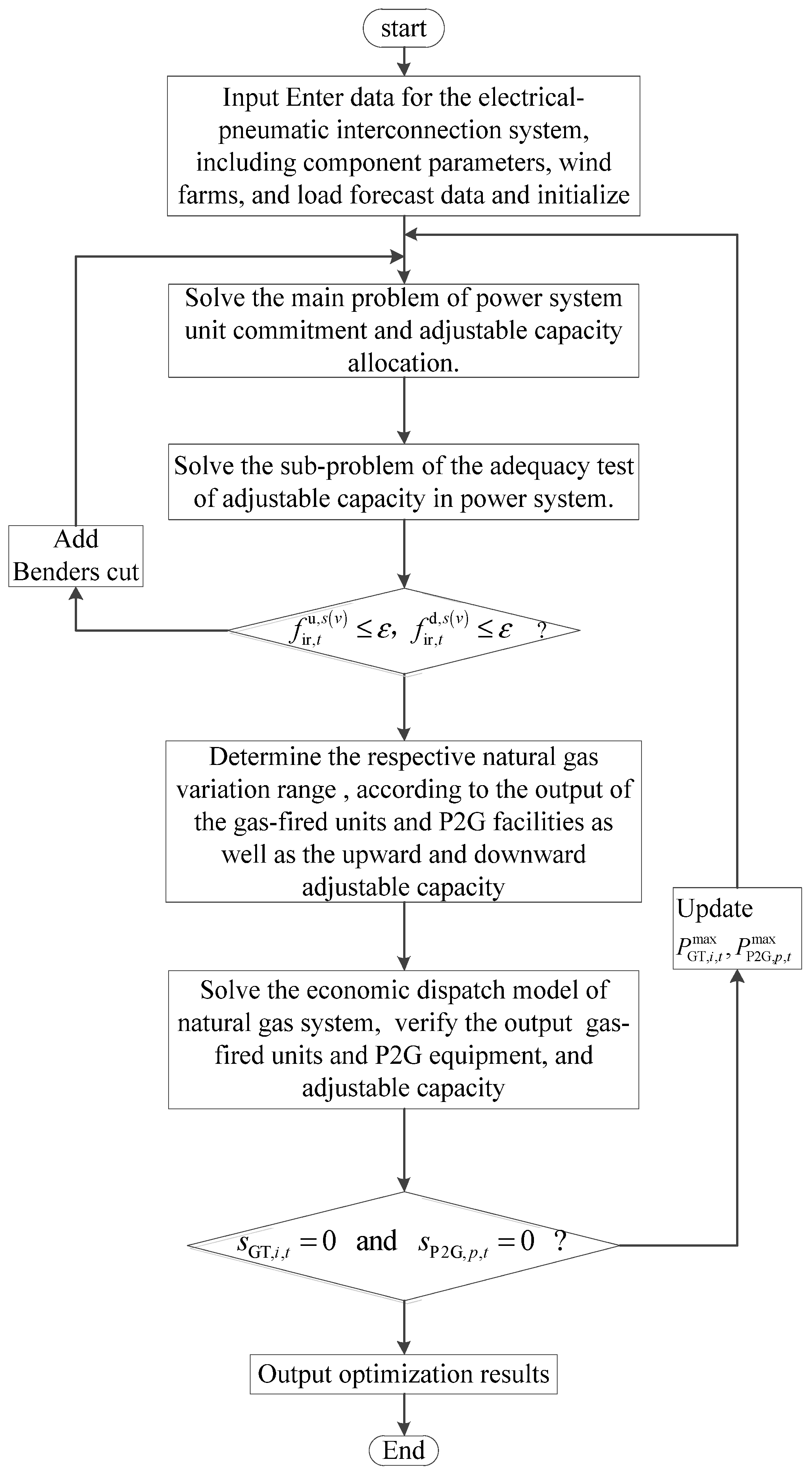
4. Solution Methodology

The flexible economic dispatch model of the IPGS has two sub-problems for optimally dispatching the individual power system and gas system. Furthermore, two sub-problems are coordinated by introducing slack variables to adjust the maximum output of gas-fired units and P2G facilities.

4.1. Flexible Economic Dispatch for the Power System

The flexible dispatching model of the power system is given in Part A, Section III. It belongs to a two-stage mixed integer nonlinear optimization problem. In order to simplify the solution process, this paper first uses a linearization method to deal with the non-linear function and constraints in the model, which are converted into a two-stage mixed integer linear optimization problem. The linearization method has been studied in many papers, so this article will not repeat them. On this basis, the Benders decomposition method is used to iteratively solve the two-stage flexible economic dispatch model. Specifically, for the main problem and the sub-problem, considering that both are linear programming problems after the transformation, the CPLEX commercial solver with high efficiency is directly used for solving.

The optimized solution is obtained through the v-th iteration of the main problem. Mainly the following variables: $f_{\mathrm{g},i,t}^{\mathrm{u}\left(v\right)}$, $f_{\mathrm{g},i,t}^{\mathrm{d}\left(v\right)}$, $f_{\mathrm{dr},m,t}^{\mathrm{u}\left(v\right)}$, $f_{\mathrm{dr},q,t}^{\mathrm{d}\left(v\right)}$, $f_{\mathrm{lcur},b,t}^{\mathrm{u}\left(v\right)}$, $f_{\mathrm{wcur},k,t}^{\mathrm{d}\left(v\right)}$. Bring these results into the sub-problem to obtain the up and down adjustable capacity deficits $f_{\mathrm{ir},t}^{\mathrm{u},s\left(v\right)}$ and $f_{\mathrm{ir},t}^{\mathrm{d},s\left(v\right)}$ in each scenario of the v-th iteration. And judge whether to add Benders cut by (47):

$$f_{\mathrm{ir},t}^{\mathrm{u},s\left(v\right)}\le \epsilon ,f_{\mathrm{ir},t}^{\mathrm{d},s\left(v\right)}\le \epsilon$$

(47)

where $\epsilon$ is a sufficiently small real number. If the adjustable capacity shortages obtained in each scenario satisfy Equation (47), it indicates that the power generation plan and adjustable capacity allocation in the main problem have sufficient flexibility, no Benders cut is generated, and the obtained optimization solution of v-th iteration is the final optimization result. Otherwise, add Benders cut:

$${\displaystyle \sum _{i\in {\mathsf{\Omega }}_{\mathrm{G}}}{\lambda }_{i,t}^{\mathrm{u},s\left(v\right)}\cdot \left(f_{\mathrm{g},i,t}^{\mathrm{u}}-f_{\mathrm{g},i,t}^{\mathrm{u}\left(v\right)}\right)}+{\displaystyle \sum _{m\in {\mathsf{\Omega }}_{\mathrm{DRu}}}{\theta }_{m,t}^{\mathrm{u},s\left(v\right)}\cdot \left(f_{\mathrm{dr},m,t}^{\mathrm{u}}-f_{\mathrm{dr},m,t}^{\mathrm{u}\left(v\right)}\right)}+{\displaystyle \sum _{b\in {\mathsf{\Omega }}_B}{\varsigma }_{b,t}^{\mathrm{u},s\left(v\right)}\cdot \left(f_{\mathrm{lcur},b,t}^{\mathrm{u}}-f_{\mathrm{lcur},b,t}^{u\left(v\right)}\right)}+f_{\mathrm{ir},t}^{\mathrm{u},s\left(v\right)}\le 0$$

(48a)

$${\displaystyle \sum _{i\in {\mathsf{\Omega }}_{\mathrm{G}}}{\lambda }_{i,t}^{\mathrm{d},s\left(v\right)}\cdot \left(f_{\mathrm{g},i,t}^{\mathrm{d}}-f_{\mathrm{g},i,t}^{\mathrm{d}\left(v\right)}\right)}+{\displaystyle \sum _{q\in {\mathsf{\Omega }}_{\mathrm{DRd}}}{\theta }_{q,t}^{\mathrm{d},s\left(v\right)}\cdot \left(f_{\mathrm{dr},q,t}^{\mathrm{d}}-f_{\mathrm{dr},q,t}^{\mathrm{d}\left(v\right)}\right)}+{\displaystyle \sum _{k\in {\mathsf{\Omega }}_{\mathrm{W}}}{\varsigma }_{k,t}^{\mathrm{d},s\left(v\right)}\cdot \left(f_{\mathrm{wcur},k,t}^{\mathrm{d}}-f_{\mathrm{wcur},k,t}^{\mathrm{d}\left(v\right)}\right)}+f_{\mathrm{ir},t}^{\mathrm{d},s\left(v\right)}\le 0$$

(48b)

4.2. Economic Dispatch for the Gas System

The constraints of gas system are all linear constraints except for the pipeline flow equation. To facilitate the computation, the piecewise linear techniques can be employed to linearize the nonlinear parts. At first, take square for both sides of the Equation (38), which gives

$${\tilde{f}}_{ij,t}^2=\mathrm{sgn}\left(p_{i,t},p_{j,t}\right)\cdot {\left(C_{ij}^{gf}\right)}^2\left(p_{i,t}^2-p_{j,t}^2\right)$$

(49)

Then, the big-M method in [35] is adopted to eliminate the sgn(•) function from the equation, giving

$$-M\cdot \left(1-{\nu }_{ij,t}\right)\le p_{i,t}-p_{j,t}\le M\cdot {\nu }_{ij,t}$$

(50)

$$-M\cdot \left(1-{\nu }_{ij,t}\right)\le {\tilde{f}}_{ij,t}^2-{\left(C_{ij}^{gf}\right)}^2\left(p_{i,t}^2-p_{j,t}^2\right)\le M\cdot \left(1-{\nu }_{ij,t}\right)$$

(51)

$$-M\cdot {\nu }_{ij,t}\le -{\tilde{f}}_{ij,t}^2-{\left(C_{ij}^{gf}\right)}^2\left(p_{i,t}^2-p_{j,t}^2\right)\le M\cdot {\nu }_{ij,t}$$

(52)

where ${\nu }_{ij,t}$ is a binary variable and M is a sufficiently large number that can be taken as the maximum value of the pipe flow.

The equivalent pipeline flow equation only contains the nonlinear element of the square term. Therefore, ${\tilde{f}}_{ij,t}^2$, $p_{i,t}^2$ and $p_{j,t}^2$ can be processed by the incremental linearization model with the best calculation efficiency. The specific process can be found in [35].

4.3. Coordinated Optimization of Two Systems

In order to realize the coordination between the two systems, two slack variables $s_{\mathrm{GT},i,t}$ and $s_{\mathsf{P}2\mathsf{G},p,t}$ are introduced to, respectively, represent the infeasible part of gas-fired units consumption and P2G facilities production under the operation constraints of natural gas system.

4.3.1. Slack Variable $s_{\mathrm{GT},i,t}$ for Gas-Fired Units

When the gas system fails to meet the gas demand of gas-fired units, the load shedding will occur and $f_{\mathrm{NL},i,t}$ > 0. Therefore, the slack variable of gas-fired unit can be expressed as follows:

$$s_{\mathrm{GT},i,t}=f_{\mathrm{NL},i,t}$$

(53)

In order to reduce the non-served gas loads of the natural gas system to zero, adjust the maximum output of the gas-fired unit according to the Equation (53) to achieve the coordinated optimization of the two systems.

$$P_{\mathrm{GT},i,t,\max }=h_1^{-1}\left(f_{\mathrm{GT},i,t}-s_{\mathrm{GT},i,t}\right)$$

(54)

where $h_1^{-1}\left(x\right)$ is the inverse of Equation (45).

4.3.2. Slack Variable $s_{\mathsf{P}2\mathsf{G},p,t}$ for P2G Facilities

The slack variable $s_{\mathsf{P}2\mathsf{G},p,t}$ is to ensure that the gas produced by the P2G facility can be fully used by the gas system, so it is calculated according to the following formula:

$$s_{\mathsf{P}2\mathsf{G},p,t}=f_{\mathsf{P}2\mathsf{G},p,t,\max }-f_{\mathsf{P}2\mathsf{G},p,t}$$

(55)

when $s_{\mathsf{P}2\mathsf{G},p,t}$ is greater than zero, adjust the maximum output of P2G facility according to the Equation (56), so that the two systems can achieve coordinated optimization.

$$P_{\mathrm{P}2\mathsf{G},p,t,\max }=h_2^{-1}\left(f_{\mathrm{P}2\mathsf{G},p,t,\max }-s_{\mathrm{P}2\mathsf{G},p,t}\right)$$

(56)

where $h_2^{-1}\left(x\right)$ is the inverse of Equation (46).

Figure 1 shows the flowchart of the proposed bi-level coordinated optimal dispatch of the IPGS. The main steps are as follows:

(1) Solve the main problem of power system unit commitment and adjustable capacity allocation.

(2) Solve the sub-problem of the adequacy test of adjustable capacity in power system.

(3) Check if (47) is satisfied, if not, add Benders cut and return step 1.

(4) According to the output of the gas-fired units and P2G facilities as well as the upward and downward adjustable capacity, the respective natural gas variation range are determined by (45) and (46).

(5) By solving the natural gas system optimal dispatch model, the output of the gas-fired units and P2G facilities as well as the upward and downward adjustable capacity are verified. If both slack variables are zero, the solution is used as an effective solution to the optimization problem of the power system. Otherwise, the maximum output of the gas-fired units and P2G facilities is updated, and the upper power system dispatch model is resolved.

5. Simulation Results

In this work, an IPGS was adopted by a modified IEEE 30-bus power system [36] and a 10-node natural gas system [37] was used to demonstrate the effectiveness of the proposed flexible economic dispatch model and its advantages in enhancing the flexibility and economy of the power system.

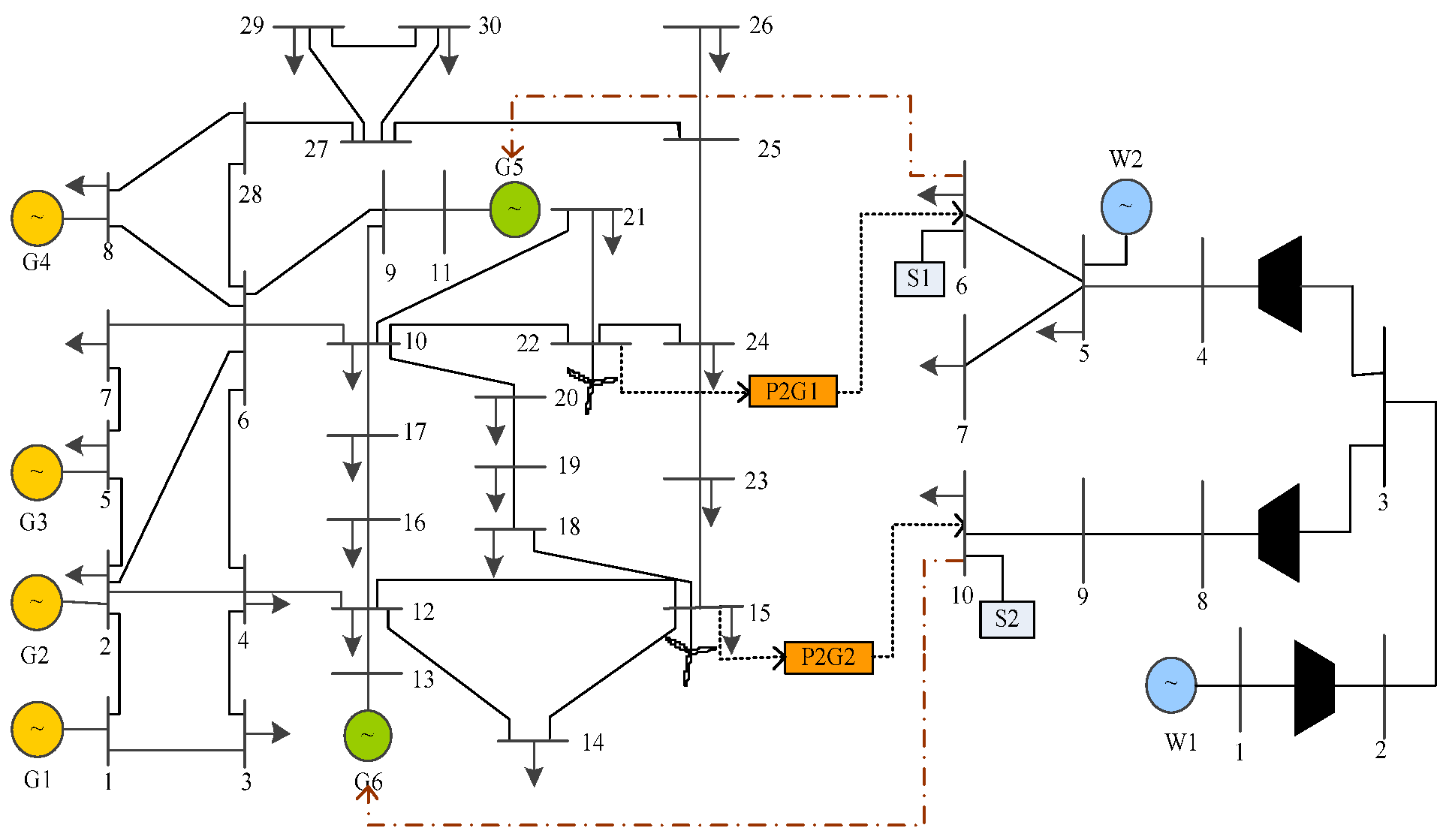
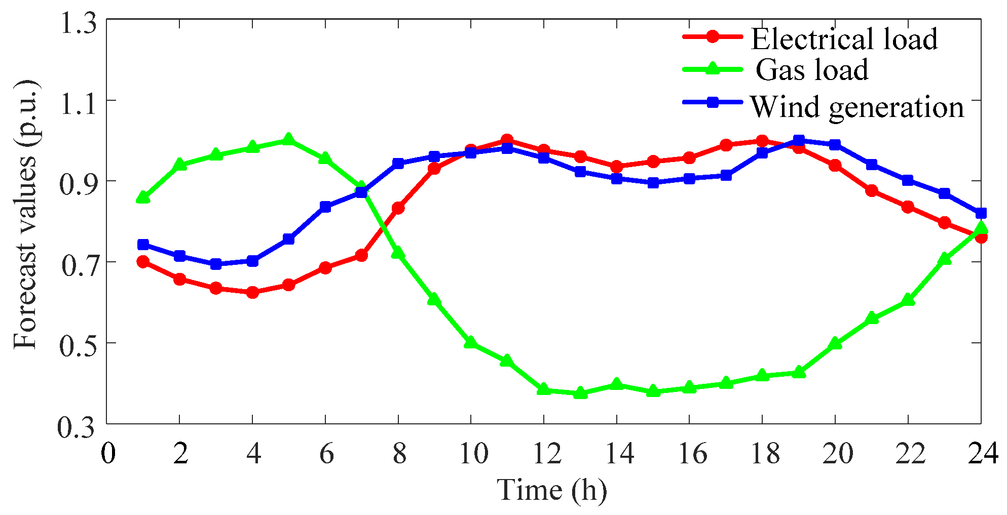
5.1. System Description and Data Source

The topology of the test system is shown in Figure 2 The entire system includes six generating units with a total installed capacity of 540 MW. The main parameters are shown in

Table A1. Parameters of generating units.

Units	Maximum Output (MW)	Minimum Output (MW)	Upward/Downward Ramping Rate (MW·h−1)	Units Type
G1	150	50	65	Coal-fired
G2	130	40	55	Coal-fired
G3	100	35	40	Coal-fired
G4	80	30	35	Coal-fired
G5	40	10	25	Gas-fired
G6	40	10	25	Gas-fired

. The bus 15 and the bus 22 are, respectively, connected to a wind farm with a rated output of 150 MW, and the penalty for wind power curtailment is set at 500 $/(MWh). The gas-fired units G5 and G6 are connected to node 6 and node 10 of the natural gas system respectively. The two P2G facilities are also installed at the bus 22 and bus 15. The maximum/minimum conversion power is 30 MW and 5 MW, and the operating cost is set to 80 $/(MWh). In the gas system, there are two gas wells W1 and W2, two storage facilities S1 and S2, three compressors, six pipelines, and five gas loads. The detailed parameters of the gas sources and storage facilities can be obtained from

Table A2. Parameters of gas wells.

Index	Node No	Min Output (kcf/h)	Max Output (kcf/h)	Gas Price ($/kcf/)
W1	1	2000	8000	1.018
W2	5	1000	3000	1.223

and

Table A3. Parameters of gas storages.

Index	Node No	Max Input (kcf/h)	Max Output (kcf/h)	Capacity (kcf)	Gas Price ($/kcf/)
S1	6	400	300	1000	1.287
S2	10	600	400	1500	1.321

. The P2G operation cost, and penalty cost of not-served gas loads are set as 80 $/(MWh) and 200 $/kcf, respectively. Forecast values of electrical load, gas load and wind generation are shown in Figure 3 with peak values of 504.73 MW, 12,816.52 kcf, and 175.84 MW, respectively.

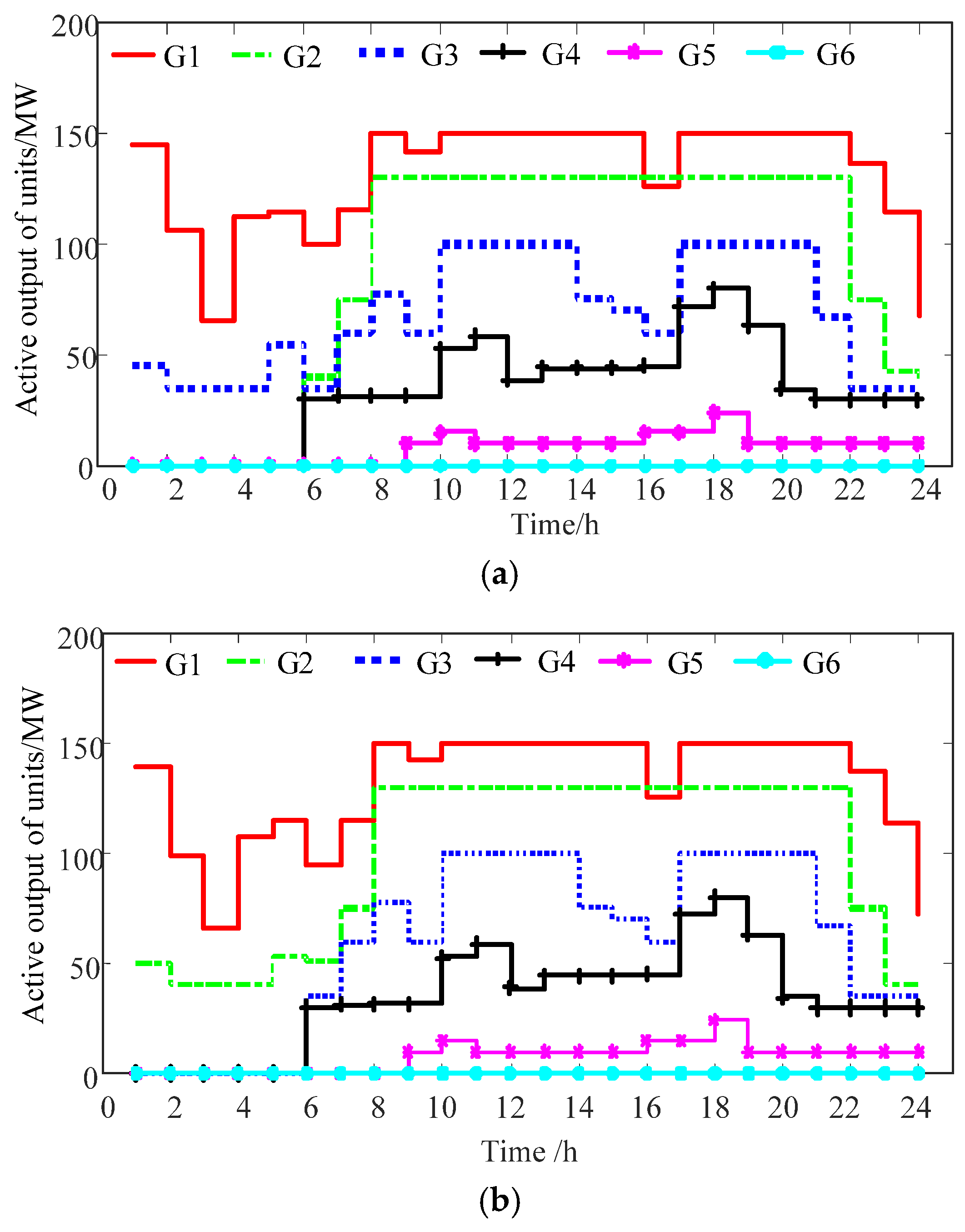
5.2. Analysis of the Impact of P2G on Flexible Economic Dispatch of Power System

The emergence of P2G facilities have made the connection between power systems and natural gas systems increasingly close. At the same time, as the load of the power system, the P2G facilities also provide a new way for the consumption of wind power during the trough of the electrical load, which greatly improves the downward scheduling flexibility and operating economy of the power system.

In order to discuss the impact of P2G facilities on flexible and economical dispatching of the power system, the part on demand response is deleted here, and the following two schemes are set for comparison and analysis:

Case1: Does not include P2G facilities.

Case2: P2G facilities participate in power scheduling and adjustable capacity configuration.

The scheduling results of the power system under the two cases are shown in

Table 1. Dispatch results of power system in two cases.

	Case1	Case2
Units generating cost/$	184,212	183,606
P2G operating costs/$	—	2400
Wind power curtailment cost/$	11,695	0
Load shedding cost/$	7480	7480
Units adjustable capacity allocation cost/$	33,722	33,272
P2G adjustable capacity allocation cost/$	—	500
Total cost/$	237,109	227,259

, and the corresponding unit output curve is shown in Figure 4. And Figure 5 shows the downward adjustable capacity of the power system configuration under the two cases.

It can be seen from Figure 4 that during the trough period of the electric load (1:00–6:00), due to the large wind power output, only the coal-fired units G1 and G3 are in working state in the Case1, and the output is close to the minimum output. The Case1 is similar to the Case2, but considering that the P2G facilities participate in power dispatching and adjustable capacity allocation, they increase the load of the power system during the trough period, and also provide a part of the adjustable capacity for the unit. As a result, in the process of formulating the power generation plan of the units, the coal-fired units G1 and G2 with lower power generation costs are preferentially used to provide power services. Comparing the scheduling results of the two cases in Table 1, it can be found that the generating cost and adjustable capacity allocation cost of the units in Case2 are, respectively, reduced by 606$ and 450$ compared with Case1, which ultimately reduces the total cost of the power system by 4.15%.

Observing Figure 5a, it can be seen that Case1 does not include P2G facilities. During the low load period (1:00–6:00), the system’s downward adjustable capacity is mainly provided by units G1 and G3. Since the adjustable capacity provided by units G1 and G3 cannot meet the fluctuations and randomness of wind power and load. As a result, the downward adjustable capacity of 7.48 MWh and 7.08 MWh was provided to the power system through wind power curtailment at 3:00 and 6:00, respectively. In Figure 5b, Case2 provided 6.96 MW and 6.16 MW of downward adjustable capacity to the power system through the P2G facility during these two periods, so that the wind power curtailment of the power system was reduced to 0.

From the above results, it is not difficult to see that P2G facilities have advantages that cannot be ignored in improving dispatching economy and renewable energy consumption, while providing the system with flexible adjustable capacity. With the large-scale grid integration of wind power, it is necessary to improve the flexibility and economy of the power system through P2G facilities.

5.3. Analysis of Comprehensive Consideration of P2G Facilities and Demand Response

The demand response analysis is further added here, the upward and downward demand response is divided into three levels, and the responsiveness of each level is specified. Bus 4 and Bus 21 access the incentive demand response providers DRu1 and DRu2 to provide upward adjustable capacity, and Bus 7 and Bus 19 access the incentive demand response providers DRd1 and DRd2 to provide downward adjustable capacity. The specific parameters are shown in

Table A4. Parameters of incentive demand response.

Type	Capacity (%)			Price ($/MWh)			RI h	RT h	N times
	1	2	3	1	2	3
DRu1	3	7	9	18	20	22	2	5	3
DRu2	3	5	6	20	22	24	2	4	3
DRd1	3	6	5	21	23	25	2	4	3
DRd2	2	4	3	22	24	26	2	3	3

.

In order to show the advantages of comprehensive consideration of P2G facilities and demand response in improving the flexibility and economy of the power system, the following two cases are also set here for comparative analysis:

Case3: Coordination optimization of IPGS considering only P2G facilities.

Case4: Coordination optimization of IPGS considering P2G facilities and demand response.

Figure 6 shows the output curves of the two cases. Figure 7 shows the upward adjustable capacity of the power system configuration in the two cases.

Comparing the two cases of Figure 6, it can be seen that, during the peak load period, Case4 considers the P2G facilities and demand response to participate in the adjustable capacity configuration, the higher cost gas unit G6 is avoided, and the start time of the gas unit G5 is delayed from 9:00 to 10:00, which plays a role in reducing the number of online generating units and generating costs of generating units.

It can be found in Figure 7 that, in order to meet the upward scheduling flexibility requirements of the power system, Case3 uses gas-fired units with higher configuration costs during peak load hours (10:00–11:00 and 17:00–20:00) to provide adjustable capacity. However, due to the limited adjustable capacity that the unit can provide, at 11:00 it is necessary to provide a 4.30 MW upward adjustable capacity for the power system through load shedding. The Case4 considers demand response and participates in the upward adjustable capacity configuration. Both the adjustable capacity provided by the gas unit G5 at 10:00 and 19:00 and the adjustable capacity provided by the gas unit G6 at 17:00 are changed to demand respond with lower configuration costs, so that the adjustable capacity allocation cost of the power system is effectively improved. More notably, the participation of demand response provided more sources of adjustable capacity for the power system, reducing the adjustable capacity provided by load shedding at 11:00 to 0.17 MW, and optimizing the output of the unit by reducing the adjustable capacity of the G4 unit at 18:00 and 20:00.

It is obvious that, compared with Case3, Case4 considers the demand response and participates in the upward adjustable capacity allocation during the peak load period, which can provide more adjustable capacity sources for the power system, thereby achieving a wider range of optimized resource allocation. Through the coordination between the unit and demand response, it can better cope with the problem of insufficient upward scheduling flexibility of the power system caused by large-scale wind power grid integration.

The various costs of the two cases as shown in

Table 2. Dispatch results of power system in two cases.

	Case3	Case4
Units generating cost/$	190,393	181,665
P2G operating costs/$	2400	1600
Wind power curtailment cost/$	0	0
Load shedding cost/$	4300	170
Units adjustable capacity allocation cost/$	33,295	31,008
P2G adjustable capacity allocation cost/$	687	308
Demand response adjustable capacity Allocation cost/$	—	1398
Total cost/$	231,075	216,151

.

Observing Table 2 and combining the previous flexibility analysis, we find that Case4 considers the demand response and participates in the adjustment of the capacity allocation based on the P2G facilities. The cost of adjustable capacity allocation and the penalty of load shedding are reduced by 2287$ and 4130$ respectively compared to the Case3. At the same time, due to the reduction of the adjustable capacity of the unit configuration, the power system preferentially uses the units with lower power generation costs to provide power services during the formulation of the output plan, which reduces the unit’s power generation costs by 8728$ compared to Case3.

In the end, the total cost of the power system was reduced by 6.45% compared to Case3. It can be seen that comprehensive consideration of P2G facilities and demand response can improve the power system’s scheduling flexibility, while also reducing the power system’s operating costs.

5.4. The Proposed Coordinated Optimization of IPGS

In this part, take Case2 in Part B as an example to compare the individual optimization and coordinated optimization, and analyze the advantages of coordinated optimization in optimizing adjustable capacity allocation and economy.

Figure 8 and Figure 9 show the output of the units and the conversion of active power by the P2G facilities.

Observing Figure 8, it can be found that during the peak load hours (11:00–14:00 and 17:00–20:00), the coal-fired units G1, G2 and G3 with lower power generation costs all operate near the maximum power point, the adjustable upward capacity that can be provided is almost zero. In order to meet the upward scheduling flexibility requirements of the power system during these periods, both scheduling methods have started the gas unit G5 with rapid adjustment capabilities to provide electrical power services. Unlike the separate optimization, however, the coordinated optimization also started the gas unit G6 to participate in power dispatch and adjustable capacity allocation during peak load hours.

It can be seen from Figure 9 that during the period of low power load (1:00–7:00), when the power system is individually optimized, the P2G1 with adjustable capacity allocation and lower cost is preferentially used. While the coordinated optimization, when the natural gas produced by P2G1 cannot be fully utilized, its maximum conversion power is adjusted, so that P2G2 is involved in power scheduling and adjustable capacity allocation from 2:00 to 3:00.

In order to further illustrate the advantages of coordinated optimization in optimizing the adjustable capacity allocation, the upper and lower adjustable capacities of the power system configuration are analyzed. The upward adjustable capacity of the power system configuration under the two scheduling modes is shown in Figure 10.

With reference to Figure 8, it can be seen that during the peak period of electric load (10:00–20:00), the upward adjustable capacity of the power system when independently optimized is mainly provided by the coal-fired power unit G4 and the gas unit G5. As the natural gas system node 6 connected to the gas unit G5 is also in the peak gas consumption period, it is not feasible for G5 to have adjustable capacities of 125.20 kcf, 119.55 kcf, and 123.94 kcf in 11:00, 17:00, and 18:00, respectively. In practice, the power system may experience load reduction during these periods. However, the coordinated optimization reduced the adjustable capacity provided by G5 by starting the gas unit G6 at 16:00, and at the same time increased the upward adjustable space of G4, so that the availability of the adjustable capacity configuration in actual operation was guaranteed. In addition, due to the start-up of the G6 unit, the upward adjustable capacity at 17:00 through load shedding configuration was also reduced from 3.59 MW to 0.

The downward adjustable capacity of the power system configuration under the two scheduling modes is shown in Figure 11.

Based on the analysis of the downward adjustable capacity of the power system configuration under the two scheduling modes in conjunction with Figure 9 and Figure 11, it can be found that during the low load period (1:00–7:00), When individually optimized, the downward adjustable capacity of the power system is mainly provided by the coal-fired power units G1, G2, and P2G1. During the formulation of the scheduling plan, the pressure limit of the natural gas system node 6 and the constraints of the gas intake of the gas storage equipment were not considered. As a result, the natural gas generated by P2G1 was 10.64 kcf and 25.46 kcf at 2:00 and 3:00, respectively, which could not be accepted by the natural gas system. The coordinated optimization adjusts the maximum conversion power of P2G1 in these two periods based on the amount of excess natural gas, so that the downward adjustable capacity provided by P2G1 at 3:00 is changed to be provided by P2G2.

In order to compare the economics, the flexible scheduling costs of the two methods are given, as shown in the

Table 3. Dispatch results of two scheduling modes.

	Separate Optimization	Coordinated Optimization
Units generating cost/$	227,259	190,393
P2G operating costs/$	2400	2400
Wind power curtailment cost/$	0	0
Load shedding cost/$	7480	4300
Units adjustable capacity allocation cost/$	33,272	33,295
P2G adjustable capacity allocation cost/$	500	687
Total cost of power system/$	270,912	231,075
Load reduction of natural gas system/kcf	368	0
Excess natural gas from P2G/kcf	36	0
Total cost of gas system/$	320,656	244,687
Cost of IPGS/$	547,916	475,763

.

From the data in Table 3, it can be seen that under the same scheduling flexibility requirements, when the IPGS is individually optimized, the unit’s generation cost and adjustable capacity allocation cost are lower than the coordinated optimization, and since the natural gas system does not consider the effect of the conversion of active power and adjustable capacity of the P2G facilities, the adjustable capacity allocation cost of the P2G facilities is also reduced by 187$ compared to the coordinated optimization, which ultimately reduces the total cost of the power system by 1.65%. However, it also caused a gas load reduction of 368 kcf during the scheduling process of the natural gas system, which caused the total cost of the natural gas system to increase by 15.16% compared to the coordinated optimization. At the same time, due to the constraints of natural gas system operation constraints, 36 kcf of natural gas generated by the P2G facilities cannot be accepted by the natural gas system. The coordinated optimization of the IPGS reduces the gas load reduction to zero by adjusting the maximum active output of the gas-fired units and the P2G facilities, and the natural gas produced by the P2G facilities is also fully utilized.

From the above data, it can be seen that with the increase of the proportion of gas-fired units, the scheduling scheme based on the constraints of the power system alone cannot give full play to the synergistic effect of the two energy sources. In order to improve the overall resource utilization level of the two energy systems, it is necessary to implement coordinated optimization scheduling.

6. Conclusions

This paper proposes a flexible economic dispatch model under the constraints of power and natural gas systems. To reduce system operation cost and enhance its response capability for uncertainty as much as possible, both the P2G facility and demand response have been considered. The co-optimization model is decomposed into a flexible economic dispatch of upper power system and an economic dispatch of lower natural gas system to realize the distributed co-optimization of power and natural gas system. Moreover, slack variables are introduced for the coordinated optimization of the upper and lower systems. Simulation results demonstrate that the proposed flexible economic dispatch model can improve the power system flexibility better than the economic dispatch model. Considering P2G facilities and demand response at the same time can effectively improve the downward flexibility during the trough period and the upward flexibility during the peak period. Compared with considering the P2G equipment alone, the total operating cost of the electricity-gas system can be reduced by 6.45%. Furthermore, the hourly unit commitment and adjustable capacity of the power system are affected by the natural gas system transmission constraints. The coordinated optimization of the power and natural gas systems can improve the optimal allocation of resources, thus reducing the operation cost of the two systems.

References

1. Han, D.; Li, T.; Feng, S.; Shi, Z. Does Renewable Energy Consumption Successfully Promote the Green Transformation of China’s Industry? Energies 2020, 13, 229. [Google Scholar] [CrossRef] [Green Version]
2. Zhang, Y.; Wang, J.; Ding, T.; Wang, X. Conditional value at risk-based stochastic unit commitment considering the uncertainty of wind power generation. IET Gener. Transm. Distrib. 2018, 12, 482–489. [Google Scholar] [CrossRef]
3. China National Energy Administration. Wind Power Grid-Connected Operation in 2017. 2018. Available online: http://www.nea.gov.cn/2018-02/01/c_136942234.htm (accessed on 1 February 2018).
4. Mohamed, O.; Khalil, A. Progress in Modeling and Control of Gas Turbine Power Generation Systems: A Survey. Energies 2020, 13, 2358. [Google Scholar] [CrossRef]
5. Scheller, F.; Burkhardt, R.; Schwarzeit, R.; McKenna, R.; Bruckner, T. Competition between simultaneous demand-side flexibility options: The case of community electricity storage systems. Appl. Energy 2020, 269, 114969. [Google Scholar] [CrossRef]
6. Clegg, S.; Mancarella, P. Storing renewables in the gas Network: Modelling of power-to-gas seasonal storage flexibility in low–carbonpower systems. IET Gener. Transm. Distrib. 2016, 10, 566–575. [Google Scholar] [CrossRef]
7. Li, Y.; Liu, W.; Shahidehpour, M.; Wen, F.; Wang, K.; Huang, Y. Optimal Operation Strategy for Integrated Natural Gas Generating Unit and Power-to-Gas Conversion Facilities. IEEE Trans. Sustain. Energy 2018, 9, 1870–1879. [Google Scholar] [CrossRef]
8. Faridpak, B.; Farrokhifar, M.; Murzakhanov, I.; Safari, A. A series multi-step approach for operation Co-optimization of integrated power and natural gas systems. Energy 2020, 204, 117897. [Google Scholar] [CrossRef]
9. Farrokhifar, M.; Nie, Y.; Pozo, D. Energy systems planning: A survey on models for integrated power and natural gas networks coordination. Appl. Energy 2020, 262, 114567. [Google Scholar] [CrossRef]
10. Liu, J.; Sun, W.; Yan, J. Effect of P2G on Flexibility in Integrated Power-Natural Gas-Heating Energy Systems with Gas Storage. Energies 2021, 14, 196. [Google Scholar] [CrossRef]
11. Zhang, W.; Liu, R.; Yang, X. Study on Operating Strategy of Electric—Gas Combined System Considering the Improvement of Dispatchability. Energies 2019, 12, 4584. [Google Scholar] [CrossRef] [Green Version]
12. Aldarajee, A.H.M.; Hosseinian, S.H.; Vahidi, B.; Dehghan, S. Security constrained multi-objective bi-directional integrated electricity and natural gas co-expansion planning considering multiple uncertainties of wind energy and system demand. IET Renew. Power Gener. 2020, 14, 1395–1404. [Google Scholar] [CrossRef]
13. He, C.; Wu, L.; Liu, T.; Wei, W.; Wang, C. Co-optimization scheduling of interdependent power and gas systems with electricity and gas uncertainties. Energy 2018, 159, 1003–1015. [Google Scholar] [CrossRef]
14. Zhang, Y.; Huang, Z.; Shu, S.; Zheng, F.; Lin, J. Cooperative Scheduling for Integrated Electricity and Natural Gas Systems Considering Gas Flow Transient Characteristics and Source—Load Uncertainties. Energy Technol. 2020, 8, 201901098. [Google Scholar] [CrossRef]
15. Karamdel, S.; Moghaddam, M.P. Robust expansion co-planning of electricity and natural gas infrastructures for multi energy-hub systems with high penetration of renewable energy sources. IET Renew. Power Gener. 2019, 13, 2287–2297. [Google Scholar] [CrossRef]
16. Fang, X.; Cui, H.; Yuan, H.; Tan, J.; Jiang, T. Distributionally-robust chance constrained and interval optimization for integrated electricity and natural gas systems optimal power flow with wind uncertainties. Appl. Energy 2019, 252, 113420. [Google Scholar] [CrossRef]
17. Chen, J.; Lin, Z.; Ren, J.; Zhang, W.; Zhou, Y.; Zhang, Y. Distributed multi-scenario optimal sizing of integrated electricity and gas system based on ADMM. Int. J. Electr. Power Energy Syst. 2020, 117, 105675. [Google Scholar] [CrossRef]
18. Osi adacz, A.J.; Isoli, N. Multi-Objective Optimization of Gas Pipeline Networks. Energies 2020, 13, 5141. [Google Scholar] [CrossRef]
19. Tan, C.; Geng, S.; Tan, Z.; Wang, G.; Pu, L.; Guo, X. Integrated energy system—Hydrogen natural gas hybrid energy storage system optimization model based on cooperative game under carbon neutrality. J. Energy Storage 2021, 38, 102539. [Google Scholar] [CrossRef]
20. Xi, Y.; Fang, J.; Chen, Z.; Zeng, Q.; Lund, H. Optimal coordination of flexible resources in the gas-heat-electricity integrated energy system. Energy 2021, 223, 119729. [Google Scholar] [CrossRef]
21. Zhang, B.; Hu, W.; Cao, D.; Huang, Q.; Chen, Z.; Blaabjerg, F. Economical operation strategy of an integrated energy system with wind power and power to gas technology—A DRL-based approach. IET Renew. Power Gener. 2021, 14, 3292–3299. [Google Scholar] [CrossRef]
22. Wang, S.; Yuan, S. Interval optimization for integrated electrical and natural-gas systems with power to gas considering uncertainties. Int. J. Electr. Power Energy Syst. 2020, 119, 105906. [Google Scholar] [CrossRef]
23. Chen, Z.; Zhang, Y.; Ji, T.; Li, C.; Xu, Z.; Cai, Z. Economic dispatch model for wind power integrated system considering the dispatchability of power to gas. IET Gener. Transm. Distrib. 2019, 13, 1535–1544. [Google Scholar] [CrossRef]
24. Liu, J.; Sun, W.; Harrison, G.P. The economic and environmental impact of power to hydrogen/power to methane facilities on hybrid power-natural gas energy systems. Int. J. Hydrog. Energy 2020, 45, 20200–20209. [Google Scholar] [CrossRef]
25. Zhang, Y.; Huang, Z.; Zheng, F.; Zhou, R.; An, X.; Li, Y. Interval optimization based coordination scheduling of gas—Electricity coupled system considering wind power uncertainty, dynamic process of natural gas flow and demand response management. Energy Rep. 2020, 6, 216–227. [Google Scholar] [CrossRef]
26. Li, P.; Wang, Z.; Wang, J.; Yang, W.; Guo, T.; Yin, Y. Two-stage optimal operation of integrated energy system considering multiple uncertainties and integrated demand response. Energy 2021, 225, 120256. [Google Scholar] [CrossRef]
27. Kou, X.; Li, F.; Dong, J.; Starke, M.; Munk, J.; Xue, Y.; Olama, M.; Zandi, H. A Scalable and Distributed Algorithm for Managing Residential Demand Response Programs using Alternating Direction Method of Multipliers (ADMM). IEEE Trans. Smart Grid 2020, 11, 4871–4882. [Google Scholar] [CrossRef]
28. He, C.; Zhang, X.; Liu, T.; Wu, L. Distributionally Robust Scheduling of Integrated Gas-Electricity Systems with Demand Response. IEEE Trans. Power Syst. 2019, 34, 3791–3803. [Google Scholar] [CrossRef]
29. Rakipour, D.; Barati, H. Probabilistic optimization in operation of energy hub with participation of renewable energy resources and demand response. Energy 2019, 173, 384–399. [Google Scholar] [CrossRef]
30. Subramanya, K.; Nagaraj, M.S. Optimization of Demand Side Management and DG Placement in the Distribution System with Demand Response. Int. J. Eng. Adv. Technol. 2020, 10, 407–414. [Google Scholar]
31. Wang, C.; Chen, S.; Mei, S.; Chen, R.; Yu, H. Optimal Scheduling for Integrated Energy System Considering Scheduling Elasticity of Electric and Thermal Loads. IEEE Access 2020, 8, 202933–202945. [Google Scholar] [CrossRef]
32. Ming, H.; Xie, L.; Campi, M.C.; Garatti, S.; Kumar, P.R. Scenario-Based Economic Dispatch with Uncertain Demand Response. IEEE Trans. Smart Grid 2019, 10, 1858–1868. [Google Scholar] [CrossRef] [Green Version]
33. Ju, L.; Tan, Z.; Yuan, J.; Tan, Q.; Li, H.; Dong, F. A bi-level stochastic scheduling optimization model for a virtual power plant connected to a wind–photovoltaic–energy storage system considering the uncertainty and demand response. Appl. Energy. 2016, 171, 184–199. [Google Scholar] [CrossRef] [Green Version]
34. Wang, C.; Wang, Z.; Hou, Y.; Ma, K. Dynamic game-based maintenance scheduling of integrated electric and natural gas grids with a bilevel approach. IEEE Trans. Power Syst. 2018, 33, 4958–4971. [Google Scholar] [CrossRef] [Green Version]
35. He, C.; Wu, L.; Liu, T.; Shahidehpour, M. Robust co-optimization scheduling of electricity and natural gas systems via ADMM. IEEE Trans. Sustain. Energy 2017, 8, 658–670. [Google Scholar] [CrossRef]
36. Power System Test Case Archive. Available online: http://labs.ece.uw.edu/pstca (accessed on 30 August 1993).
37. Wu, S.; Rios-Mercado, R.Z.; Boyd, E.A.; Scott, L.R. Model relaxations for the fuel cost minimization of steady-state gas pipeline networks. Math. Comput. Model. 2000, 31, 197–220. [Google Scholar] [CrossRef]
Figure 1. Flowchart of the model solution.
Energies 14 05554 g001
Figure 2. Structure of integrated power and gas systems.
Energies 14 05554 g002
Figure 3. Forecast values of electrical load, gas load and wind generation.
Energies 14 05554 g003
Figure 4. Power output of units in different Cases: (a) Case 1; (b) Case 2.
Energies 14 05554 g004
Figure 5. Power system downward adjustable capacity in different Cases: (a) Case1 and (b) Case2.
Energies 14 05554 g005aEnergies 14 05554 g005b
Figure 6. Power output of units in different Cases: (a) Case3; (b) Case4.
Energies 14 05554 g006
Figure 7. Power system upward adjustable capacity in different Cases: (a) Case3; (b) Case4.
Energies 14 05554 g007
Figure 8. Power output of units in different dispatch modes: (a) Separate optimization and (b) coordinated optimization.
Energies 14 05554 g008
Figure 9. Power converted by P2G facilities in different dispatch modes: (a) Separate optimization and (b) coordinated optimization.
Energies 14 05554 g009
Figure 10. Power system upward adjustable capacity in different dispatch modes: (a) Separate optimization and (b) Coordinated optimization.
Energies 14 05554 g010aEnergies 14 05554 g010b
Figure 11. Power system downward adjustable capacity in different dispatch modes: (a) Separate optimization and (b) coordinated optimization.
Energies 14 05554 g011