Abstract
Magnetohydrodynamic (MHD) phenomena, due to the interaction between a magnetic field and a moving electro-conductive fluid, are crucial for the design of magnetic-confinement fusion reactors and, specifically, for the design of the breeding blanket concepts that adopt liquid metals (LMs) as working fluids. Computational tools are employed to lead fusion-relevant physical analysis, but a dedicated MHD code able to simulate all the phenomena involved in a blanket is still not available and there is a dearth of systems code featuring MHD modelling capabilities. In this paper, models to predict both 2D and 3D MHD pressure drop, derived by experimental and numerical works, have been implemented in the thermal-hydraulic system code RELAP5/MOD3.3 (RELAP5). The verification and validation procedure of the MHD module involves the comparison of the results obtained by the code with those of direct numerical simulation tools and data obtained by experimental works. As relevant examples, RELAP5 is used to recreate the results obtained by the analysis of two test blanket modules: Lithium Lead Ceramic Breeder and Helium-Cooled Lithium Lead. The novel MHD subroutines are proven reliable in the prediction of the pressure drop for both simple and complex geometries related to LM circuits at high magnetic field intensity (error range %).
1. Introduction
The Breeding Blanket (BB) is a crucial component in the project of magnetic-confinement nuclear fusion reactors. The BB carries out three main functions: it conveys the heat produced by the plasma to the primary cooling system of the reactor, provides radiation shielding for personnel and components and produces enough tritium to ensure the fuel self-sufficiency of the reactor. Several blanket design solutions have been proposed where liquid metals (LMs), such as Lithium (Li) or Lithium–Lead alloys (Li-Pb), are used as working fluids [1]. One of the critical issues in the project of a LM blanket is represented by magnetohydrodynamic (MHD) phenomena that occur in the piping network of the blanket [2]. MHD effects are due to the interaction between the flowing liquid metal, that is an electro-conductive material, with the high magnetic field employed to confine the plasma in the reactor chamber. Electrical currents are induced in the conductive fluid volume and, in turn, Lorentz forces are generated, altering the flow behaviour compared with the ordinary hydrodynamic (OHD) case. For instance, MHD phenomena modify the velocity distribution and mass transport inside the ducts, enhance pressure losses, affect heat transfer mechanisms, etc. Estimating the impact of all those effects on the component performance is essential for an efficient project of a liquid metal breeding blanket and, therefore, the development of numerical tools able to predict them is extremely desirable [3]. An extensive overview of MHD phenomena that affect the BB design is available in Ref. [4].
In this work, the analysis is focused on the additional pressure drops introduced by the electromagnetic drag. Generally, it is possible to assume that MHD pressure losses are composed by the sum of two terms [5]:
In Equation (1), the first right-hand term () quantifies the pressure losses due to Lorentz forces opposite to flow direction, induced by electrical currents that are confined in a plane perpendicular to fluid velocity. Two-dimensional MHD pressure drop is the only term driving the head loss in a fully developed flow configuration, i.e., in straight conduits. The second right-hand term () stands for the contribution of not “cross-sectional” currents (three-dimensional currents) that, interacting with the magnetic field, produce Lorentz forces in other direction than the stream one. Three-dimensional currents arise whenever axial electric potentials are induced within the fluid body either due to the channel complex geometry (cross-section variation, change of stream direction, etc.), or non-uniform electromagnetic boundary conditions, may that be a discontinuity of wall conductivity or a strong magnetic field gradient [6]. Formally, the total head loss () in a closed system is composed by the sum of the hydrodynamic pressure drop, caused by distributed and concentrated friction losses, and the overall MHD loss due to the electromagnetic drag:
Considering the typical magnitude of the magnetic field encountered in fusion reactors (≈4–9 T), it can be demonstrated that the pressure drop due to MHD phenomena are dominating the other contribution, so that . For instance, the MHD pressure loss in the Li-Pb loop of the European Demonstrator Reactor Water-Cooled Lithium Lead (EU DEMO WCLL) is estimated at ≈1.5 and ≈2.5 MPa for the outboard and inboard segment, whereas the OHD loss does not exceed 0.1 MPa [7].
The flow path of the liquid metal in the piping system of a blanket comprises a multitude of complex elements, such as manifolds and junctions, alongside with straight ducts. Hence, in the pressure drop assessment in a BB, both contributions of 2D and 3D MHD pressure loss must be taken into account. Generally, blanket-scale analyses for MHD phenomena are performed adopting a semi-analytical approach, in which empirical and semi-empirical correlations are supplemented with data extrapolated by direct numerical simulations [5,7,8]. This methodology, although effective to a certain degree, happens to be extremely time-consuming, not flexible in its scope, and with serious limitations in the achievable spatial and temporal resolution. Several computational fluid dynamic (CFD) tools have dedicated MHD modules, such as ANSYS-CFX, ANSYS-FLUENT and OpenFOAM but a comprehensive and mature code able to simulate all the MHD phenomena in the blanket is not yet available [9]. Unfortunately, reactor-scale analysis is not possible with CFD codes and, in any case, will be prohibitive in terms of calculation time and computational effort. Conversely, best-estimate systems thermal-hydraulic (BE SYS-TH) codes could enable the efficient and quick simulation of the blanket piping network level but, currently, they have limited or non-existent MHD capability.
This kind of codes are crucial for the assessment of thermal-hydraulics phenomena occurring within complex nuclear systems. BE codes are mainly developed for the analysis of incidental or accidental transients but are also employed for the characterization of operational transients or steady-states configurations [10]. Generally, to compute the underlying physics in such challenging scenarios, SYS-TH tools use 0-D or 1-D models derived by the analysis of numerous experimental campaigns. They are often used for safety demonstration analyses and BE SYS-TH codes are considered the reference numerical tools for the licensing of fission nuclear power plants [11]. A typical example of SYS-TH code is RELAP5 that, despite being initially developed for applications in light water reactors, has been extended in recent years to employ other fluids (i.e., liquid metals, molten salts, etc.). Rudimentary MHD correlations are implemented in RELAP5-3D [12] and MARS-FR [13] but are limited to straight rectangular/circular ducts and, thus, do not support any treatment for junctions, manifolds, etc. Basic MHD modelling capabilities have been implemented in MELCOR 1.8.5 and 1.8.6, which have been modified for the study of fusion-relevant systems [14,15,16]. Moreover, pursuing the quest for the realization of a MHD system-level tool, a novel code called MHD-SYS has been developed that features models for the simulation of multiple electrical-coupled ducts and heat transfer for basic layouts, whereas coupling with CFD codes is employed to supply the system code with reliable input data for the behaviour of the flow in complex geometrical elements [17]. The coupled approach for component-level analysis, although somewhat effective, nullifies the main benefit of a stand-alone BE code, hampering its agile functioning. More recently, basic MHD features have been implemented in GETTHEM, a tool developed specifically for tokamak fusion reactors, to model pressure drops in the WCLL Li-Pb loop [18,19].
The aim of this work is to present the first phase of the development of a comprehensive and robust numerical tool able to handle all the fundamental MHD effects occurring in a LM breeding blanket, ranging from pressure loss to mass transport, in order to support fusion reactor design. It is important to underline that at this early stage, attention will be focused on MHD features that influence the nominal operation of the reactor and for which the state of the knowledge is deemed sufficient to support the implementation of a SYS-TH module. MHD impact on relevant accidental transients for the BB (for instance, how an anticipated accidental pressure transient is affected by the tokamak magnetic field) is still under discussion and, as such, it will be taken into account once more data become available.
The prediction of the MHD pressure drop is one of the main concerns for liquid metal BB design and has been given priority in the code implementation. In the following, we discuss the models that, derived by experimental and numerical works, have been included in the system code RELAP5/MOD3.3. A verification and validation (V&V) procedure is reported to assess the confidence of our numerical method against the benchmark of high-quality numerical simulations and experimental data, as suggested by Ref. [20].
2. MHD Formulation
The incompressible electrically conducting fluid flow, under the influence of a magnetic field, is properly described by the combination of Navier–Stokes and Maxwell equations. For liquid metal flows in fusion reactor loops, the induction-less or low magnetic Reynolds number approximation is allowed, so that the self-induced magnetic field effect is neglected, and the velocity/magnetic field coupling is simplified reducing the latter to a boundary condition of the problem [21]. For the scope of this study, it is useful to focus our attention on the coupled momentum balance equation in its nondimensional form:
In Equation (3), vectors v, j and B stand for velocity, current density and magnetic field, respectively, and p is the pressure. They are made nondimensional by scaling with the mean velocity , and the external magnetic field magnitude ; the nondimensional pressure p is scaled through the value .
Parameter a stands for the typical length scale for the specific case of study (i.e., half-length of a duct along magnetic field direction), whereas is the electrical conductivity of the fluid. The flow is governed by two fundamental parameters: the Hartmann number () and the Stuart number, or interaction parameter (N).
The square of sets the ratio of electromagnetic to viscous forces, whereas N gives the ratio of electromagnetic to inertial forces. Symbols and denote dynamic viscosity and density of the fluid, respectively. Those parameters may be combined to return the Reynolds number () in its classical formulation:
In LM loops for blanket applications, and N reach very high values (≈, [5]), so that MHD flows can be approximated as viscous-less and inertia-less in most cases. Therefore, in the core region of fluid domain, the motion is governed by the balance between Lorentz and pressure force, whereas inertial and viscous effects are confined in thin fluid layers of thickness O() and O() close to solid walls perpendicular or parallel to the magnetic field direction [21].
Another fundamental nondimensional parameter must be defined to represent the tendency of the induced currents to close either through the fluid or the bounding walls. The pipe system that hosts the liquid metal, generally, is itself made of electro-conductive material. Thus, electric currents arising in the fluid tend to close their path through the electrically conducting duct walls. Moreover, if different channels have common walls, they may interact by exchanging electric currents across those walls. This effect is known as Madarame effect or electromagnetic coupling [22]. The wall conductivity is usually expressed through the wall conductance ratio, c:
where and are the electrical conductivity of the duct walls and their thickness.
Magnetohydrodynamic pressure drops in liquid metal circuits depend on all parameters discussed above. As already pointed in Section 1, 2D MHD pressure drop can be considered as the analogue of hydrodynamic friction loss (also referred as distributed head loss). It is the “electromagnetic drag” that dissipates fluid kinetic energy via Joule effect. This phenomenon has been studied in-depth hence its characterization can rely on an exhaustive amount of data. Therefore, extensively validated correlations are available in the literature for fully developed magneto-hydraulic loss of load [6,23,24]. Nevertheless, it is crucial to underline that the current version of RELAP5 can model only ducts which are assumed to be immersed in a dielectric medium, i.e., air. This assumption is not usually verified in a reactor where, unless the liquid metal is insulated from the structural material through some technical means, the conduits are in electrical contact with each other. Theoretical understanding of electromagnetic coupling is still limited; it is not possible, at this stage, to develop a suitable system code model to account for its effect (i.e., altered pressure loss and flow distribution). However, the above-mentioned assumption, although portraying a simplified picture, is still useful to predict pressure loss figures that are representative of the behaviour of a more realistic system, as it is demonstrated in Section 4.
Three-dimensional pressure losses, instead, can be treated as the MHD analogue of hydrodynamic localized losses. They are caused by electrical current closing their paths in stream-wise direction, that arise whenever the flow meets complex geometries (such as bends, cross-section variations, obstacles), different walls electrical conductivity and non-uniform magnetic field. All those are common features in the liquid metal piping network of a fusion reactor. However, data for 3D MHD pressure losses are relatively scarce compared with these available for fully developed MHD flow. Evaluating those kinds of losses is much more challenging since they strongly depend on the flow geometry and governing parameters. For these reasons, only configurations that have been studied and characterized the most are taken into account: expanding/contracting pipes, bending conduits and ducts with discontinuities in the conductance ratio (Flow Channel Inserts). In other words, the current RELAP5/MOD3.3 implementation for MHD 3D models has been devised as a readily extendable framework, which is amenable to be improved as soon as the knowledge progresses in this field. We anticipate revising the code implementation in the next years to increase its level of detail and accuracy.
3. RELAP5/MOD3.3 Overview and Models
RELAP5/MOD3.3 (referred as RELAP5 in the following) is a 1D thermo-hydraulic code, developed in Fortran language, that is based on a non-homogeneous and non-equilibrium model for the two-phase (liquid-vapour) system that is solved by a partially implicit numerical scheme to permit fast calculation of system transients. In particular, for the basic hydrodynamic model, which is solved numerically using a semi-implicit finite-difference technique, the two-fluid momentum equations are formulated in terms of volume and time-averaged parameters of the flow. Phenomena that are described by non-axial gradients, such as friction losses or heat transfer, are modelled in terms of fluids bulk properties employing empirically-derived transfer coefficient correlations [25].
RELAP5 has been developed for BE transient simulations of light water reactor coolant systems during postulated accidents. The code models the coupled behaviour of the reactor coolant system and the core for loss-of-coolant accidents and operational transients. A generic modelling approach is used that permits simulating a variety of thermal-hydraulic systems [25].
As such, RELAP5 has been extensively validated for a wide range of fission reactor applications and it is regarded as the “gold standard” for those activities. For those reasons, it is considered the best candidate to be improved and modified to become an essential instrument for fusion reactor design. Magnetohydrodynamic features are not implemented in the original version of the code since liquid metal MHD is not relevant to the design of fission reactors.
All the modifications for including magnetohydrodynamic effects on pressure drop are performed starting from an enhanced version of the RELAP5 system code [26,27,28]. This version was developed at the Department of Astronautical, Electrical and Energy Engineering (DIAEE) of “Sapienza” University of Rome in collaboration with ENEA, following a similar approach of other previous versions developed by ENEA and University of Pisa for liquid metals, in which the modelling capability for fusion reactors and their primary cooling systems is enhanced [29]. In this version of the code, updated physical properties for Li-Pb and sodium-potassium (NaK) liquid metals are implemented. These metals are used in this paper for the validation and verification of the MHD model. This choice is made because Li-Pb happens to be the most promising alloy (as coolant and/or breeder) for fusion reactors [30,31]; NaK, on the other hand, is extensively used as model fluid in experimental campaigns for the analysis of magnetohydrodynamic phenomena [32,33,34]. Other breeder fluids of interest, like the FLiBe molten salt, could be implemented in the future. Thermo-physical properties for those materials are inserted in the code following the approach employed in [35] for lead (Pb) and lead-bismuth (LBE) properties. For lithium-lead properties, the work performed by Martelli et al. is taken as reference [36], whereas the one developed by Foust is employed for sodium-potassium [37].
Moreover, electrical conductivity calculation for these and other relevant structural materials (Eurofer97, stainless steel, alumina, etc.) is currently performed by RELAP5 through a new specific subroutine. However, solid wall electrical conductivity is automatically calculated for Eurofer97 only, from the correlation outlined by Mergia and Boukos in [38]. For the analysis presented in this paper, whenever the input wall material needs to be different from the latter, the source code is changed. In a further release, this procedure is foreseen to be automated, alongside with extending the database of ducts wall materials to other commonly encountered in fusion blanket design: vanadium alloys, Inconel steels, alumina, silicon carbide composite, etc. In Table 1, the electrical conductivities for relevant materials in the framework of this activity are reported.

Table 1.
Electrical conductivity for different materials. (*) Temperature T in K. (**) Temperature T in °C.
The program takes in account magnetohydrodynamic effects by computing two different factors: one related to friction losses and cross-sectional currents (2D friction factor), and the other one considered as a local loss factor (3D coefficient) caused by the induction of axial currents [2]. Each factor is calculated by different subroutines that are called whenever a liquid metal is defined in input. The implementation is designed to sum MHD pressure loss factors with the hydrodynamic ones, either for distributed () or local () pressure drops, as is shown in Equation (8), which represents the basic differential one-dimensional single-phase (liquid) formulation adopted for momentum conservation, where stands for liquid volume fraction and the term takes in account body forces effects. As reasonable, the ordinary behaviour is recovered when the magnetic field is set to zero.
Exclusively liquid-phase equations are affected by MHD phenomena, no attempt has been made to develop a multi-phase MHD model. This choice is justified since only sub-cooled liquid metal flows are considered relevant for near-term fusion applications and helium bubble formation in the breeder, albeit important locally is not expected to change its overall behaviour. At last, it is worth underlining that, during the whole implementation campaign, compatibility tests (involving steam/liquid water) have been carried out and it has been verified that the new routines do not affect the original capabilities of the code, whenever they are not called.
3.1. 2D Magnetohydrodynamic Pressure Drop Factor
MHD pressure drops due to cross-sectional currents are modelled in the code adding a coefficient () to the hydrodynamic friction factor computed by RELAP5 to estimate the hydraulic head loss:
MHD pressure drop factor for 2D effects is implemented considering the magnetic field as uniform, transverse to the flow direction and aligned with at least a pair of duct walls (see Figure 1). Furthermore, viscous forces are always supposed negligible, namely . Under those assumptions, MHD pressure loss in a straight channel can be evaluated according to Equation (9) where v is the average fluid velocity and x is the axial length direction of the component.
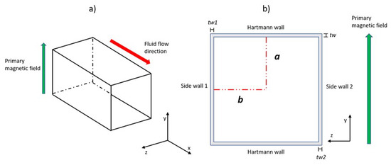
Figure 1.
(a) Three-dimensional view of a generic hydraulic element (single volume). The green vector is the magnetic field applied and is considered perpendicular with respect to the fluid stream direction (red arrow). (b) Cross-sectional view of a hydraulic element. Walls perpendicular to the magnetic field are called Hartmann walls, while those aligned to the magnetic field are referred as Side walls. Characteristic lengths of the component a and b are underlined, and thickness of the walls () as well.
The factor is a function of channel shape, geometry parameters and fluid/walls material. For square/rectangular cross-section conduits, it is derived from engineering correlations reported by Kirillov et al. [6] and it is expressed as:
In Equation (10), c is the wall conductance ratio of the Hartmann walls (walls perpendicular to B, see Figure 1b), and are the wall conductance ratio for the side walls (walls parallel to B); all these quantities are calculated with Equation (7). The symbol stands for the channel aspect ratio, where b is the channel half-width perpendicular to the magnetic field. This correlation has been developed for ducts that may have different walls thickness or, equivalently, non-uniform wall conductance ratio (), that is a common feature in liquid metal circuits. It is valid only for channels that have a uniform Hartmann wall conductivity (c). For duct geometries that cannot be treated with this approach, the wall with the highest conductive ratio should be conservatively assumed to be representative of the whole channel.
If the duct walls have a uniform thickness, Equation (10) can be simplified [6,23,24]:
Similarly, a conduit with circular cross section and uniform wall conductivity is treated with another simplified expression of Equation (10) [6,23,24]:
It is important to keep in mind that predictions from Equations (10)–(12) show slight deviation from experimental data (i.e., ), according to the overview provided by Tassone et al. in [5]. In Table 2, all parameters needed for computation are collected. Electrical conductivity, in , for both fluid () and walls material () are computed by the code.
Table 2.
Parameters used to compute Magnetohydrodynamic 2D additional pressure drop factor.
3.2. 3D Magnetohydrodynamic Pressure Drop Factor
Magnetohydrodynamic local pressure drop factor (3D) is computed by the code when it detects between two hydraulic elements a difference of: cross section, stream direction or electrical conductivity. The local factor represents the 3D effects caused by the induction of axial currents and it is nondimensional. Three-dimensional pressure drops are calculated according to Equation (13) [4,5]:
where is the fluid density, dependent by the temperature, and v is the average fluid velocity. Furthermore, is the sum of three separate K factors, each one representative of a single condition that causes the appearance of 3D MHD pressure losses.
In Equation (14), is the factor correlated to cross section variation, is the one referred to change of stream direction, and is the coefficient that takes into account pressure drop when there is a large difference in electrical conductance between two components.
3.2.1. Bends
Correlations for , to evaluate MHD pressure drop in bends (Figure 2a), are derived mainly referring to Kirillov et al. [6] for circular pipes () and Reimann experimental study [39] for square conduits ().
Equation (15) is conceived for bend pressure drop in insulated circular channels, therefore is considered suitable also for electro-conductive ones, being conservative. Conversely, Equation (16) is derived for bends in square/rectangular ducts. However, assuming an inertia-less flow, they both can be used for any curvature angle (, expressed in degrees) via the correction factor . This means that, for example, a curve can be treated as the composition of two following bends. Previous studies have analysed the case of a bend in the flow path occurring in a plane parallel or perpendicular to the magnetic field direction. It is known that pressure loss associated with a bend perpendicular to the magnetic field direction () is always smaller (if not negligible) compared with the same case featuring a parallel magnetic field () [6]. The underlying physics of such behaviour is quite complex, however, a qualitative explanation is offered in the following. In a MHD flow, the magnetic field tends to dampen the angular momentum components that are not parallel to the field itself. Therefore, liquid sub-structures (e.g., vortexes) that own an angular momentum which is preferentially perpendicular to B are rapidly dissipated, at the expense of the overall energy of the fluid. Only the angular momentum parallel to the field is preserved [40]. When the fluid is forced to bend in a direction the angular momentum is mostly aligned with the field, thus, a relatively low amount of energy will be lost to rearrange the liquid sub-structures. Conversely, when the flow meets a alterations along its path the angular momentum of the fluid will be preferentially perpendicular to the magnetic field and consequently a substantial loss of energy will occur to establish again fully developed conditions.
Correlations (15) and (16), originally developed for this latter case, are adapted to perpendicular bends by adopting a scaling factor [5]. Such corrective factor has been arbitrarily chosen to take in account the minor impact that bends have on the overall loss of load if compared with bends. This formulation has been proven reasonably reliable for modelling complex piping systems involving bending conduits, as discussed in the following (i.e., Secetion Section 4). When more data will be available in the literature, which is currently lacking comparative analysis for those configurations, it is planned to reassess the scale in the interest of a better fidelity to physical behaviour. and are shown in Equations (17) and (18), respectively.
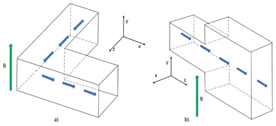
Figure 2.
Geometry configurations examples that can be modelled with the new features implemented in the code. With the green vector is pointed the external magnetic field, B. (a) Bending square pipe geometry, with bending plane perpendicular to the magnetic field direction. (b) Square-to-rectangular duct expansion along B direction.
Therefore, RELAP5 is currently able to treat and bends for any curvature ratio and angle.
3.2.2. Sudden Cross-Section Variations
The model for the calculation of MHD local pressure loss coefficient () caused by the variation of the cross section between two volumes is developed on the basis of the experimental work led by Bühler and Horanyi described in [32].
They considered the case of a rectangular duct undergoing a sudden cross-section expansion parallel to the magnetic field direction (see Figure 2b) and developed an empirical correlation to predict the 3D pressure drop, reported in a simplified form below:
In essence, the pressure drop introduced by expansion geometry is the sum of three contributions: is a term derived by an asymptotic analysis for and , whereas terms and assess the influence of viscous effects and inertial phenomena. Equation (19) is valid for and expansion ratio (formally, the ratio between the characteristic length of the downstream duct and upstream one), which were used during the experimental campaign. Nevertheless, starting from Equation (19), the model has been extended to cover a wider range of expansion ratios and contraction ratios. The model for relies on the assumption that expansions and contractions can be considered as reversible configurations (an expansion, if the flow through it is reversed, became a contraction or vice versa), hence they yield the same pressure drop when the expansion ratio and the contraction ratio are inverse. This is strictly true only for a flow where inertial effects are negligible . In other words, is supposed symmetrical with respect to the cross-section variation ratio. Furthermore, an upper limit value is imposed for the local MHD factor. As matter of fact, according to the numerical analysis led by Feng et al. [41], the additional pressure drop caused by expansion ratio higher than 8 is independent by . Hence, a maximum , as suggested by Smolentsev et al. in [4], is assumed. At last, for simulating cross-section variations occurring perpendicular to B (), a conservative scaling factor is employed, following the same approach discussed for bends (see Section 3.2.1).
The model is currently able to treat for B parallel and perpendicular to the cross-section variation. The influence of wall conductivity and cross-section shape on the 3D loss is not currently implemented and this issue is planned to be addressed in the future, considering as starting point the numerical analysis performed by Rhodes et al. in [42], dealing with an electrically insulated sudden expansion.
3.2.3. Flow Channel Inserts
For discontinuity in wall electrical conductivity, the correlations implemented for are extracted from experimental and numerical analyses, in several works regarding Flow Channel Inserts (FCIs) configuration [34,43,44]. An FCI is used to reduce MHD pressure loss in a conduit by electrically decoupling the fluid and the duct wall. A typical FCI is composed by a thin layer of dielectric material (alumina) enclosed between steel sheets and loosely inserted within the duct to be insulated (Figure 3). Manufacturing technology is currently limited to the production of insert length ≈0.5 m only for simple geometries; therefore, it is impossible to achieve a perfectly insulated piping system, especially accounting for the complex geometrical elements present in a typical fusion reactor blanket [45]. Hence, insulation discontinuities are always present when FCI are employed and they cause additional MHD pressure drops due to the sudden transition from a weakly to a well-conducting wall section. In RELAP5, two models of discontinuities are implemented. An inlet/outlet discontinuity class is encountered in the transition between a pipe section with an FCI and a second one which is lacking it, or vice versa. Conversely, a gap discontinuity is encountered when two neighbouring ducts, both insulated by FCIs, are separated by a smaller area where the liquid metal can enter in contact with the “naked” pipe surface.
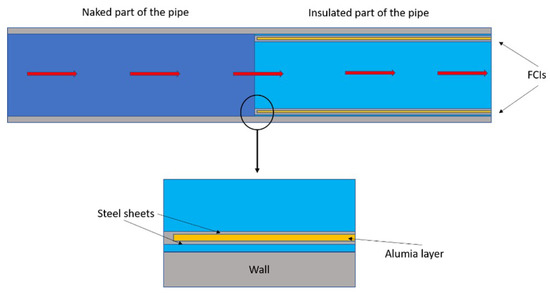
Figure 3.
Sketch illustrating a Flow channel insert example configuration in a pipe (entrance in insulated region). Red arrows define metal liquid path. The FCI “sandwich” structure is highlighted in the bottom.
4. Verification and Validation (V&V)
IAEA guidelines suggest that computer-based tools or calculation methods that could be possibly used in safety analysis must undergo Verification and Validation (V&V) process to assess their reliability and efficiency [20].
The V&V procedure of the RELAP5 MHD module involves the comparison of the results deduced by the code with those of direct numerical simulation tools and data obtained by experimental works. Notable examples of V&V for MHD numerical solvers are found in References [46,47,48,49,50]. At first, simple test cases are employed to verify the response of the program in terms of magnetohydrodynamic pressure drops, either for 2D and 3D phenomena, thus testing the reproduction of a single MHD phenomenon separately. In itself, this is not considered satisfactory to assess the reliability of the code, thus more complex systems are analysed, i.e., two Test Blanket Modules (TBMs) concepts, to demonstrate the capability of the various subroutines of the MHD module to operate together and produce physical results. For this purpose, the numerical analysis performed by Swain et al. in [51] on the Lithium Lead Ceramic Breeder (LLCB) TBM at fusion-relevant magnetic field intensity is repeated with RELAP5 and an excellent quantitative agreement is found on the total pressure drop and local pressure profile.After that, the experimental data produced by the campaign carried out by KIT researchers on a Helium Cooled Lithium Lead (HCLL) TBM mock-up have been considered to further demonstrate the performance of the code against a more realistic benchmark [33]. The module geometry is simulated with the code and, again, an excellent agreement is found in terms of pressure drop prediction. It should be stressed that the HCLL TBM mock-up can be considered by all means a state-of-the-art scaled-down integrated effect test (IET) facility since it represented all relevant isothermal MHD phenomena but for a skewed (toroidal-poloidal) magnetic field that, however, is unlikely to be achieved before the start of the experimental TBM phase in ITER.
4.1. Single Effect Validation
4.1.1. Flow Channel Insert Test Case
The experimental study performed by Bühler et al. in [43] has been employed as test case, to verify the correct behaviour of the code when it comes to treat FCI configurations and fully developed flow pressure drops in circular cross-section conduits.
The reference geometry is a straight pipe (Figure 3 and Figure 4) which is divided in a bare region and in an FCI region (darker in Figure 4). The liquid metal streams from the naked part to the one where the insulation layer is located. Therefore, the LM meets a discontinuity in the wall electrical conductivity that induces an electric potential gradient along the flow direction. For this reason, currents with a three-dimensional path arise in the fluid domain, extra Lorentz forces occur and cause additional loss of load compared with the fully developed flow. This 3D drop must be evaluated properly since, considering it occurs at the exit of FCIs or at gaps between insulation layers, it could significantly reduce the efficacy of flow channel inserts.
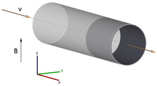
Figure 4.
3D sketch of the experimental section. The darker portion of the pipe is where insulation is applied (FCI). Magnetic field vector B and velocity v are depicted.
The test case is representative of the breeder ingress in the insulated part of the Li-Pb loop since, to minimize complexity and cost, only a small section of it is going to be fitted with inserts.
The molten metal involved in the experiment is a sodium-potassium alloy (NaK, mass fraction: Na 22% K 78%), whereas the horizontal pipe is made of stainless-steel with uniform wall thickness. The flow is treated as isothermal; therefore, materials properties are taken at the reference temperature of 293.15 K (Table 3).
Table 3.
Material properties at 293.15 K.
The magnetic field applied is uniform and unidirectional within the test section domain. Its intensity may be varied, as well as NaK mass flow rate. Thus, the experiment is carried out in a range of nondimensional numbers relevant for fusion reactor applications, that is and ; hence, in the MHD analysis viscous and inertial effects are considered negligible in most of the fluid volume. As crucial results, the experimental campaign observed that the pressure drop (), introduced by the LM entering in an insulated region, corresponds to the pressure loss that would occur in the same insulated pipe about four characteristic lengths (a) long.
In Equation (20), the internal radius of the bare duct is chosen as characteristic length. Factor stands for the nondimensional fully developed flow pressure gradient, defined by Miyazaki et al. in [23]. Moreover, it is worth underlining that Equation (20) seems to be valid in the whole range of the experiment, namely for each Hartmann number and Reynolds number investigated [43]. In Figure 5, the meshing scheme employed for calculations is shown. Inlet conditions of the liquid metal are imposed by a time-dependent volume (TMDPVOL ) and a time-dependent junction (TMDPJUN ). The TMDPVOL sets NaK inlet temperature and the TMDPJUN imposes the liquid metal mass flow rate. The liquid outlet pressure is fixed by an additional time-dependent volume (TMDPVOL ). A pipe component (PIPE ) is used to model the conduit, that is divided in 15 single volumes, thus, linked by 14 single junctions. In the last 10 volumes, the isolation layer is applied; this is accomplished by modelling thinner stainless-steel walls, in order to obtain the same conductance ratio that is reported by Bühler, [43]. In Table 4, the main parameters are reported.
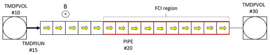
Figure 5.
Sketch of the model, outlining RELAP5 discretization. The region where flow channel insert is applied is underlined in red. With yellow arrows is delineated the fluid path.
Table 4.
Model geometry parameters.
The trend of the scaled pressure versus the nondimensional axial length (x) is shown in Figure 6. The pressure is scaled with reference value Pa, whereas all geometrical parameters are scaled through characteristic length a.
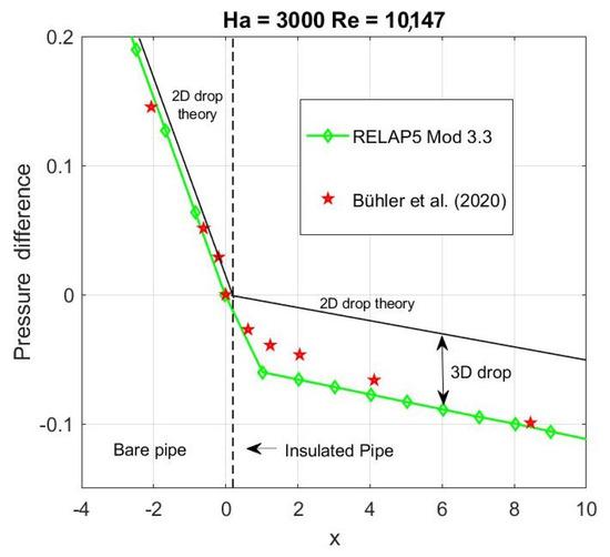
Figure 6.
Total nondimensional pressure drop versus scaled axial length. Vertical dashed line states the beginning of the insulated part of the conduit. The deviation, between fully developed flow theory and numerical/experimental outcomes, that exists after is due to three-dimensional pressure drop.
Is important to underline that the general behaviour of the nondimensional pressure loss found by Bühler is very similar for every and values; for this reason, results for other governing parameters are not reported. In the whole pipe, it can be observed the very good agreement that RELAP5 has with both theoretically predicted pressure loss and experimental results. The nondimensional pressure gradient computed by the code completely matches the one reported by Miyazaki for circular conduits (black line in Figure 6).
In Table 5, are gathered numerical results for several calculations performed. The code shows an excellent accuracy (relative errors ) in evaluating fully developed flow loss of load and the absolute value of three-dimensional pressure drop is detected with good precision (discrepancy ). The slight over-valuation regarding localized losses can be explained as follows: beside a discontinuity in wall electrical conductance, the flow also faces a moderate cross-section contraction due to the presence of insulation structure. Hence total 3D head loss, expressed by Equation (20), comprehends the contribution of a sudden cross-section contraction that, however, is challenging to extrapolate. Therefore, considering that the RELAP5 FCI model is based on experimental outcomes that usually include these contraction/expansion contributions, the discrepancy of with the experimental data in the present test case is because of the cross-section variation being taken into account twice by RELAP5: with the activation of the flow channel insert model and the cross-section restriction model.
Table 5.
Relative errors of numerical results compared with theory/experimental outcomes.
4.1.2. Sudden Cross-Section Variations
The experimental analysis carried out by Buhler and Horanyi in [32] is used as a benchmark for verifying RELAP5 model for 3D MHD pressure drop due to a sudden change of the duct cross-section. Furthermore, it is also useful to demonstrate the capability of the code to predict 2D pressure loss occurring in square/rectangular conduits. The experiment characterizes a liquid metal (NaK) flow within a rectangular duct that undergoes a sudden cross-section expansion, after which the conduit cross-section is a square (Figure 7). The duct expands only along the magnetic field direction; therefore, the cross-section variation is purely parallel. The expansion ratio is defined as Z = 4 and the conductance ratio of the expanded channel is (see Table 6 for geometrical details). When the fluid approaches the variation, it undergoes a velocity redistribution to rearrange its structure that induces an axial potential difference. Consequently, stream-wise electrical currents arise and, interacting with the strong magnetic field, they generate extra Lorentz forces that are responsible for the additional pressure drop (). The test section is made of stainless-steel with uniform wall thickness, both upstream and downstream of the expansion. The flow is horizontal and isothermal, so that thermo-physical properties of the materials are evaluated at the constant temperature of 293.15 K (see Table 3). The magnetic field, considered uniform and unidirectional, is applied along the expansion direction. The experiment is conducted in a range of nondimensional numbers and [32].
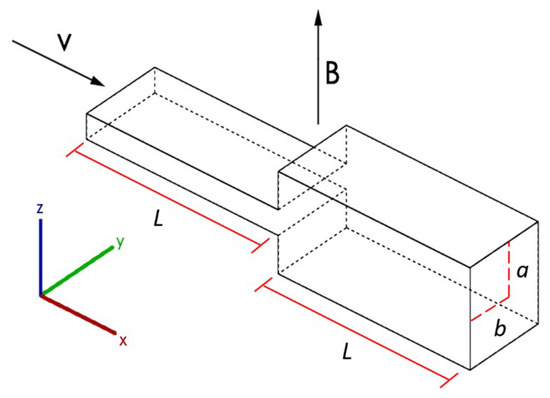
Figure 7.
Geometry sketch of the experimental section.
Table 6.
Model geometry parameters.
In Figure 8, is shown the nodalization scheme of the model. Fluid inlet conditions are established by a time-dependent volume component (TMDPVOL ) and a time-dependent junction (TMDPJUN ). The TMDPVOL provides metal inlet temperature and the TMDPJUN sets the mass flow rate. The liquid outlet pressure is fixed by another time-dependent volume (TMDPVOL ). A pipe component (PIPE ) simulates the duct, that is divided in 12 single volumes linked by 11 single junctions. In Table 6, the main parameters of the model are reported.
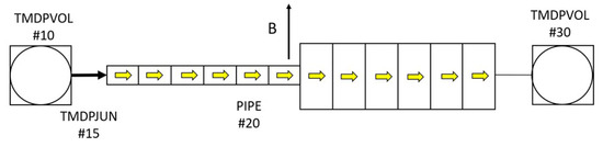
Figure 8.
Sketch of the RELAP5 nodalization. Yellow arrows mark the fluid path. Magnetic field (B) is shown with a black vector.
In Figure 9, is shown a representative trend of the scaled pressure versus the nondimensional axial length. The pressure is scaled with and all geometrical parameters through the characteristic length a = 0.047 m. In the region where the flow is fully developed, according to Bühler, the nondimensional pressure gradient is for the rectangular pipe, whereas in the square one, for the governing parameters and 29,604.
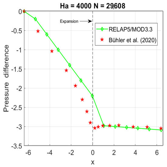
Figure 9.
Total nondimensional pressure drop versus scaled axial length for and . Vertical dashed line points the sudden expansion.
As reported in Table 7, RELAP5 detects with great accuracy the pressure gradient due to MHD 2D phenomena in square/rectangular conduits, with a relative error always lower than . Furthermore, also the total 3D loss is well predicted by the code, that provides accurate results if compared with the ones of Equation (19).
Table 7.
2D and 3D pressure losses errors, for different and N.
4.2. Multiple Effect Validation
4.2.1. Lithium Lead Ceramic Breeder TBM
Computational fluid-dynamic analysis of MHD flow in a full-scale variant of the proposed Lithium–Lead cooled Ceramic Breeder Test Blanket Module proposed by India for the ITER experimental campaign, has been performed, at fusion-relevant Hartmann number (), by Swain et al. in [51].
Numerical MHD studies at high magnetic field for such complex configurations are rare and they provide precious results for the system codes verification phase. In [51], an exhaustive thermal-hydraulic analysis is performed; for the aim of this work, however, the attention is focused on the pressure drop outcomes.
In Figure 10a, a two-dimensional sketch that describes the TBM geometry and flow path is represented. The LM involved is Li-Pb and enters the module through an inlet header channel (segment A-B). After that, the fluid is driven upward through five vertical (poloidal) channels (segment B-C). The poloidal channels are numbered from 1 to 5 moving away from the return channel, with Channel 1 being the closest to the latter. Consequently, the fluid is collected in top header region and then it goes down in the poloidal return channel (segment D-E). At last, the lithium-lead gathers in the outlet header (E-F) before leaving the TBM. All Li-Pb ducts have rectangular cross-section. The LM is the coolant used to extract thermal power from the breeding zone, which is constituted by boxes filled with the solid breeder (lithium-titanate) and enclosed by thin Reduced-Activation Ferritic-Martensitic steel (RAFMS) walls. For the purpose of MHD calculations, the breeder modules can be assumed as perfectly insulating and only the bounding walls must be considered to estimate the equivalent wall conductivity. Geometrical parameters are consistent with those reported in [51], and are collected in Table 8. Thermo-physical properties of RAFMS and Li-Pb are evaluated at the reference temperature of 623 K and the flow is assumed to be purely isothermal. Magnetic field B is set at 4 T and assumed to be unidirectional and aligned with the toroidal axis. Mass flow rate imposed at the inlet is equal to 12 kg/s.
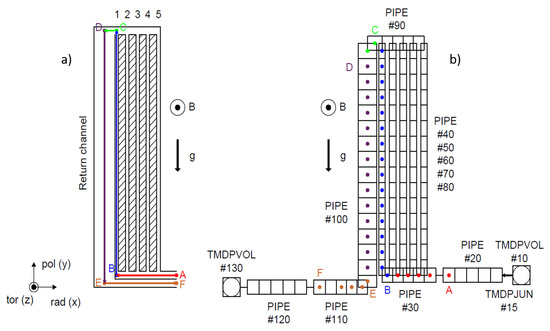
Figure 10.
(a) 2D scheme of the LLCB TBM. Shaded area represents the breeding modules. (b) Nodalization of the geometry.
Table 8.
Main geometrical parameters of LLCB flow path [51].
The nodalization scheme, developed on the geometry presented in Figure 10a, is reported in Figure 10b. It is composed of 118 control volumes and 121 hydraulic junctions. The sliced modelling approach is applied, assuming the same length for the vertically oriented volumes at the same level. Inlet conditions of the liquid metal are imposed by a time-dependent volume (TMDPVOL # 10) and a time-dependent junction (TMDPJUN # 15). The TMDPVOL sets Li-Pb inlet temperature and the TMDPJUN imposes the liquid metal mass flow rate. The Li-Pb outlet pressure is fixed by an additional time-dependent volume (TMDPVOL # 130). All the sections composing the TBM have been modelled with equivalent pipe components. The modelling approach is to keep actual inventory and flow area for each section. Hydraulic k-loss coefficients for abrupt area changes, bends and tees have been evaluated using the correlations presented in Idel’chik handbook [52] and are used to obtain a reliable figure for the ordinary hydrodynamics. The coloured markers in Figure 10b (refer to the online version of the paper) identify the acquisition points of the pressure within the model. The same colours are associated with the characteristic hydraulic elements reported in Figure 10a: red (inlet header), blue (poloidal channel), green (top header), purple (return channel), orange (outlet header). The differential pressure for the i-th control volume is evaluated as follows: , where is the pressure acquired in the i-th control volume, is the pressure acquired in the F position, is the Li-Pb density, g is the gravitational acceleration and is the elevation difference between the i-th control volume and the F level.
Before the main numerical campaign, a purely hydrodynamic simulation, imposing B = 0 T, is performed in [51] to quantify the weight of magnetohydrodynamic effects over inertial and viscous ones. The same simulation is repeated with RELAP5 to assess the efficacy of the geometrical and nodalization model chosen. Excellent results, in terms of mass flow rate distribution in vertical channels, are obtained with the code; the discrepancy from the numerical analysis is lower than 3.7% in each channel. In Table 9, the comparison is summarized. As a reference, the pressure loss in the hydrodynamic LLCB TBM is estimated at 0.432 kPa, approximately 1.2% of the pressure loss estimated by the MHD model.
Table 9.
Mass flow rate outcomes for ordinary hydro-dynamic case (), comparison between CFD analysis and RELAP5. (*) Inlet total mass flow rate as boundary condition.
Once the input geometry is proven efficient, the calculation with is carried out. Reference governing parameters are = 17,845 and ; the characteristic length is the toroidal half-length of the whole module, namely a = 0.214 m. In Figure 11, it is reported the dimensional pressure drop versus axial length, occurring in the fluid path that is underlined with coloured segments in Figure 10a. It can be noticed that RELAP5 accurately predicts the total pressure drop, with a relative error that is . It is worth reminding that magnetic field is always directed perpendicular to the blanket module. Therefore, this calculation demonstrates that the 3D MHD models implemented for bends and cross-section variations occurring perpendicular to B are reliable to simulate even a complex geometry like the one considered in this study.
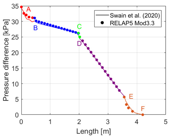
Figure 11.
Pressure drop trend along the specified fluid path, for = 17,845 and .
Nevertheless, it is important to point out a significant shortcoming of our code. As mentioned, RELAP5 is not currently capable of recreating electromagnetic coupling effects, like the ones that exist in the LLCB due to the sharing of an electrically conductive wall between Channel-1 and the return channel. The lack of this feature is made quite noticeable by the huge difference that is found between the RELAP5 and CFD predictions of the mass flow rate distribution across the TBM vertical channels, as it is shown in Table 10.
Table 10.
Mass flow rate outcomes for MHD (), comparison between CFD analysis and RELAP5.
According to Swain’s CFD calculation, the presence of electromagnetic coupling phenomena accentuates the imbalance of mass flow rate in poloidal channels, that in the OHD case is due to inertial forces only. As a matter of fact, the numerical pressure gradient of Channel-1 is significantly decreased by local electrical coupling effects due to its adjacency with the counter-flowing return channel that, assuming uniform flow distribution, carries as much as five times its flow rate. A qualitative explanation, cfr. Figure 12, can be given as follow. Due to the electrical contact between the two channels, currents generated in one can leak and close through the other. Since , the currents induced in the return channel are stronger in magnitude than those in Channel-1, due to the larger flow rate there. When these currents close through Channel-1, they promote the fluid movement rather than opposing it, as they would have in their original conduit, since . Velocity increases in Channel-1 until the resistive Lorentz force generated by currents induced in is enough to compensate the leakage currents.
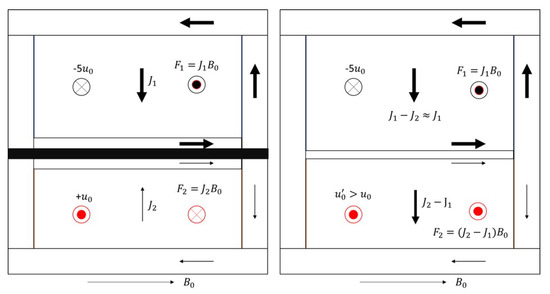
Figure 12.
(Left) If the return (top) and Channel-1 (bottom) are not in electrical contact, i.e., separated by a thin layer of perfect electrical insulation (black band), no leakage currents can be exchanged and, in general, due to the different flow rate. Lorentz force self-induced in the two channels opposes the flow movement. (Right) if the channels are in electrical contact, currents from the return channel can close through Channel-1 and induce a net promoting Lorentz force that increases the flow rate in it. The increase in average velocity eventually makes and the balance is restored with the reappearance of a retarding Lorentz force in Channel-1.
The macroscopic effect is that Channel-1 draws more flow rate than the other poloidal channels, from which the flow imbalance observed by Swain et al. in [51]. Furthermore, counter-flow coupling effects influence also the flow in the inlet and outlet header where a substantial flow rate difference exists, in particular, in the region close to Channel-1 and Channel-2. This behaviour further favours a net decrease of the resistance offered by the route through Channel-1 (and, to a lesser degree, Channel-2). It is worth noticing that, instead, electro-coupling does not radically affect poloidal channels 3–5, since they are divided by solid breeder modules.
Aforementioned phenomena cannot be modelled by RELAP5 that, therefore, is going to compute the flow distribution across the poloidal channels exclusively according to the 2D and 3D pressure losses occurring therein. Inertial effects are almost negligible at and and, consequently, the result is an almost uniform flow distribution. Differently put, the main source of mass flow rate disequilibrium in hydro-dynamic calculation (inertia), is completely overcome by magnetohydrodynamic effects that, anyhow, are significantly affected by electromagnetic coupling in this specific configuration. It can be concluded that in its current state RELAP5 MHD module is not suitable to estimate the flow rate distribution in a manifold featuring one or more channels in electrical contact with an adjacent-counter-flowing duct with a very large flow rate. Nevertheless, it should be highlighted that the feature that the code is currently lacking, seems to not affect the pressure drop calculation in this configuration significantly, as can be observed by the results reported in Table 11, which surprisingly match quite well the prediction from the CFD code. A possible explanation of this unintuitive behaviour is provided in the following.
Table 11.
Pressure drop differences in counterflow electro-coupled conduits (B = 4 T).
The major part of the overall pressure drops of the TBM, more than 50%, takes place in the return channel as is shown in Table 11. This happens because in the return channel the velocity is larger than the one in the poloidal ascending conduits and the expansions/contractions contributions are more important. Conversely, the effect of electrical coupling within the descending channel is weak (negligible), as it is also highlighted by the results of Swain et al. (Table 4 in [51]), where the numerical pressure gradient is observed to be very close to the theoretical one (which, of course, neglects coupling). Consequently, RELAP5 is able to compute consistently the “leading” pressure drop source within the whole TBM. Moreover, it is important to keep in mind that electrocoupling primary decreases distributed pressure losses (2D MHD), which are linearly dependent by the the fluid mean velocity. On the other hand concentrated drops (3D MHD), that are also linear with velocity, are not significantly affected by the coupling. The good agreement in terms of total pressure drop in the poloidal Channel-1 between RELAP5 and CFD computation (see Table 11), despite a substantial mass flow rate difference, could be due to an overall compensation of 2D and 3D MHD losses (referring to the relations expressed in Equations (1) and (2)). In [51], 2D MHD drops are reduced by coupling, whereas 3D MHD ones are increased due to the high mean velocity in the conduit; RELAP5 numerical model instead provides higher MHD distributed losses since the coupling is not taken in account but the local MHD drops are less influential considering the moderate average fluid velocity. However, it is crucial to underline that this discussion is strictly valid only for the specific geometrical configuration of the LLCB TBM, since electrocoupling phenomena deeply depend on multi-channel arrangement.
To summarize, the MHD module of RELAP5 has demonstrated the capacity to provide results which are consistent with the prediction from a direct numerical simulation code in terms of electromagnetic pressure loss. A lack of fidelity is highlighted in the estimate of mass flow distribution for a manifold feeding channels which are in electrical contact with adjacent counter-flowing ducts with large flow rates. This is caused by the absence of a dedicated electromagnetic coupling model.
4.2.2. Helium Cooled Lithium Lead TBM Mock-Up
MHD flow in a scaled mock-up of a Helium Cooled Lithium Lead test blanket module for ITER has been experimentally investigated by Bühler et al. in [33] to gather experimental data to support the proposed design concept and as a benchmark for validation of numerical tools. As one of the few experimental campaigns involving a geometry representative of the complexity of a fusion reactor blanket design, this benchmark is considered the most suitable to demonstrate the validity of the numerical approach adopted by RELAP5. The HCLL mock-up is scaled down by a factor of 2 compared with the TBM to fit into the experimental facility MEKKA. Experimental data have been collected in a wide range of parameters: and .
The fluid adopted for the experiment is NaK, whereas the structural material is stainless steel. Thermo-physical properties of involved materials are taken at the operating temperature of 293 K (see Table 3). The HCLL geometry is very complicated and the fluid undergoes numerous bends and sudden cross-section variations. A two-dimensional scheme of the flow path is depicted in Figure 13. The mock-up encompasses two parallel breeding units (BUs), each one being composed by an inflow unit (D-E) and an outflow unit (F-G). Liquid metal enters the TBM at position A, which corresponds to the beginning of the feeding pipe (with circular cross section). After, it is collected in the inlet manifold, that serves to distribute the flow rate in the two breeding units. The manifold is composed by a tall and narrow rectangular duct realized between the BU back plate and the mock-up external plate (Figure 14). The connection with the feeding pipe is realized in a larger cavity that undergoes a sudden contraction of about 50% in the magnetic field direction at the height of the first dashed line in Figure 13. The narrower conduit conveys the fluid to the second BU and it is gradually tapered to 50% of its original cross-section until the third dashed line in Figure 13. The geometry of the outlet manifold mirrors the previous one: gradually increasing cross-section, sudden expansion and connection with the draining pipe. It should be noted that helium manifolds, that will reduce the available cross-section for the LM in its manifold, were not included in the mock-up and they are, similarly, not included in RELAP5 [33]. The interface between manifold and BUs is ensured through an elongated narrow orifice in the BU back plate. Once inside the inflow unit, the fluid is subjected to another subdivision due to the presence of thin metal plates that partitions the volume in 6 parallel channels, simulating the presence of helium cooling plates. At the first wall (FW), the liquid meets an elongated and narrow toroidal-radial orifice that allows hydraulic connection with the outflow unit. The LM is then gathered in the outlet manifold and leaves the TBM through the draining pipe [33]. In Table 12, are gathered the dimensions of the mock-up.
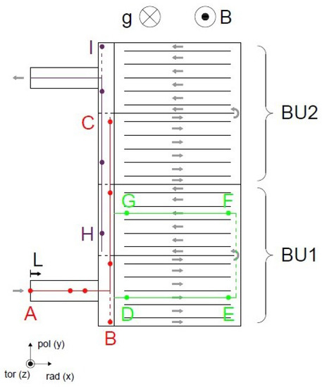
Figure 13.
2D view (radial-poloidal) of the TBM geometry. The flow path underlined with colored segments (A-I) is used in the following for pressure drop calculation.
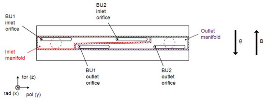
Figure 14.
Toroidal-poloidal view of the mock-up. In red is outlined the feeding manifold, whereas in purple the collecting one. Cross-section shape of both inlet/outlet pipes and manifold/BU interface are reported.
Table 12.
Main geometrical parameters. (*) Average toroidal length of the narrow manifold along poloidal direction. (**) Cooling plates dimensions are not reported [33].
The nodalization scheme adopted is reported in Figure 15. Two time-dependent volumes define the inlet temperature and the outlet pressure of the NaK alloy. The liquid metal mass flow rate is imposed by the time-dependent junction, connecting the inlet TMDPVOL and the inlet conduit (PIPE #20 in Figure 15). Inlet and outlet manifolds are simulated with two equivalent pipes. Each one is composed of three control volumes (CVs), reproducing the relevant configuration of the component. Focusing on the inlet manifold, the first and the third CVs simulate the inlet chambers, adjacent to the first interface between manifold and breeding units. The second CV reproduces the connection between those. For the first and the third control volumes, the flow along the radial direction is selected. This approach allows to estimate the actual abrupt area change in the interface with the breeding zone (BZ). The two BUs are simulated with two pipe components. The six channels composing the BU are collapsed in an equivalent single pipe, characterized by total flow area, equivalent hydraulic diameter and geometrical parameters relevant for MHD analysis of a single representative channel, namely one of the four at the centre of the cell. Each pipe component consists of seven CVs, reproducing inlet and outlet holes, the radial channels and the inversion chamber. Coloured markers, in both Figure 13 and Figure 15, mark the position of pressure acquisition data points within the mock-up and RELAP5 numerical model.
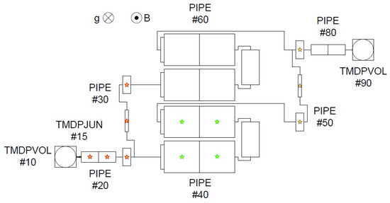
Figure 15.
Meshing scheme of the geometry.
Figure 16 shows the comparison between experimental and RELAP5 data for nondimensional pressure drop along the flow path A-I (i.e., coloured lines in Figure 13) with respect to the pressure measured in point A. the characteristic length chosen is the toroidal half-length of BU, namely a = 0.045 m, whereas pressure is scaled with Pa. As for cases previously studied, the pressure scaling employed allows, for a single Hartman number investigated, to condense the results for various Reynolds numbers in a unique representation. Furthermore, it confirms that MHD flows at fusion conditions are not affected by relevant inertia phenomena. For this reason, only few results are reported in graphical form.
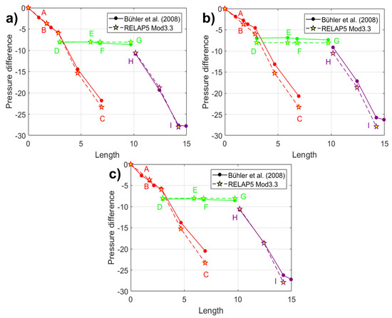
Figure 16.
Nondimensional pressure drop versus scaled length. Comparison of results between R5 and reference experiment. (a) . (b) . (c) .
As can be observed, pressure drop mostly occurs in the circular inlet conduit (A–B) and in the inlet/outlet manifolds (B–C and H–I), since the velocities here are much higher than in BUs due to the smaller cross sections. Moreover, the walls of pipes and manifolds are thicker, hence their wall conductance ratios generally increased compared with the ones in breeder units (). Those features provide higher currents and, therefore, more intense Lorentz forces causing greater pressure head losses. Furthermore, additional contributions to pressure loss occur because the fluid is forced to pass through narrow orifices into and out of the breeder units (B–D and G–H). Here, three-dimensional MHD effects arise and induce an additional pressure drop. The contraction (and the following expansion) of the fluid into the narrow gap between inflow/outflow units (dashed line E–F) and the bend at the first wall, have no substantial effect on the loss of load, since they occur in a plane perpendicular to B. It is noticed that the pressure loss in the breeding cells (D–E and F–G) where the fluid has a moderate velocity (≈1 mm/s) is negligible, especially when compared with the one occurring in pipes/manifolds.
RELAP5 shows an excellent agreement with experimental results. In Table 13, as example, outcomes and relative errors for two the calculations performed at are reported. In general, is observed an excellent prediction of the total pressure loss, with a discrepancy that is . This is a crucial result, since it clearly demonstrates that RELAP5 is suitable to predict pressure losses even in relatively complex geometries as the one proposed for the HCLL TBM.
Table 13.
Pressure drop results (nondimensional) for every position of flow path and total loss. Relative Errors are reported.
As discussed for LLCB, the main drawback of the code in the current version is the lack of modelling for electromagnetic coupling, which is the main source of error of RELAP5 calculation. In [33], electrical coupling effects are demonstrated to be influential in the flow rate distribution, in particular among internal channels of BUs. Nevertheless, the pressure drop is significantly reduced in the breeding unit, thus the lack of a coupling model in the code does not essentially influence the prediction of pressure loss. It should also be noted that the code slightly over-predicts the pressure loss due to the cross-section variations; this is particularly evident in the connection between manifold and breeding unit (B–D and G–H). This is a consequence of the conservative assumptions adopted for the development of the 3D pressure loss model for this component; the estimate is likely to improve once more data will be available to fine tune it. As a final note, it is worth mentioning that the lower accuracy that the code shows for results at could be attributed to an anomaly related to experimental data acquisition, considering that RELAP5 performance is substantially the same for and .
5. Conclusions and Further Works
A new module for the best-estimate SYS-TH code RELAP5/MOD3.3 has been developed at Sapienza, University of Rome, allowing the program to model MHD pressure drop in liquid metal circuits. Two-dimensional and three-dimensional MHD pressure losses, akin to distributed and concentrated friction losses in ordinary hydrodynamic flow, are modelled for a wide range of geometries. These features are of particular interest for fusion related activities and, in particular, for the design of liquid breeding blankets, where MHD pressure loss is the dominant component. In its current state, the code is deemed suitable for the simulation of liquid metal breeding blankets and circulating loops in normal operation and postulated transients that do not involve a rapid time variation of the reactor magnetic field. Application of the code to the prediction of non-isothermal transients for these systems must be carefully considered since MHD effects on heat transfer have not yet been implemented.
A Verification and Validation (V&V) campaign is performed, using several numerical and experimental studies as benchmark, to demonstrate the capacity of the code of reproducing physical results. In a first step, sub-routines are validated independently (single effect) to ensure their correct operation. Subsequently, RELAP5 is used to recreate the results obtained by direct numerical simulation tools and experimental campaigns in two Test Blanket Modules, i.e., the LLCB [51] and HCLL [33]. It is found that MHD subroutines of RELAP5/MOD3.3 are reliable in modelling electromagnetic effects that are crucial in the pressure drop assessment of fusion related LM circuits. Two-dimensional loss is well predicted by the code, with a discrepancy with respect to the numerical/experimental outcomes that is always around 1%. This certainly makes the code competitive, in terms of capability, with other numerical tools that can handle this level of analysis, such as MARS-FR [13] and MHD-SYS [17] (Section 1). Furthermore, RELAP5 three-dimensional MHD pressure drop module assures good agreement with TBM validation test cases results, with a discrepancy that is generally ; this is mostly due to the conservative approach that has been employed to develop 3D pressure drop models, needed to overcome the physical uncertainties that still exist in the prediction of those phenomena. Albeit the code is lacking a dedicated subroutine to represent electro-coupling phenomena, the absence of such a model does not affect significantly the pressure drop analysis, but rather the capacity of the code in predicting mass flow rate distribution when multichannel configurations occur. It should be remarked that the excellent agreement with the HCLL TBM experimental data is a result that demonstrates the code scalability to reactor conditions since the HCLL mock-up can be considered by all means a IET facility. In conclusion, the code development discussed in this paper has significantly increased the capability of the modified RELAP5, that now can be considered a reliable tool for magnetohydrodynamic pressure drop evaluations in liquid metal circuits.
The current version of the code is still far from an ideal implementation since several important features, such as an electromagnetic coupling model, are still lacking and correlations for 3D MHD losses must be refined to extend their flexibility and range of validity. It should be stressed that these limitations reflect a lack of theoretical understanding for the former case and inconsistent experimental data for the latter and, thus, are likely to be improved as the knowledge progresses. Future activities will be focused on the expansion of bend and cross-section variation modelling for arbitrary wall conductivity. Preliminary work has already been done for the definition of an electromagnetic coupling model based on the analytical solution presented by Bluck et al. [53]. Implementation of other relevant configurations that imply localized loss of load, such as fringing magnetic field or MHD flow around obstacles, is currently being considered, as well as to extend the support to the modelling of perfectly insulated walls. To complete the picture of MHD phenomena in the breeding blanket of a fusion reactor, the next phase of development will be dedicated to implement a MHD heat transfer models. It is planned to derive, at first, a basic model for MHD forced convection heat exchange mechanism that, afterwards, could be extended to include buoyancy effects (mixed convection). Subsequently, a model for evaluating MHD influence on tritium transport is foreseen to be developed if the research about this topic will be intensified, as proposed by Seo et al. in [10]. At last, whenever MHD phenomena caused by a strong time-varying magnetic field will be better characterize in the literature, the models are foreseen to be updated so that a wider range of scenarios (operational or incidental) could be possibly simulated by the code.
Author Contributions
Conceptualization, A.T., L.M., F.G. and G.C.; methodology, A.T., L.M.; software, L.M. and V.N.; validation, V.N., L.M. and A.T.; formal analysis, V.N., L.M. and A.T.; investigation, L.M., A.T. and V.N.; writing—original draft preparation, L.M.; writing—review and editing, A.T., L.M., V.N. and G.C.; visualization, L.M. and V.N.; supervision, A.T.; project administration, A.T. and G.C.; funding acquisition, F.G., G.C. All authors have read and agreed to the published version of the manuscript.
Funding
This work has been carried out within the framework of the EUROfusion Consortium and has received funding from the Euratom research and training program 2014–2018 and 2019–2020 under grant agreement No 633053. The views and opinions expressed herein do not necessarily reflect those of the European Commission.
Institutional Review Board Statement
Not applicable.
Informed Consent Statement
Not applicable.
Data Availability Statement
Not applicable.
Acknowledgments
The authors wish to thank Joelle Vallory and Italo Ricapito, for their preliminary review of the paper and effective suggestions. A heartfelt thanks to Elisa Martino, for her precious help with several images reported in this paper.
Conflicts of Interest
The authors declare no conflict of interest.
Abbreviations
The following abbreviations are used in this manuscript:
| BB | Breeding Blanket |
| BE | Best Estimate |
| BU | Breeding Unit |
| BZ | Breeding Zone |
| CFD | Computational Fluid-Dynamic |
| DIAEE | Dipartimento di Ingegneria Astronautica, Elettrica ed Energetica |
| ENEA | Agenzia Nazionale Energie Alternative |
| EU-DEMO | EUropean DEMOnstration Power Plant |
| FCI | Flow Channel Insert |
| FW | First Wall |
| HCLL | Helium-Cooled Lithium–Lead |
| ITER | International Thermonuclear Experimental Reactor |
| KIT | Karlsruher Institut für Technologie |
| LLCB | Lithium–Lead Ceramic-Breeder |
| LM | Liquid Metal |
| MEKKA | Magneto-hydrodynamische Experimente in Natrium Kalium Karlsruhe |
| MHD | MagnetoHydroDynamic |
| OHD | OrdinaryHydroDynamic |
| RAFMS | Reduced-activation Ferritic/Martensitic Steel |
| RELAP5 | Reactor Excursion Leak Analysis Program |
| SYS-TH | SYStem Thermal-Hydraulic |
| TBM | Test Blanket Module |
| TMDPJUN | TiMe-DePendent JUNction |
| TMDPVOL | TiMe-DePendent VOLume |
| V&V | Verification and Validation |
| WCLL | Water-Cooled Lithium–Lead |
References
- EUROfusion. European Research Roadmap to the Realisation of Fusion Energy; EUROfusion Programme Management Unit: Garching/Munich, Germany, 2018. [Google Scholar]
- Smolentsev, S. Physical background, computations and practical issues of the magnetohydrodynamic pressure drop in a fusion liquid metal blanket. Fluids 2021, 6, 110. [Google Scholar] [CrossRef]
- Smolentsev, S.; Spagnuolo, G.A.; Serikov, A.; Rasmussen, J.J.; Nielsen, A.H.; Naulin, V.; Marian, J.; Coleman, M.; Malerba, L. On the role of integrated computer modelling in fusion technology. Fusion Eng. Des. 2020, 157, 111671. [Google Scholar] [CrossRef] [Green Version]
- Smolentsev, S.; Moreau, R.; Bühler, L.; Mistrangelo, C. MHD thermofluid issues of liquid-metal blankets: Phenomena and advances. Fusion Eng. Des. 2010, 85, 1196–1205. [Google Scholar] [CrossRef]
- Tassone, A.; Caruso, G.; Del Nevo, A. Influence of PbLi hydraulic path and integration layout on MHD pressure losses. Fusion Eng. Des. 2020, 155, 111517. [Google Scholar] [CrossRef]
- Kirillov, I.R.; Reed, C.B.; Barleon, L.; Miyazaki, K. Present understanding of MHD and heat transfer phenomena for liquid metal blankets. Fusion Eng. Des. 1995, 27, 553–569. [Google Scholar] [CrossRef] [Green Version]
- Tassone, A.; Siriano, S.; Caruso, G.; Utili, M.; Del Nevo, A. MHD pressure drop estimate for the WCLL in-magnet PbLi loop. Fusion Eng. Des. 2020, 160, 111830. [Google Scholar] [CrossRef]
- Reimann, J.; Benamati, G.; Moreau, R. Report of Working Group MHD for the Blanket Concept Selection Exercise (BSE); Forschungszentrum Karlsruhe GmbH: Karlsruhe, Germany, 1995. [Google Scholar]
- Smolentsev, S.; Badia, S.; Bhattacharyay, R.; Bühler, L.; Chen, L.; Huang, Q.; Jin, H.G.; Krasnov, D.; Lee, D.W.; De Les Valls, E.M.; et al. An approach to verification and validation of MHD codes for fusion applications. Fusion Eng. Des. 2015, 100, 65–72. [Google Scholar] [CrossRef] [Green Version]
- Seo, S.B.; Hernandez, R.; Neal, M.O.; Meehan, N.; Novais, F.S.; Rizk, M.; Maldonado, G.I.; Brown, N.R. A review of thermal hydraulics systems analysis for breeding blanket design and future needs for fusion engineering demonstration facility design and licensing Figure of Merit. Fusion Eng. Des. 2021, 172, 112769. [Google Scholar] [CrossRef]
- Bestion, D. The Structure of System Thermal-Hydraulic (SYS-TH) Code for Nuclear Energy Applications; Elsevier Ltd.: Amsterdam, The Netherlands, 2017; pp. 639–727. [Google Scholar] [CrossRef]
- Code Development Team. RELAP5-3D Code Manual: Code Structure, System Models and Solution Methods.; Idaho National Laboratory (INL): Idaho Falls, ID, USA, 2015; Volume I.
- Kim, S.H.; Kim, M.H.; Lee, D.W.; Choi, C. Code validation and development for MHD analysis of liquid metal flow in Korean TBM. Fusion Eng. Des. 2012, 87, 951–955. [Google Scholar] [CrossRef]
- Panayotov, D.; Grief, A.; Merrill, B.J.; Humrickhouse, P.; Trow, M.; Dillistone, M.; Murgatroyd, J.T.; Owen, S.; Poitevin, Y.; Peers, K.; et al. Methodology for accident analyses of fusion breeder blankets and its application to helium-cooled pebble bed blanket. Fusion Eng. Des. 2016, 109–111, 1574–1580. [Google Scholar] [CrossRef]
- Grief, A.; Owen, S.; Murgatroyd, J.; Panayotov, D.; Merrill, B.; Humrickhouse, P.; Saunders, C. Qualification of MELCOR and RELAP5 models for EU HCLL TBS accident analyses. Fusion Eng. Des. 2017, 124, 1165–1170. [Google Scholar] [CrossRef]
- Panayotov, D.; Grief, A.; Merrill, B.J.; Humrickhouse, P.W.; Murgatroyd, J.T.; Owen, S.; Saunders, C. Uncertainties identification and initial evaluation in the accident analyses of fusion breeder blankets. Fusion Eng. Des. 2018, 136, 993–999. [Google Scholar] [CrossRef]
- Wolfendale, M.J.; Bluck, M.J. A coupled systems code-CFD MHD solver for fusion blanket design. Fusion Eng. Des. 2015, 98-99, 1902–1906. [Google Scholar] [CrossRef]
- Froio, A.; Batti, A.; Nevo, A.D.; Savoldi, L.; Spagnuolo, G.A.; Zanino, R.; Energia, D.; Torino, P.; Kessel, C.; Staack, G.; et al. Implementation of a System-Level Magnetohydrodynamic Model in the GETTHEM Code for the Analysis of the EU DEMO WCLL Breeding Blanket. In Proceedings of the Technology Of Fusion Energy (TOFE) Conference, Charleston, SC, USA, 20–23 April 2020. [Google Scholar]
- Batti, A. System-Level Hydraulic Modeling of the PbLi Loop for the Breeding Blanket of a Tokamak; Politecnico di Torino: Turin, Italy, 2020. [Google Scholar]
- International Atomic Energy Agency (IAEA). Safety Assessment for Facilities and Activities; Technical Report; IAEA: Vienna, Austria, 2016. [Google Scholar]
- Müller, U.; Bühler, L. Magnetofluiddynamics in Channels and Containers; Springer: Berlin, Germany, 2001. [Google Scholar] [CrossRef]
- Madarame, H.; Taghavi, K.; Tillack, M.S. Influence of Leakage Currents on Mhd Pressure Drop. Fusion Technol. 1985, 8, 264–269. [Google Scholar] [CrossRef]
- Miyazaki, K.; Kotake, S.; Yamaoka, N.; Inoue, S.; Fujiie, Y. MHD pressure drop of NaK flow in stainless steel pipe. Nucl. Technol. 1983, 4, 447–452. [Google Scholar] [CrossRef]
- Miyazaki, K.; Inoue, S.; Yamaoka, N.; Horiba, T.; Yokomizo, K. Magneto-Hydro-Dynamic Pressure Drop of Lithium Flow in Rectangular Ducts. Fusion Technol. 1986, 10, 830–836. [Google Scholar] [CrossRef]
- Nuclear Safety Analysis Division. RELAP5/MOD3.3 Code Manual Volume I: Code Structure, System Models and Solution Methods; Idaho National Laboratory: Idaho Falls, ID, USA, 2003; Volume I.
- Giannetti, F.; D’Alessandro, T.; Ciurluini, C. Development of a RELAP5 Mod3.3 Version for FUSION Applications; Sapienza DIAEE internal report D1902_ENBR_T01; Sapienza University of Rome: Rome, Italy, 2019. [Google Scholar]
- Narcisi, V.; Melchiorri, L.; Giannetti, F.; Caruso, G. Assessment of relap5-3d for application on in-pool passive power removal systems. In Proceedings of the 30th European Safety and Reliability Conference and the 15th Probabilistic Safety Assessment and Management Conference, Venice, Italy, 1–5 November 2020; Research Publishing: Singapore, 2020; pp. 1135–1142. [Google Scholar] [CrossRef]
- Narcisi, V.; Melchiorri, L.; Giannetti, F. Improvements of RELAP5/Mod3.3 heat transfer capabilities for simulation of in-pool passive power removal systems. Ann. Nucl. Energy 2021, 160, 108436. [Google Scholar] [CrossRef]
- Barone, G.; Martelli, D.; Forgione, N. Implementation of Lead-Lithium as working fluid in RELAP5/Mod3.3. Fusion Eng. Des. 2019, 146, 1308–1312. [Google Scholar] [CrossRef]
- Tas, H.; Malang, S.; Reiter, F.; Sannier, J. Liquid breeder materials. J. Nucl. Mater. 1988, 155–157, 178–187. [Google Scholar] [CrossRef]
- Malang, S.; Mattas, R. Comparison of lithium and the eutectic lead-lithium alloy, two candidate liquid metal breeder materials for self-cooled blankets. Fusion Eng. Des. 1995, 27, 399–406. [Google Scholar] [CrossRef] [Green Version]
- Bühler, L.; Horanyi, S. Experimental investigations of MHD flows in a sudden expansion. Wiss. Berichte FZKA 2006, 7245, 1–65. [Google Scholar]
- Bühler, L.; Brinkmann, H.J.; Horanyi, S.; Starke, K. Magnetohydrodynamic Flow in a Mock-Up of a HCLL Blanket. Part II. Experiments; Technical Report FZKA 7424; Forschungszentrum Karlsruhe GmbH: Karlsruhe, Germany, 2008. [Google Scholar]
- Bühler, L.; Brinkmann, H.J.; Koehly, C. Experimental study of liquid metal magnetohydrodynamic flows near gaps between flow channel inserts. Fusion Eng. Des. 2019, 146, 1399–1402. [Google Scholar] [CrossRef]
- Balestra, P.; Giannetti, F.; Caruso, G.; Alfonsi, A. New RELAP5-3D lead and LBE thermophysical properties implementation for safety analysis of Gen IV reactors. Sci. Technol. Nucl. Install. 2016, 2016. [Google Scholar] [CrossRef]
- Martelli, D.; Venturini, A.; Utili, M. Literature review of lead-lithium thermophysical properties. Fusion Eng. Des. 2019, 138, 183–195. [Google Scholar] [CrossRef]
- Foust, O. Sodium-NaK Engineering Handbook; Gordon and Breach: New York, NY, USA, 1972; Volume I. [Google Scholar]
- Mergia, K.; Boukos, N. Structural, thermal, electrical and magnetic properties of Eurofer 97 steel. J. Nucl. Mater. 2008, 373, 1–8. [Google Scholar] [CrossRef]
- Reimann, J.; Molokov, S.; Platnieks, I.; Platacis, E. Mhd-Flow in Multichannel U-Bends: Screening Experiments and Theoretical Analysis. Fusion Technol. 1993, 1992, 1454–1458. [Google Scholar] [CrossRef] [Green Version]
- Davidson, P.A. Magnetic damping of jets and vortices. J. Fluid Mech. 1995, 299, 153–186. [Google Scholar] [CrossRef]
- Feng, J.; He, Q.; Chen, H.; Ye, M. Numerical Investigation of magnetohydrodynamic flow through Sudden expansion pipes in Liquid Metal Blankets. Fusion Eng. Des. 2016, 109–111, 1360–1364. [Google Scholar] [CrossRef]
- Rhodes, T.J.; Smolentsev, S.; Abdou, M. Magnetohydrodynamic pressure drop and flow balancing of liquid metal flow in a prototypic fusion blanket manifold. Phys. Fluids 2018, 30, 057101. [Google Scholar] [CrossRef]
- Bühler, L.; Mistrangelo, C. Pressure drop and velocity changes in MHD pipe flows due to a local interruption of the insulation. Fusion Eng. Des. 2018, 127, 185–191. [Google Scholar] [CrossRef]
- Bühler, L.; Mistrangelo, C.; Brinkmann, H.J. Experimental investigation of liquid metal MHD flow entering a flow channel insert. Fusion Eng. Des. 2020, 154, 111484. [Google Scholar] [CrossRef]
- Koehly, C.; Neuberger, H.; Bühler, L. Fabrication of thin-walled fusion blanket components like flow channel inserts by selective laser melting. Fusion Eng. Des. 2019, 143, 171–179. [Google Scholar] [CrossRef]
- Patel, A.; Pulugundla, G.; Smolentsev, S.; Abdou, M.; Bhattacharyay, R. Validation of numerical solvers for liquid metal flow in a complex geometry in the presence of a strong magnetic field. Theor. Comput. Fluid Dyn. 2018, 32, 165–178. [Google Scholar] [CrossRef]
- Smolentsev, S.; Rhodes, T.; Yan, Y.; Tassone, A.; Mistrangelo, C.; Bühler, L.; Urgorri, F.R. Code-to-Code Comparison for a PbLi Mixed-Convection MHD Flow. Fusion Sci. Technol. 2020, 653–669. [Google Scholar] [CrossRef]
- Sahu, S.; Bhattacharyay, R. Validation of COMSOL code for analyzing liquid metal magnetohydrodynamic flow. Fusion Eng. Des. 2018, 127, 151–159. [Google Scholar] [CrossRef]
- Feng, J.; Chen, H.; He, Q.; Ye, M. Further validation of liquid metal MHD code for unstructured grid based on OpenFOAM. Fusion Eng. Des. 2015, 100, 260–264. [Google Scholar] [CrossRef]
- Gajbhiye, N.L.; Throvagunta, P.; Eswaran, V. Validation and verification of a robust 3-D MHD code. Fusion Eng. Des. 2018, 128, 7–22. [Google Scholar] [CrossRef]
- Swain, P.K.; Koli, P.; Ghorui, S.; Mukherjee, P.; Deshpande, A.V. Thermofluid MHD studies in a model of Indian LLCB TBM at high magnetic field relevant to ITER. Fusion Eng. Des. 2020, 150. [Google Scholar] [CrossRef]
- Idel’chik, I.E. Handbook of Hydraulic Resistance-Coefficients of Local Resistance and of Friction; Israel Program for Scientific Translations: Jerusalem, Israel, 1966. [Google Scholar]
- Bluck, M.J.; Wolfendale, M.J. An analytical solution to electromagnetically coupled duct flow in MHD. J. Fluid Mech. 2015, 771, 595–623. [Google Scholar] [CrossRef] [Green Version]
Publisher’s Note: MDPI stays neutral with regard to jurisdictional claims in published maps and institutional affiliations. |
© 2021 by the authors. Licensee MDPI, Basel, Switzerland. This article is an open access article distributed under the terms and conditions of the Creative Commons Attribution (CC BY) license (https://creativecommons.org/licenses/by/4.0/).