
Exploratory Data Analysis Based Short-Term Electrical Load Forecasting: A Comprehensive Analysis

 ,
,  , ,
, ,  ,
, 
Abstract
: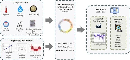
1. Introduction
- For the first time, the historical electrical load data of Pakistan have been considered for the motivation of electric utilities of developing countries to implement machine learning-based STLF methodologies for reliable power system operations.
- To select the input features for the first time from the new unprecedented dataset, the exploratory data analysis, graphical observations and statistical techniques, such as auto-correlation analysis, quantile–quantile analysis and box-plot analysis, are implemented.
- A comprehensive predictor matrix is developed using selected input features for linear and non-linear parametric STLF models. The predictor matrix is not mathematically complex and does not necessarily require data outside the historical patterns.
- This study conducts a comprehensive qualitative and quantitative comparison between the traditional time-series statistical models, linear and non-linear parametric methodologies using several evaluation metrics, such as MAPE, RMSE, MSE, R-square and standard deviation. Moreover, we conducted a thorough seasonal analysis to evaluate and compare the performance of the recommended algorithms.
2. Literature Review
3. Exploratory Data Analysis
3.1. Dataset Description
3.2. Input Parameter Description
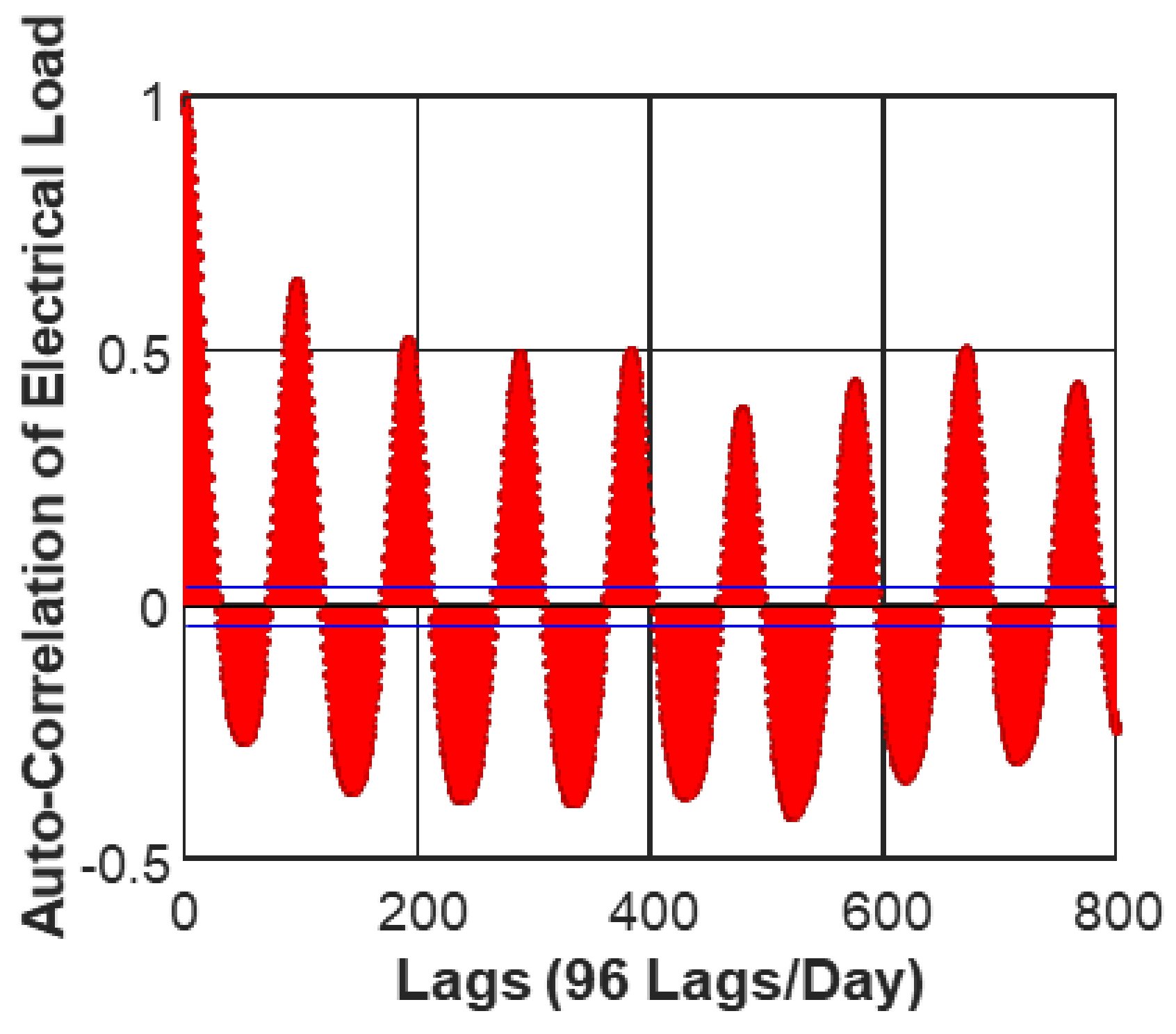
3.2.1. Auto-Correlation Analysis
3.2.2. Quantile–Quantile Plots
3.2.3. Box Plots
4. Methodology
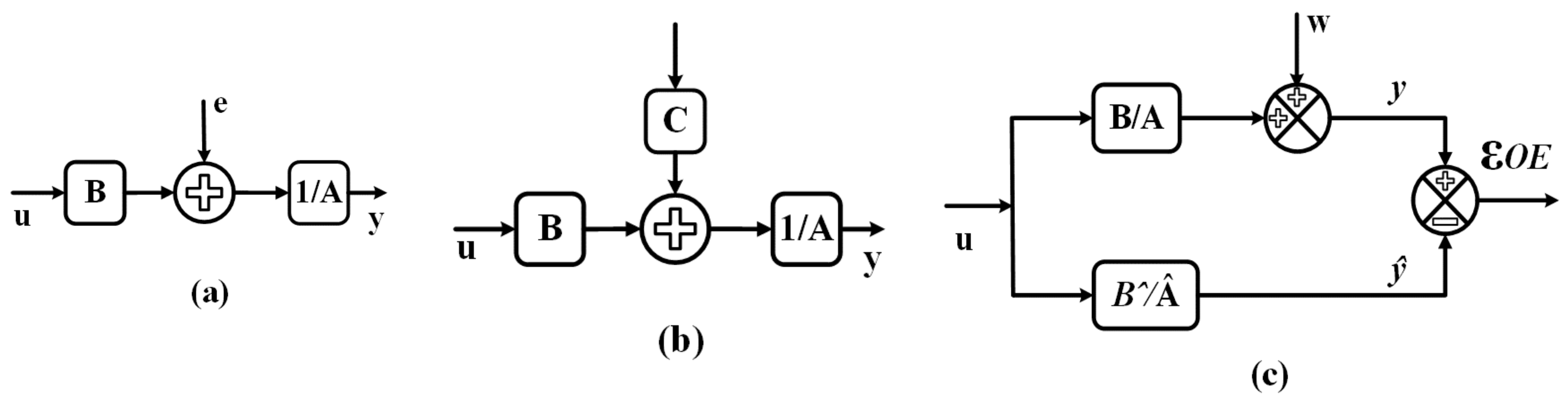
4.1. Auto-Regressive with Exogenous Inputs (ARX)
- ▪
- : the output of process at time ;
- ▪
- : number of poles;
- ▪
- : number of zeros;
- ▪
- : number of input samples that occur before the input affects the output;
- ▪
- : previous outputs on which the current output depends;
- ▪
- previous and delayed inputs on which the current output depends;
- ▪
- : white-noise disturbance value.
4.2. Auto-Regressive Moving Average with Exogenous Inputs (ARMAX)
- ■
- : output at time ;
- ■
- : number of poles;
- ■
- : number of zeroes plus 1;
- ■
- : number of C coefficients;
- ■
- : number of input samples that occur before the input affects the output;
- ■
- : previous outputs on which the current output depends;
- ■
- previous and delayed inputs on which the current output depends;
- ■
- : white-noise disturbance value.
4.3. Output Error Model (OE)
4.4. Support Vector Machine (SVM)
4.5. K-Nearest Neighbour (KNN)
4.6. Bootstrap Aggregation (Bagged Trees)
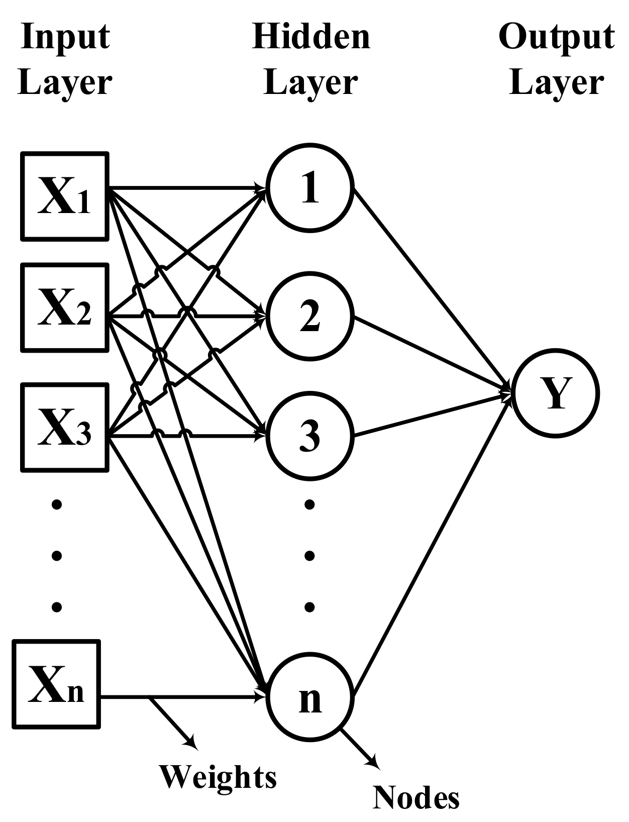
4.7. Artificial Neural Network (ANN)
4.7.1. Particle Swarm Optimization Algorithm (PSO)
4.7.2. Levenberg–Marquardt (LM) Algorithm
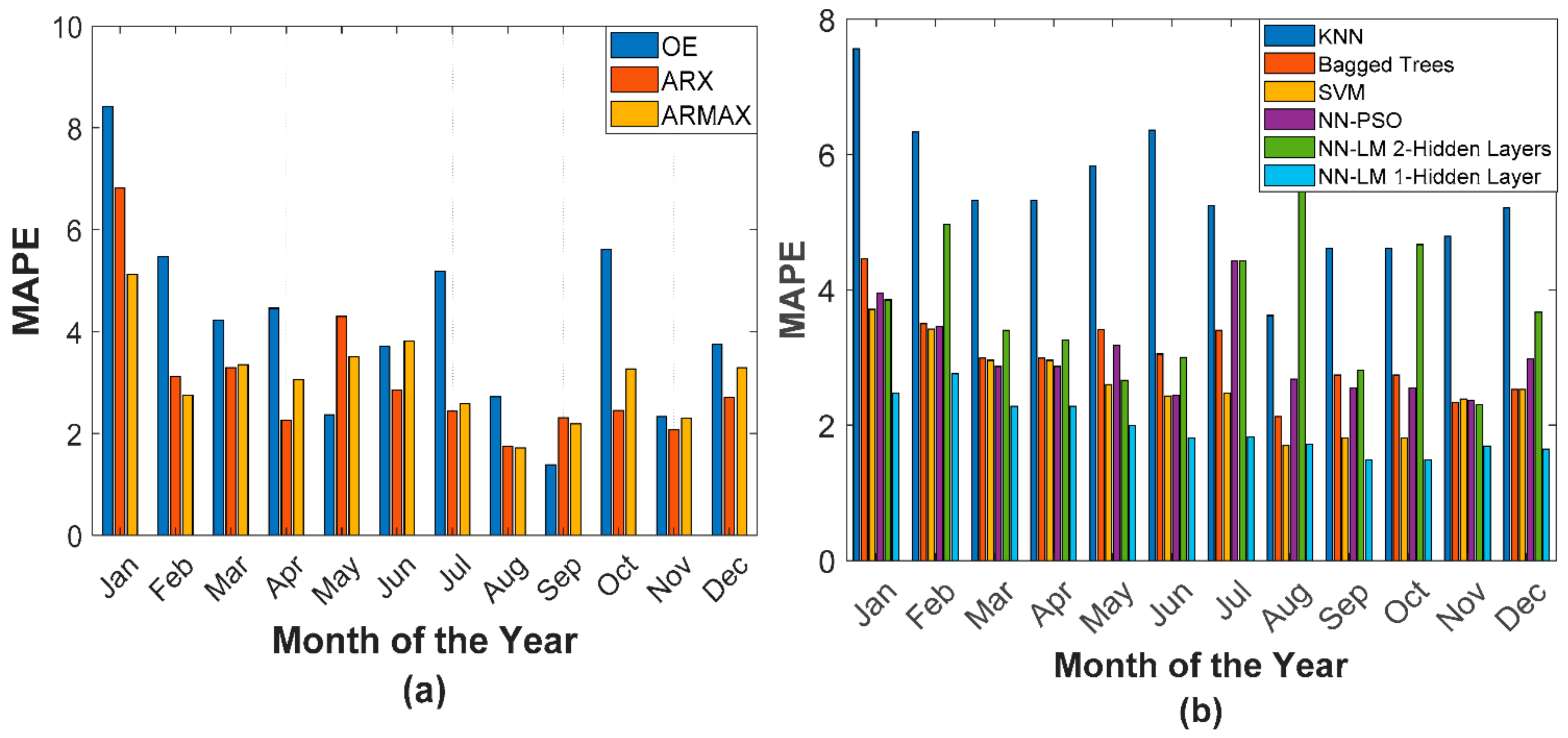
5. Experimental Results and Discussions
5.1. Selection of Evaluation Metrics
5.2. Experimental Background
5.3. Experimental Analysis
- A single layer ANN–LM is different from conventional ANN which uses ANN with regularization parameters. The regularization parameter enables ANN to overcome the overfitting problem.
- A single layer NN–LM improves the training accuracy by using a more advanced optimization algorithm termed as Levenberg–Marquardt (LM).
6. Conclusions
Author Contributions
Funding
Institutional Review Board Statement
Data Availability Statement
Conflicts of Interest
References
- Dudek, G. Short-term load forecasting using neural networks with pattern similarity-based error weights. Energies 2021, 14, 2334. [Google Scholar] [CrossRef]
- Shah, I.; Iftikhar, H.; Ali, S.; Wang, D. Short-term electricity demand forecasting using components estimation technique. Energies 2019, 12, 2532. [Google Scholar] [CrossRef] [Green Version]
- Kiprijanovska, I.; Stankoski, S.; Ilievski, I.; Jovanovski, S.; Gams, M.; Gjoreski, H. HousEEC: Day-ahead household electrical energy consumption forecasting using deep learning. Energies 2020, 13, 2672. [Google Scholar] [CrossRef]
- Jawad, M.; Qureshi, M.B.; Khan, M.U.S.; Ali, S.M.; Mehmood, A.; Khan, B.; Wang, X.; Khan, S.U. A robust optimization technique for energy cost minimization of cloud data centers. IEEE Trans. Cloud Comput. 2021, 9, 447–460. [Google Scholar] [CrossRef]
- Hussain, I.; Ali, S.M.; Khan, B.; Ullah, Z.; Mehmood, C.A.; Jawad, M.; Farid, U.; Haider, A. Stochastic wind energy management model within smart grid framework: A joint bi-directional Service Level Agreement (SLA) between smart grid and wind energy district prosumers. Renew. Energy 2019, 134, 1017–1033. [Google Scholar] [CrossRef]
- Khan, K.S.; Ali, S.M.; Ullah, Z.; Sami, I.; Khan, B.; Mehmood, C.A. Statistical energy information and analysis of Pakistan economic corridor based on strengths, availabilities, and future roadmap. IEEE Access 2020, 8, 169701–169739. [Google Scholar] [CrossRef]
- Wood, A.J.; Wollenberg, B.F.; Sheblé, G.B. Power Generation, Operation, and Control; John Wiley & Sons, Inc.: Hoboken, NJ, USA, 2014; Chapter 12; pp. 566–569. [Google Scholar]
- Jawad, M.; Rafique, A.; Khosa, I.; Ghous, I.; Akhtar, J.; Ali, S.M. Improving disturbance storm time index prediction using linear and nonlinear parametric models: A comprehensive analysis. IEEE Trans. Plasma Sci. 2019, 47, 1429–1444. [Google Scholar] [CrossRef]
- IEA South Asia Energy Outlook 2019. Available online: https://www.iea.org/reports/southeast-asia-energy-outlook-2019 (accessed on 25 August 2021).
- National Transmission and Despatch Company Limited. Power System Statistics 45th Edition. Available online: https://ntdc.gov.pk/ntdc/public/uploads/services/planning/power%20system%20statistics/Power%20System%20Statistics%2045th%20Edition.pdf (accessed on 25 August 2021).
- IEA India Energy Energy Outlook 2021. Available online: https://www.iea.org/reports/india-energy-outlook-2021 (accessed on 25 August 2021).
- Jawad, M.; Ali, S.M.; Khan, B.; Mehmood, C.A.; Farid, U.; Ullah, Z.; Usman, S.; Fayyaz, A.; Jadoon, J.; Tareen, N.; et al. Genetic algorithm-based non-linear auto-regressive with exogenous inputs neural network short-term and medium-term uncertainty modelling and prediction for electrical load and wind speed. J. Eng. 2018, 2018, 721–729. [Google Scholar] [CrossRef]
- Edigera, V.Ş.; Akarb, S. ARIMA forecasting of primary energy demand by fuel in Turkey. Energy Policy 2007, 35, 1701–1708. [Google Scholar] [CrossRef]
- Musbah, H.; El-Hawary, M. SARIMA model forecasting of short-term electrical load data augmented by fast fourier transform seasonality detection. In Proceedings of the IEEE Canadian Conference of Electrical and Computer Engineering (CCECE), Edmonton, AB, Canada, 5–8 May 2019; pp. 1–4. [Google Scholar]
- Dodamani, S.; Shetty, V.; Magadum, R. Short term load forecast based on time series analysis: A case study. In Proceedings of the IEEE International Conference on Technological Advancements in Power and Energy (TAP Energy), Kollam, India, 24–26 June 2015; pp. 299–303. [Google Scholar]
- Yildiz, B.; Bilbao, J.; Sproul, A. A review and analysis of regression and machine learning models on commercial building electricity load forecasting. Renew. Sustain. Energy Rev. 2017, 73, 1104–1122. [Google Scholar] [CrossRef]
- Deb, C.; Zhang, F.; Yang, J.; Lee, S.E.; Shah, K.W. A review on time series forecasting techniques for building energy consumption. Renew. Sustain. Energy Rev. 2017, 74, 902–924. [Google Scholar] [CrossRef]
- Tayaba, U.B.; Zia, A.; Yanga, F.; Lu, J.; Kashif, M. Short-term load forecasting for microgrid energy management system using hybrid HHO-FNN model with best-basis stationary wavelet packet transform. Energy 2020, 203, 117857. [Google Scholar] [CrossRef]
- Jun-long, F.; Yu, X.; Yu, F.; Yang, X.; Guo-liang, L. Rural power system load forecast based on principal component analysis. J. Northeast. 2015, 22, 67–72. [Google Scholar] [CrossRef]
- Bianchi, F.M.; Santis, E.D.; Rizzi, A.; Sadeghian, A. Short-term electric load forecasting using echo state networks and PCA decomposition. IEEE Access 2015, 3, 1931–1943. [Google Scholar] [CrossRef]
- Abu-Shikhah, N.; Elkarmi, F. Medium-term electric load forecasting using singular value decomposition. Energy 2011, 36, 4259–4271. [Google Scholar] [CrossRef] [Green Version]
- Arora, S.; Taylor, J.W. Short-term forecasting of anomalous load using rule-based triple seasonal methods. IEEE Trans. Power Syst. 2013, 28, 3235–3242. [Google Scholar] [CrossRef] [Green Version]
- Shabbir, N.; Kutt, L.; Jawad, M.; Iqbal, M.N.; Ghahfarokhi, P.S. Forecasting of energy consumption and production using recurrent neural networks. Adv. Electr. Electron. Eng. 2020, 18, 190–197. [Google Scholar] [CrossRef]
- Shabbir, N.; Kütt, L.; Jawad, M.; Amadiahanger, R.; Iqbal, M.N.; Rosin, A. Wind energy forecasting using recurrent neural networks. In Proceedings of the Big Data, Knowledge and Control Systems Engineering (BdKCSE), Sofia, Bulgaria, 21–22 November 2019; pp. 1–5. [Google Scholar]
- Ahmed, W.; Ansari, H.; Khan, B.; Ullah, Z.; Ali, S.M.; Mehmood, C.A.A. Machine learning based energy management model for smart grid and renewable energy districts. IEEE Access 2020, 8, 185059–185078. [Google Scholar] [CrossRef]
- Oprea, S.-V.; Bâra, A. Machine learning algorithms for short-term load forecast in residential buildings using smart meters, sensors and big data solutions. IEEE Access 2019, 7, 177874–177889. [Google Scholar] [CrossRef]
- Shirzadi, N.; Nizami, A.; Khazen, M.; Nik-Bakht, M. Medium-term regional electricity load forecasting through machine learning and deep learning. Designs 2021, 5, 27. [Google Scholar] [CrossRef]
- López, M.; Sans, C.; Valero, S.; Senabre, C. Empirical comparison of neural network and auto-regressive models in short-term load forecasting. Energies 2018, 11, 2080. [Google Scholar] [CrossRef] [Green Version]
- Amjady, N.; Keynia, F. A new neural network approach to short term load forecasting of electrical power systems. Energies 2011, 4, 488–503. [Google Scholar] [CrossRef]
- Li, W.; Shi, Q.; Sibtain, M.; Li, D.; Mbanze, D.E. A hybrid forecasting model for short-term power load based on sample entropy, two-phase decomposition and whale algorithm optimized support vector regression. IEEE Access 2020, 8, 166907–166921. [Google Scholar] [CrossRef]
- Mamun, A.A.; Sohel, M.; Mohammad, N.; Sunny, M.S.H.; Dipta, D.R.; Hos, E. A comprehensive review of the load forecasting techniques using single and hybrid predictive models. IEEE Access 2020, 8, 34911–134939. [Google Scholar] [CrossRef]
- Shi, H.; Xu, M.; Li, R. Deep learning for household load forecasting—A novel pooling deep RNN. IEEE Trans. Smart Grid 2018, 9, 5271–5280. [Google Scholar] [CrossRef]
- Fan, G.-F.; Guo, Y.-H.; Zheng, J.-M.; Hong, W.-C. Application of the weighted K-nearest neighbor algorithm for short-term load forecasting. Energies 2019, 12, 916. [Google Scholar] [CrossRef] [Green Version]
- Madrid, E.A.; Antonio, N. Short-term electricity load forecasting with machine learning. Information 2021, 12, 50. [Google Scholar] [CrossRef]
- Román-Portabales, A.; López-Nores, M.; Pazos-Arias, J.J. Systematic review of electricity demand forecast using ANN-based machine learning algorithms. Sensors 2021, 21, 4544. [Google Scholar] [CrossRef] [PubMed]
- Fallah, S.N.; Deo, R.C.; Shojafar, M.; Conti, M.; Shamshirband, S. Computational intelligence approaches for energy load forecasting in smart energy management grids: State of the art, future challenges, and research directions. Energies 2018, 11, 596. [Google Scholar] [CrossRef] [Green Version]
- Velasco, L.C.P.; Estoperez, N.R.; Jayson, R.J.R.; Sabijon, C.J.T.; Sayles, V.C. Day-ahead base, intermediate, and peak load forecasting using k-means and artificial neural networks. Int. J. Adv. Comput. Sci. Appl. 2018, 9, 62–67. [Google Scholar]
- Li, S.; Wang, P.; Goel, L. A novel wavelet-based ensemble method for short-term load forecasting with hybrid neural networks and feature selection. IEEE Trans. Power Syst. 2016, 31, 1788–1798. [Google Scholar] [CrossRef]
- Sun, W.; Zhang, C. A Hybrid BA-ELM model based on factor analysis and similar-day approach for short-term load forecasting. Energies 2018, 11, 1282. [Google Scholar] [CrossRef] [Green Version]
- Zhang, Y.-F.; Chiang, H.-D. Enhanced ELITE-load: A novel CMPSOATT methodology constructing short-term load forecasting model for industrial applications. IEEE Trans. Ind. Inform. 2020, 16, 2325–2334. [Google Scholar] [CrossRef]
- Qiu, X.; Ren, Y.; Suganthan, P.N.; Amaratunga, G.A.J. Empirical mode decomposition based ensemble deep learning for load demand time series forecasting. Appl. Soft Comput. 2017, 54, 246–255. [Google Scholar] [CrossRef]
- Jahan, I.S.; Snasel, V.; Misak, S. Intelligent systems for power load forecasting: A study review. Energies 2020, 13, 6105. [Google Scholar] [CrossRef]
- Turhan, C.; Simani, S.; Zajic, I.; Akkurt, G.G. Performance analysis of data-driven and model-based control strategies applied to a thermal unit model. Energies 2017, 10, 67. [Google Scholar] [CrossRef] [Green Version]
- Jallal, M.A.; González-Vidal, A.; Skarmeta, A.F.; Chabaa, A.; Zerouala, A. A hybrid neuro-fuzzy inference system-based algorithm for time series forecasting applied to energy consumption prediction. Applied Energy 2020, 268, 114977. [Google Scholar] [CrossRef]
- Buitrago, J.; Asfour, S. Short-term forecasting of electric loads using nonlinear autoregressive artificial neural networks with exogenous vector inputs. Energies 2017, 10, 40. [Google Scholar] [CrossRef] [Green Version]
- Bouktif, S.; Fiaz, A.; Ouni, A.; Serhani, M.A. Optimal deep learning LSTM model for electric load forecasting using feature selection and genetic algorithm: Comparison with machine learning approaches. Energies 2018, 11, 1636. [Google Scholar] [CrossRef] [Green Version]
- Komorowski, M.; Marshal, D.C.; Salciccioli, l.D.; Crutain, Y. Secondary Analysis of Electronic Health Records; Springer: Berlin/Heidelberg, Germany, 2016; Chapter 15; pp. 185–203. [Google Scholar]
- Power Information Technology Company. Available online: http://www.pitc.com.pk (accessed on 1 April 2020).
- rp5.ru. Available online: www.rp5.ru/Weather_in_the_world (accessed on 1 April 2020).
- Rajbhandari, Y.; Marahatta, A.; Ghimire, B.; Shrestha, A.; Gachhadar, A.; Thapa, A.; Chapagain, K.; Korba, P. Impact study of temperature on the time series electricity demand of urban nepal for short-term load forecasting. Appl. Syst. Innov. 2021, 4, 43. [Google Scholar] [CrossRef]
- Tudose, A.M.; Picioroaga, I.I.; Sidea, D.O.; Bulac, C.; Boicea, V.A. Short-term load forecasting using convolutional neural networks in COVID-19 context: The romanian case study. Energies 2021, 14, 4046. [Google Scholar] [CrossRef]
- Diversi, R.; Guidorzi, R.; Soverini, U. Identification of ARX and ARARX models in the presence of input. Eur. J. Control. 2010, 16, 242–255. [Google Scholar] [CrossRef]
- Fung, E.H.; Wong, Y.; Ho, H.; Mignolet, M.P. Modelling and prediction of machining errors using ARMAX and NARMAX structures. Appl. Math. Model. 2003, 27, 611–627. [Google Scholar] [CrossRef]
- Schnyer, D.A.M. Machine Learning; Methods and Applications to Brain Disorders; Academic Press: Cambridge, MA, USA, 2020; Chapter 6; pp. 101–121. [Google Scholar]
- Winters-Miner, L.A.; Bolding, P. Practical Predictive Analytics and Decisioning Systems for Medicine; Informatics Accuracy and Cost-Effectiveness for Healthcare Administration and Delivery Including Medical Research; Academic Press: Cambridge, MA, USA, 2015; Chapter 15; pp. 239–259. [Google Scholar]
- Saeed, M.S.; Mustafa, M.W.; Sheikh, U.U.; Jumani, T.A.; Mirjat, N.H. Ensemble bagged tree based classification for reducing non-technical losses in multan electric power company of Pakistan. Electronics 2019, 8, 860. [Google Scholar] [CrossRef] [Green Version]
- Tarkhaneh, O.; Shen, H. Training of feedforward neural networks for data classification using hybrid particle swarm optimization, mantegna lévy flight and neighborhood search. Heliyon 2019, 5, e01275. [Google Scholar] [CrossRef] [PubMed] [Green Version]
- Mathworks. Available online: https://www.mathworks.com/help/deeplearning/ref/trainlm.html (accessed on 15 April 2021).
- Uzair, M.; Jamil, N. Effects of hidden layers on the efficiency of neural networks. In Proceedings of the 2020 IEEE 23rd International Multitopic Conference (INMIC), Bahawalpur, Pakistan, 5–7 November 2020; pp. 1–6. [Google Scholar]


| Meteorological Factors | Temporal Factors | Historical Data |
|---|---|---|
| Temperature | Hour of the Day | Previous Hour Electrical Load |
| Humidity | Day of the Week | Previous Day Same Hour Electrical Load |
| Is it a Working Day? |
| Period (2019) | OE | ARX | ARMAX | KNN | Bagged Trees | SVM | NN–PSO | ANN–LM (Two Hidden Layer) | ANN–LM (Single Hidden Layer) | Errors |
|---|---|---|---|---|---|---|---|---|---|---|
| January | 8.42 | 6.82 | 5.12 | 7.56 | 4.46 | 3.71 | 3.95 | 3.85 | 2.47 | MAPE |
| 142.87 | 120.08 | 92.05 | 136.15 | 80.51 | 65.32 | 71.14 | 70.12 | 44.41 | MAE | |
| 173.14 | 155.08 | 120.25 | 172.14 | 105.12 | 87.08 | 95.42 | 90.94 | 57.96 | RMSE | |
| 0.65 | 0.72 | 0.83 | 0.65 | 0.87 | 0.91 | 0.89 | 0.90 | 0.96 | ||
| 4.61 | 4.18 | 4.31 | 4.89 | 4.40 | 4.87 | 4.81 | 4.91 | 4.87 | Std. Dev. | |
| February | 5.47 | 3.12 | 2.75 | 6.33 | 3.50 | 3.42 | 3.46 | 4.97 | 2.76 | MAPE |
| 92.09 | 53.66 | 47.92 | 109.63 | 58.94 | 58.13 | 60.29 | 84.23 | 47.63 | MAE | |
| 110.57 | 72.15 | 66.10 | 143.71 | 83.81 | 77.19 | 81.73 | 123.62 | 66.33 | RMSE | |
| 0.83 | 0.93 | 0.94 | 0.71 | 0.90 | 0.92 | 0.91 | 0.78 | 0.94 | ||
| 4.84 | 4.78 | 4.92 | 4.87 | 4.54 | 4.66 | 4.60 | 4.94 | 4.66 | Std. Dev. | |
| March | 4.23 | 3.29 | 3.35 | 5.32 | 2.99 | 2.96 | 2.87 | 3.40 | 2.28 | MAPE |
| 77.86 | 60.56 | 61.91 | 100.39 | 55.14 | 54.85 | 52.87 | 62.43 | 42.49 | MAE | |
| 127.84 | 94.33 | 95.23 | 129.94 | 77.47 | 76.48 | 77.88 | 87.49 | 60.54 | RMSE | |
| 0.75 | 0.86 | 0.86 | 0.74 | 0.91 | 0.91 | 0.91 | 0.88 | 0.94 | ||
| 5.16 | 4.51 | 4.70 | 4.23 | 4.39 | 4.53 | 4.57 | 4.35 | 4.53 | Std. Dev. | |
| October | 5.61 | 2.45 | 3.27 | 5.56 | 2.61 | 2.69 | 3.37 | 4.67 | 1.92 | MAPE |
| 125.00 | 55.42 | 72.83 | 126.28 | 58.47 | 59.91 | 75.67 | 106.07 | 43.30 | MAE | |
| 145.49 | 86.89 | 103.54 | 161.38 | 85.10 | 85.89 | 101.08 | 147.06 | 64.47 | RMSE | |
| 0.74 | 0.91 | 0.87 | 0.69 | 0.91 | 0.91 | 0.88 | 0.74 | 0.95 | ||
| 5.16 | 5.11 | 4.92 | 4.97 | 4.98 | 5.11 | 5.30 | 5.38 | 5.11 | Std. Dev. | |
| November | 2.33 | 2.07 | 2.30 | 4.79 | 2.33 | 2.39 | 2.37 | 2.31 | 1.69 | MAPE |
| 42.52 | 38.53 | 42.91 | 88.12 | 43.54 | 44.54 | 44.25 | 43.07 | 31.40 | MAE | |
| 121.26 | 54.34 | 58.60 | 113.30 | 59.01 | 59.66 | 59.66 | 60.27 | 43.90 | RMSE | |
| 0.74 | 0.95 | 0.94 | 0.77 | 0.94 | 0.94 | 0.94 | 0.93 | 0.97 | ||
| 4.64 | 4.30 | 4.29 | 4.36 | 4.21 | 4.25 | 4.35 | 4.26 | 4.25 | Std. Dev. | |
| December | 3.75 | 2.71 | 3.29 | 5.21 | 2.53 | 2.53 | 2.98 | 3.67 | 1.65 | MAPE |
| 63.46 | 47.75 | 57.82 | 92.22 | 44.59 | 44.52 | 51.99 | 64.15 | 29.09 | MAE | |
| 85.93 | 62.62 | 74.29 | 122.25 | 60.64 | 58.16 | 67.83 | 84.84 | 38.26 | RMSE | |
| 0.90 | 0.95 | 0.93 | 0.80 | 0.95 | 0.96 | 0.94 | 0.91 | 0.98 | ||
| 5.59 | 4.72 | 4.56 | 4.92 | 4.74 | 4.84 | 4.73 | 4.89 | 4.84 | Std. Dev. |
| Period (2019) | OE | ARX | ARMAX | KNN | Bagged Trees | SVM | NN–PSO | ANN–LM (Two Hidden Layer) | ANN–LM (Single Hidden Layer) | Errors |
|---|---|---|---|---|---|---|---|---|---|---|
| April | 4.46 | 2.26 | 3.05 | 6.49 | 3.58 | 2.98 | 2.64 | 3.26 | 2.24 | MAPE |
| 105.40 | 53.03 | 72.20 | 153.69 | 79.79 | 68.90 | 59.49 | 76.41 | 52.98 | MAE | |
| 258.59 | 108.92 | 119.80 | 206.89 | 132.18 | 111.25 | 94.67 | 103.62 | 76.53 | RMSE | |
| 0.50 | 0.91 | 0.89 | 0.68 | 0.87 | 0.91 | 0.93 | 0.92 | 0.96 | ||
| 7.82 | 6.48 | 6.54 | 5.36 | 6.06 | 6.33 | 6.33 | 6.55 | 6.33 | Std. Dev. | |
| May | 2.37 | 4.30 | 3.50 | 5.83 | 3.41 | 2.60 | 3.18 | 2.66 | 1.99 | MAPE |
| 72.45 | 123.04 | 104.10 | 180.37 | 104.95 | 76.89 | 97.64 | 82.61 | 61.28 | MAE | |
| 104.58 | 180.15 | 160.74 | 234.70 | 152.99 | 118.70 | 143.03 | 113.82 | 84.12 | RMSE | |
| 0.93 | 0.78 | 0.83 | 0.64 | 0.85 | 0.91 | 0.87 | 0.92 | 0.95 | ||
| 6.60 | 6.82 | 6.58 | 6.17 | 5.95 | 6.74 | 6.17 | 6.47 | 6.74 | Std. Dev. | |
| June | 3.71 | 2.86 | 3.82 | 6.36 | 3.05 | 2.43 | 2.44 | 3.00 | 1.81 | MAPE |
| 120.38 | 90.67 | 122.98 | 209.54 | 99.10 | 75.53 | 79.60 | 98.41 | 58.77 | MAE | |
| 186.74 | 143.48 | 171.35 | 269.87 | 152.86 | 130.70 | 113.97 | 126.41 | 82.45 | RMSE | |
| 0.75 | 0.85 | 0.79 | 0.48 | 0.83 | 0.88 | 0.91 | 0.89 | 0.95 | ||
| 6.67 | 6.26 | 5.96 | 5.63 | 5.67 | 6.33 | 6.34 | 5.99 | 6.33 | Std. Dev. | |
| July | 5.19 | 2.44 | 2.59 | 5.24 | 3.40 | 2.48 | 4.43 | 4.43 | 1.82 | MAPE |
| 178.29 | 77.40 | 82.01 | 170.63 | 112.84 | 77.61 | 151.55 | 148.24 | 59.70 | MAE | |
| 217.83 | 141.37 | 148.72 | 242.24 | 177.35 | 144.56 | 205.33 | 197.60 | 95.08 | RMSE | |
| 0.73 | 0.89 | 0.87 | 0.67 | 0.82 | 0.88 | 0.76 | 0.78 | 0.95 | ||
| 9.19 | 7.45 | 7.30 | 6.25 | 6.47 | 7.39 | 6.38 | 7.23 | 7.39 | Std. Dev. | |
| August | 2.72 | 1.75 | 1.72 | 3.62 | 2.13 | 1.70 | 2.68 | 5.91 | 1.72 | MAPE |
| 90.93 | 57.95 | 56.84 | 123.59 | 72.35 | 56.22 | 88.81 | 204.76 | 57.19 | MAE | |
| 126.50 | 95.93 | 99.05 | 165.82 | 110.31 | 92.61 | 133.20 | 253.36 | 90.37 | RMSE | |
| 0.84 | 0.91 | 0.90 | 0.73 | 0.88 | 0.92 | 0.82 | 0.37 | 0.92 | ||
| 5.39 | 5.30 | 5.48 | 4.79 | 5.06 | 5.45 | 4.95 | 3.20 | 5.45 | Std. Dev. |
Publisher’s Note: MDPI stays neutral with regard to jurisdictional claims in published maps and institutional affiliations. |
© 2021 by the authors. Licensee MDPI, Basel, Switzerland. This article is an open access article distributed under the terms and conditions of the Creative Commons Attribution (CC BY) license (https://creativecommons.org/licenses/by/4.0/).
Share and Cite
Javed, U.; Ijaz, K.; Jawad, M.; Ansari, E.A.; Shabbir, N.; Kütt, L.; Husev, O. Exploratory Data Analysis Based Short-Term Electrical Load Forecasting: A Comprehensive Analysis. Energies 2021, 14, 5510. https://doi.org/10.3390/en14175510
Javed U, Ijaz K, Jawad M, Ansari EA, Shabbir N, Kütt L, Husev O. Exploratory Data Analysis Based Short-Term Electrical Load Forecasting: A Comprehensive Analysis. Energies. 2021; 14(17):5510. https://doi.org/10.3390/en14175510
Chicago/Turabian StyleJaved, Umar, Khalid Ijaz, Muhammad Jawad, Ejaz A. Ansari, Noman Shabbir, Lauri Kütt, and Oleksandr Husev. 2021. "Exploratory Data Analysis Based Short-Term Electrical Load Forecasting: A Comprehensive Analysis" Energies 14, no. 17: 5510. https://doi.org/10.3390/en14175510
APA StyleJaved, U., Ijaz, K., Jawad, M., Ansari, E. A., Shabbir, N., Kütt, L., & Husev, O. (2021). Exploratory Data Analysis Based Short-Term Electrical Load Forecasting: A Comprehensive Analysis. Energies, 14(17), 5510. https://doi.org/10.3390/en14175510