Design and Modeling of Metallic Bipolar Plates for a Fuel Cell Range Extender

Abstract

Fuel cells, designed for mobile applications, should feature compact and low-weight designs. This study describes a design process that fulfills the specific needs of target applications and the production process. The key challenge for this type of metallic bipolar plate is that the combination of two plates creates three flow fields, namely an anode side, a cathode side, and a coolant. This illustrates the fact that each cell constitutes an electrochemical converter with an integrated heat exchanger. The final arrangement is comprised of plates with parallel and separate serpentine channel configurations. The anode and cathode sides are optimized for operation under dry conditions. The final plate offers an almost perfect distribution of coolant flow over the active area. The high quality of this distribution is almost independent of the coolant mass flow, even if one of the six inlet channels is blocked. The software employed (OpenFOAM and SALOME) is freely available and can be used with templates.

1. Introduction

Battery- and fuel cell-powered vehicles have attracted increasing attention during the last decade [1,2,3,4,5,6,7,8]. They offer an alternative to internal combustion engines which are primarily based on the consumption of fossil fuels. From the technological point of view, battery-powered vehicles are advantageous for short driving ranges up to 160 km [9]. This number may be taken as a rough guideline, as in real world applications, other terms, such as the availability of a charging infrastructure [10] and prices for competing transport solutions [8,11], are also important. All of these criteria strongly affect the social acceptance of electric vehicles, as shown by Burkert et al. [12] in their analysis of Germany from 2011 to 2020.

In order to increase the driving range, a battery system can be combined with a fuel cell. The term ‘fuel cell vehicle’ is commonly used for hybrid systems in which the the main power is delivered by the fuel cell system, and the battery is merely used to cover highly dynamic load changes [13]. In the case of a range extender, the fuel cell system mainly operates as a more or less constant charging unit for the battery, which acts as the primary power unit. The main challenge for such range extenders is to provide extra power without adding significantly to the complexity of the fuel cell system. Furthermore, this should come at low additional costs in terms of payload and sale price.

Recently, a number of commercial cars have been released as battery-powered models with a polymer electrolyte fuel cell system used for range extension. Among these, the Renault Kangoo was presented in 2015 and uses a 5 kW fuel cell system [14,15]. Another example is the Fiat 500 passenger car equipped with a 30 kW fuel cell system [16,17,18]. In order to reduce weight, the system operates on dry air and hydrogen and employs the anodic recirculation of product water. As a special application for utility vehicles, the company Proton Motor introduced a 7 kW range extender [16,19] with the main goal of reducing the required battery size. Despite these highly successful demonstrations, there remain some issues to be resolved. One of the major goals is the further reduction of costs for the range extender, as a competitive selling price is always a key target for emerging technologies. This issue is addressed by the CoBIP project, in which the mass production of metallic bipolar plates in a role-to-role process is developed [20]. The goal of the project is the production of a modular 24 kW system for a light-duty commercial vehicle [21], as displayed in Figure 1. The fuel cell system will be mounted on the roof of a battery-powered car. The figure shows a system consisting of four stacks, a high-pressure hydrogen tank, and heat exchangers. The rooftop position favors a flat and light-weight design. The fuel cells will be operated without additional humidifier in order to reduce the system’s weight and complexity.

The overall production process combines the techniques of calendering, laser welding, laser cutting, coating, and stack assembly. Each production step adds some requirements to the final flow field plates, as summarized by Porstmann et al. [22]. In general, there are two different design options for bipolar plates, which depend on the plate material. There are compact plates (mostly graphitic) where structures may be milled or thin metallic plates which can be stamped [22,23]. For graphitic plates, it is possible to design the flow fields for anode, cathode and coolant more or less independently. In the case of plates made from thin metal sheets, it is possible to integrate cooling into the plate design of the anode and cathode. 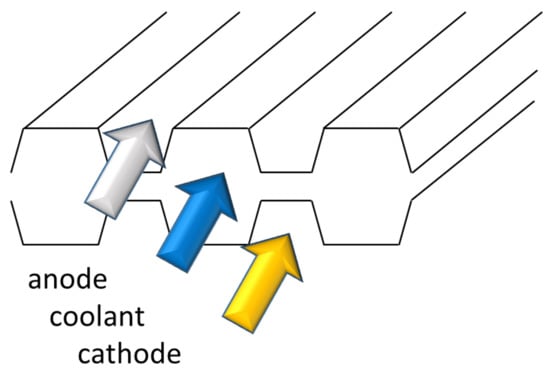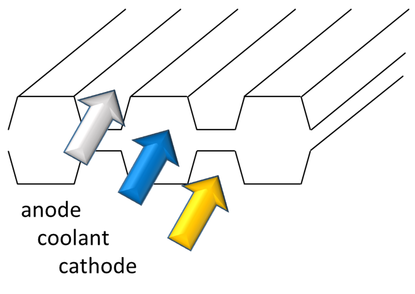Here, each plate defines the gas flow field on one side and half of the coolant flow field on the back side [23,24,25]. The final cell plate consists of an anode plate and a cathode plate welded together and is, therefore, called a double-plate concept. This adds additional complexity to the overall design process, as the combination of two plates yields three different flow fields. Figure 2 shows a cross section of such an arrangement and aptly demonstrates that the final arrangement is highly compact and features a high utilization of the available space.

In the literature, a vast number of different flow field designs exist that may be used in polymer electrolyte fuel cells. In general, a few basic flow field types, such as parallel, pin type, serpentine, interdigitated, and wave, may be distinguished, which are discussed, amongst other topics in the reviews of Li and Sabir [24], Kahraman and Orhan [26], Sauermoser et al. [27], and Wilberforce et al. [28]. These basic types can be modified according to the specific needs of the target application. A recent review by Çelik et al. lists 33 modified flow field designs [29] for performance enhancement. Manso et al. analyzed the influence of the geometric parameters on the performance of PEFCs in their review [30]. A major problem for such a comparison is that the operating conditions for each original study can significantly differ [30]. Therefore, it is important to separately consider each cell design within the context of its application. As a general statement, it can be concluded that serpentine and interdigitated designs usually achieve a more uniform reactant distribution [30]. The counter flow configuration of anode and cathode show better membrane hydration, thus increasing the overall cell performance [30]. A ratio of channel/rib $<1$ is advantageous for operation at lower current densities, and a ratio of channel/rib $>1$ shows better performance at higher current densities [30,31,32]. In order to improve the performance of particular flow field types, several optimization strategies have been reported. Liu and Wang reported a coupled modeling and experimental testing procedure for PEFCs with a very wide channel within a single serpentine configuration [33]. Under the given operating conditions, a channel/rib ratio close to unity was obtained, namely a channel width of 1.0 mm and a rib width of 0.8 mm. Ghanbarian et al. investigated parallel serpentine flow fields with different number of channels [34]. They also concluded that a channel/rib ratio of unity is the best option. For small channels with a width < 1 mm, Cooper et al. [35] found that not only the ratio of channel/rib is important, but also the hydraulic diameter. By applying a design of experiments approach, they found an optimum for hydraulic diameters in the range of 0.40 to 0.45 mm. Limjeerajarus and Charoen-amornkitt [36] compared in their numerical study a small test cell with serpentine and straight channel arrangements. They demonstrated the importance of a proper flow distribution over the active area, especially if the channels of a straight parallel flow field are supplied by a single channel as a distributor. It is a common feature of all flow fields with multiple channels that the flow must be distributed as evenly as possible from an inlet pipe to the separate channels. This topic is addressed in the works of Ramos-Alvarado et al. [37] and Lim et al. [38] regarding straight channel flow fields. They show that it is possible to distribute the flow from a smaller inlet area by introducing suitable distributor structures within the active cell area. The performance can be further optimized by changing the shape of the channel cross section, as described by Wang et al. [39] for triangles, semicircles, and trapezoidal shapes [39,40]. It is also possible to use drilled in holes in a through plane array [41] or straight channels with bulges [42] or indentations [43]. Finally, the flow field can also be composed of a fine mesh, as shown for the Toyota fuel cell system [1,44].

The discussion thus far has mainly been derived from single cell experiments, in which active cooling is not required. The assembly of several cells into a stack raises the need to remove excess heat. There are several techniques that can be chosen for the cooling of a PEFC system. The reviews of Zhang and Kandlikar [45], Bargal et al. [46], and Li et al. [47] provide a comprehensive overview of this topic. The simplest method is so called ‘passive cooling’, which makes use of the high heat conductivity of the flow field plate material. This method is primarily used for devices with smaller power outputs [45]. An ‘active cooling’ system, in contrast, refers to one in which a fluid is actively pumped through a separate cooling flow field. The fluid can be air, but, for higher power densities, a liquid coolant is typically used because the heat transfer is more effective for a liquid with the same pumping power [45]. An even higher cooling effect can be achieved, if the heat of evaporation of a liquid is used instead of heat transfer to a fluid [48]. A deeper discussion, together with an optimization strategy of the channel shape for evaporative cooling, can be found in the work of Soupremanien et al. [49]. A well known application of this principle can also be found in heat pipe devices, as demonstrated by Clement and Wang [50] and Supra et al. [51,52] in their studies for fuel cell applications. Each of these cooling technologies increases demands on the construction of the fuel cell stack. In this paper, cooling with a liquid is considered, as this technique offers the highest compactness for the integrated design shown in Figure 2. The application of a liquid coolant, in turn, requires the existence of a coolant flow field. An obvious solution to this is to use a similar approach as in the flow fields discussed above for the distribution of hydrogen and air [45,46]. Again, many different variants of these flow fields are discussed in the literature. The main purpose of the coolant flow field is to generate a desired temperature profile across the active area. In most cases, homogeneous temperature distribution is preferred, which can be experimentally verified through the use of infrared thermography [53]. A special approach is to utilize metal meshes or foams for the coolant flow field. Afshari et al. compared these with straight channel and serpentine arrangements [54]. The metal foam exhibits improved heat transfer facilitated by the larger inner surface at the price of an increased flow resistance. The approaches that have been discussed thus far require a separate coolant flow field; in many cases, this means a separate cooling cell, such as an internal heat exchanger. Matsunaga et al. (Honda) [55] presented a different solution that is especially suitable for the application of thin metal plates (see Figure 2). The flow channels exhibit a wave-like pattern that allows the coolant to pass through on the back side.

In most of the cited literature, the design of the flow field is performed with the goal of improving fuel cell performance. This is a challenging task, as such, as there are many physical processes to be considered that are all directly or indirectly coupled. The work of Alaswad et al. [56] provides a good overview of the influence of operating parameters on fuel cell performance. Performance can, in turn, only be measured if a working fuel cell already exists. The focus of this work is to derive a design strategy for the initial step of flow plate design. Many parameters arise from the manufacturing process that must be taken into account, and which have a high impact or imply severe constraints on the overall design. The novelty of this work is the development of such a design process that allows the creation of two bipolar plates and, respectively, three flow fields, in one design step. It is demonstrated how the large number of influencing parameters can be incorporated by an effective modeling approach. The impact of uncertainty on the modeling results is investigated, and the consequences for the final results are discussed. A toolbox is provided in the supplementary material which assists in the automated design screening steps.

2. Methodology

There are, in principle, two possible approaches to the development of fuel cell plates. The ‘bottom up’ method starts with an existing flow field for a single cell or short stack. This initial design is modified in the following steps to meet the requirements of the final system. The main advantage of this strategy is that, despite the overall complexity of the system, the result is always a working fuel cell. The overall process can be understood as an optimization procedure, whose success depends on the ability to overcome the critical restrictions that may be inherited from the starting design. The second approach is the ‘top down’ method that is followed in this work. As the first step, the requirements deriving from the target application and the production process are collected. Based on these, an overall concept is derived. Finally, the single plates are designed and evaluated. The major advantage of this approach is that the resulting fuel cell is guaranteed to meet all of the requirements. The main risk for the final product lies in the ability to develop a working fuel cell with a large number of constraints. There is a chance that the final fuel cell must go through an additional optimization step in order to reach the desired performance.

2.1. Requirement Specification

It can be determined from the target application as a range extender (see Figure 1) that the flow field plates should have a low weight and an overall flat shape. Therefore, it was decided to produce the plates from thin metal sheets (stainless steel: 0.1 mm) by means of a calendering process. The plates will be further processed by laser cutting and welding. All production steps can be integrated into a lean production line. The final step in this line will be the assembly of the fuel cell stacks. At this point, two sets of requirements must be defined. Firstly, the design of the system imposes operational requirements. These result from the nominal power output, the size of the blowers and pumps, and possibly the recirculation system. Secondly, each production step can impose specific restrictions. These may include the channel geometry from the calendering process or the spatial demand for welding. All of the requirements are listed in

Table 1. Requirements for the range extender plates.

Parameter	Value	Comment
Operation temperature	60 ${}^{\circ }$C to 70 ${}^{\circ }$C
$\Delta T$ from inlet to outlet	2.5 K to 10.0 K
Total current	min. 18 A and max. 44 A
Geometric active cell area	100 cm${}^2$	5 cm by 20 cm
Number of cells in stack	approx. 200
Cathode gas	ambient air	no humidification
Anode gas	78.7 Vol% H${}_2$, 12.5 Vol% H${}_2$O, 8.8 Vol% N${}_2$	recirculation
Coolant	commercial glycol type
Stoichiometric coeff.	anode = 2.0 and cathode = 2.0
Cathode $\Delta p$	≤0.18 bar
Anode $\Delta p$	≤0.07 bar
Coolant $\Delta p$	≤0.30 bar
Flowfield	different for anode and cathode	different mass flow and $\Delta p$
Channel depth	≤0.4 mm	from calendering
Inclination (channel wall)	${15}^{\circ }$	from calendering
Channel bottom width	≥0.7 mm	from laser welding

. The targeted current density is very low for a PEFC system, which leads to operating points at a high level of cell efficiency. The expected cell voltage is $\ge 0.7$ V, and a single stack will contain approximately 200 cells. The nominal power output of a single stack is about 2.5–6.2 kW, and the whole system incorporates four stacks.

Another geometric requirement for the flow field plates is that the internal structure must match the arrangement of the stack manifolds. In principle, there are two possible arrangements of the stack manifolds, as is shown in Figure 3. It is obvious that the arrangement in Figure 3a, with the coolant manifolds on the sides, will require more space. From the target application, a maximum compactness is desired. Therefore, the solution presented in Figure 3b is chosen. A similar arrangement was also followed in the works of Janßen et al. [25], Giacoppo et al. [57], and Asanin [43]. This choice adds a further geometric constraint to the head and tail region of the cell, wherein the flow of the three fluid regions for the anode, cathode, and coolant must be spread out as evenly as possible over the active area and re-collected at the end into the outlet manifolds.

At this point, another decision should be taken: the main flow configuration of the coolant. The coolant can either be distributed in flow direction with hydrogen and air or in cross-flow configuration, as depicted in Figure 4.

It must be guaranteed that the coolant is able to flow from inlet to outlet. Therefore, blockages may only occur on one plate, but not at both anode and cathode plates at the same position. For the co-flow configuration from Figure 4a, the channels of the anode and cathode plate should be mostly straight, superimposable and have little perpendicular blocking in the main flow direction. This concept has the advantage that a desired temperature gradient can be generated or compensated for by leading the coolant in co-flow or counter-flow direction. For the cross-flow configuration in Figure 4b, the channels must not be superimposable. A wave-like pattern would be advantageous, as discussed by Matsunaga et al. [55], for the HONDA FCX Clarity system. This choice also leads to the need to distribute the coolant from the broad side, which would, in turn, be more suitable for the manifold configuration shown in Figure 3a. The cross-flow configuration in blocks (Figure 4c) is, in principle, a variation of Figure 4b that combines the idea of cross-flow at the level of channels while effectively leading the coolant in co-flow or counter-flow with hydrogen and air.

The choice of the preferred channel configuration for thin metal plates should be further influenced by considering mechanical stability and electric conductivity. In the center of Figure 2, it can be seen that the two plates of anode and cathode are connected at the bottom of the channels. The overall size of the area for conducting the current depends on the relative position of the channel bottom on anode and cathode plates. It is further influenced by the shape of the channel cross section, which is trapezoidal for stamping processes and on the width ratio of channel and rib. Figure 5 summarizes three common channel configurations. For the resulting contact area, the following trend can be derived if one assumes a rectangular channel cross-section and a channel/rib ratio of unity. In the case the of straight parallel flow fields from Figure 5a, the maximum contact area is 50% of the geometric cell area. For a cross-flow configuration, such as that in Figure 5b, the contact area can only be 25%. For wave-like channels, the value depends on the curvature, but it should tend more towards 25%. These numbers will decrease if the flatness of the channel bottom is imperfect.

Thus far, a fairly large number of requirements and constraints have been outlined. Depending on the point of view, these can be perceived in terms of either an ‘endless list of problems’ or as a ‘list of wishes that are nice to have’. It is almost impossible to consider all of these parameters at the same time. In order to proceed in the design process, a priority list should be compiled as shown in the following.

• Compact design with an overall flat shape.
• Channel depth $\le 0.4$ mm.
• Stack manifolds in the head and tail positions (see Figure 3b).
• Co-flow configuration for anode, cathode and coolant (see Figure 4a).
• Straight, superimposed channels rather than wave-like (see Figure 5a).
• Channel bottom width $\ge 0.7$ mm.
• The cell plates should consist of an anode and cathode plate, i.e., different flow fields for anode and cathode sides.
• Channel/rib ratio = unity.
• Geometry of the active area = 5 cm by 20 cm.

From the list above, it is clear that the decision is dominated by the positioning of the manifolds. Therefore, flow configurations with mostly straight channels should be considered during the initial design process.

2.2. Computational Fluid Dynamics Simulation

Computational fluid dynamics (CFD) models of fuel cells are powerful tools for design optimization and fault diagnostics. The accuracy of these models strongly depends on a large number of parameters and submodels originating from the complex nature of the underlying physical processes. The validation of these parameters usually depends on a specific design.

For the screening process of new designs, a strongly simplified ’fuel cell model’ has been used. The electrochemical reaction is mimicked as a constant mass sink/source at the interface of the porous transport layer (gas diffusion layer (GDL)) to the catalyst layers. Simulations are carried out for the anode and cathode plates separately. The sketch shown in Figure 6 demonstrates this configuration. The result of such simulations is an estimation of the pressure differences and the general flow distribution along the channels, as well as under the land area. These results are not intended to give exact numbers, but they are useful as first estimates. Furthermore, different channel configurations can be compared, and the overall quality of the flow distribution can be assessed. The correct distribution of water vapor between cathode and anode side depends on the local osmotic drag factor and water back diffusion through the membrane. A forward prediction of the water distribution is very challenging, even for advanced fuel cell models. Therefore, the model does not consider the consumption of species but, rather, solves the balance of mass instead. All product water is attributed to the cathode side, where the consumption of oxygen and the production of water vapor lead to an influx of fluid at the interface of the GDL (see Figure 6). On the anode side, the consumption of hydrogen is simulated by an outlet condition. All results were obtained under the assumption that the diffusion of hydrogen and oxygen is fast enough to avoid local depletion.

The properties of the GDL are shown in Table S1 (in the supplementary) and consist of averaged values for typical GDL materials [58,59]. The choice of these parameters comes with a high degree of uncertainty, as these values depend on the specific material, which was not defined at the beginning of the screening process. Furthermore, the effects of local compression under the land area and intrusion into the channel are not explicitly considered. A variation in the specific permeability will lead to a modification of the total pressure difference. It was shown in a previous study by Reimer et al. [60] that there exist two different scenarios. As long as the channel depth is larger than the GDL thickness, the impact of permeability on $\Delta p$ is low. If the channel depth is smaller, the main flow must pass more through the GDL, and the impact on $\Delta p$ can be significant. For the present plate design, the situation may fall just in between these two scenarios.

The parameters for the channel geometry and the properties of the porous transport layer will be affected by the presence of liquid water. Therefore, it is useful to estimate the expected amount of liquid water during fuel cell operation. As shown in Table 1, dry air is used for the cathode side. The anode off gas will then be partially recirculated. Therefore, it will contain a small amount of nitrogen, which diffuses to some extent from the cathode side via the membrane because of the large concentration gradient. The anode gas mixture is assumed to exhibit 50% relative humidity at the inlet of the anode side (at 65 ${}^{\circ }$C) and about 100% relative humidity at the outlet, as the stoichiometry coefficient for hydrogen is two. The product water can be attributed to the cathode side as initial assumption. Table S2 (in the supplementary) summarizes the molar fluxes on the cathode side for this consideration. It follows that the molar fraction of water will be $X_{H_{2}O}=0.19$ at the cathode outlet. As the saturation value is $X_{H_{2}O}^{sat}=0.25$, the exhaust air would leave the cell with a relative humidity of 76% at 65 ${}^{\circ }$C. This indicates that, overall, no liquid water needs to be removed, although the actual water distribution may differ. By following these considerations, the critical amount of water at the cathode inlet can be calculated, which would lead to the formation of liquid water at the outlet of the cell. In order to reach the saturation limit at the outlet, the inlet air stream must contain a value of $0.95\times {10}^{-4}$ mol s${}^{-1}$ of water, which corresponds to the condition of 100% relative humidity at 42 ${}^{\circ }$C.

Table 2. Fluid properties at 65 ${}^{\circ }$C for the CFD simulations.

Parameter	Cathode	Anode	Coolant
Density/kg m${}^{-3}$	1.04	0.23	$1.05\times {10}^3$
Dyn. viscosity/Pa s	1.80 $\times {10}^{-5}$	1.80 $\times {10}^{-5}$	$1.35\times {10}^{-3}$
Kin. viscosity/m${}^2$ s${}^{-1}$	$1.73\times {10}^{-5}$	$7.94\times {10}^{-5}$	$1.29\times {10}^{-6}$

summarizes the properties of all fluids used in the simulations. The fluid used as a coolant is assumed to be a mixture of 50% glycol and 50% water with a heat capacity of $c_p=3.46$ kJ kg${}^{-1}$ K${}^{-1}$.

The CFD simulations were carried out using the free software package OpenFOAM [61,62]. For geometry and mesh generation, the toolbox of Reimer et al. [60] was employed, which relies on the free software SALOME [63] and generates flow fields for half cell configurations, i.e., channels and porous transport layer. The toolbox was extended to automatically generate the three different channel configurations shown in Figure 7. These examples are also documented in the supplementary information of this study. The serpentine shapes were chosen because they provide good under the rib convection as a result of the pressure difference of adjacent channel sections [64,65,66,67]. A detailed description of the pressure differences for the separate serpentine flow field can be found in the PhD thesis of Bendzulla [68].

The following parameters can be set for the scripted flow field generation.

• Width and height of channels.
• Height of GDL.
• Number of channels.
• Total width of flow field.
• Length of additional inlets and outlets.
• Width of the serpentines and number of U-turns.
• Mesh resolution of the channels and GDL.

The geometric model considers channels with rectangular cross sections rather than the trapezoidal shape depicted in Figure 8. This choice was made in order to reduce the model complexity. A more in depth discussion can be found in the study by Reimer et al. [60]. In summary, the model uses a rectangular cross section which features the same hydraulic diameter as the ‘real channel’. To accomplish this constraint, the width of channel and land were kept identical, and the channel depth of the model was adjusted accordingly. Furthermore, the exact angle of the channel walls will be a result of the final production process [22,40,69]. For the design, a value of $\alpha ={15}^{\circ }$ is used.

The overall procedure of the design process can be summarized by the following steps.

• Specification of the channel cross section.
• Screening of the flow field geometries for straight channel configuration, parallel serpentines and separate serpentines.
• Calculation of $\Delta p$ for selected flow field geometries.
• Selection of favorable combinations for anode and cathode sides with respect to the resulting coolant flow field.
• Adding manifold regions to the coolant flow field and calculation of $\Delta p$ for the coolant.

3. Results and Discussion

The content of this study focuses on the design of the flow field itself. The design of the plates is more complex because it also includes considerations from sealing, stack assembly, and the design of the cell manifolds. The description of the design process in this study is strongly idealized in order to highlight the major points. Typically, the overall process is not straightforward.

3.1. Channel Cross Section

Initially, a suitable channel cross section must be selected. Based on the requirements listed in Table 1, the following choice has been made for the trapezoidal channel (see Figure 8): $w1=0.90$ mm, $h=0.36$ mm, and $w2=0.72$ mm. The resulting hydraulic diameter is $d_h=0.49$ mm. The width of $w2$ is sufficient for the requirement from laser welding, and the hydraulic diameter is close to the optimal as reported by Cooper et al. [35] ( $d_h=0.40$ to 0.45 mm). For the CFD simulation, a rectangular cross section of $w1=0.90$ mm and $h^{\ast }=0.34$ mm results to yield the same value for $d_h$.

Overall, it can be said that the cross section of the channel is very small. With respect to the production process, it has to be expected that the outline of the channel will show some variation in height. In order to explore the impact on the CFD simulations, the height variation was assumed to be $\pm 0.05$ mm. This rather large value was also chosen to account for the uncertainty of the properties of the GDL material, as it influences the ratio of flow through the porous material and the channel. A more detailed discussion of the intrusion of the porous material into the void space of the channel caused by production tolerances can be found in the work of Hoppe et al. [70].

Table 3. Channel dimensions for the CFD simulation with a variation of $\pm 0.05$ mm in depth. For the parameters, see Figure 8.

	Trapezoidal	Rectangular
h/mm	0.360	0.338
$w_1$/mm	0.900	0.900
$w_2$/mm	0.707	–
$d_h$/mm	0.492	0.492
h/mm	0.410	0.379
$w_1$/mm	0.900	0.900
$w_2$/mm	0.680	–
$d_h$/mm	0.533	0.533
h/mm	0.310	0.296
$w_1$/mm	0.900	0.900
$w_2$/mm	0.734	–
$d_h$/mm	0.445	0.445

presents the cross sections used for the simulations.

The trapezoidal shape also has a severe impact on the back-to-back contact area between two plates (see Figure 2). In order to demonstrate this effect, a flow field with straight channels will be considered. In this work, the width of the active area is considered to be equal to the maximum distance from the first channel to the last, i. e., a 30-channel configuration would span 30 times the channel width plus 29 times the land width. For a flow field with equal channel and rib widths, a contact area of 51% of the geometrically active area would result. For a flow field with trapezoidal shaped channels with $w_1=0.900$ mm and $w_2=0.707$ mm (see Table 3), a contact area of 40% results.

3.2. Mesh Dependency

The fluid flow must pass through the porous GDL, as well as through the gas channels. The depth of the channel and the thickness of the GDL are almost identical in this work. This indicates that the resolution of the computational mesh needs to be fine enough to capture the right balance of flow distribution between these two domains. For the mesh dependency study, a four channel parallel serpentine flow field was chosen with an active area of 10 cm${}^2$.

Table 4. Mesh configurations for a geometric area of 10 cm${}^2$ with a channel width of 0.9 mm.

Name	E7	E9	R8	R12	R16	R20
Channel resolution	$7\times 4$	$9\times 5$	$8\times 6$	$12\times 8$	$16\times 10$	$20\times 14$
Mesh cells	0.4 $\times {10}^6$	0.9 $\times {10}^6$	1.4 $\times {10}^6$	3.9 $\times {10}^6$	7.8 $\times {10}^6$	19.4 $\times {10}^6$
Memory (peak)/GB	0.7	1.4	2.0	5.2	10.3	24.7

summarizes the different mesh variants. The meshes E7 and E9 use an even spacing of cells over the channel cross section, while all other meshes have refined cells near their walls. More details are given in the supplementary material in Section S1, Mesh Dependency. The simulations were performed for a cathode plate. The outlet condition at the surface of the GDL (see Figure 6) corresponds to an average current density of 0.44 A cm${}^{-2}$.

The simulations were performed on a single PC with an Intel i9 processor and 64 GB RAM. The memory requirement for geometries of 10 cm${}^2$ is expected to require ten times as much memory compared to that presented in Table 4. The resulting pressure differences between inlets and outlets of the plate are shown in Figure 9.

The change in $\Delta p$ for the lowest and highest mesh resolution differs by 21%. However, the memory requirement of the finer meshes is too high for the following screening process. Finally, the second lowest mesh resolution was chosen. This results in an underestimation of $\Delta p$ by 16%. This number must be considered in combination with the other assumptions of the CFD model. The serpentine arrangement of very small channels leads to a strong influence of the fluid-wall-interaction. The properties of the interface of channel/GDL will also add to the total uncertainty of the predicted values for $\Delta p$, which may be estimated to be at least 20% in total. Generally speaking, the screening process will most likely underestimate the pressure losses by up to 20%.

3.3. Screening of the Flow Field Geometries

The next step is the separate design screening for the anode and cathode plate. By looking at the three basic shapes in Figure 7, it becomes clear that the total width of the flow field is in fact a function of the number of channels and U-turns for the serpentines. The overall geometry of 50 mm by 200 mm from Table 1 was, therefore, taken as a rough guide. Again, the width of the active area is considered to equal the maximum distance from the first channel to the last, i.e., a three-channel configuration would span three times the channel width plus two times land width.

As mentioned above, an overall flow field configuration with straight channels as shown in Figure 4a is preferred. The use of only straight channels would create a difficult situation with respect to the geometry of the cell manifolds. The flow would need to be collected across the full width of the plate for all three flow fields of anode, cathode and coolant. Therefore, an elongated serpentine arrangement would be a good solution.

Table 5. Parallel serpentine configurations for a geometric area of 100 cm${}^2$ and channel width of 0.9 mm.

Name	PS4	PS6	PS8	PS9	PS10
Channels	4	6	8	9	10
U-turns	6	4	2	2	2
Width/mm	49.5	53.1	42.3	47.7	53.1
Length/mm	202.0	188.3	236.4	209.6	188.3

summarizes the most suitable options for a serpentine configuration. For all configurations, the channel width is 0.9 mm, the ratio of channel/land is unity, and the geometric area is 100 cm${}^2$. The serpentine arrangement of the channels requires an even number of U-turns, if the inlet and outlet are located on opposite sides.

All of the serpentine configurations in Table 5 can be superimposed with a straight channel flow field. For the initial simulations, the configurations with the smallest and largest number of channels were chosen, as shown in

Table 6. Straight channel configurations for a geometric area of 100 cm${}^2$ with a channel width of 0.9 mm.

Name	SC24	SC30
Channels	24	30
Width/mm	42.3	53.1
Length/mm	236.4	188.3

.

For the separate serpentine arrangement, the channels are separated into blocks of serpentines and do not run in parallel throughout the entire flow field. Again, an even number of U-turns is required. A superposition with the parallel serpentine flow field is not always possible.

Table 7. Separate serpentine configurations for a geometric area of 100 cm${}^2$ with a channel width of 0.9 mm.

Name	SS4	SS6	SS8	SS10
Channels	4	6	8	10
U-turns	26	24	22	20
Width/mm	53.1	53.1	53.1	53.1
Length/mm	190.8	189.0	194.4	189.0

summarizes the configurations that are considered in this study. In these cases, the flow field width was selected to equal the straight channel flow field with 30 channels.

Figure 10 summarizes the resulting pressure differences for the cathode plate simulations. The fluid flow is laminar for all simulations. The Reynolds numbers range from 700 for the four channel arrangement down to 40 for the plate with 30 parallel channels. The straight parallel variants, plotted in Figure 10c, display very small values of the total pressure loss. These configurations are, therefore, not suitable. Figure 10a shows the pressure differences for the parallel serpentine plates. With increasing number of channels, the values of $\Delta p$ decrease. The slope of the graph changes for plates with eight channels. Coincidentally, this is also the point at which the target value of 0.18 bar is reached for both the upper and lower operating conditions. All of the plates with eight or more channels fulfill this requirement. The graphs also indicate the impact of a variation in channel depth by $\pm 0.05$ mm. A reduction of the channel depth leads to an increase of $\Delta p$ of approximately 35%. An increase in the channel depth leads to a reduction in $\Delta p$ of 20%. From the mesh dependency study, a model uncertainty of 20% was derived. Therefore, it can be concluded that the reduction of channel depth, which may be caused by tolerances within the production process, will have a significant impact. The graph shown in Figure 10b for the separate serpentine plates exhibits a similar trend. Plates with eight or ten channels have $\Delta p$ values which stay below the target of 0.18 bar.

The situation for the anode plates, summarized in Figure 11, is exactly the same. The pressure difference for the straight parallel channels is very low. The graphs in Figure 11a,b show that serpentine plates with eight or more channels result in pressure differences that are below the target value of 0.07 bar for the anode. The Reynolds numbers range from 80 for the four channel arrangement down to four for the plate with 30 parallel channels.

At this point the meaning of the target value of $\Delta p$ (originating from Table 1) should be discussed. Typically, air is supplied to the stack by blowers. Initially, it is apparent that each blower will have an upper limit. The higher the value of $\Delta p$, the more power is required for the air supply, which will reduce the fuel cell system efficiency. On the other hand, a very low value of $\Delta p$ may lead to maldistribution of gas from the stack manifold to the channels of each cell. The removal of liquid water, which may occur under certain operating conditions, also requires a particular pressure difference. Hydrogen is supplied from high pressure storage. In this respect, a higher pressure difference on the anode side would be possible without incurring additional energy cost. In the case of anode off gas recirculation, the situation may be different. Therefore, the choice is not straightforward.

The screening results show that, for low pressure losses, plates with ten channels in either the parallel serpentine or separate serpentine configuration would be suitable. In principle, the same serpentine type could be used for anode and cathode, provided that the anode flow field is slightly extended in order to link the resulting inner coolant flow field to the cell manifold. With respect to the coolant flow field, a combination of parallel serpentines and separate serpentines is of advantage, as it offers several locations where the flow can be redistributed between coolant channels. Furthermore, it should be noted that not all flow field variants feature identical widths. A mismatch of the anode and cathode active area may lead to an unfavorable current density distribution close to the rims. This should be avoided because the overall geometry is an elongated rectangle. Finally, the geometry of PS10 with ten parallel serpentine channels was selected for the cathode side, which should guarantee a low energy demand for the air blowers. For the anode plate, the SS4 geometry with four separate serpentine channels was chosen in order to provide a high pressure gradient for the removal of liquid water. Both plates have exactly the same width, and their channel and land regions are superimposable.

It should be noted that the SS10 geometry may in fact be a better choice for the anode. The model underestimates the pressure loss and the resulting value for the four-channel configuration may be high. In this respect, the SS10 geometry is a good second option. The choice was made during the design process at a point, when not all information had been available. The systematic screening process is an outcome of this investigation. Nevertheless, the pressure gradient is but one of the key parameters discussed in Section 2.1. The combination of anode and cathode plate must serve all criteria as good as possible. The combination of the plates PS10 and SS4 leads to a robust overall design, a high back-to-back contact area and a fault-tolerant coolant flow field, as will be shown in the following.

3.4. Characterization of the Selected Anode and Cathode Plates

Figure 12 summarizes the flow distribution in the cathode plate for the maximum average current density of 0.44 A cm${}^{-2}$. The pressure gradient, shown in Figure 12a, indicates the main flow direction through the serpentine channels. The average velocity for the cross section at half channel depth (Figure 12b) reveals a lower velocity at the innermost channels of the bends. At these positions, liquid water droplets could accumulate. The reason for this lower flow velocity is the cross flow under the land region, which acts as a kind of bypass, that is driven by the pressure gradient between the innermost channels of the bends. This is illustrated in Figure 12c, in which the flow velocity at half the height of the GDL is shown. The cross flow under the land region is marked by the light stripes. Flow in the porous region is much slower than in the channels, as indicated by the different scales.

Figure 13 summarizes the flow distribution in the anode plate. Again, the pressure gradient follows the course of the serpentine channels (Figure 13a). The velocity distribution in the channels, presented in Figure 13b, is much more homogeneous than for the cathode plate. This may be caused by the smaller number of channels. The separate pathways of the channels leads to a significantly higher flow through the GDL (see Figure 13c). The separate arrangement of channels exhibits a much larger number of inner bends than the parallel serpentine.

If water droplets were present, they would remain on the cathode side at the two locations of the inner bends. This would enhance liquid water back diffusion towards the anode side, where it is required for proton conductivity. An excess of liquid water could be removed through the anode side, which possesses a far higher pressure gradient and higher flow through the porous GDL. Therefore, the resulting plate combination should be suitable for operation with dry air.

3.5. The Resulting Coolant Flow Field

The coolant flows in the space between the anode and cathode plates, as is depicted in Figure 2. This space results from the stacking of both plates. Figure 14 illustrates this principle. The land region is colored dark green. Each plate provides space for the coolant at channel depth. The value is doubled if two land regions overlap, which is the case for most of the coolant flow field area. The anode plate was extended by approximately 10 mm on both sides in order to create coolant channels that can be connected to the manifold.

The coolant flow field is comprised of 33 channels, of which 31 originate from the land area of the serpentines. The two additional channels are formed by a specific design feature of the plates. At this point, the manifold regions must be created in the design process in order to link the channels to the stack manifold. The design must also suit the needs of the sealing and overall stacking concept, which is not described here. The superposition of the anode and cathode flow field in Figure 14 also shows that this combination of plates exhibits a high back-to-back contact area, which is about 37% of the active area. This value is very close to the theoretical maximum of 40% for this channel geometry, as discussed in Section 3.1, Channel Cross Section.

The CFD model uses a simplified geometry, as shown in Figure 15, that captures the main effect of reduction of the 33 channels from the inner part of the flow field to six channels coming from the manifold. The purpose of the coolant is to remove excess heat from the cell plates. The amount of heat depends on the operating point and cell efficiency. Based on the values given in Table 1, a cell efficiency of 50% is assumed, as the average current density is not high for a PEFC. The cell voltage depends on the final performance and on the chosen MEA type, information that is not available at this point. An average voltage of $U=0.7$ V is, therefore, assumed. Equation (1) summarizes these assumptions.

$$Q_{heat}=P_{el}=I\times U.$$

(1)

The resulting mass flow of the coolant is a function of the operating point of the cell and the desired temperature gradient over the flow field, as conveyed in Equation (2).

$$\dot{m}=\frac{\dot{P_{el}}}{c_p\times \Delta T}$$

(2)

The resulting mass flux is summarized in

Table 8. Estimated total mass flux and resulting $\Delta p$ for the coolant flow field.

$\Delta T$/K	$\dot{m}$/kg s${}^{-1}$	$\Delta p$/Pa	Comment
$I=44$ A
2.5	35.6 $\times {10}^{-4}$	0.120 $\times {10}^5$	MAX
5.0	17.8 $\times {10}^{-4}$	0.047 $\times {10}^5$	FULL
10.0	$8.9\times {10}^{-4}$
$I=18$ A
2.5	$14.6\times {10}^{-4}$
5.0	$7.3\times {10}^{-4}$	$0.015\times {10}^5$	MIN
10.0	$3.6\times {10}^{-4}$

. It can be seen that the desired value of $\Delta T$ obviously has a large influence on the mass flux. For the CFD simulations, the following three conditions are of interest. The combination of high current and low $\Delta T$ marks the condition of maximum coolant flux (MAX). This serves as an upper limit, although a gradient of 2.5 K is very small for a PEFC. A more realistic value would be 5 K, which is marked as full load condition (FULL). The lowest mass flux (MIN) is considered for the low current operation and a temperature gradient of 5 K. The combination of a larger temperature gradient with the low current does not make sense. The respective Reynolds numbers at the inlet of the coolant channels are in the range of 690 to 141, which indicates a strictly laminar flow behavior. The resulting values for the pressure loss are in the range of 120 mbar to 15 mbar, which are in agreement with the conditions listed in Table 1.

The fluid flow inside the coolant flow field mostly follows the main flow direction (y-direction). Along the way, it passes through regions where the path is blocked for one plate and the flow is forced through part of the other plate. Figure 16 shows the y-component of the flow velocity at the height of anode and cathode plate for the condition MAX, i.e., highest mass flux. The y-component is chosen because it relates directly to the total mass flux from inlet to outlet. Figure 16a also visualizes the fact that the link of the coolant flow field to the stack manifold only occurs at the anode plate.

An interesting feature of the coolant flow field is illustrated by the five vertical blue ribs in Figure 16a. At each of these ribs, the flow can be redistributed among a large part of the straight channels. This leads to a very homogeneous velocity distribution in the middle part of the plate. Near the inlet and outlet zones, increased velocities are observed. The robustness of the coolant flow distribution can also be tested by introducing an artificial perturbation. Here, it is assumed that one of the six inlet channels is partially blocked and receives only 10% of it’s theoretical mass flow. The remaining five channels gain an increased flow rate in order to compensate for this failure, i.e., the total mass flux from Table 8 remains the same. Such a blockade could occur as a result of a flaw in the production process (e.g., cutting) or may be caused by impurities in the coolant fluid. Figure 17 shows the resulting flow distribution for the inlet zone at half the channel depth for the anode plate.

Figure 17b illustrates that the blocking of one inlet channel leads to an increased mass flow in the first vertical rib and in the upper transversal part of the manifold region. Aside from that, no major differences can be seen for the remaining part of the flow field. At this point, it would be interesting to characterize the extent of the ‘smoothing’ effect of the vertical ribs for the entire flow field. For this purpose, the mass flow $\dot{m_c}$ is calculated for each of the 33 channels at certain positions from the y-component of the velocity distribution. In order to make this parameter comparable, its value is normalized by the ideal mass flux, which is obtained by dividing the total mass flux from Table 8 by the number of channels (33), shown in Equation (3). This results in the value of $m_{norm}=1.0$ for the case in which all channels possess exactly the same mass flux.

$$m_{norm}=\frac{33\times \dot{m_c}}{\dot{m}}.$$

(3)

Figure 18 illustrates the selected positions. All of the marked positions are located at points where the coolant flow field is comprised of ‘overlapping land areas’, i.e., the channel depth for the coolant is two times that of the anode or cathode channels. Position A reflects the flow distribution at the interface between the manifold and active cell area. Positions B, C, and D are located within the active area. Position E marks the transition from the active area to the outlet manifold region.

The resulting mass flow at these specified positions is reported in detail in the supplementary material, in Section S2, Mass Flow in the Coolant Flow Field. Figure 19 shows some of the values for the highest total mass flux. At position A, the flow distribution concentrates towards the six inlet channels. By moving downward from the inlet manifold, the distribution shifts towards the middle for position B (see Figure S5). Here, the left side receives less coolant, which corresponds to the position of the ’triangular’ shape shown in Figure 18, which is caused by the bend of the cathode serpentines. Moreover, the first ‘vertical rib’ does not reach fully downward in Figure 18, which leads to an inferior supply of the left side coolant channels at position B. At position C in the middle of the flow field, an almost perfect distribution can be observed, wherein all channels carry roughly the same mass flux. The ideal value of $m_{norm}=1.0$ is marked by a dotted line in all of the plots.

A similar behavior can be noticed by moving from the center position C downward to the outlet manifold. For position D (Figure S5), the influence of the ‘triangle’ shape can be noticed, which disturbs the distribution for the channels on the right side. Near the outlet manifold at position E, the distribution concentrates towards the six outlet channels. By comparing the graphs from position A and E, it can be noticed that the inlet and outlet zones differ slightly. For A, the flow distribution shows a sharp peak, whereas the distribution near the outlet is more heap-like. This may be caused by the different boundary conditions of the CFD simulation. At the inlet the velocity is described by a fixed value, whereas, at the outlet, the flow can leave the channel freely (zero gradient pressure outlet).

The influence of the blockage of one inlet channel can be assessed by comparing the left and the right side of Figure 19. In short, there is no difference except for the distribution close to the inlet at position A. The flow distribution for conditions FULL and MIN is similar, as shown in Figures S6 and S7. Therefore, the following points can be concluded. First, the flow distribution for the coolant is as perfect as possible. In the middle of the flow field, a very even distribution is observed that changes towards the inlet and outlet manifolds. Secondly, the flow distribution is very robust and does not change significantly as a function of the total mass flow. Even the blockage of one inlet channel has no influence.

4. Conclusions

This study describes a design process for metallic bipolar plates. The complexity of the task arises from two main factors. Firstly, the geometric fact that the combination of two plates must result in three functional flow fields for anode side, cathode side, and coolant. Secondly, there is a large number of parameters which need to be considered from the production process of the plates and from the operating conditions of the fuel cell system. These parameters are discussed and an effective model is derived. The presented strategy is based on CFD simulations, which provide insight into the flow distribution over the plates. The outcome is a design concept in which multiple variants are compared and a suitable solution can be chosen. In this case, the combination of a parallel serpentine and a separate serpentine channel configuration proved to be a robust solution. The resulting plate combination offers the following advantages.

• Compact overall design.
• Channel geometry was adapted to satisfy the needs of other production processes, such as calendering and laser welding.
• High electric contact area between the two plates: the contact area of 37% reaches almost the maximum value of 40% with the selected channel geometry.
• Low pressure difference on cathode side for minimal power of air blowers.
• Large pressure difference on anode side for liquid water removal
• Homogeneous flow distribution for coolant.
• Coolant flow distribution is independent of the total coolant mass flux over a wide range.

The decision regarding the specific design was based on the overall flow distribution and resulting pressure difference. The greatest impact within the scope of the model is the uncertainty of the depth of the channels. A decrease by 0.05 mm would increase the resulting value of $\Delta p$ by 35%. Therefore, plates with a small number of channels would suffer the most from production tolerances in the channel depth, whereas those with a higher number of channels would be more robust. This is even more important with respect to the choice of the material of the GDL, which usually arcs slightly towards the channel. The specific geometry of the plates may not be suitable for fuel cells with small active areas. For cells with rectangular areas larger than or equal to 100 cm${}^2$, an upscaling is feasible. The overall design process should be suitable for a large range of different applications. The software employed is freely available and can be used with the templates provided in the Supplementary Material of this work.

References

1. Yumiya, H.; Kizaki, M.; Asai, H. Toyota Fuel Cell System (TFCS). World Electr. Veh. J. 2015, 7, 85–92. [Google Scholar] [CrossRef] [Green Version]
2. Wang, G.; Yu, Y.; Liu, H.; Gong, C.; Wen, S.; Wang, X.; Tu, Z. Progress on design and development of polymer electrolyte membrane fuel cell systems for vehicle applications: A review. Fuel Process. Technol. 2018, 179, 203. [Google Scholar] [CrossRef]
3. Kocha, S.S. Polymer Electrolyte Membrane (PEM) Fuel Cells: Automotive Applications. In Fuel Cells and Hydrogen Production; Lipman, T.E., Weber, A.Z., Eds.; Springer Science+Business Media: New York, NY, USA, 2019; p. 135. [Google Scholar]
4. Alvarez-Meaza, I.; Zarrabeitia-Bilbao, E.; Rio-Belver, R.M.; Garechana-Anacabe, G. Fuel-Cell Electric Vehicles: Plotting a Scientific and Technological Knowledge Map. Sustainability 2020, 12, 2334. [Google Scholar] [CrossRef] [Green Version]
5. Muthukumar, M.; Rengarajan, N.; Velliyangiri, Z.; Omprakas, M.A.; Rohit, C.B.; Raja, U.K. The development of fuel cell electric vehicles—A review. Mater. Today Proc. 2020. [Google Scholar] [CrossRef]
6. Bethoux, O. Hydrogen Fuel Cell Road Vehicles: State of the Art and Perspectives. Energies 2020, 13, 5843. [Google Scholar] [CrossRef]
7. Tanaka, S.; Nagumo, K.; Yamamoto, M.; Chiba, H.; Yoshida, K.; Okano, R. Fuel cell system for Honda CLARITY fuel cell. eTransportation 2020, 3, 100046. [Google Scholar] [CrossRef]
8. Shigeta, N.; Hosseini, S.E. Sustainable Development of the Automobile Industry in the United States, Europe, and Japan with Special Focus on the Vehicles’ Power Sources. Energies 2021, 14, 78. [Google Scholar] [CrossRef]
9. Thomas, C.E. Fuel cell and battery electric vehicles compared. Int. J. Hydrogen Energy 2009, 34, 6005. [Google Scholar] [CrossRef] [Green Version]
10. Kim, S.; Lee, J.; Lee, C. Does Driving Range of Electric Vehicles Influence Electric Vehicle Adoption? Sustainability 2017, 9, 1783. [Google Scholar] [CrossRef] [Green Version]
11. Linssen, J.; Grube, T.; Hoehlein, B.; Walbeck, M. Full fuel cycles and market potentials of future passenger car propulsion systems. Int. J. Hydrogen Energy 2003, 7, 735. [Google Scholar] [CrossRef]
12. Burkert, A.; Fechtner, H.; Schmuelling, B. Interdisciplinary Analysis of Social Acceptance Regarding Electric Vehicles with a Focus on Charging Infrastructure and Driving Range in Germany. World Electr. Veh. J. 2021, 12, 25. [Google Scholar] [CrossRef]
13. Sorlei, I.S.; Bizon, N.; Thounthong, P.; Varlam, M.; Carcadea, E.; Culcer, M.; Iliescu, M.; Raceanu, M. Fuel Cell Electric Vehicles—A Brief Review of Current Topologies and Energy Management Strategies. Energies 2021, 14, 252. [Google Scholar] [CrossRef]
14. Kane, M. Symbio FCell Delivers First 5 Hydrogen Renault Kangoo Z.E.s. 2015. Available online: https://insideevs.com/news/324758/symbio-fcell-delivers-first-5-hydrogen-renault-kangoo-zes/ (accessed on 19 March 2021).
15. Congress, G.C. Groupe Renault Introduces Fuel-Cell Range Extenders into Its Light Commercial Electric Vehicles. 2019. Available online: https://www.greencarcongress.com/2019/10/20191023-renault.html (accessed on 19 March 2021).
16. Beckhaus, P.; Karstedt, J.; Kühnemann, L.; Heinzel, A. Langstreckenelektromobilität mit Brennstoffzellen: Antriebsstrangkonzepte. 19. Symposium-Nutzung Regenerativer Energiequellen und Wasserstofftechnik. 2013. Available online: https://www.zbt.de/fileadmin/user_upload/01-aktuell/05-publikationen/05-vortraege/2013/2013-020_stralsund_beckhaus-v1.pdf (accessed on 19 March 2021).
17. Walters, M. Integration of a Fuel Cell Range Extender in a Subcompact Category Vehicle. 2017. Available online: https://magazine.fev.com/en/integration-fuel-cell-range-extender-subcompact-category-vehicle/ (accessed on 19 March 2021).
18. RWTH Aachen University. BREEZE!—Kompakte Brennstoffzelle für Elektrofahrzeuge. 2021. Available online: https://www.efre.nrw.de/daten-fakten/gute-praxisbeispiele/breeze/ (accessed on 19 March 2021).
19. Motor, P. Our Products-Fuel Cell Systems. 2021. Available online: https://www.proton-motor.de/produkte/brennstoffzellen-systeme/ (accessed on 19 March 2021).
20. Voebel, T.C. CoBiP-Fuel-Cell Technology for Alternative Drivetrains. 2020. Available online: https://www.ipt.fraunhofer.de/en/projects/cobip.html (accessed on 19 March 2021).
21. e.GO: REX GmbH. Long Range E-Mobility Via Low-Cost Fuel Cell Range Extender. 2020. Available online: https://www.e-go-rex.com/ (accessed on 19 March 2021).
22. Porstmann, S.; Wannemacher, T.; Drossel, W.G. A comprehensive comparison of state-of-the-art manufacturing methods for fuel cell bipolar plates including anticipated future industry trends. J. Manuf. Process. 2020, 60, 366. [Google Scholar] [CrossRef]
23. Peng, L.; Yi, P.; Lai, X. Design and manufacturing of stainless steel bipolar plates for proton exhcange membrane fuel cells. Int. J. Hydrogen Energy 2014, 39, 21127. [Google Scholar] [CrossRef]
24. Li, X.; Sabir, I. Review of bipolar plates in PEM fuel cells: Flow-field designs. Int. J. Hydrogen Energy 2005, 30, 359. [Google Scholar] [CrossRef]
25. Janßen, H.; Edelmann, A.; Mildebrath, T.; Müller, P.; Lehnert, W.; Stolten, D. Design and experimental validation of an HT-PEFC stack with metallic BPP. Int. J. Hydrogen Energy 2018, 43, 18488. [Google Scholar] [CrossRef]
26. Kahraman, H.; Orhan, M.F. Flow field bipolar plates in a proton exchange membrane fuel cell: Analysis and modeling. Energy Convers. Manag. 2017, 133, 363. [Google Scholar] [CrossRef]
27. Sauermoser, M.; Kizilova, N.; Pollet, B.G.; Kjelstrup, S. Flow Field Patterns for Proton Exchange Membrane Fuel Cells. Front. Energy Res. 2020, 8, 13. [Google Scholar] [CrossRef] [Green Version]
28. Wilberforce, T.; El Hassan, Z.; Ogungbemi, E.; Ijaodola, O.; Durrant, A.; Thompson, J.; Baroutaji, A.; Olabi, A.G. A comprehensive study of the effect of bipolar plate (BP) geometry design on the performance of proton exchange membrane (PEM) fuel cells. Int. J. Hydrogen Energy 2019, 111, 236. [Google Scholar] [CrossRef]
29. Çelik, E.; Karagöz, D. Polymer electrolyte membrane fuel cell flow field designs and approaches for performance enhancement. Proc IMechE Part A J. Power Energy 2019, 234, 1189. [Google Scholar] [CrossRef]
30. Manso, A.P.; Marzo, F.F.; Barranco, J.; Garikano, X.; Garmendia Mujika, M. Influence of geometric parameters of the flow fields on the performance of a PEM fuel cell—A review. Int. J. Hydrogen Energy 2012, 37, 1525. [Google Scholar] [CrossRef]
31. Yoon, Y.G.; Lee, W.Y.; Park, G.G.; Yang, T.H.; Kim, C.S. Effects of channel and rib widths of flow field plates on the performance of a PEMFC. Int. J. Hydrogen Energy 2005, 30, 1363. [Google Scholar] [CrossRef]
32. Scholta, J.; Escher, G.; Zhang, W.; Küppers, L.; Jörissen, J.; Lehnert, W. Investigation on the influence of channel geometries on PEMFC performance. J. Power Sources 2006, 155, 66. [Google Scholar] [CrossRef]
33. Liu, H.; Li, P.; Wang, K. Optimization of PEM fuel cell flow channel dimensions–Mathematic modeling analysis and experimental verification. Int. J. Hydrogen Energy 2013, 38, 9835. [Google Scholar] [CrossRef]
34. Ghanbarian, A.; Kermani, M.J.; Scholta, J.; Abdollahzadeh, M. Polymer electrolyte membrane fuel cell flow field design criteria—Application to parallel serpentine flow patterns. Fuel Process. Technol. 2018, 166, 281. [Google Scholar] [CrossRef] [Green Version]
35. Cooper, N.J.; Smith, T.; Santamaria, A.D.; Park, J.W. Experimental optimization of parallel and interdigitated PEMFC flow-field channel geometry. Int. J. Hydrogen Energy 2016, 41, 1213. [Google Scholar] [CrossRef]
36. Limjeerajarus, N.; Charoen-amornkitt, P. Effect of different flow field designs and number of channels on performance of a small PEFC. Int. J. Hydrogen Energy 2015, 40, 7144. [Google Scholar] [CrossRef]
37. Ramos-Alvarado, B.; Hernandez-Guerrero, A.; Juarez-Robles, D.; Li, P. Numerical investigation of the performance of symmetric flow distributors as flow channels for PEM fuel cells. Int. J. Hydrogen Energy 2012, 37, 436. [Google Scholar] [CrossRef]
38. Lim, B.H.; Majlan, E.H.; Daud, W.R.W.; Rosli, M.I.; Husaini, T. Numerical analysis of modified parallel flow field designs for fuel cells. Int. J. Hydrogen Energy 2017, 42, 9210. [Google Scholar] [CrossRef]
39. Wang, X.D.; Lu, G.; Duan, Y.Y.; Lee, D.J. Numerical analysis on performances of polymer electrolyte membrane fuel cells with various cathode flow channel geometries. Int. J. Hydrogen Energy 2012, 37, 15778. [Google Scholar] [CrossRef]
40. Xu, Y.; Peng, L.; Yi, P.; Lai, X. Analysis of the flow distribution for thin stamped bipolar plates with tapered channel shape. Int. J. Hydrogen Energy 2016, 41, 5084. [Google Scholar] [CrossRef]
41. Whiteley, M.; Cho, J.I.S.; Rasha, L.; Neville, T.; Millichamp, J.; Luca, R.; Shearing, P.R.; Brett, D.J.L. A novel polymer electrolyte fuel cell low-ield: The through-plane array. J. Power Sources 2019, 442, 227218. [Google Scholar] [CrossRef]
42. Ramin, F.; Sadeghifar, H.; Torkavannejad, A. Flow field plates with trap-shape channels to enhance power density of polymer electrolyte membrane fuel cells. Int. J. Heat Mass Transf. 2019, 129, 1151. [Google Scholar] [CrossRef]
43. Asanin, S. Water Management in Automotive Polymer-Electrolyte-Membrane Fuel Cell Stacks. Ph.D. Thesis, RWTH Aachen University, Aachen, Germany, 2020. Available online: http://publications.rwth-aachen.de/record/802331/files/802331.pdf (accessed on 19 March 2021).
44. Kim, J.; Luo, G.; Wang, C.Y. Modeling two-phase flow in three-dimensional complex flow-fields of proton exchange membrane fuel cells. J. Power Sources 2017, 365, 419. [Google Scholar] [CrossRef]
45. Zhang, G.; Kandlikar, S.G. A critical review of cooling techniques in proton exchange membrane fuel cell stacks. Int. J. Hydrogen Energy 2012, 37, 2412. [Google Scholar] [CrossRef]
46. Bargal, M.H.S.; Abdelkareem, M.A.A.; Tao, Q.; Li, J.; Shi, J.; Wang, Y. Liquid cooling techniques in proton exchange membrane fuel cell stacks: A detailed survey. Alex. Eng. J. 2020, 59, 635. [Google Scholar] [CrossRef]
47. Li, Q.; Liu, Z.; Sun, Y.; Yang, S.; Deng, C. A Review on Temperature Control of Proton Exchange Membrane Fuel Cells. Processes 2021, 9, 235. [Google Scholar] [CrossRef]
48. Fly, A.; Thring, R.H. A comparison of evaporative and liquid cooling methods for fuel cell vehicles. Int. J. Hydrogen Energy 2016, 41, 14217. [Google Scholar] [CrossRef] [Green Version]
49. Soupremanien, U.; Le Person, S.; Favre-Marinet, M.; Bultel, Y. Tools for designing the cooling system of a proton exchange membrane fuel cell. Appl. Therm. Eng. 2012, 40, 161. [Google Scholar] [CrossRef]
50. Clement, J.; Wang, X. Experimental investigation of pulsating heat pipe performance with regard to fuel cell cooling application. Appl. Therm. Eng. 2013, 50, 268. [Google Scholar] [CrossRef]
51. Supra, J.; Janßen, H.; Lehnert, W.; Stolten, D. Cooling Methods for High Temperature Polymer Electrolyte Fuel Cell Stacks. In Proceedings of the ASME International Mechanical Engineering Congress and Exposition (IMECE), Houston, TX, USA, 9–15 November 2012. [Google Scholar]
52. Supra, J. Kühlkonzepte für Hochtemperatur-Polymerelektrolyt-Brennstoffzellen-Stacks. Ph.D. Thesis, RWTH Aachen University, Aachen, Germany, 2014. (In German). Available online: https://juser.fz-juelich.de/record/151979/files/FZJ-2014-01806.pdf (accessed on 19 March 2021).
53. Gould, B.D.; Ramamurti, R.; Osland, C.R.; Swider-Lyons, K.E. Assessing fuel-cell coolant flow fields with numerical models and infrared thermography. Int. J. Hydrogen Energy 2014, 39, 14061. [Google Scholar] [CrossRef]
54. Afshari, E.; Ziaei-Rad, M.; Shariati, Z. A study on using metal foam as coolant fluid distributor in the polymer electrolyte membrane fuel cell. Int. J. Hydrogen Energy 2016, 41, 1902. [Google Scholar] [CrossRef]
55. Matsunaga, M.; Fukushima, T.; Ojima, K. Powertrain system of Honda FCX Clarity fuel cell vehicle. World Electr. Veh. J. 2009, 4, 820. [Google Scholar] [CrossRef] [Green Version]
56. Alaswad, A.; Omran, A.; Sodre, J.R.; Wilberforce, T.; Pignatelli, G.; Dassisti, M.; Baroutaji, A.; Olabi, A.G. Technical and Commercial Challenges of Proton-Exchange Membrane (PEM) Fuel Cells. Energies 2021, 14, 144. [Google Scholar] [CrossRef]
57. Giacopo, G.; Hovland, S.; Barbera, O. 2 kW Modular PEM fuel cell stack for space applications: Development and test for operation under relevant conditions. Appl. Energy 2019, 242, 1683. [Google Scholar] [CrossRef]
58. El-kharouf, A.; Mason, T.J.; Brett, D.J.L.; Pollet, B.G. Ex-situ characterisation of gas diffusion layers for proton exchange membrane fuel cells. J. Power Sources 2012, 218, 393. [Google Scholar] [CrossRef] [Green Version]
59. Froning, D.; Brinkmann, J.; Reimer, U.; Schmidt, V.; Lehnert, W.; Stolten, D. 3D analysis, modeling and simulation of transport processes in compressed fibrous microstructures, using the Lattice Boltzmann method. Electrochim. Acta 2013, 110, 325. [Google Scholar] [CrossRef] [Green Version]
60. Reimer, U.; Froning, D.; Nelissen, G.; Raymakers, L.F.J.M.; Zhang, S.; Beale, S.B.; Lehnert, W. An Engineering Toolbox for the Evaluation of Metallic Flow Field Plates. ChemEngineering 2019, 3, 85. [Google Scholar] [CrossRef] [Green Version]
61. OpenFOAM. The Open Source CFD Toolbox/ESI Group. 2021. Available online: https://www.openfoam.com/ (accessed on 19 March 2021).
62. OpenFOAM. The OpenFOAM Foundation. 2021. Available online: https://openfoam.org/ (accessed on 19 March 2021).
63. SALOME. The Open Source Integration Platform for Numerical Simulation. 2021. Available online: https://salome-platform.org/ (accessed on 19 March 2021).
64. Baek, S.M.; Jeon, D.H.; Kim, C.J. Pressure drop and flow distribution characteristics of single and parallel serpentine flow fields for polymer electrolyte membrane fuel cells. J. Mech. Sci. Technol. 2012, 26, 2995. [Google Scholar] [CrossRef]
65. Suresh, P.V.; Jayanti, S. Peclet number analysis of cross-flow in porous gas diffusion layer of polymer electrolyte membrane fuel cell (PEMFC). Environ. Sci. Pollut. Res. 2016, 23, 20120. [Google Scholar] [CrossRef]
66. Wang, C.; Zhang, Q.; Shen, S.; Yan, X.; Zhu, F.; Cheng, X.; Zhang, J. The respective effect of under-rib convection and pressure drop of flow fields on the performance of PEM fuel cells. Sci. Rep. 2017, 7, 43447. [Google Scholar] [CrossRef] [PubMed]
67. Zhang, S.; Reimer, U.; Beale, S.B.; Lehnert, W.; Stolten, D. Modeling polymer electrolyte fuel cells: A high precision analysis. Appl. Energy 2019, 233–234, 1094. [Google Scholar] [CrossRef]
68. Bendzulla, A. Von der Komponente zum Stack: Entwicklung und Auslegung von HT-PEFC-Stacks der 5 kW-Klassen. Ph.D. Thesis, RWTH Aachen University, Aachen, Germany, 2010. (In German). Available online: https://juser.fz-juelich.de/record/9767/files/Energie (accessed on 19 March 2021).
69. Shimpalee, S.; Lilavivat, V.; Van Zee, J.W.; McCrabb, H.; Lozano-Morales, A. Understanding the effect of channel tolerances on performance of PEMFCs. Int. J. Hydrogen Energy 2011, 36, 12512. [Google Scholar] [CrossRef]
70. Hoppe, E.; Janßen, H.; Müller, M.; Lehnert, W. The impact of flow field plate misalignment on the gas diffusion layer intrusion and performance of a high-temperature polymer electrolyte fuel cell. J. Power Sources 2021, 501. [Google Scholar] [CrossRef]
Figure 1. Sketch of a zero-emission light commercial vehicle with a fuel cell range extender mounted on the roof [21], reproduced with permission from e.GO REX GmbH.
Energies 14 05484 g001
Figure 2. Cross section of two neighboring cells with resulting coolant channels in the middle. GDL–gas difusion layer; MEA–membrane electrode assembly.
Energies 14 05484 g002
Figure 3. Location of stack manifolds with manifold areas shown in yellow, gas manifolds in white, and coolant manifolds in blue. (a) Separate cooling manifolds at the sides and (b) combined manifolds in the head and tail position.
Energies 14 05484 g003
Figure 4. Coolant flow configuration. (a) In flow direction of hydrogen and air, (b) in cross-flow, and (c) cross-flow in separated blocks.
Energies 14 05484 g004
Figure 5. Sketch of common channel configurations for visualization of the contact area: (a) parallel, superimposed; (b) parallel, criss-crossed; and (c) wave-like, mirrored.
Energies 14 05484 g005
Figure 6. Sketch of the overall principle for the CFD simulations of anode and cathode plates.
Energies 14 05484 g006
Figure 7. Example of the channel configurations generated by the toolbox. (a) Straight channel; (b) parallel serpentine; and (c) separate serpentine.
Energies 14 05484 g007
Figure 8. Realistic channel cross section and equivalent model cross section with identical hydraulic diameter. h and h*–channel depth; w1–channel top width; w2–channel bottom width.
Energies 14 05484 g008
Figure 9. Pressure difference as a function of the mesh resolution for a parallel serpentine plate with a geometric area of 10 cm 2 at 0.44 A cm 2 .
Energies 14 05484 g009
Figure 10. Pressure difference for the cathode flow fields. / show results for a variation of ± 0.05 mm in channel depth. (a) parallel serpentine; (b) separate serpentine; (c) straight channels; dotted line at target value of 0.18 bar.
Energies 14 05484 g010
Figure 11. Pressure difference for the anode flow fields. / show results for a variation of ± 0.05 mm in channel depth. (a) parallel serpentine; (b) separate serpentine; (c) straight channels; dotted line at target value of 0.07 bar.
Energies 14 05484 g011
Figure 12. Flow distribution for the cathode plate at 0.44 A cm 2 . (a) Pressure distribution; (b) velocity (magnitude) at half channel depth; (c) velocity (magnitude) at half GDL height.
Energies 14 05484 g012
Figure 13. Flow distribution for the anode plate at 0.44 A cm 2 . (a) Pressure distribution; (b) velocity (magnitude) at half channel depth; (c) velocity (magnitude) at half GDL height.
Energies 14 05484 g013
Figure 14. The resulting coolant flow field by combination of the land area of cathode and anode plate.
Energies 14 05484 g014
Figure 15. Simplified model of the coolant flow field with added manifold regions.
Energies 14 05484 g015
Figure 16. Fluid velocity (y-component) inside the coolant flow field for the MAX condition. (a) Cross section at half anode channel depth and (b) at half cathode channel depth.
Energies 14 05484 g016
Figure 17. Fluid velocity (y-component) for the manifold region of the anode plate (MAX condition); cross section at half anode channel depth. (a) Normal flow at the inlet channels and (b) partial blocking of channel #1.
Energies 14 05484 g017
Figure 18. Selected positions for the calculation of the mass flow.
Energies 14 05484 g018
Figure 19. Normalized mass flow at positions A (inlet), C (middle), and E (outlet) for condition MAX. (Left) Normal flow at the inlet channels and (Right) partial blocking of channel #1.
Energies 14 05484 g019