Objective Analysis of Corrosion Pits in Offshore Wind Structures Using Image Processing

Abstract

Corrosion in the marine environment is a complex mechanism. One of the most damaging forms of corrosion is pitting corrosion, which is difficult to design and inspect against. In the North Sea, multiple offshore wind structures have been deployed that are corroding from the inside out. One of the most notable corrosion mechanisms observed is pitting corrosion. This study addresses the lack of information both in the literature and the industry standards on the pitting corrosion profile for water depth from coupons deployed in the North Sea. Image processing was therefore conducted to extract the characteristics of the pit, which were defined as pit major length, minor length, area, aspect ratio, and count. The pit depth was measured using a pit gauge and the maximum pit depth was found to be 1.05 mm over 111 days of exposure. The goal of this paper is to provide both deterministic models and a statistical model of pit characteristics for water depth that can be used by wind farm operators and researchers to inform and simulate pits on structures based on the results of a real field experiment. As such, these models highlight the importance of adequate corrosion protection.

1. Introduction

The effects of corrosion in the marine environment on offshore structures have been well-documented [1]. Several incidents, including fatal ones such as the Piper Alpha incident, have identified corrosion as a contributing factor [2]. Different forms of corrosion exist in the marine environment, among the most damaging of which is pitting corrosion [3]. One of the features of pitting corrosion is that it is highly influenced by the environment, particularly when marine carbon steel is used in the fabrication of offshore structures such as ships, oil and gas platforms, pipes, as well as bottom fixed and floating offshore wind structures [4,5]. Thus, the association between corrosion and the design of those structures is fundamental to their structural integrity and for ensuring fitness for purpose. Corrosion is highly influential at every stage of the design for an offshore wind turbine (OWT), and falls into four categories: ULS (ultimate limit state), FLS (fatigue limit state), SLS (serviceability limit state), and ALS (accident limit state) [6,7,8]. Taking account of the reduction in thickness, mass loss, and stress increasers caused by corrosion will affect the four criteria in the following ways:

• The ULS will exhibit a reduction in thickness from corrosion that will increase the chance of buckling or reduction of the strength of the material under extreme loads. Localized corrosion will impact the structure by introducing a stress concentration factor (SCF), thus increasing the chance of damage under a high design load.
• The FLS undergoes the same logic as the ULS and considers the SCF effects. Even though the SN curves are tailored to address the influence of corrosion on the structure, it is important to note that the water in which it is tested is artificial seawater, which poorly reflects the chemistry of actual seawater. The biological components are absent but are known to significantly affect both uniform and pitting corrosion [9].
• The SLS will be impacted by mass loss, and this will induce a change in the natural frequency of the structure.
• The ALS might also be affected owing to the reduction in strength of the material caused by corrosion loss. This implies that the compressive/tensile stresses will be higher.

The goal of this paper is to extract features fundamental to the assessment of pits where coupons have been exposed to the North Sea for 111 days (fully detailed in [10]). Coupons with dimensions of 400 × 90 × 6 mm were placed in the vicinity of the Westernmost Rough wind farm below the tidal area at depths of 1, 5.5, 10.5 and 16 m from the seabed. The water depth for the experiment was 30 m. Five arrays, each holding four coupons, were deployed but only two were recovered with the others being lost at sea. In the two arrays recovered, three coupons were lost. The recovered coupons were brought to the laboratory for further analysis [10]. The arrays were color-coded for ease of identification and only the blue and black arrays were retrieved.

Following an acid bath, the coupons revealed pitting corrosion that was visible to the naked eye. Due to their curvature during the experiment, the coupons could not be analyzed directly by image processing as the curvature would have provided a dimensional inaccuracy and altered pit properties such as major and minor length. To counter this problem, the surface of the coupon was replicated on paper to represent its surface through the process of frottage. The shaded drawing was then scanned using a high definition scanner and converted to a JPEG format before being processed using the Image Processing Toolbox in MATLAB. (2020). version(R2020a). Natick, Massachusetts: The MathWorks Inc. [11].

Digital Image Processing is a technique that makes use of digital images and extracts information from those pictures [12,13,14,15]. In the case of pitting corrosion, the image is converted into a black and white format as colors introduce another layer of complexity that is not necessary for detecting and sizing pits.

The MATLAB image processing toolbox provides the necessary tools for this type of image processing. The processes underpinning image segmentation are included as a function for thresholding and edge detection which can ultimately be used for feature extraction and object counts [16]. Using the pixel area and converting it to the actual area of the pit, the probability of pitting can be determined [15].

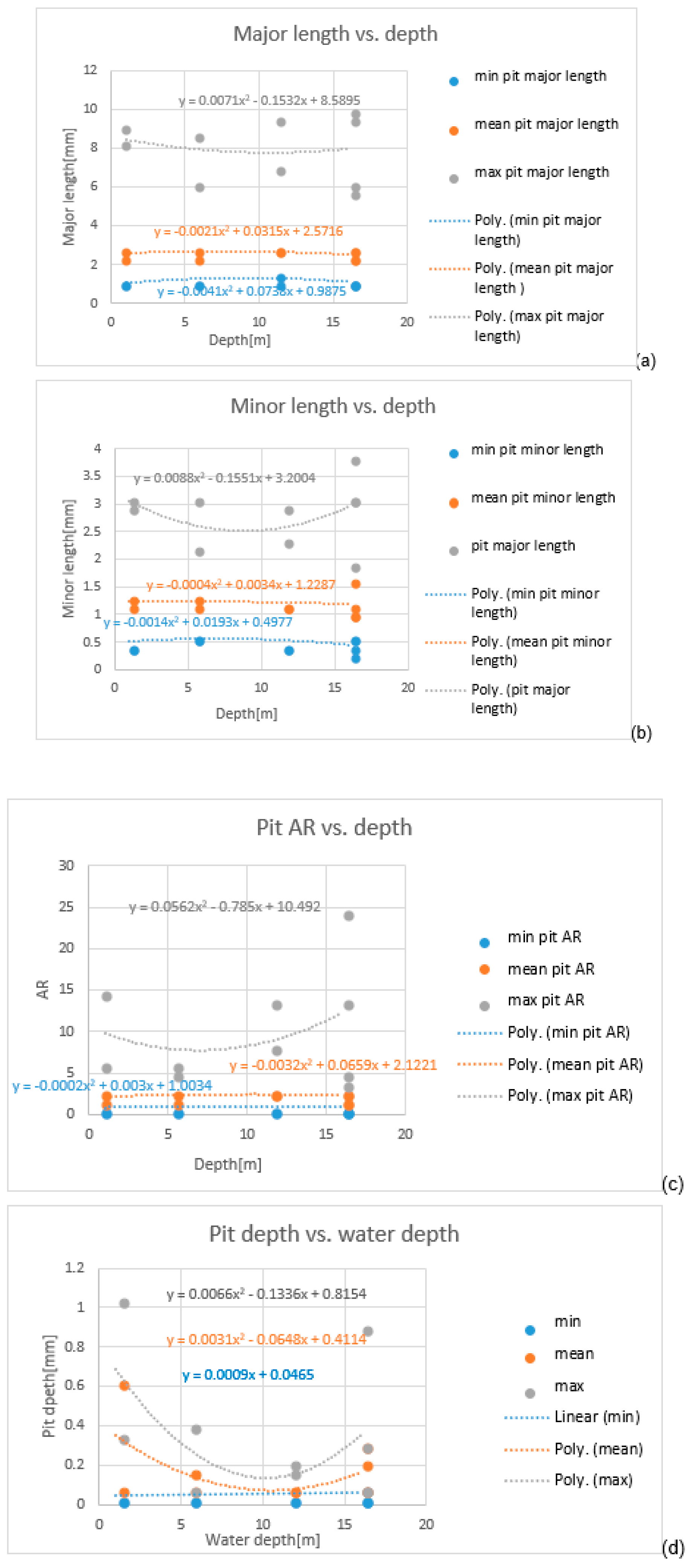
Within the literature, there is a major absence of details on pitting corrosion for steel S355 to water depth; in the authors’ opinion, this is the first time such an exercise has been performed to catalogue those variations, not only for that grade of steel but also for any other material. The extracted features/characteristics of the pits were defined as follows:

• The pit depth;
• The pit major length;
• The pit minor length;
• The aspect ratio;
• The area;
• The number of pits.

For each of the above features, the minimum, maximum, and mean of the pits from each plate were extracted and plotted with the water depth of the deployed coupons.

Owing to its stochastic nature, the most appropriate statistical distribution was fitted to each of the above pit characteristics from each side of the coupons.

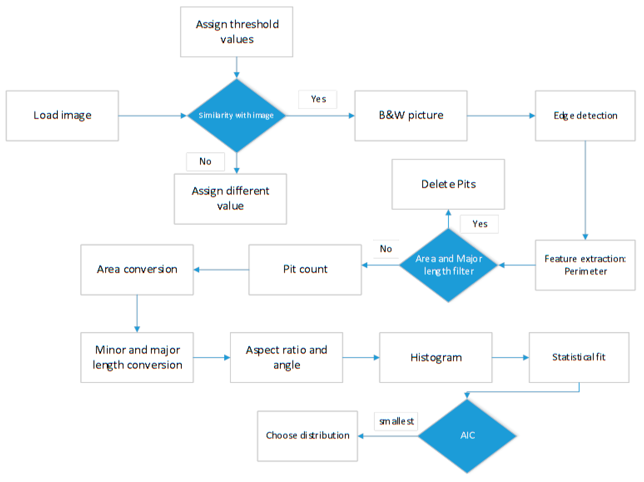
Some noise was detected, and the area and major length were employed to filter this out by applying a threshold of acceptance and rejection based on those dimensional quantities. To make this process fruitful, the following steps were employed, as summarized in the flowchart in Figure 1:

To capture the depth, a mechanical pit gauge was employed to measure at least 20% of the total pits on the surface. The statistical distribution and variation with depth were then determined to characterize the pits on each side of the plates.

Such an exercise is beneficial in making both designers and offshore wind operators aware of the variations caused by pitting corrosion and use realistic values to design against this.

2. Methodology

To assess the coupon using image processing, frottage was employed to replicate the surface of the coupon onto a paper without the effect of the curvature. The nature of this curvature arose during the field experiment and not from manufacturing. The process of frottage was important as this enabled the measured pixels to be converted effectively to metric length when it is known that the length of the coupon is 400 mm.

Once the shading was completed, the drawing was digitalized using a high-resolution scanner. The image was scanned in a grayscale format at the highest resolution available. Unwanted white sections of the paper were digitally trimmed out which would be used as the input for the algorithm.

The first step of the algorithm was the conversion of a grayscale image to a black and white one. This conversion is known as thresholding, denoted in this study by the letter T where a user-defined grey value was set to define the white and black regions, respectively. The logic for the thresholding was as follows:

• When the value of T is less than the threshold value, the binarizing process turns to zero, otherwise it is one.

Following this step, the pit was extracted. To do so, the process of edge detection was applied whereby a closed region of zero was examined to define a pit. Once the pit was obtained, the features characterizing the pit could be extracted.

2.1. Area

The first features extracted were the area, which was simply a count of pixels inside each of the pits multiplied by the area of each pixel. The conversion was defined by the area scale factor. The mathematical expressions are as follows:

$$A={\displaystyle \sum }_{n=1}^n{P}_n$$

(1)

where A is the total pixel area, P is the pixel area, and n is the number of pixels for one pit.

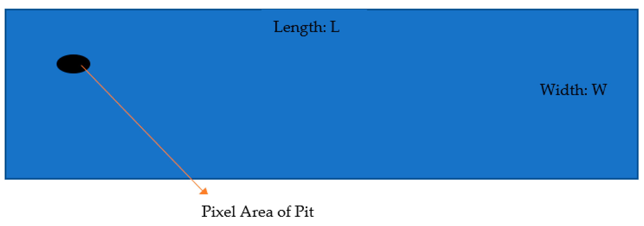
The area scale factor was dependent on the length and width of the plate or coupon and was crucial in changing the units from pixel² to mm². The procedure below explains how this was conducted, with Figure 2 presenting a schematic of the coupon.

The geometrical area of the plate was:

$$A=Area=Length\times Width$$

(2)

$$PA=Pixel Area=P_l\times P_w$$

(3)

where PA is the pixel area of the whole plate determined from the pixel size of the image for the length and width.

$$\frac{A}{PA}=K$$

(4)

where K is the area scale factor.

The actual area of the feature was calculated as:

$$Area of feature \left[{\mathrm{mm}}^2\right]=K\times pixel area of feature$$

(5)

2.2. Minor and Major Length and Aspect Ratio

The minor and major length of the zero clusters were then extracted.

For each feature that was selected, the minor and major lengths were characterized. The major length was simply the longest distance of the pit, and the minor length, the shortest perpendicular distance from that major length. The distance at this current stage was measured in pixels. The orientation was also extracted from the algorithm, which was the angle of the major axis to the x-axis (horizontal) as part of the regionprops function in the image processing toolbox of MATLAB. (2020). version(R2020a). Natick, Massachusetts: The MathWorks Inc. [17].

The length scale factor (LSF) had to be measured in the two axes, where P_x was the pixel length in the x-axis and P_y was the pixel length in the y-axis (vertical):

$$\frac{L}{P_x}=LSFx$$

(6)

$$\frac{W}{P_y}=LSFy$$

(7)

The length L_x and L_y represent the corrected major lengths and were calculated as follows:

$$L_x=Major Length\times LSFx\times \cos \left(\theta \right)$$

(8)

$$L_y=Major Length\times LSFx\times \sin \left(\theta \right)$$

(9)

The same procedure was performed for the minor length extracted, except that the angle θ was corrected by adding it to 90 degrees.

The actual minor and major length in millimeters were calculated using the Pythagorean theorem:

$$Major or Minor length=\sqrt{L_x^2+W_y^2}$$

(10)

The aspect ratio is much simpler as it is dimensionless, and this was determined using the following equation:

$$Aspect Ratio=major length/minor length$$

(11)

2.3. Filtering

The process of filtering was fundamental in removing all the unnecessary noise from the picture. Rather than undergoing an elaborate filtering process, the area and major length were sufficient to remove the unwanted points. The criteria of acceptance were:

• If a pit with a length of fewer than 20 pixels and more than 2 pixels was captured as the major length, this was deleted from the collection of pits.
• If the area was larger than 30 pixel², the pits were deleted.

2.3.1. Pit Depth

The pit gauge was used to measure the depth of the pit. To extract this information using manual labor is time-consuming. For each pit, only 20% of the depth was measured in a random manner for which a minimum, mean, and maximum were found.

The pit gauge had a resolution of 0.05 mm.

2.3.2. Statistical Fit

For the area, aspect ratio, angle, and major and minor length, the most appropriate statistical fit was chosen from a list of the following statistical distributions from MATLAB. These were evaluated against the Akaike Information Criterion (AIC) to determine which fit was the most representative [18]. As a reminder, the AIC assesses the bias versus the precision of the fit. More parameters represent a higher bias and are penalized accordingly:

$$AIC=-2lo{g}_e\left(L\right)+2q$$

(12)

The likelihood L was calculated as:

$$L={\displaystyle \prod }_{i=1}^{n}f\left(x_i\right)$$

(13)

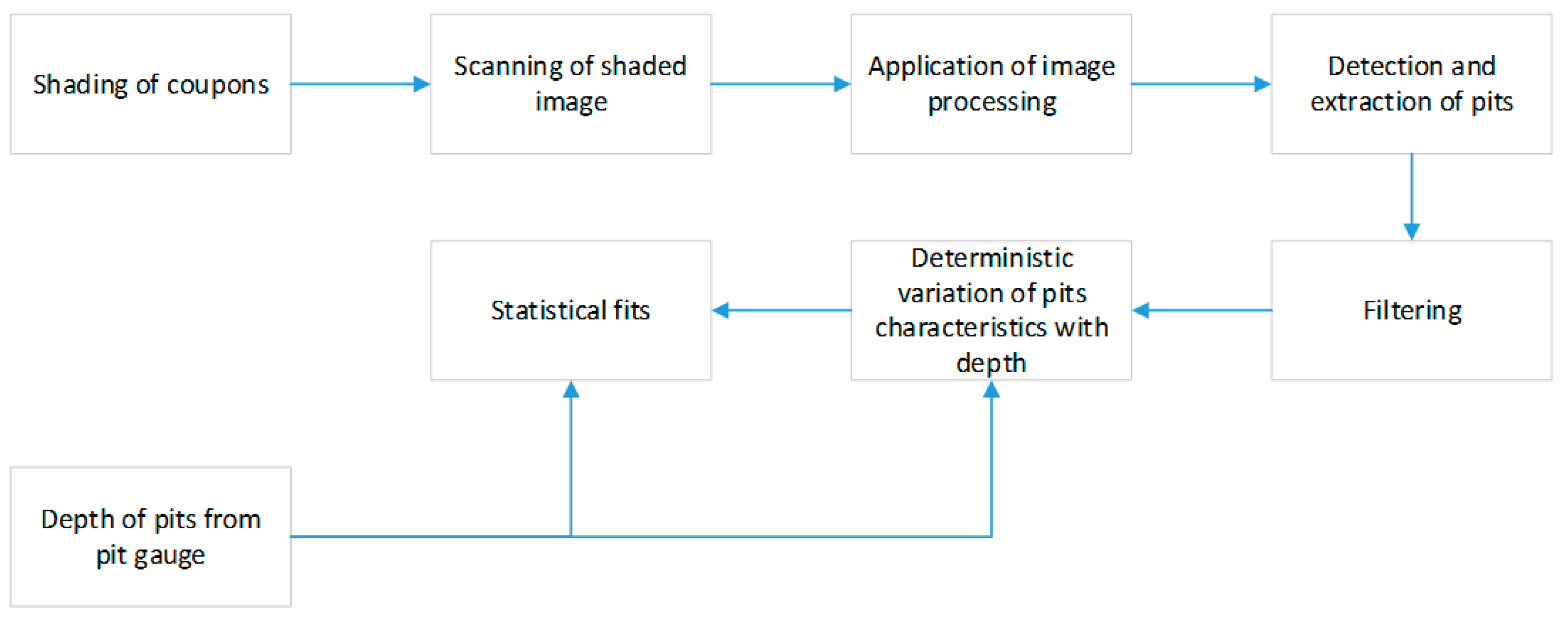
The following flowchart (Figure 3) summarizes the various steps involved:

3. Results

3.1. Number of Pits

This section may be divided by subheadings. It should provide a concise and precise description of the experimental results, their interpretation, as well as the experimental conclusions that can be drawn.

The number of pits detected are presented in

Table 1. Pit data.

Coupon	Probability of Pitting	Number of Pits	Pit Intensity (Pit/m2)	Depth from Seabed (m)
1 Blue back	0.18	124	3.44 × 103	16
1 Blue front	0.23	180	5.00 × 103	16
1 Black back	0.36	285	7.92 × 103	16
1 Black front	0.59	537	1.49 × 104	16
2 Blue back	0.66	240	6.67 × 103	11.5
2 Blue front	0.054	17	4.72 × 102	11.5
3 Black back	0.67	315	8.75 × 103	5.5
3 Black front	0.63	23	6.39 × 102	5.5
4 Blue back	0.54	363	1.01 × 104	1
4 Blue front	0.069	373	1.04 × 104	1

, which also displays the probability of pitting and pit intensity.

The pit intensity was calculated as:

$$\mathrm{pit} \mathrm{intensity}=\frac{\mathrm{number} \mathrm{of} \mathrm{pits}}{\mathrm{Area} \left[{\mathrm{m}}^2\right]}$$

(14)

3.2. Pit Major and Minor Length and Pit Depth

The minor and major lengths are important characteristics of the pit. They must be extracted and have not been given sufficient attention in the literature. In the context of a stress analysis, the pit characteristics are fundamental. The profiling of the pit is performed in terms of the minimum, mean, and maximum length of the pit for each side of the plate.

A fit was therefore applied to mathematically define the profiling to depth for each of the quantities in Figure 4.

4. Discussion

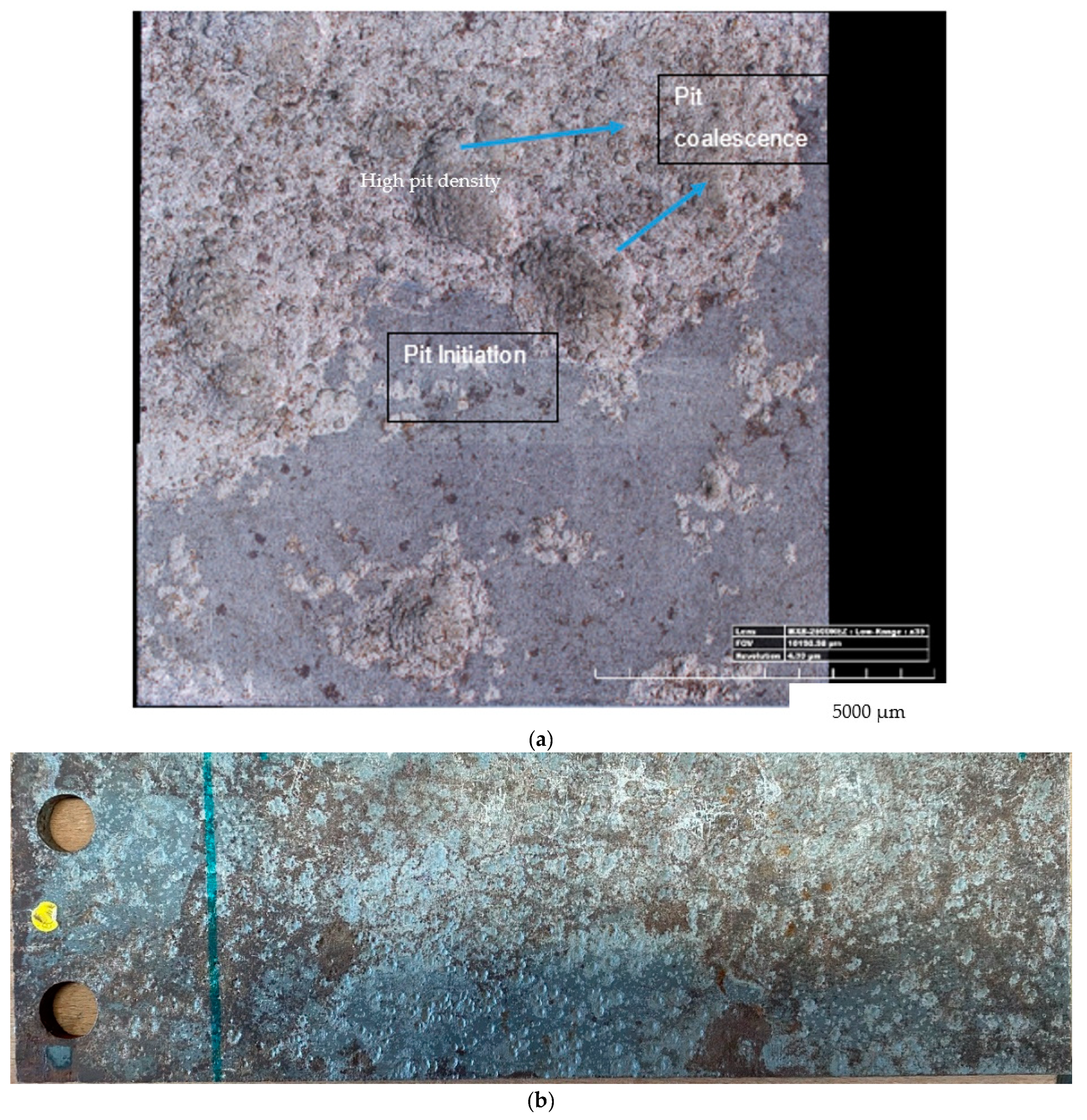
4.1. Visual Inspection of Pits

There were several pits, some in the development stage and others at a micro-level. The image in Figure 5a depicts the pits at different stages of development under an optical microscope along with variations on the same plate but in different areas. A high level of pit density was observed in some plates, as indicated in Figure 5b.

4.2. Pit Detection and Counting

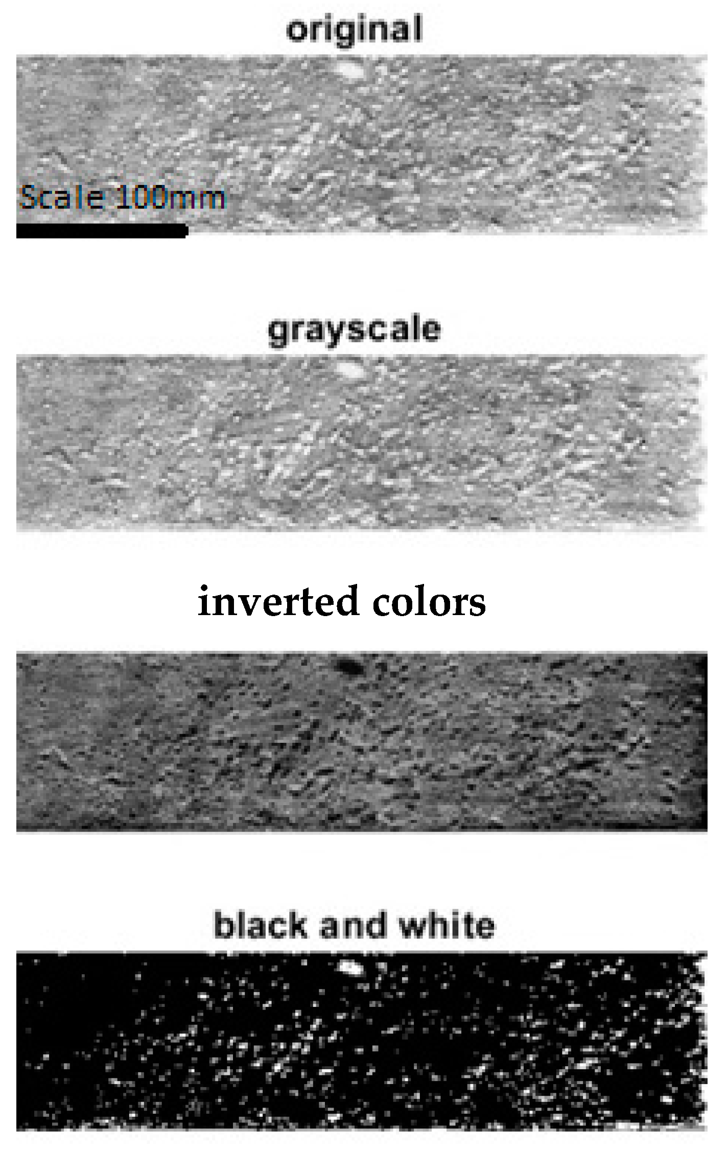
The coupons were all shaded and the surficial conversion of one coupon is depicted in Figure 6. The original image on the diagram illustrates the shaded and scanned coupon. It was then transformed into grayscale to remove the color dimensions of the image. This was inverted for easier viewing of the pits and ultimately binarized through the thresholding process. The images were scanned to a ratio of 1:1.

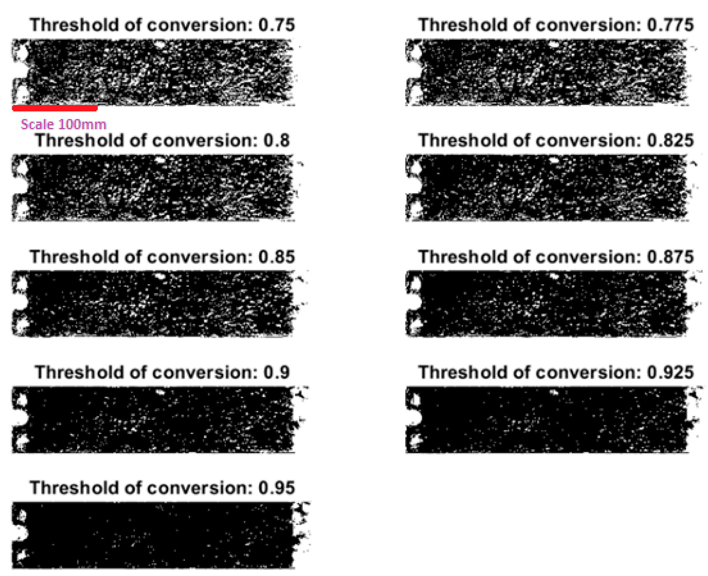
In this case, the pits were from a basic visual inspection. The image processing algorithm was used to extract information about the pits but before doing so, the image had to be re-characterized as a black and white one. The threshold levels also had to be adjusted and compared from a value of 0.75 to 0.95 in steps of 0.025. The comparison was based on the pit count resulting from the algorithm and the pit counts were carried out manually. The black and white image indicates the sensitivity of the thresholding effect on the feature extracted. It is important to note that the thresholding is highly dependent on the conditions of the shading and scanning. The former was conducted by the same person with the same darkness of pencil lead to ensure consistency in the images.

The other aspect that had to be performed, once the white regions had been identified, was to extract the features and count the number of objects. At this stage, despite the thresholding, there was a high level of noise that had to be removed.

The regionprops function in MATLAB. (2020). version(R2020a). Natick, Massachusetts: The MathWorks Inc. was used to extract the potential pits.

The features were then extracted and converted. The smaller pits reached a size of 0.1 mm, which corresponded to the size of 1 pixel. To refine this further, a higher spec scanner could be used, in which case the dimensional representation of the pits can be significantly improved (more pixels to represent 1 mm) but that would add potentially more noise and processing time as the matrix dimension would increase significantly. The filtering allowed the smaller pixels to be removed and the number of pits obtained were tabulated as presented in

Table 2. Number of pits counted.

	Number of Pits Counted
Count 1	498
Count 2	462
Count 3	514
Average	491

.

Following filtration, the maximum number of pits obtained was 537 and the minimum number was 17.

Three individuals counted the pits, and this was used as a benchmark to calibrate the thresholding value for the binarizing process.

The number of pits counted three times and then averaged are presented in Table 2:

The closest to the average indicated in Table 2 is 545.

Table 3. Number of pits calibrated.

Threshold	Number of Pits	% Error
0.75	1216	142.55319
0.775	928	85.106383
0.8	884	76.329787
0.825	695	38.630319
0.85	623	24.268617
0.875	545	8.7101064
0.9	407	−18.81649
0.925	203	−59.50798
0.95	75	−85.03989

presents the error due to the thresholding.

It is extremely difficult to fully understand the reason for this variation. The differences in the number of pits are twofold and were explored as:

• between the same plates but different sides (front and back), and
• between the plates at different depths (total number of pits per plate).

4.2.1. Part (1)

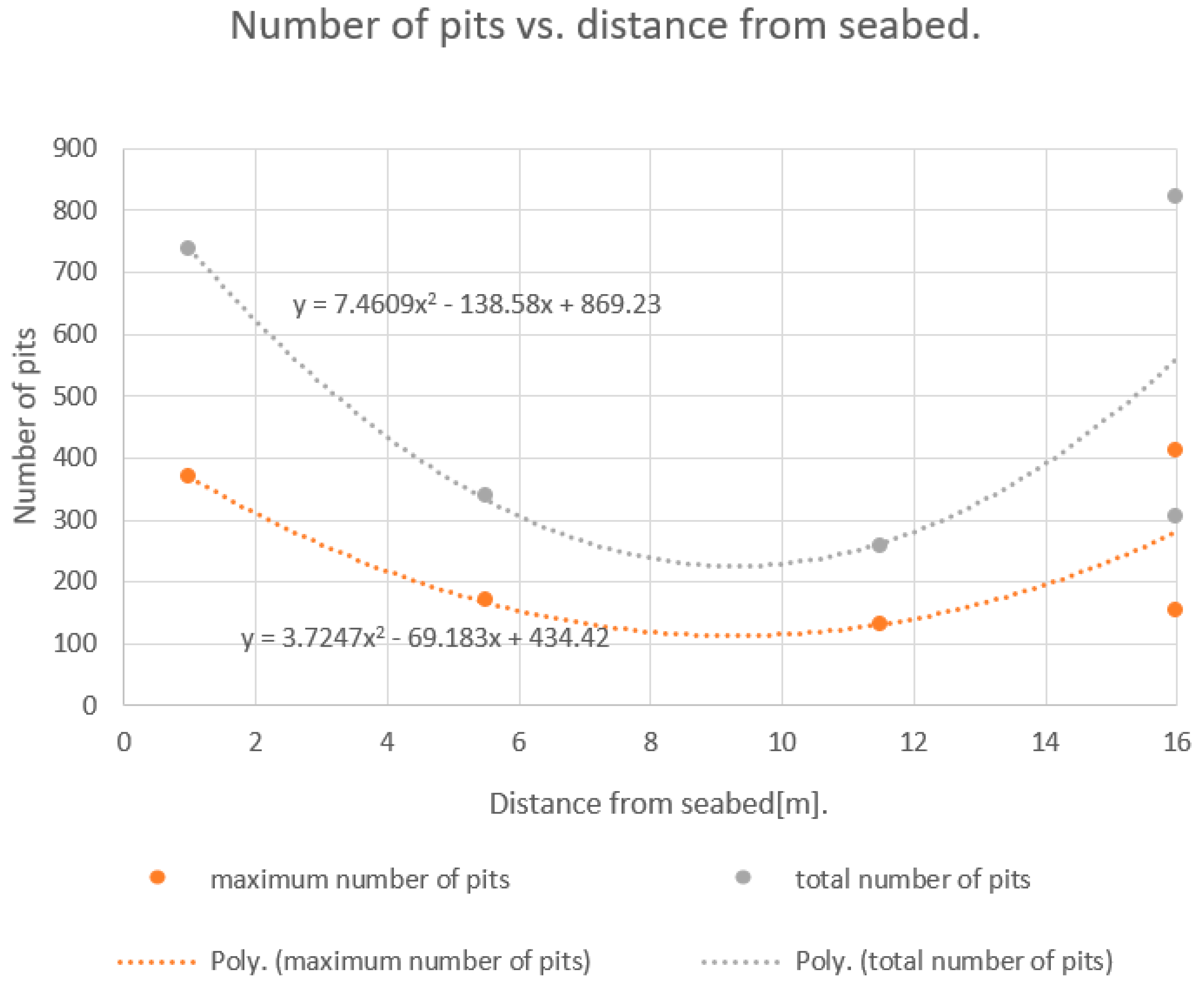
Two aspects of the number of pits were considered for analysis to depth, namely the maximum number of pits for each coupon when compared between sides and finally, the sum of two sides from the same coupon, as presented in Figure 7.

As indicated, the pitting pattern to depth follows a quadratic curve shown in Figure 8. This is counter to the accepted belief that with depth, there is less oxygen and ultimately, less corrosion. This trend demonstrates the complex nature of pitting corrosion and supports the notion that with depth there are fewer pits [3]. This graph indicates that inspection strategies for pitting corrosion must be vigilant at both tidal regions and also seabed regions, especially seabed regions where bending stresses are larger.

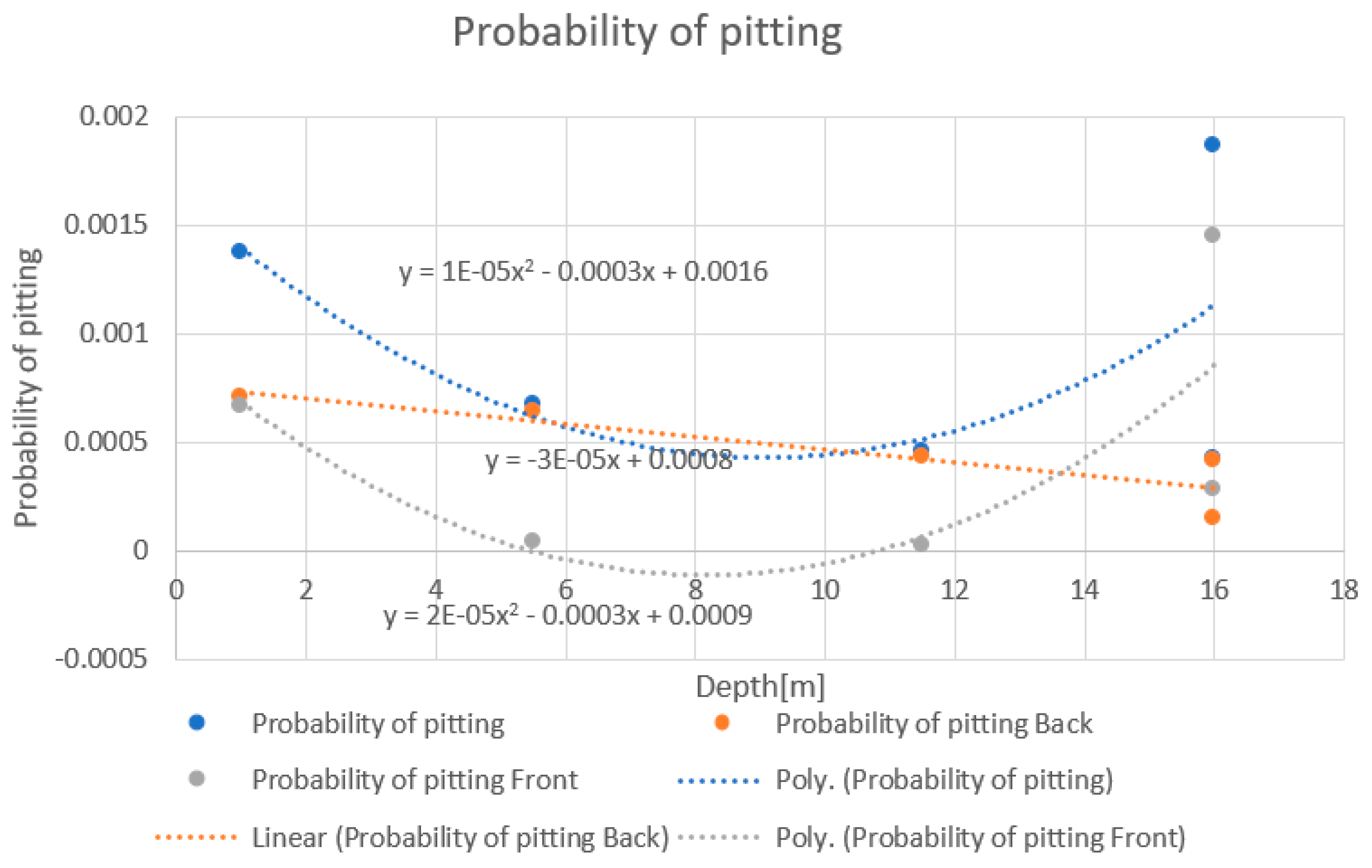
An alternative perspective is to consider the difference between the front and back pitting difference, which is derived from the probability of pitting presented in Figure 9. The probability of pitting is simply the ratio of the total area of pits to the total area of the surface. In this analysis, there are three curves indicating:

• The total area of pits that consider both sides of the coupon, namely the surface area of one side of the coupon is multiplied by two.
• The front coupon indicates the probability of pitting for the front marked surface.
• The back coupon indicates the probability of pitting for the back marked surface.

Despite having pits in the front, this method indicates that between 5.8 and 11.5 m in depth, the number of pits becomes negative. This shows that there are limitations to profiling, which could be averted by deploying more coupons to cover those depths. Chlorine ions are known to be fundamental in the pitting corrosion process. Pitting corrosion is an auto-catalytic process whereby the chlorine ions ensure that the pitting potential is maintained and therefore, progression from initiation, propagation and growth [3]. It is instructive to note that the difference between front and back close to the seabed is negligible. This is where the high nitrogen content of rust and higher levels of sulfur are found. The corrosion attack in terms of pitting corrosion is equally bad. Further away, there is an increasing difference in the number of pits. Here, the levels of oxygen in the Energy Dispersive X-ray Spectroscopy (EDS) results are higher and that of sulfur is lower. This is a clear illustration that the sulfur, which might be a manifestation of Sulphate Reducing Bacteria (SRB), is more prominent and that nitrogen, which enhances marine growth, has a major impact on the chemistry of corrosion but that influence is confined to the seabed area. Oxygen becomes more dominant below the tidal region; therefore, aerobic corrosion is fundamentally more present and the pits initiated are richer in the area where the oxygen levels are higher.

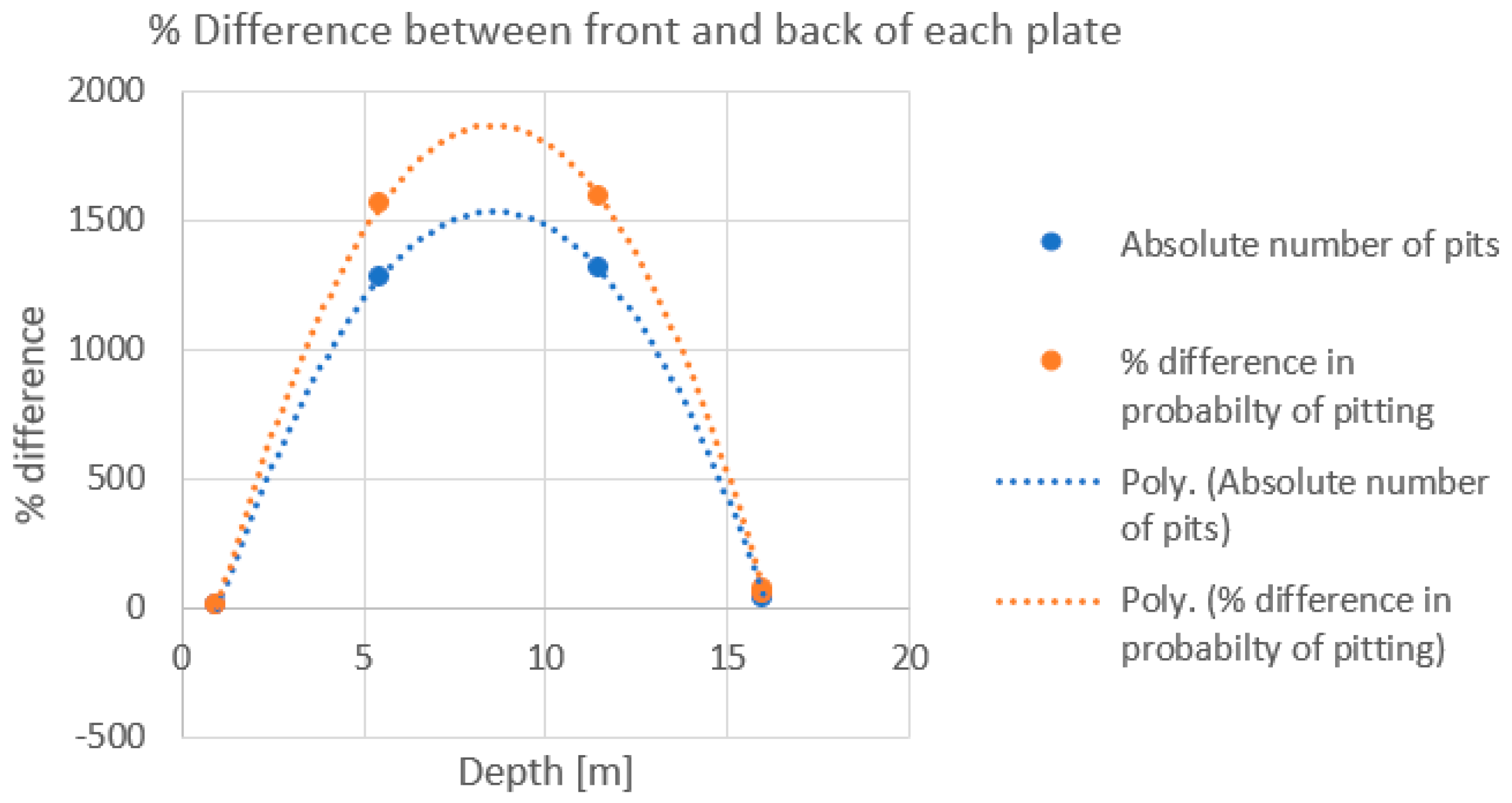
A substantial difference was observed between the back and front of each plate and is plotted in Figure 10. This was quantified in two ways, namely the probability of pitting and the absolute number of pits. In both cases, the variations followed the same trend, but the values were different. The reason for this cannot be fully explained and further monitoring is required to provide a more informed explanation.

4.2.2. Part (2)

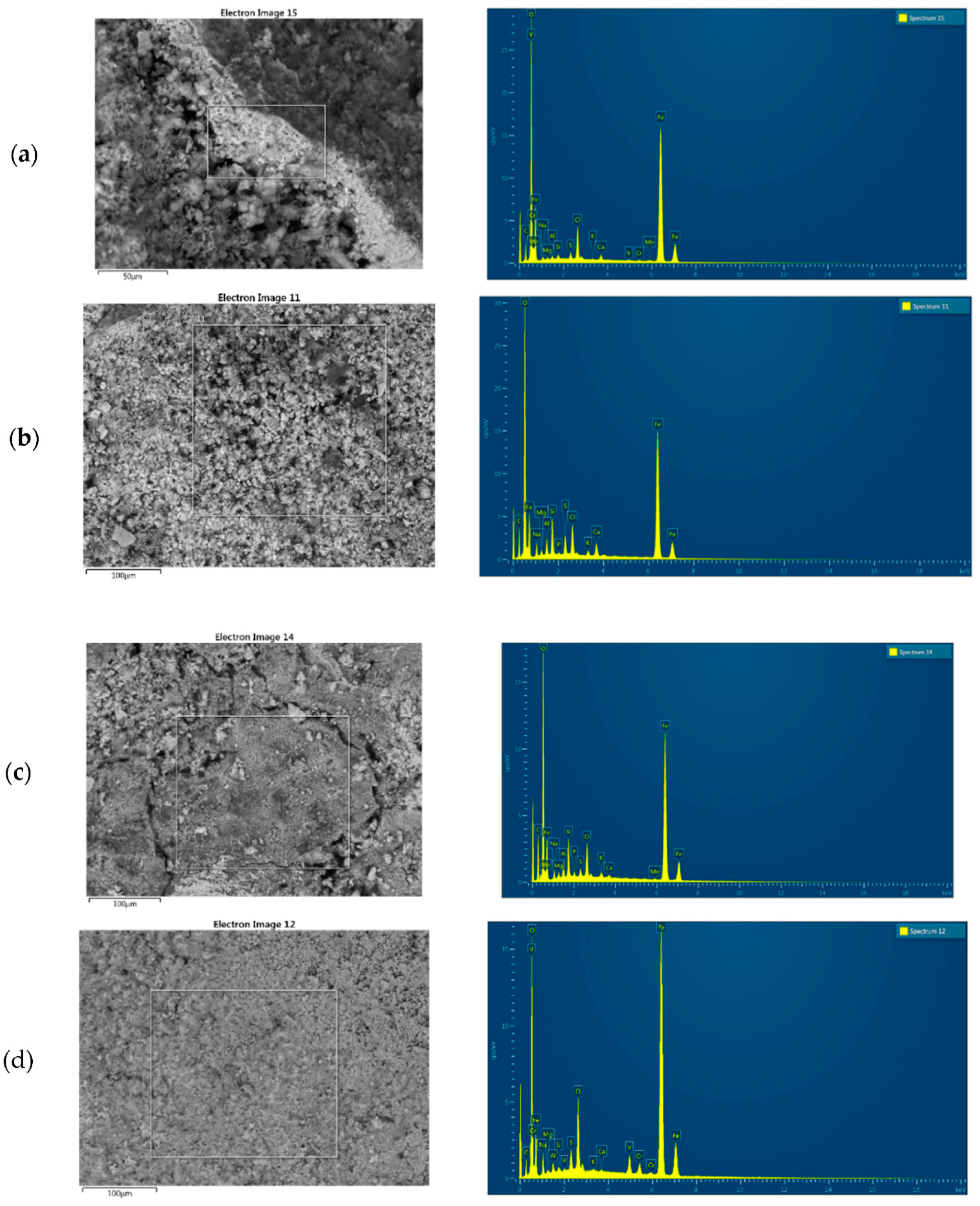
One hypothesis is that close to the sea surface, the levels of oxygen are richer, and this oxygen-rich environment helps to incubate more pits than those exposed at deeper levels. That said, the problem is not simply related to oxygen; it also concerns the chemical composition of the water and the biological content present in the marine ecosystem. The seabed is teeming with life and biological corrosion will have a greater chance of occurring. When the rust sample was subjected to EDS analysis (refer to

Table A1. EDS table percentage weight of elements.

2 Blue
Statistics	N	Na	Mg	Al	Si	P	S	Cl	K	Ca	Ti	V	Cr	Mn	Fe
Max	0	2.54	0.44	1.22	2.34	0.28	1.33	4.21	0.43	1.2	0	2.17	1.08	0.54	57.14
Min	0	0.66	0.18	0.24	0.22	0.11	0.45	2.21	0.07	0.07	0	0.11	0.14	0.21	36.55
Average	0	1.4	0.31	0.71	1.09	0	0.79	2.9	0.3	0.46	0	0	0	0	46.86
1 Black
Statistics	N	Na	Mg	Al	Si	P	S	Cl	K	Ca	Ti	V	Cr	Mn	Fe
Max	0	1.39	0.49	0.62	1.12	0	0.57	3.22	0.22	0.32	0	0.28	0.2	0	61.06
Min	0	0.43	0.19	0.3	0.44	0	0.17	0.88	0.07	0.09	0	0.28	0.2	0	40.56
Average	0	0.8	0.33	0.43	0.7	0	0.34	1.86	0.13	0.22	0	0	0	0	52.55
4 Blue
Statistics	N	Na	Mg	Al	Si	P	S	Cl	K	Ca	Ti	V	Cr	Mn	Fe
Max	6.5	2.52	0.81	3.23	5.58	0.63	1.23	3.22	1.08	1.51	0.18	0.67	0.72	0.35	55.83
Min	4.4	1.02	0.12	0.21	0.28	0.06	0.31	1.35	0.07	0.13	0.18	0.15	0.72	0.35	4.58
Average	5.3	1.51	0.52	1.45	2.27	0.21	0.89	2.29	0.55	0.65	0	0	0	0	39.19
3 Black
Statistics	N	Na	Mg	Al	Si	P	S	Cl	K	Ca	Ti	V	Cr	Mn	Fe
Max	0	0.94	0.38	1.63	2.78	0.05	0.66	2.36	0.34	0.23	0.11	0	0	0.5	64.67
Min	0	0.16	0.37	0.1	0.23	0.05	0.25	0.64	0.12	0.07	0.11	0	0	0.5	40.69
Average	0	0.53	0	0.71	1.2	0	0.48	1.6	0.22	0	0	0	0	0	50.34
1 Blue
Statistics	N	Na	Mg	Al	Si	P	S	Cl	K	Ca	Ti	V	Cr	Mn	Fe
Max	0	2.8	1.48	4.31	11.29	0.23	2.04	4.26	1.46	3.2	0.33	0	0.93	0.41	67.36
Min	0	0.54	0.26	0.49	0.46	0.04	0.31	1.34	0.19	2.34	0.33	0	0.28	0.41	14.3
Average	0	1.3	0	1.75	4.77	0	1.09	2.53	0.68	0	0	0	0	0	38.67

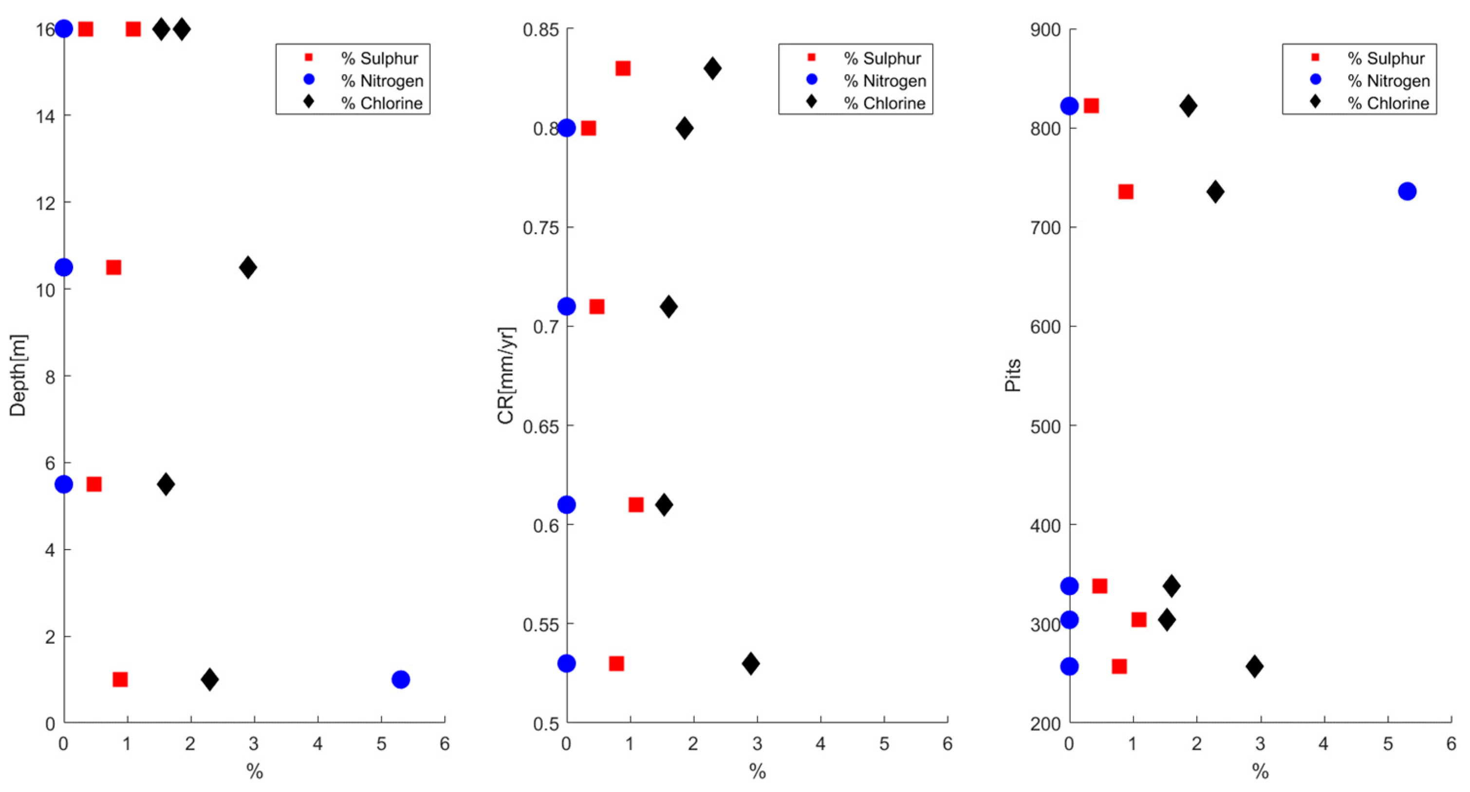
in Appendix A and Figure 11), nitrogen content was found only at the bottom plate, and is an element known to enhance marine fouling. The presence of sulfur is also highly indicative of biological activities. Two other elements must be considered to obtain a better picture of the pitting pattern being observed: chlorine and sulfur. An environment where pitting corrosion thrives must have chlorine as this allows the corrosion current to remain within the pitting range. As indicated in the literature, the higher the percentage composition of chlorine, the higher the pitting corrosion current, which reflects the pitting corrosion rate. Thus, the more pits that are detected, the higher the chlorine levels. The data indicates otherwise and demonstrates that the interacting chemicals in the rust tell a different story.

Figure 11 and Figure 12 indicate that chlorine has a major influence but becomes more pronounced between 1.6 and 2.6%. This seems to disprove the idea that more chlorine means there is more pitting corrosion, which holds true in a controlled environment but not a marine one. The sulfur follows a quadratic format, with a maximum at 16 and 1 m. In terms of corrosion rate, this is highly influenced by the chlorine and follows a trend similar to that of the corrosion rate with depth. The corrosion rate is also strongly influenced by the presence of nitrogen which causes it to increase drastically. Regarding the number of pits, these increase with chlorine content except for the lowest point. The coupon with the rust containing nitrogen is the second highest. This is due to the pits being larger and the presence of pit coalescence. It is an extremely complex analysis as the corrosion takes place in an environment that has a chemical, biological, and physical interaction, each of which is influenced by multiple actors that are dynamic at every single level. Those interactions have to be understood to determine those factors that influence pitting corrosion.

However, at this stage aforementioned, only a partial picture is available; further monitoring of the dynamics of the water quality of the oceans is required to provide additional details. Another explanation might relate to the microstructure of the coupons. Even though the plates are manufactured from the same batch, there may be potential variabilities in their microstructure, which will tend to increase the number of pits. This is a tedious process and will require an elaborate microstructural analysis before and after the coupon is deployed.

4.2.3. Pits’ Characteristics of Statistical Distributions

The plates used to determine the most appropriate statistical fit were those with the most pits at each height. Although it might prove to be rather conservative, the difference is so substantial that it is more optimal to adopt a conservative philosophy rather than a more relaxed one on pitting corrosion.

The best fit for each of them, along with the parameters describing the most appropriate distributions assessed by the AIC, are given in

Table 4. Major length statistical fit.

	Major Length
Coupon	Distribution	Distribution Name			Distribution Values
1 blue back	‘GeneralizedExtremeValue’	‘µ’	‘σ’	‘K’	0.19	0.48	1.89
1 blue front	‘GeneralizedExtremeValue’	‘µ’	‘σ’	‘K’	0.46	0.68	1.96
1 black back	‘GeneralizedExtremeValue’	‘µ’	‘σ’	‘K’	0.16	0.46	1.84
1 black front	‘GeneralizedExtremeValue’	‘µ’	‘σ’	‘K’	0.22	0.73	2.20
2 blue back	‘GeneralizedExtremeValue’	‘µ’	‘σ’	‘K’	0.34	0.68	1.99
2 blue front	‘GeneralizedExtremeValue’	‘µ’	‘σ’	‘K’	0.40	0.51	2.17
3 black back	‘GeneralizedExtremeValue’	‘µ’	‘σ’	‘K’	0.25	0.72	2.03
3 black front	‘lognormal’	‘µ’	‘σ’	‘N/A’	0.88	0.36	0.00
4 blue back	‘GeneralizedExtremeValue’	‘µ’	‘σ’	‘K’	0.25	0.62	1.97
4 blue front	‘GeneralizedExtremeValue’	‘µ’	‘σ	‘K’	0.36	0.69	2.02

,

Table 5. Minor length statistical fit.

	Minor Length
Coupon	Distribution	Distribution Name			Distribution Values
1 blue back	‘lognormal’	‘µ’	‘σ’	‘N/A’	0.01	0.25	0.00
1 blue front	‘lognormal’	‘µ’	‘σ’	‘N/A’	−0.10	0.31	0.00
1 black back	‘GeneralizedExtremeValue’	‘µ’	‘σ’	‘K’	0.08	0.27	1.04
1 black front	‘gamma’	‘a’	‘b’	‘N/A’	7.84	0.20	0.00
2 blue back	‘GeneralizedExtremeValue’	‘µ’	‘σ’	‘K’	0.09	0.30	1.02
2 blue front	‘rayleigh’	‘A’	‘B’	‘N/A’	0.89	0.00	0.00
3 black back	‘lognormal’	‘µ’	‘σ’	‘N/A’	0.21	0.34	0.00
3 black front	‘lognormal’	‘µ’	‘σ’	‘N/A’	0.13	0.31	0.00
4 blue back	‘lognormal’	‘µ’	‘σ’	‘N/A’	0.19	0.33	0.00
4 blue front	‘GeneralizedExtremeValue’	‘µ’	‘σ’	‘K’	0.13	0.28	0.97

and

Table 6. AR statistical fit.

	Aspect Ratio
Coupon	Distribution	Distribution Name			Distribution Values
1 blue back	‘lognormal’	‘µ’	‘σ’	‘N/A’	0.76	0.35	0.00
1 blue front	‘GeneralizedExtremeValue’	‘µ’	‘σ’	‘K’	0.34	0.96	2.18
1 black back	‘GeneralizedExtremeValue’	‘µ’	‘σ’	‘K’	0.06	0.41	1.60
1 black front	‘GeneralizedExtremeValue’	‘µ’	‘σ’	‘K’	0.33	0.37	1.50
2 blue back	‘GeneralizedExtremeValue’	‘µ’	‘σ’	‘K’	0.23	0.58	1.76
2 blue front	‘GeneralizedExtremeValue’	‘µ’	‘σ’	‘K’	0.66	0.80	1.70
3 black back	‘GeneralizedExtremeValue’	‘µ’	‘σ’	‘K’	0.19	0.51	1.69
3 black front	‘lognormal’	‘µ’	‘σ’	‘N/A’	0.74	0.39	0.00
4 blue back	‘GeneralizedExtremeValue’	‘µ’	‘σ’	‘K’	0.27	0.49	1.63
4 blue front	‘GeneralizedExtremeValue’	‘µ’	‘σ	‘K’	0.29	0.63	1.86

.

4.2.4. Pit Depth

Approximately 20% of the total number of pits were randomly measured using a pit gauge. They were then tabulated and the data presented in a histogram for best statistical fit evaluations.

The results for each of the selected coupons are presented in

Table 7. Pit depth statistical fit.

		Pit Depth
Coupon	Distribution	Distribution Name			Distribution Values
1 blue back	‘ExtremeValue’	‘µ’	‘σ’	‘N/A’	0.2441442	0.0471388	0
1 blue front	‘GeneralizedExtremeValue’	‘µ’	‘σ’	‘K’	2.6787865	1.56 × 10−09	0.05
1 black back	‘GeneralizedExtremeValue’	‘µ’	‘σ’	‘K’	3.594312	8.12 × 10−05	0.050022
1 black front	‘rayleigh’	‘A’	‘σ’	‘N/A’	0.2427394	0	0
2 blue back	‘Nakagami’	‘µ’	‘σ’	‘N/A’	1.9877973	0.0092857	0
2 blue front	‘GeneralizedExtremeValue’	‘µ’	‘σ’	‘K’	3.335662	1.68 × 10−05	0.050005
3 black back	‘ExtremeValue’	‘µ’	‘σ’	‘N/A’	0.7111769	0.1776861	0
3 black front	‘GeneralizedExtremeValue’	‘µ’	‘σ’	‘K’	0.4137141	0.030785	0.061047
4 blue back	‘rayleigh’	‘A’	‘B’	‘N/A’	0.1516998	0	0
4 blue front	‘GeneralizedExtremeValue’	‘µ’	‘σ’	‘K’	3.1221115	1.25 × 10−09	0.05

.

The maximum pit depth was 1.05 mm on the coupon closest to the seabed.

The MATLAB. (2020). version(R2020a). Natick, Massachusetts: The MathWorks Inc. image processing toolbox provides the necessary tools for this type of image processing. The processes of image segmentation are included as a function for thresholding and edge detection, which can ultimately be used for feature extraction and object counts [16].

5. Conclusions

This study demonstrates the variation of pitting corrosion with respect to depth. Although a trend has been observed, to build more confidence in the results, similar experiments will have to be repeated in different environments. The variation at the deterministic level indicates that pitting corrosion varies in a quadratic manner with all the characteristics of the pits in the immersed region.

The region close to the seabed has a different environment and, despite lower levels of oxygen, the presence of nitrogen in the rust substrate proved to be a factor that determined not only the higher number of pits but also the deepest ones. The 111 days of exposure also indicates that pit coalescence was taking place where several pits were combining to form a new larger pit. Within those larger pits, smaller pits or micro pits were formed, a factor that tends to be excluded in some studies. According to the literature, these micro pits can increase the SCF by a factor of two [19].

The image processing threshold was set to 0.875 to match the counted pits; once this calibration was completed, the characteristics of the pit were extracted using the region- props function in MATLAB. The probability of pitting was found to be high in the area concerned at 0.6. Another method for determining the probability of pitting as a pit count was also identified, with significant differences observed in both methods.

The statistical fits are important, and it is the first time in the pitting literature that this exercise has been carried out for such profiling. There tends to be a bias for the Generalized extreme value distribution for the major length, pit depth, and the aspect ratio, and lognormal for the minor length after using the AIC.

The purpose of this study was to provide meaningful results that can be used for both simulations of pits at a design level but also from an operational and maintenance perspective.

The key findings can be summarized as follows:

• The number of pits follows a quadratic curve in the immersed region with respect to the pit properties.
• The maximum pit depth was found to be 1.05 mm and was closest to the seabed.
• The experiment needs to be repeated in different environments to increase confidence in the model.
• Statistical fits assessed with the AIC can be used to express the variation of the pits.
• Image processing can be applied to extract pit information such as pit area, pit aspect ratio, and pit minor and major lengths.