Article

A Variable Performance Parameters Temperature–Flowrate Scheduling Model for Integrated Energy Systems

1
Key Laboratory of Energy Thermal Conversion and Control of Ministry of Education, School of Energy and Environment, Southeast University, Nanjing 210096, China
2
Nanjing NARI-RELAYS Electric Co., Ltd., Nanjing 211102, China
*
Author to whom correspondence should be addressed.
These authors contributed equally to this work.
Energies 2021, 14(17), 5400; https://doi.org/10.3390/en14175400
Submission received: 8 July 2021 / Revised: 18 August 2021 / Accepted: 24 August 2021 / Published: 30 August 2021
(This article belongs to the Section F: Electrical Engineering)

Abstract

:
Optimal scheduling strategy of integrated energy systems (IES) with combined cooling, heating and power (CCHP) has become increasingly important. In order to make the scheduling strategy fit to the practical implementation, this paper proposes a variable performance parameters temperature–flowrate scheduling model for IES with CCHP. The novel scheduling model is established by taking flowrate and temperature as decision variables directly. In addition, performance parameters are treated as variables rather than constants in the proposed model. Specifically, the efficiencies of the gas turbine and the waste heating boiler are estimated with the partial load factor, and the coefficient of performance (COP) of the electrical chillers and heat pumps are estimated with the partial load factor and outlet water temperature. Then, to deal with the model nonlinearities caused by considering the variability of COPs, the COP-expansion method is developed by adopting a specific representation of the COP and the expansion of the outlet water temperature. Finally, case studies show that the variable performance parameters’ temperature–flowrate scheduling model can account for the variation of performance parameters, especially the impacts of water temperature and the part load factor on the COP. Therefore, the proposed scheduling model can obtain more adequate and feasible operation strategy, thereby suggesting its applicability in engineering practice.

1. Introduction

In recent years, increased global awareness has grown on the comprehensive utilization of multiple energy [1]. The integrated energy systems (IES) with combined cooling, heating, and power (CCHP) [2] can contribute to improve the efficiency of energy production and reduce the emissions; therefore, it has been recognized as a good option for future energy systems [3,4].
A lot of work has been done on the optimal scheduling problem of IES. The common control modes for IES with CCHP are following thermal load (FTL) and following electric load (FEL). Based on FTL and FEL, Fang [5] introduced an integrated performance criterion and then proposed an improved optimal operation strategy in order to balance the energy efficiency and emissions. Wang [6] proposed an FEL-based operation strategy for IES by following the average electric load. However, these control modes take no account of the operational coordination of multiple energy demands and forms. Therefore, different unified optimization scheduling models are proposed.
The typical unified optimization scheduling models used in IES firstly require a structured and comprehensive modeling framework to describe energy conversion devices, in which the conversion efficiencies of devices are described by many performance parameters. In the process of implementing scheduling strategy, performance parameters such as the coefficient of performance (COP) of the electrical chiller/heat pump and the efficiency of the gas turbine or boiler vary over a wide range for various factors and can generally not reach the rating value [7]. Therefore, the true condition in practice can not accord with the scheduling strategy in optimization scheduling models when taking performance parameters as constants such as the rating value. It is necessary to consider the variation of performance parameters. Moreover, different from the efficiency of the gas turbine or the boiler which is mainly influenced by the partial load factor [8], through the analysis in [9,10], the COP of an ordinary water-cooled chiller is influenced not only by the partial load factor but also the water temperature. Like the increase of the cooling water temperature, there is an increase in the COP, but correspondingly there is also an increase in the pumping power because of larger water flowrate caused by the smaller temperature difference. It is also necessary to consider the impact of water temperature because of the compromise of the pumping power and the high-COP.
Typical unified optimization scheduling models include mixed integer linear programming (MILP) and mixed integer nonlinear programming (MINLP). Taking performance parameters as variables can bring about quadratic cross-product nonlinear terms, and the MILP models are usually established without considering the variability of performance parameters. Performance parameters, such as the efficiency of the boiler and the COP of the chiller, are all simplified into constants. For instance, Li [11] proposed an optimal dispatch strategy for IES with CCHP and wind power, in which the COPs of chillers and the efficiency of the electricity boiler were constants. Arcuri [12] addressed an MILP model to solve the operational strategy of a system equipped with compression and absorption heat pump, based on the simplifying supposition that all the COPs of the pumps stayed constant. Liu [13] presented the long-term optimal planning for an CCHP considering demand response and energy storage, with all the COP (efficiency) of energy conversion technology being supposed as constants. Zeng [14] presented a day-ahead scheduling model for multi-energy interconnected region based on the centralized energy transition framework, in which the efficiencies of the waste heat boiler/gas boiler, and the COPs of chillers/air conditioners were all treated as constants. In addition, performance parameters in the MILP models for a CCHP system with thermal storage tanks [15], community integrated energy systems [16], a microenergy grid [17], and the distributed energy system [18] were all simplified into constants. However, as indicated above, performance parameters for some devices usually change in a large range, and only taking performance parameters as constants is over-simplified and can not accord with the true condition. The MINLP model is another common optimization method, which can consider the nonlinear characteristic of performance parameters and very much accords with the practical process. For instance, Chen [19] presented a superstructure CCHP system and optimization strategies for operations, in which the COPs of chillers were variables and varied with part load ratio. Ma [20] proposed a particle swarm optimization based algorithm for a new distributed energy system integrating cogeneration, photovoltaic, and ground source heat pump, in which all the thermal performance parameters were expressed by quadratic fitting formulas. Lu [21] established an MINLP-based model to get the optimization strategies of building energy systems considering energy generation and storage, taking the impact of multiple factors on COP into account. Some other studies considering variable performance parameters have been reported in the literature (e.g., [22,23,24,25]). However, MINLP has defects of low robustness, slow speed, and complicated computation in solving [26] compared with MILP. Thus, it is not the preferred candidate for the optimization scheduling model in IES.
A few works have considered the variation of thermal performance parameters in the framework of an MILP model. Li [27] established a system-wide coordinated energy optimization model for a hybrid energy microgrid in both the grid-connected and islanded modes. Similarly, Jiang [28] proposed an operation dispatch method based on price response for a multi-energy system integrating micro-CHP and smart appliances. Luo [29] proposed a novel two-stage coordinated control mode for CCHP microgrid energy management. Carrion [30] proposed a computationally efficient MILP model to solve the unit commitment problem of thermal units. In those studies, the thermal and electrical efficiencies of the gas turbine were defined as variables, by introducing piecewise linear function to fit input electric energy and output thermal energy relationship of the gas turbine directly. Because the input energy of the device can represent the partial load, the energy input–output piecewise linear function is equivalent to only consider the impact of partial load factor. However, some performance parameters, like the COPs of chillers or heat pumps, are also influenced by water temperature of devices. The above-mentioned scheduling models were all established only taking the energy transfer of devices as decision variables, and the water temperature was not even a decision variable. Thus, these energy-transfer based scheduling models can not take the impact of water temperature on performance parameters into account. Moreover, some devices such as chillers and heat pumps, can not implement the energy transfer instruction, and the load control of these devices is achieved by controlling the outlet temperature and flowrate indirectly. Thus, the results of energy-transfer based scheduling models can not be directly applied to the control device. Only few researchers have stepped further by introducing constraints of the temperature in a scheduling model. Lv [30] established an optimal operation of heat network and buildings in the form of the temperature and flowrate, and Gu [31] proposed a scheduling model considering the transmission process together with the thermal inertia of buildings with temperature parameters. Wei [32] proposed a temperature–flowrate based scheduling model that directly adopted temperature and flowrate as decision variables. Although the studies above have significant merits, this scheduling model still specified all performance parameters as constants.
The present study is motivated to explore this issue. In contrast to studies mentioned above, this paper proposes a variable performance parameter temperature–flowrate scheduling model for IES. This scheduling model has two-fold merits: (1) The proposed scheduling model takes flowrate and temperature as decision variables which means that the scheduling results can be directly applied to the control device; (2) Performance parameters are treated as variable, more precisely, the efficiencies of the gas turbine and the waste heat boiler are estimated with the partial load factor, and the COPs of the electrical chiller and heat pump are estimated with the partial load factor and outlet water temperature collectively. To deal with the model nonlinearities caused by considering the variability of COPs, a linearization technique called the COP-expansion method is also developed by adopting a specific representation of the COP and the expansion of the outlet water temperature. In addition, case studies are conducted based on the data for a typical day, which suggest their feasibility in practice.
The rest of this paper is organized as follows. In Section 2, the conventional energy–transfer based scheduling modeling process of the IES is present, which is the preparation and groundwork. In Section 3, a variable performance parameters temperature–flowrate scheduling model is established. Section 4 demonstrates the case studies conducted and the discussion based on the data for a typical day. The last section concludes the paper.

2. Preliminaries

In this section, the description of IES is given, and a conventional energy-transfer based scheduling model is established as preparation. The conventional scheduling model takes the energy transfer of devices as decision variables rather than the temperature and the flowrate, and all the performance parameters are treated as fixed values.

2.1. System Description

A typical schematic representation of IES with CCHP is illustrated in Figure 1. Multiple energy demands including cooling, heating, and electricity to end users are supplied simultaneously in the IES. The electrical demand is mainly supplied by the photovoltaic array (PV), wind power (WP), gas turbine (GT), power gird (GD), and battery (BA). IES will purchase insufficient electricity from GD to meet the demand of electricity, and the BA will store excess electricity, so the BA is to shift the surplus electricity at off-peak hours to on-peak hours; For the hot water, there are two carriers: two heat pumps (HP) and a waste heat boiler (WHB). The WHB can recycle the waste energy generated by the GT; meanwhile, HPs can make use of the geothermal energy to produce hot water for end users; An absorption chiller (AC) and two electrical chillers (EC) are used to supply the cooling demand. The EC is driven by the electricity and the AC can recycle the low-grade hot water from the WHB to produce the chilled water. Then, water from the AC and ECs is mixed before being pumped into the cold water network and charged into the water tank (TA) when excessive. In addition, the TA can also discharge cold water to meet the insufficient cooling demand.
With multiple energy carriers and diversified coupling processes, some assumptions and simplifications of the scheduling model are necessary. There is no thermal loss for all heat exchangers in the IES; the calorific value of natural gas is constant; the IES can purchase limited grid electricity but can not sell back to the power grid; and the inlet water temperature of the TA can be well controlled at a constant. The hydraulic energy consumed by water pumps has a linear relationship to the working fluid flowrate. The COP of the AC is taken as fixed value. In addition, the values of system structure and capacity parameters are given in Table 1.

2.2. Energy-Transfer Based Scheduling Model

2.2.1. Electricity Subsystem Modeling

The GT can produce electrical and thermal energy simultaneously, which is an important energy-saving equipment in the IES. Its scheduling model is formulated as:
E G T ( t ) = F G T ( t ) η G T L H V
with the following constraints:
δ G T ( t ) E G T m i n E G T ( t ) δ G T ( t ) E G T m a x μ G T E G T m a x ( t ) E G T ( t ) E G T ( t 1 ) μ G T E G T m a x ( t ) | | δ G T ( t ) = 0 | | δ G T ( t 1 ) = 0 , i f t 1 δ G T o n ( t ) δ G T ( t ) δ G T ( t 1 ) , i f t 1
where E G T ( t ) is the generated electricity (kW) at the time t, F G T ( t ) denotes the volume flowrate of natural gas (m3/h), E G T m a x / E G T m i n are the upper and lower operation boundaries of GT, η G T is the electrical efficiency, LHV is the low latent energy of natural gas (kJ/m3), μ G T is the ramp rate factor, δ G T ( t ) is the start and stop state of the GT, and a bool variable δ G T o n ( t ) is introduced to represent the start-up process of GT, if δ G T ( t ) is 1 and δ G T ( t 1 ) is 0, then δ G T o n ( t ) is 1, else δ G T o n ( t ) will be zero because of the start-up penalty item in the objective function, which will be introduced in Section 3.4.
In this IES, a BA is deployed for peak-shaving. At the beginning and the end of a day, the state of the BA is constrained to be equal to fully utilize its adjustment function. Therefore, the model of BA is described as:
S B A ( t ) = S B A ( t 1 ) + E B A , c h ( t ) η B A , c h Δ t E B A , d i s ( t ) η B A , d i s Δ t i f t 1 S B A ( t ) = S B A s t a r t + E B A , c h ( t ) η B A , c h Δ t E B A , d i s ( t ) η B A , d i s Δ t i f t = 0 S B A m i n S B A ( t ) S B A m a x S B A ( e n d ) = S B A m i n δ B A , c h ( t ) E B A , c h m i n E B A , c h ( t ) δ B A , c h ( t ) E B A , c h m a x δ B A , d i s ( t ) E B A , d i s m i n E B A , d i s ( t ) δ B A , d i s ( t ) E B A , d i s m a x δ B A , c h ( t ) + δ B A , d i s ( t ) 1
where S B A ( t ) is total electricity in the BA (kWh) at the time t, S B A s t a r t is initial electricity in the battery (kWh); E B A , c h ( t ) / E B A , d i s ( t ) are the charge and discharge rates (kW), η B A , c h / η B A , d i s are the charge and discharge efficiencies, δ B A , c h ( t ) / δ B A , d i s ( t ) are the charge and discharge states.
GD works as the compensation and sustentation for the IES. The IES can purchase electricity from GD but can not sell back to the GD:
E G D m i n E G D E G D m a x

2.2.2. Hot Water Subsystem Modeling

The WHB and HP work as hot water suppliers in the IES. The WHB is deployed to recover waste heat of GT to produce steam. The steam generated by WHB is utilized in two ways: supplying the heating load or being injected into the AC to produce cold water. The scheduling model of WHB is formulated as:
H W H B , s t e a m ( t ) = H W H B I N ( t ) η W H B
with the following constraints:
H W H B I N ( t ) = ( F G T ( t ) L H V E G T ( t ) ) η r e c H W H B , h o t ( t ) = H W H B , s t e a m ( t ) H A C I N ( t ) δ W H B ( t ) H W H B m i n H W H B , s t e a m ( t ) δ W H B ( t ) H W H B m a x δ W H B ( t ) = δ G T ( t )
where H W H B I N ( t ) is recovery heat energy from waste heat generated by GT (kWh) at the time t, η r e c is waste heat recovery factor, H W H B , s t e a m ( t ) is steam energy generated by WHB, η W H B is the thermal efficiency of WHB, H W H B , h o t ( t ) / H A C I N ( t ) are energy applied to heating load and injected into the AC (kWh), respectively, δ W H B ( t ) is the start and stop state of the WHB, which is supposed to follow the state of GT.
Since the heat generated by the WHB and electricity generated by the GT are coupled, the operation of WHB is not flexible enough to produce hot water. Due to these operation constraints, two HPs are deployed to replenish the shortage of hot water driven by the geothermal energy. Such ability can also be quantified by the COP. The scheduling models of HPs can be written as:
H H P i ( t ) = E H P I N , i ( t ) C O P H P i
with the following constraints as follows:
δ H P i ( t ) H H P m i n H H P i ( t ) δ H P i ( t ) H H P m a x μ H P H H P m a x H H P i ( t ) H H P i ( t 1 ) μ H P H H P m a x | | δ H P i ( t ) = 0 | | δ H P i ( t 1 ) = 0 , i f t 1 δ H P o n , i ( t ) δ H P i ( t ) δ H P i ( t 1 ) , i f t 1
where H H P i ( t ) is heating energy generated by the i-th HP at the time t (kWh), E H P I N , i ( t ) represents electric energy that the i-th HP consumes (kWh), C O P H P i is the COP of the i-th HP, μ H P is the ramp rate factor, H H P m a x / H H P m i n are the upper and lower operation boundaries, δ H P i ( t ) is the start and stop state of the i-th HP, and δ H P o n , i ( t ) represents the start-up process of the i-th HP. It should be noted that, in this system, the HPs are only used to provide hot water, and not for cold water.

2.2.3. Cold Water Subsystem Modeling

The AC converts the heating energy provided by WHB into cooling energy. In addition, the scheduling model of an AC is expressed as follows:
Q A C ( t ) = H A C I N ( t ) C O P A C
with the following constraints:
δ A C ( t ) Q A C m i n Q A C ( t ) δ A C ( t ) Q A C m a x δ A C o n ( t ) δ A C ( t ) δ A C ( t 1 ) , i f t 1
where Q A C ( t ) is the cooling output of AC (kWh) at the time t, H A C I N ( t ) is heating energy of steam generated by WHB and injected into AC (kWh), C O P A C is the COP of the AC, Q A C m a x / Q A C m i n are the upper and lower operation limits, δ A C ( t ) is the start and stop state of the AC, and δ A C o n ( t ) represents the start-up process of AC.
Different from the AC, the ECs generate cooling energy according to the principle of the reversed Carnot cycle. The scheduling models of ECs are governed by:
Q E C i ( t ) = E E C I N , i ( t ) C O P E C i
with the following constraints:
δ E C i ( t ) Q E C m i n Q E C i ( t ) δ E C i ( t ) Q E C m a x μ E C Q E C m a x Q E C i ( t ) Q E C i ( t 1 ) μ E C Q E C m a x | | δ E C i ( t ) = 0 | | δ E C i ( t 1 ) = 0 , i f t 1 δ E C o n , i ( t ) δ E C i ( t ) δ E C i ( t 1 ) , i f t 1
where Q E C i ( t ) is cooling output generated by the i-th EC at the time t (kWh), E E C I N , i ( t ) represents electric energy that the i-th EC consumes (kWh), C O P E C i is the COP of the i-th EC, μ E C is the ramp rate factor, Q E C m a x / Q E C m i n are the upper and lower operation boundaries, δ E C i ( t ) is the start and stop state of the i-th EC, and δ E C o n , i ( t ) represents the start-up process of the i-th EC.
Considering the policy of peak and valley time price in this system, the water storage tank can reduce the electrical consumption of peak power and adding that of the valley power period. It can effectively reduce the power cost. The excess cold water produced by AC and EC is charged into the TA, or discharged conversely from the TA when necessary. The scheduling model of TA is governed by:
S T A ( t ) = S T A ( t 1 ) + Q T A , c h ( t ) η T A , c h Δ t Q T A , d i s ( t ) η T A , d i s Δ t i f t 1 S T A ( t ) = S T A s t a r t + Q T A , c h ( t ) η T A , c h Δ t Q T A , d i s ( t ) η T A , d i s Δ t i f t = 0 S T A m i n S T A ( t ) S T A m a x S T A ( e n d ) = S T A m i n δ T A , c h ( t ) Q T A , c h m i n Q T A , c h ( t ) δ T A , c h ( t ) Q T A , c h m a x δ T A , d i s ( t ) Q T A , d i s m i n Q T A , d i s ( t ) δ T A , d i s ( t ) Q T A , d i s m a x δ T A , c h ( t ) + δ T A , d i s ( t ) 1
where S T A ( t ) is total cold energy in the TA (kWh), S T A s t a r t is initial electricity in the tank (kWh); Q T A , c h ( t ) / Q T A , d i s ( t ) are the charge/discharge rates (kW), η T A , c h / η T A , d i s are the charge/discharge efficiencies, and δ T A , c h ( t ) / δ T A , d i s ( t ) are the charge/discharge states.

3. Variable Performance Parameters Temperature–Flowrate Model

In the conventional scheduling model of the last section, COPs of EC/HP and efficiency of GT/WHB are simplified as fixed values, which is not according with the true condition in practice. However, if C O P E C i / C O P H P i and η G T / η W H B are treated as variables, the product of performance parameters and input energy are all nonlinear terms, namely E E C I N , i ( t ) C O P E C i , E H P I N , i ( t ) C O P H P i , F G T ( t ) η G T , H W H B I N ( t ) η W H B . COPs of EC/HP( C O P E C i / C O P H P i ) change much more with not only the partial load factor, but also the outlet water temperature of EC/HP. With consideration of the problems above, a variable performance parameters temperature–flowrate scheduling model for IES is proposed in this section, which directly adopts temperature and flowrate as decision variables and performance parameters such as C O P E C i / C O P H P i and η G T / η W H B are all variables; especially, the COP-expansion method is proposed to deal with the model nonlinearities when considering the variability of COP.

3.1. Variable Efficiencies of GT/WHB

Taking η G T as an example, it mainly changes with the load rate of GT. It means that η G T is a function of the load E G T ( t ) . Considering E G T corresponds directly to the input volume flowrate of gas ( F G T ), and η G T is also a function of F G T ( t ) . By using the regression method to fit the distribution of the real data, η G T is estimated with the F G T as follows:
η G T = f 1 ( F G T ) = a G T F G T 2 + b G T F G T + c G T
where a G T , b G T , and c G T 
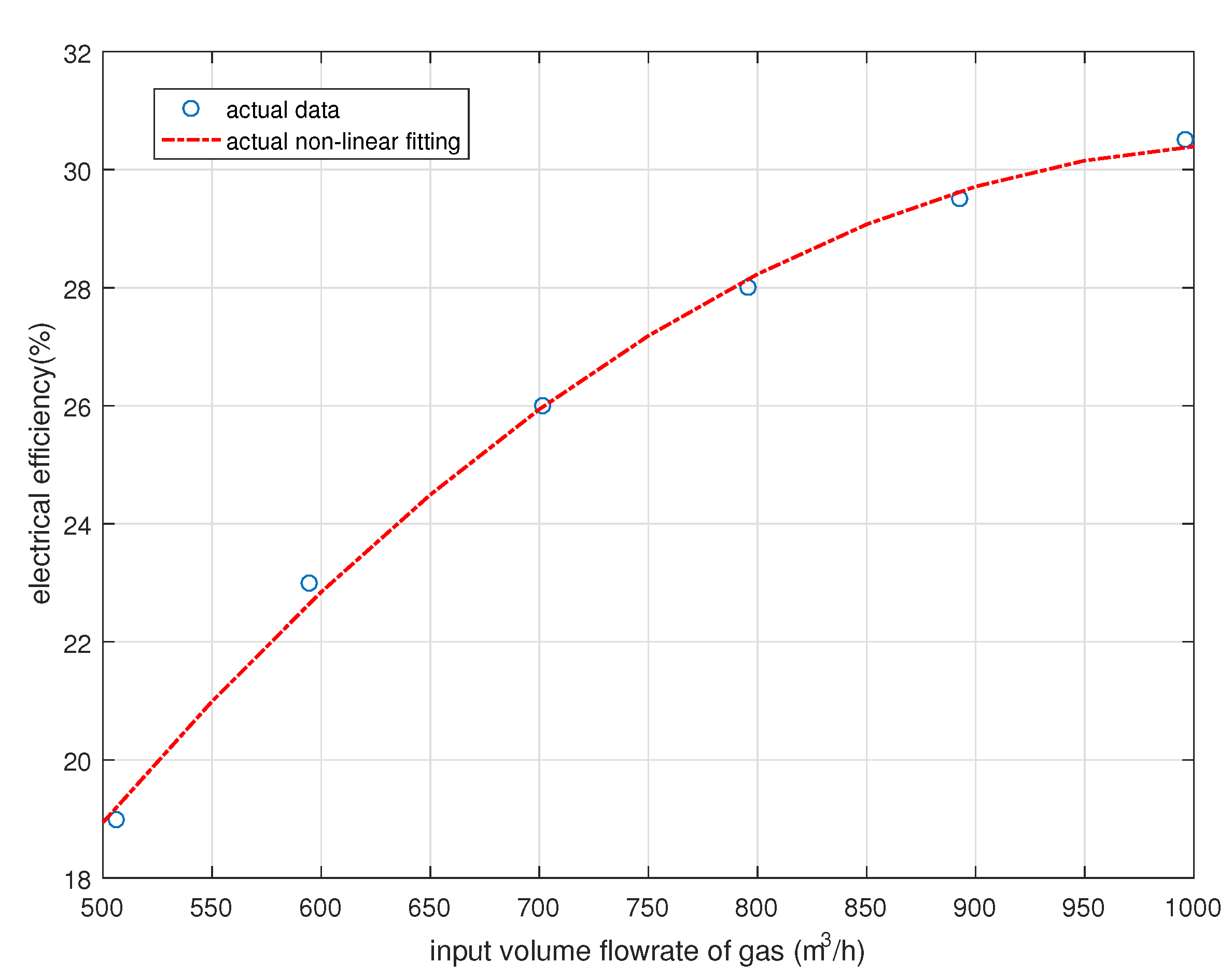
are the regression coefficients. The efficiency curve of GT is shown in Figure 2, in which the scatter data points are on-the-spot operating data from IES in China, and the curve is fitted by the on-the-spot investigation. In this case, Equation (1) can be expressed as:
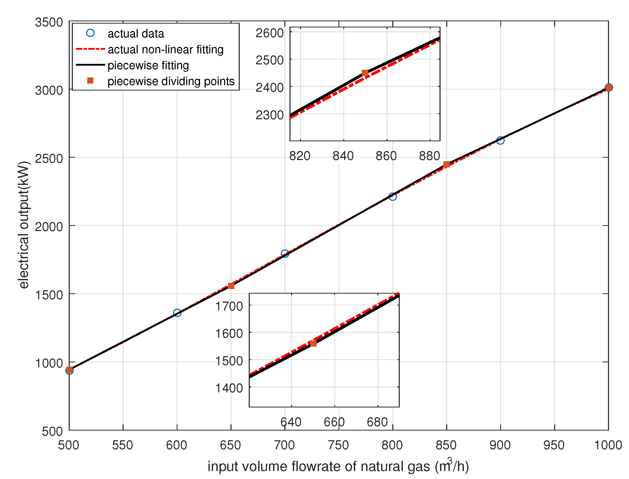
E G T ( t ) = F G T ( t ) f 1 ( F G T ( t ) ) L H V = f 2 ( F G T ( t ) )
Therefore, E G T ( t ) is a nonlinear function f 2 of F G T ( t ) . In order to transform the nonlinear optimal problem into a linear one, there is a three-segment piecewise linear function to approach nonparametric transformation f 2 .
Then, Equation (15) can be converted as:
E G T ( t ) = p i e c e w i s e [ ( x G T 1 , x G T 2 ) , ( k G T 1 , k G T 2 , k G T 3 ) , ( x G T 0 , y G T 0 ) ] ( F G T ( t ) )
where p i e c e w i s e [ ( x G T 1 , x G T 2 ) , ( k G T 1 , k G T 2 , k G T 3 ) , ( x G T 0 , y G T 0 ) ] represents a three-segment piecewise linear function as shown in Figure 3, the first array ( x G T 1 , x G T 2 ) specifies the x-coordinate of the two breakpoints and the second array ( k G T 1 , k G T 2 , k G T 3 ) specifies the slopes of the three segments, the geometric coordinates of at least one point of the function, ( x G T 0 , y G T 0 ) must also be specified. In this way, the nonlinear model of GT can be transformed to linear one.
As for WHB, in the same way, η W H B is estimated with the H W H B I N as follows:
η W H B = a W H B H W H B I N 2 + b W H B H W H B I N + c W H B
where a W H B , b W H B , and c W H B are the regression coefficients. Similarly, a three-segment piecewise linear function can be used to linearize Equation (5), and then we can get
H W H B , s t e a m ( t ) = p i e c e w i s e [ ( x W H B 1 , x W H B 2 ) , ( k W H B 1 , k W H B 2 , k W H B 3 ) , ( x W H B 0 , y W H B 0 ) ] ( H W H B I N ( t ) )
Unlike the E G T ( t ) , H W H B ( t ) can not directly be applied to control the devices. Thus, the outlet temperature of hot water is firstly linearly approximated by 2 K points in its domain [ T W H B , o u t m i n , T W H B , o u t m a x ] , and K is the interval number, namely
T W H B , o u t ( t ) = T W H B , o u t m i n + Δ T W H B k = 1 K 2 k 1 z W H B , k ( t ) Δ T W H B = T W H B , o u t m a x T W H B , o u t m i n 2 K
T W H B , i n ( t ) , T W H B , o u t ( t ) are the inlet and outlet temperature of hot water. Then, the binary expansion method is applied to decompose H W H B ( t ) into the temperature and the flowrate as follows:
c p [ q W H B ( t ) T W H B , o u t m i n + Δ T W H B k = 1 K 2 k 1 v W H B , k ( t ) ] = q W H B ( t ) c p T W H B , i n ( t ) + H W H B , h o t ( t ) 0 q W H B ( t ) v W H B , k ( t ) q W H B m a x [ 1 z W H B , k ( t ) ] k 0 v W H B , k ( t ) q W H B m a x z W H B , k ( t ) k q W H B ( t ) q W H B m a x δ W H B ( t ) z W H B , k ( t ) δ W H B ( t ) k
in which q W H B ( t ) is the hot water flowrate(kg/s) at the time t. z W H B , k ( t ) is the binary variable and v W H B , k ( t ) is an auxiliary variable which can be interpreted as the equivalent flow of the k-th temperature range, Δ T W H B is the outlet temperature resolution, k = 1 , 2 , . . . , K . In addition, it is also necessary to model the auxiliary water pumps for individual devices. For simplicity, it is assumed that the hydraulic energy consumed by water pumps E p u m p , W H B ( t ) essentially has a linear relationship to the working fluid flowrate, thus q W H B ( t ) as expressed below:
E p u m p , W H B ( t ) = q W H B ( t ) E p u m p , W H B m a x / q W H B m a x
By using Equations (18) and (20), all the nonlinear terms are transferred into linear ones, which can be solved efficiently by some commercial solvers.

3.2. Variable COPs: The COP-Expansion Method

Different from η G T / η W H B which is mainly influenced by only one factor, namely the partial load factor, the COPs of EC/HP are influenced not only by the load rate but also the outlet temperature of EC/HP. Therefore, a COP-expansion is proposed to handle COPs of EC/HP.
Taking the COP of the EC ( C O P E C i ) as an example, firstly, the model of EC should directly take temperature and flowrate as decision variables in order to reflect the impact of outlet temperature setpoint on the COP. Similarly to WHB, the outlet water temperature of EC is linearly approximated by 2 K as follows:
T E C , o u t i ( t ) = T E C , o u t m i n + Δ T E C k = 1 K 2 k 1 z E C , k i ( t ) Δ T E C = T E C , o u t m a x T E C , o u t m i n 2 K
Then, the cooling output generated by the i-th EC Q E C i ( t ) is supposed to be decomposed into the temperature and the flowrate as follows:
c p [ q E C i ( t ) T E C , o u t m i n + Δ T E C k = 1 K 2 k 1 v E C , k i ( t ) ] = q E C i ( t ) c p T E C , i n ( t ) + Q E C i ( t ) 0 q E C i ( t ) v E C , k i ( t ) q E C m a x [ 1 z E C , k i ( t ) ] k 0 v E C , k i ( t ) q E C m a x z E C , k i ( t ) k q E C i ( t ) q E C m a x δ E C i ( t ) z E C , k i ( t ) δ E C i ( t ) k
where c p is the specific heat capacity of water, and q E C i ( t ) is the i-th EC cold water flowrate(kg/s) at the time t. T E C , i n ( t ) is the inlet temperature of all the EC, which equates to the return temperature of cold water, and T E C , o u t i ( t ) is the outlet temperature of the i-th EC, T E C , o u t i ( t ) is linearly approximated by 2 K points in its domain [ T E C , o u t m i n , T E C , o u t m a x ] , Δ T E C is the outlet temperature resolution, z E C , k i ( t ) is the binary variable, and v E C , k i ( t ) is an equivalent flow auxiliary variable.
C O P E C i 
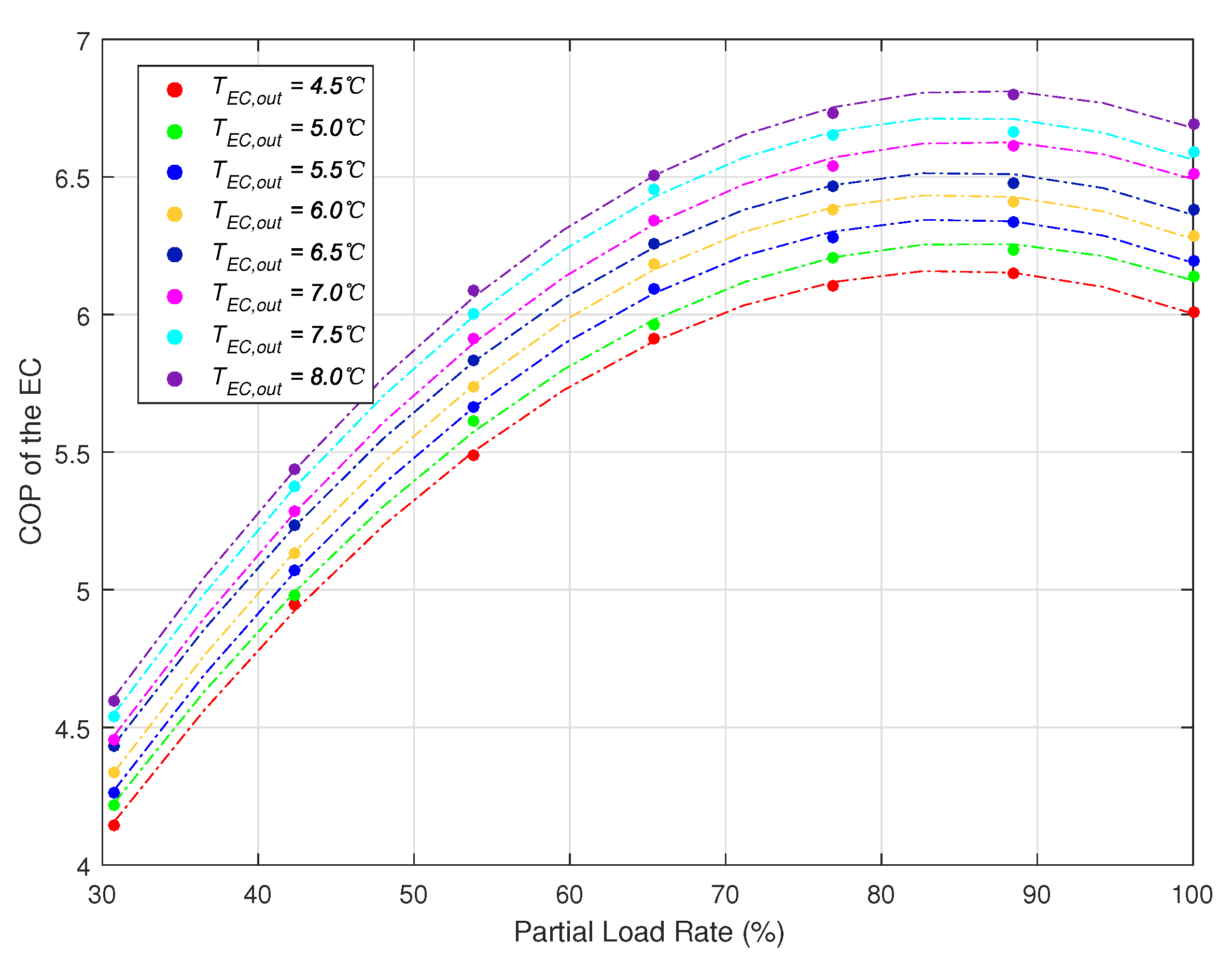
is greatly influenced by the partial load rate and the outlet temperature. Figure 4 shows the partial load rate on the COP of the EC under different outlet temperatures, in which the scatter data points are the actual operating sample data of chillers in IES in China, and the curves of COP under different outlet temperatures are fitted by the samples at the corresponding temperature. The COP increases with an increase in the outlet temperature of EC. Additionally, under different fixed T E C , o u t i , the COP shows the same trends, that is, it firstly increases and then decreases with the increase of the partial load rate. According to this, the influence of the part load factor and the outlet temperature on C O P E C i are independent. Based on this simplified assumption, C O P E C i = f 1 ( E E C I N , i ) · g 1 ( T E C , o u t i ) , where E E C I N , i is the input electric energy, which can represent part load factor. Furthermore, g ( T E C , o u t i ) can be assumed as a linear function because the C O P E C i is less affected by T E C , o u t i . Thus, C O P E C i can be fitted as the following form:
C O P E C i = f 2 ( E E C I N , i ) · [ 1 + α E C ( T E C , o u t i ( t ) T E C , o u t m i n ) ]
where f 2 ( E E C I N , i ) = f 1 ( E E C I N , i ) · g 1 ( T E C , o u t m i n ) represents the partial load transform function when the outlet temperature is set as T E C , o u t m i n , and α E C is a discount coefficient of COP. Equation (24) indicates that, under any partial load, each degree increase of the outlet temperature leads to COP of the EC increases by α E C . Then, Q E C i ( t ) can be expressed as:
Q E C i ( t ) = E E C I N , i ( t ) · C O P E C i ( t ) = E E C I N , i ( t ) · f 2 ( E E C I N , i ( t ) ) · [ 1 + α E C ( T E C , o u t i ( t ) T E C , o u t m i n ) ] = f ( E E C I N , i ( t ) ) + α E C · f ( E E C I N , i ( t ) ) ( T E C , o u t i ( t ) T E C , o u t m i n ) = f ( E E C I N , i ( t ) ) + α E C · f ( E E C I N , i ( t ) ) Δ T E C k = 1 K 2 k 1 z E C , k i ( t )
where f ( E E C I N , i ( t ) = E E C I N , i ( t ) · f 2 ( E E C I N , i ( t ) ) is a nonlinear function that can be approached by a piecewise linear one. The final form of Q E C i ( t ) only contains product terms of the continuous variable and the binary variable, which can be linearized by introducing some auxiliary variables as follows:
Q E C , b a s e i ( t ) = f ( E E C I N , i ( t ) ) w E C , k i ( t ) = Q E C , b a s e i ( t ) z E C , k i ( t )
Substituting Equation (26) into Equation (25), we can obtain that
Q E C , b a s e i ( t ) = p i e c e w i s e [ ( x E C 1 , x E C 2 ) , ( k E C 1 , k E C 2 , k E C 3 ) , ( x E C 0 , y E C 0 ) ] E E C I N , i ( t ) ) Q E C i ( t ) = Q E C , b a s e i ( t ) + α E C Δ T E C k = 1 K 2 k 1 w E C , k i ( t ) w E C , k i ( t ) z E C , k i ( t ) Q E C m a x k 0 Q E C , b a s e i ( t ) w E C , k i ( t ) [ 1 z E C , k i ( t ) ] Q E C m a x k
Equation (27) makes out that, if the outlet temperature is set as T E C , o u t m i n , the i-th EC generates cooling output Q E C , b a s e i ( t ) when it consumes E E C I N , i ( t ) electric energy. In addition, if the outlet temperature setpoint increases to T E C , o u t i ( t ) , the temperature difference between inlet and outlet decreases and flowrate increases, the COP of the EC increases by α E C ( T E C , o u t i ( t ) T E C , o u t m i n ) , with the result that the cooling output of the i-th EC increases from Q E C , b a s e i ( t ) to Q E C i ( t ) under the same power input E E C I N , i ( t ) . 
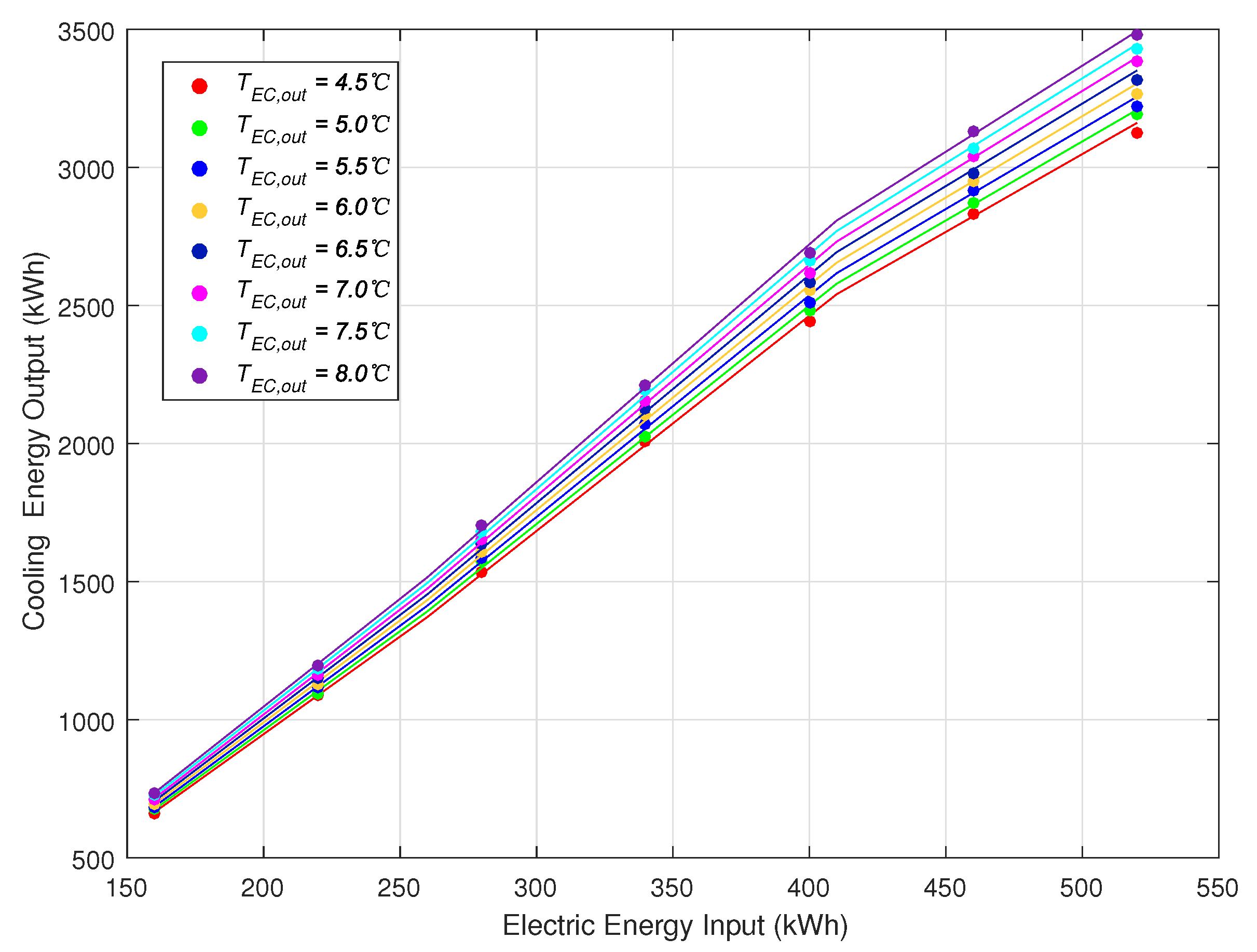
Figure 5 is a diagram of cooling output and electric energy input calculated by Equation (27), the cooling output Q E C i ( t ) fits the sample data well, and our method gets a good compromise between modeling precision and linearization complexity.
By using Equations (23) and (27), all the nonlinear terms have been linearized. The energy consumed by water pumps E p u m p , E C ( t ) is expressed as:
E p u m p , E C i ( t ) = q E C i ( t ) E p u m p , E C m a x / q E C m a x
A similar model of HP can also be obtained by this method. The outlet water temperature of HP is linearly approximated by 2 K as follows:
T H P , o u t i ( t ) = T H P , o u t m i n + Δ T H P k = 1 K 2 k 1 z H P , k i ( t ) Δ T H P = T H P , o u t m a x T H P , o u t m i n 2 K
Then, the thermal energy output generated by the i-th HP H H P i ( t ) is supposed to be decomposed as follows:
c p [ q H P i ( t ) T H P , o u t m i n + Δ T H P k = 1 K 2 k 1 v H P , k i ( t ) ] = q H P i ( t ) c p T H P , i n ( t ) + H H P i ( t ) 0 q H P i ( t ) v H P , k i ( t ) q H P m a x [ 1 z H P , k i ( t ) ] k 0 v H P , k i ( t ) q H P m a x z H P , k i ( t ) k q H P i ( t ) q H P m a x δ H P i ( t ) z H P , k i ( t ) δ H P i ( t ) k
where q H P i ( t ) is the i-th HP hot water flowrate(kg/s) at the time t. T H P , i n ( t ) is the inlet temperature of all the HP, which equates to the return temperature of hot water, and T H P , o u t i ( t ) is the outlet temperature of the i-th HP, T H P , o u t i ( t ) is linearly approximated by 2 K points in its domain [ T H P , o u t m i n , T H P , o u t m a x ] , Δ T H P is the outlet temperature resolution, z H P , k i ( t ) is the binary variable, and v H P , k i ( t ) is an equivalent flow auxiliary variable. By the same method, we can obtain the linearized form of HP’s output:
H H P , b a s e i ( t ) = p i e c e w i s e [ ( x H P 1 , x H P 2 ) , ( k H P 1 , k H P 2 , k H P 3 ) , ( x H P 0 , y H P 0 ) ] E H P I N , i ( t ) H H P i ( t ) = H H P , b a s e i ( t ) α H P Δ T H P k = 1 K w H P , k i ( t ) 2 k 1 w H P , k i ( t ) z H P , k i ( t ) H H P m a x k 0 H H P , b a s e i ( t ) w H P , k i ( t ) [ 1 z H P , k i ( t ) ] H H P m a x k
The energy consumed by water pumps E p u m p , H P ( t ) is expressed as:
E p u m p , H P i ( t ) = q H P i ( t ) E p u m p , H P m a x / q H P m a x

3.3. Linearization for Flow and Energy Balance

The hot water generated by the WHB and HPs is mixed before being delivered to the hot water network, leading to the fluid flow balance as:
q H ( t ) = q W H B ( t ) + i = 1 n H P q H P i ( t )
and energy balance as:
c p [ q W H B ( t ) T W H B , o u t ( t ) + i = 1 n H P q H P i ( t ) T H P , o u t i ( t ) ] = q H ( t ) c p T H ( t )
where T H ( t ) is the hot water network temperature, n H P is the amount of HP, and q H ( t ) is the water mass flowrate (kg/s). This equation containing the product of the fluid temperature and flowrate is nonlinear, so the binary expansion method is applied again to linearize such equation. Assume the temperature of supply hot water T H ( t ) can only vary within certain ranges [ T H m i n , T H m a x ] and linearly approximated by 2 K points, namely:
T H ( t ) = T H m i n + Δ T H k = 1 K 2 k 1 z H , k ( t ) Δ T H = T H m a x T H m i n 2 K
Then, the fluid flow and energy balance equation of hot water in Equation (34) can be rewritten as the following constraints:
0.5 q H ( t ) Δ T H q W H B ( t ) T W H B m i n + Δ T W H B k = 1 K 2 k 1 v W H B , k ( t ) + i = 1 n H P { q H P i ( t ) T H P m i n + Δ T H P k = 1 K 2 k 1 v H P , k i ( t ) } q H ( t ) T H m i n Δ T H k = 1 K 2 k 1 v H , k ( t ) 0.5 q H ( t ) Δ T H v H , k ( t ) z H , k ( t ) q H m a x k 0 q H ( t ) v H , k ( t ) q H m a x [ 1 z H , k ( t ) ] k
where q W H B ( t ) T W H B m i n + Δ T W H B k = 1 K 2 k 1 v W H B , k ( t ) , for example, is the linearization form of q W H B ( t ) T W H B , o u t ( t ) . Thus, the first equation in Equation (36) is the linearization form of energy balance equation of hot water in Equation (34).
As for cold water, in the cooling charge process, the cold water generated by AC and EC is firstly mixed and then pumped into the cold water network to feed the cooling demand and charged into the TA when excessive. In the cooling discharge process, the outlet water of AC, EC, and TA is mixed and delivered to the cold water network to meet the cooling load demand. The charge/discharge cold water flowrate of TA q T A , c h ( t ) / q T A , d i s ( t ) can be calculated by:
Q T A , c h ( t ) = c p q T A , c h ( t ) ( T r e t , Q T T A ) Q T A , d i s ( t ) = c p q T A , d i s ( t ) ( T r e t , Q T T A )
where T r e t , Q is the return cold water temperature as a known quantity, and T T A is the charge/ discharge cold water temperature of TA also as a known quantity. In the same way, assuming the temperature of supply cold water T Q ( t ) can only vary within certain ranges [ T Q m i n , T Q m a x ] and linearly approximated by 2 K points, namely:
T Q ( t ) = T Q m i n + Δ T Q k = 1 K 2 k 1 z Q , k ( t ) Δ T Q = T Q m a x T Q m i n 2 K
The fluid flow and energy balance equation of cold water can be expressed as the following constraint:
q Q ( t ) + q T A , c h ( t ) = q A C ( t ) + i = 1 n E C q E C i ( t ) + q T A , d i s ( t ) 0.5 q Q ( t ) Δ T Q q A C ( t ) T A C m i n + Δ T A C k = 1 K 2 k 1 v A C , k ( t ) + i = 1 n E C { q E C i ( t ) T E C m i n + Δ T E C k = 1 K 2 k 1 v E C , k i ( t ) } + ( q T A , d i s ( t ) q T A , c h ( t ) ) T T A q Q ( t ) T Q m i n Δ T Q k = 1 K 2 k 1 v Q , k ( t ) 0.5 q Q ( t ) Δ T H v Q , k ( t ) z Q , k ( t ) q Q m a x k 0 q Q ( t ) v Q , k ( t ) q Q m a x [ 1 z Q , k ( t ) ] k
It should be noted that, in the cooling charge process, the temperature of mixed water generated by AC and EC must be stable in order to keep natural stratification of cold water in TA. This means that the model must meet at least one requirement: (1) The TA is in the cooling discharge process; and (2) the temperature of mixed water T Q is stable at T T A :
δ T A , d i s ( t ) = 1 | | T Q m i n + Δ T Q k = 1 K 2 k 1 z Q , k ( t ) = T T A
where | | represents logic 
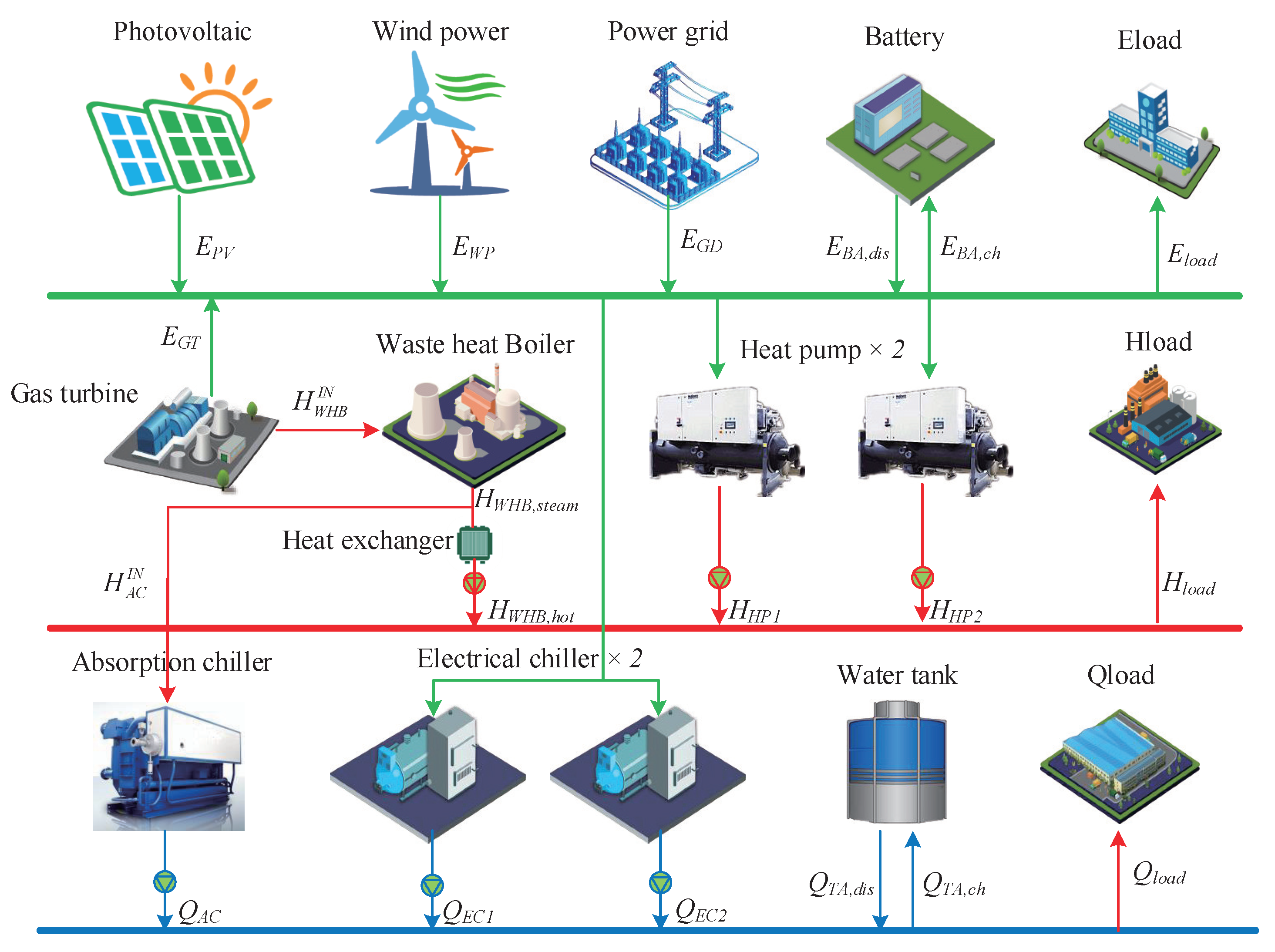
Or. The electricity balance of IES at the time t is expressed as:
E P V ( t ) + E W P ( t ) + E G T ( t ) + E G D ( t ) + E B A , d i s ( t ) = E l o a d ( t ) + E B A , c h ( t ) + i = 1 n E C E E C I N , i ( t ) + i = 1 n H P E H P I N , i ( t ) + E p u m p ( t )
where E p u m p ( t ) represents all the pump power:
E p u m p ( t ) = E p u m p , W H B ( t ) + E p u m p , A C ( t ) + i = 1 n E C E p u m p , E C i ( t ) + i = 1 n H P E p u m p , H P i ( t )
The outlet water of the AC, two ECs and TA are collected to supply the cooling demand, leading to the energy balance of cold water as:
Q A C ( t ) + i = 1 n E C Q E C i ( t ) + Q T A , d i s ( t ) = Q l o a d ( t ) + Q T A , c h ( t )
Similarly, the energy balance of hot water is expressed as:
H W H B ( t ) + i = 1 n H P H H P i ( t ) = H l o a d ( t )

3.4. Optimization

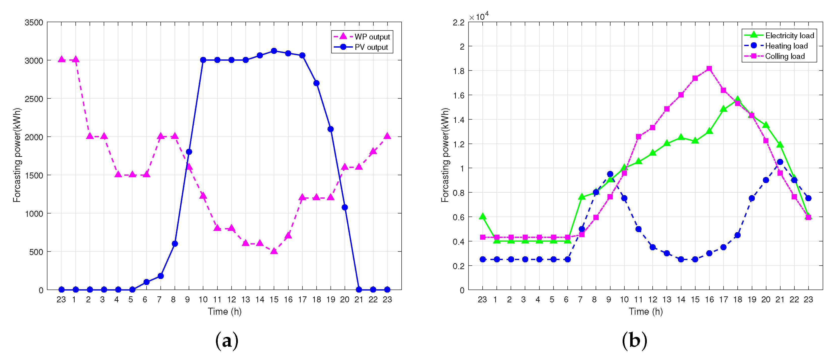
Thus far, we have completed the modeling framework of the variable performance parameters temperature–flowrate scheduling model for IES long-term economic planning. The scheduling model is to minimize the total operation cost and obtain the day-ahead scheduling plan at the hourly scale (11:00 p.m.–11:00 p.m. tomorrow) based on the forecast results of electricity, heating and cooling demands, and the PV/WT system’s output. The objective function is as follows:
F = t N T λ e ( t ) E G D ( t ) + t N T λ g a s F G T ( t ) + λ G T δ G T o n ( t ) + λ A C δ A C o n ( t ) + λ H P i n H P δ H P o n , i ( t ) + λ E C i n E C δ E C o n , i ( t )
where λ e ( t ) denotes the electricity price at time t, E G D ( t ) denotes the tie-line power at time t, λ g a s denotes the price of gas, λ G T / λ A C / λ H P / λ E C denote the startup penalty of different types of units, and N T represents the total hours of a scheduling period. Considering the startup penalty in the objective function can help to avoid frequent devices’ starting/stopping.
Constraints for the variable performance parameters’ temperature–flowrate scheduling model are as follows: (2)–(4), (6), (8)–(10), (12), (13),(16), (18), (20), (21), (23), (27), (28), (30)–(33), (36), (37), (39)–(44). All decision variables are shown in Table 2, and the values of parameters in the constraints or objective function are listed in Table 3 for the presented IES.
The proposed model can be solved by ILOG’s CPLEX 12.6 solver. The computation is performed on a tower-type server with an Intel Xeon CPU E5-2603 v3 @1.60 GHz processor and 8 GB RAM.

4. Case Study

4.1. Forecast Output of Renewables and Loads

In this section, the IES for an airport in Xi’an, a northwestern city in China, is used as a case study to verify the optimal model and compare the optimization results. Capacity of devices and energy supply methods of IES are shown in Table 1 and Figure 1. The proposed method is applied to obtain the day-ahead dispatch schedule on a representative day (15 August 2020). The scheduling period is from 11:00 a.m. today to 11:00 p.m. tomorrow. The Time-Of-Use (TOU) tariff presents the peak-valley-flat characteristic, the valley period is the first eight scheduling hours (11:00 p.m.–7:00 a.m.), the peak period is 9:00 a.m.–12:00 p.m. and 7:00 p.m.–11:00 p.m., and the other time is the flat period. The scheduling interval is 1 h.
The energy forecasts of the supply and demands are performed by adopting the prediction algorithm in [33]. The forecast outputs of wind power and photovoltaic power on this representative day are shown in Figure 6a:
With the given penetration of solar energy and photovoltaic power, the load forecasts of the demands on this representative day are depicted in Figure 6b.

4.2. Results and Discussion

In order to prove the superiorities of the proposed model, a comparative study is conducted by applying two models. Case 1 is the scheduling model in [32] and Case 2 is our proposed method, the essential difference is:
Case 1: temperature and flowrate are taken as decision variables, but all the performance parameters are all treated as constants. The C O P E C i , C O P H P i , η G T , η W H B are assumed to be 6.0, 5.0, 28%, and 80%, respectively.
Case 2: temperature and flowrate are taken as decision variables, while considering the variable performance parameters. The COPs of HP/EC are influenced by the outlet temperature and partial load factor, and the η G T , η W H B are influenced by the partial load rate.
Considering that the models in these two cases are all thorough temperature–flowrate based scheduling models, the scheduling result will be discussed from two different perspectives. The first part is the comparison results and discussion from the perspective of energy analysis, and the second part is from the perspective of the temperature and flowrate analysis.

4.2.1. Energy Analysis

Based on the scheduling model in the aforementioned two cases, this section presents and analyzes the comparison operation results from the perspective of energy analysis. Optimization results of the electrical power output, cooling power output, and heating output of each device of Case 1 are shown in Figure 7, and optimization results of Case 2 are shown in Figure 8. Scheduling models in two cases all obtain reasonable dispatch results, and the commonness of the comparison operation results will be discussed firstly.
Figure 7a and Figure 8a show the electrical power allocation among multiple devices of Case 1 and Case 2, respectively. In the valley period of the electricity price, the power of renewable energy power generation is relatively low, the system purchases electricity from the power grid to fulfill the demand of electricity, and the excess electricity is charging into BA at the same time to store energy for the peak-period power supply. In the flat period, although the GT unit is in the on state, it is still necessary to purchase electricity from the power grid to meet the power demand, and the electrical demand is mainly supplied by the power grid, renewable energy power, and the GT. In the peak period, the electricity demand is mainly satisfied by the renewable energy power, GT, and the discharge power of BA, and the insufficient electricity demand will be balanced by the power grid.
Figure 7b and Figure 8b demonstrate the optimal heating allocation among multiple devices of Case 1 and Case 2, respectively. From 11:00 p.m. to 6:00 a.m. tomorrow, the heating load is small, only one HP is in operation to fulfill the demand of basic heating load. From 7:00 a.m. to 9:00 a.m., the heating load is increasing and reached its first peak, the GT is turned on, so the WHB exerts the remaining thermal effects to meet part of the heating demand concomitantly, and both HPs are put in operation to meet the insufficient heating demand. After that, the heating load falls back and only one HP unit is in the ON state when the executing power is relatively small. From 6:00 p.m. to 10:00 p.m., the heating load reaches its second peak and the heating demand is supplied by the two HPs and the WHB simultaneously.
Figure 7c and Figure 8c describe the cooling power allocation among multiple devices of Case 1 and Case 2, respectively. In the valley period, the cooling demand is mainly supplied by EC, and TA is in cooling-storage mode at the same time to store the excessive cold water. In the first flat period (from 7:00 a.m. to 9:00 a.m.), EC units are the main cooling suppliers. In the first peak period (from 9:00 a.m. to 12:00 p.m.), the TA begins to execute the cooling order by discharging cold water, the AC serves as the complementary suppliers. In the second flat period (from 12:00 p.m. to 7:00 p.m.), the cooling demand is mainly satisfied by the AC and EC, and the insufficient demand will be supplied by the discharge cold water of TA. From 7:00 p.m. to 11:00 p.m., the TA discharges completely and the EC covers the cooling deficit.
Figure 7d and Figure 8d show the curves of the energy stored in the TA and the BA of Case 1 and Case 2, respectively. In the valley period, the TA operates in water storage mode. In the non-valley period, the TA executes the cooling mode. Plainly, the TA discharges more cooling energy in the peak period to reduce the total energy costs. As for BA, limited by the energy storage, BA can not achieve the energy supply in all non-valley periods of power consumption. In order to realize maximum profitability, the discharging periods of BA coincide with the two periods of high electricity price, i.e., 9:00 a.m. to 12:00 p.m. and 7:00 p.m. to 11:00 p.m.
Consequently, from the above analysis, both two optimization dispatching models have significantly improved the utilization of energy storage device and minimize the expectation of operation costs. However, several critical details differ in these two cases. Firstly, the load rates of all EC units in two modes are shown in Figure 9. In Case 1, because the COPs of ECs are simplified as constants and do not vary with the partial load rate, the change range of load rates are large. Comparatively, in Case 2, the load rates of all ECs are all in the range of 70% to 100%, which is the high COP domain of the EC (see Figure 4), Secondly, the number of EC units in the on state in two cases is shown in Figure 10. It can be found that, in Case 1, all the EC units are always in operation regardless of whether the cooling load is high or low. This is because, in Case 1, the COP does not vary with the partial load rate, so the operation result tends to put all the EC units in operation to avoid the startup penalty. Comparatively, the operation result of Case 2 will regulate the on-state EC numbers in order to ensure the high COP operation for each unit in operation. Therefore, this indicates that the simplistic assumption of the invariable COP in Case 1 could lead to a radical operational strategy. Obviously, our method shown in Case 2 is more superior and appropriate in engineering practice.

4.2.2. Flowrate and Temperature Analysis

From the perspective of flowrate and temperature analysis, the comparison between two cases provides that operation results will change significantly when considering the variable COPs of HP/EC and efficiency of GT/WHB. Taking EC units as examples, the temperature and flowrate scheduling results of EC for two cases are depicted in Figure 11a–c. It can be seen that the water temperature setpoint calculated in Case 1 is generally lower than that in Case 2 for every EC units, and the flowrate setpoint calculated in Case 1 is also lower than that in Case 2. This is because the COP is treated as constant and not affected by the temperature for Case 1, so the operation result of Case 1 tends to be a big temperature difference with a small water flowrate to reduce the pumping power. This leads to the outlet temperature setpoint being lower because the inlet water temperature is fixed. Comparatively, in the proposed model in Case 2, as the increase of the temperature, there is an increase in the COP of the EC, and correspondingly there is also an increase in the pumping power because of a big water flowrate. Due to a comprise of the pumping power and the COP, the operation results of Case 2 get a trade-off between the temperature difference and flowrate at the same cooling energy output. In other words, although the pumping power consumption is more than that in Case 1, the operation result in Case 2 is still an optimal solution.
To further elucidate the differences, the actual COP at different times of two cases are plotted in Figure 12, which can be calculated by Equation (24). It can be seen that COPs in Case 2 remain at a high level, whereas COPs in Case 1 fluctuate dramatically and are well below the assumed value 6.5, and the implementation process in practice will not accord with scheduling results in Case 1, suggesting the necessity of accommodating the variation of the COP.
In the same way, the temperature and flowrate scheduling results of HPs for two cases are depicted in Figure 13. It can be shown that the operation results of Case 1 tend to have a big temperature difference with the small water flowrate, which means, at a fixed inlet temperature, the outlet hot water temperature is generally higher and the flowrate is less than that in Case 2. The operation results of Case 2 can obtain a trade-off between the high pumping power consumption and high COP.
It should be noted that the trends of the outlet temperature of the heat exchanger attached to WHB and HP are opposite because their mixed temperature has to be within the range of upper and lower limits [ T H m i n , T H m a x ] . As shown in Figure 14a, the outlet temperature of WHB in Case 2 stabilizes at 70.5 °C and is higher than that in Case 1. This is because the efficiency of the plate heat exchanger is not affected much by the outlet temperature (in this paper, the efficiency of the plate heat exchanger is assumed to be constant).Their mixed temperature in a hot network is shown in Figure 14b, which investigates the hot network temperature in Case 2 being stable with little fluctuation and slightly lower than that in Case 1. In Case 2, on the one hand, the pumping power of the plate heat exchanger is reduced because of the increase of its outlet temperature. On the other hand, the HP units achieve lower outlet temperature and thus improve the COP. Therefore, considering the variable COP makes the scheduling results more effective and the economic benefits more favorable
Similarly, as shown in Figure 15a, the outlet temperature of AC in Case 2 stabilizes at a lower temperature. This is because the COP of the AC are not affected much by the outlet temperature (in this paper, the COP of the AC are assumed constant), decreasing the outlet temperature of the AC properly can help to achieve higher outlet temperature and thus improve the COP of the EC units. In addition, because the outlet temperature of AC is nearly the same and the outlet temperature of EC is much higher for Case 2, the cold network temperature in Case 2 is higher than that in case 1 as shown in Figure 15b.
The above analysis shows that the simplistic assumption of the invariable performance parameters could make the operational strategy uneconomic and inconsistent with the actual situations, and the variability of some performance parameters, like the COP or efficiency, should not be underestimated in IES, and the variable performance parameters temperature–flowrate scheduling model can account for such influence suitably.

5. Conclusions

This work addresses the optimal scheduling of the IES. Conventional MILP scheduling models of IES suffer from one or both of the following limitations: (1) Models are usually established without considering the variability of performance parameters. However, performance parameters like the COP of chillers vary over a wide range for various factors in practical. Therefore, the actual implementation process will not accord with the scheduling result when performance parameters are taken as constants. (2) Most of the models are energy-transfer based scheduling models, which are established by taking the energy transfer as decision variables rather than the temperature and flowrate, so energy-transfer based scheduling models can not take the impact of water temperature on performance parameters into account, and the scheduling results can not be directly applied to the control device.
In order to make the actual implementation process accord with the strategy of the scheduling model and take the impact of water temperature on performance parameters into account, the present paper proposes a variable performance parameters temperature–flowrate scheduling model, in which performance parameters are treated as variables rather than constants. The efficiencies of the gas turbine and the waste heating boiler are estimated with the partial load factor, and COPs of the electrical chillers and heat pumps are estimated with the partial load factor and outlet water temperature. Subsequently, a linearization technique called a COP-expansion method is also developed by adopting a specific representation of COP and the expansion of the outlet water temperature. Thus, the impacts of water temperature and part load factor on COPs are taken into account simultaneously in the scheduling model.
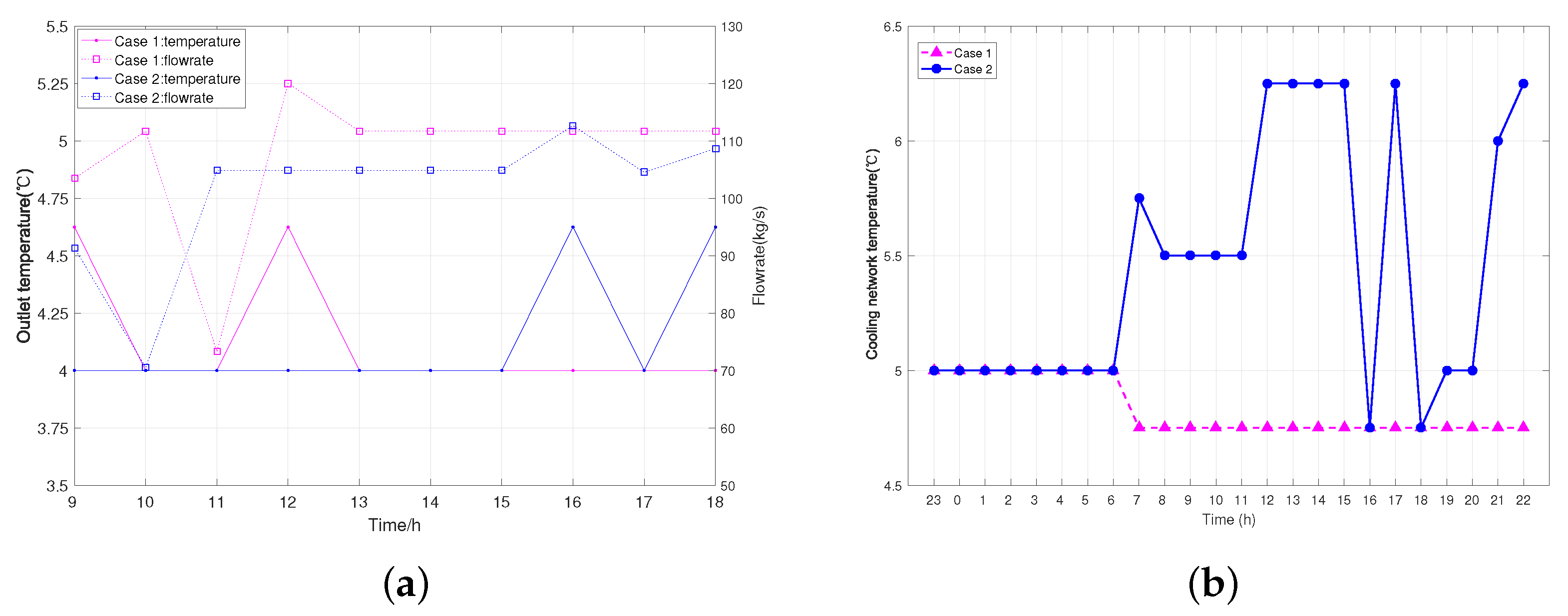
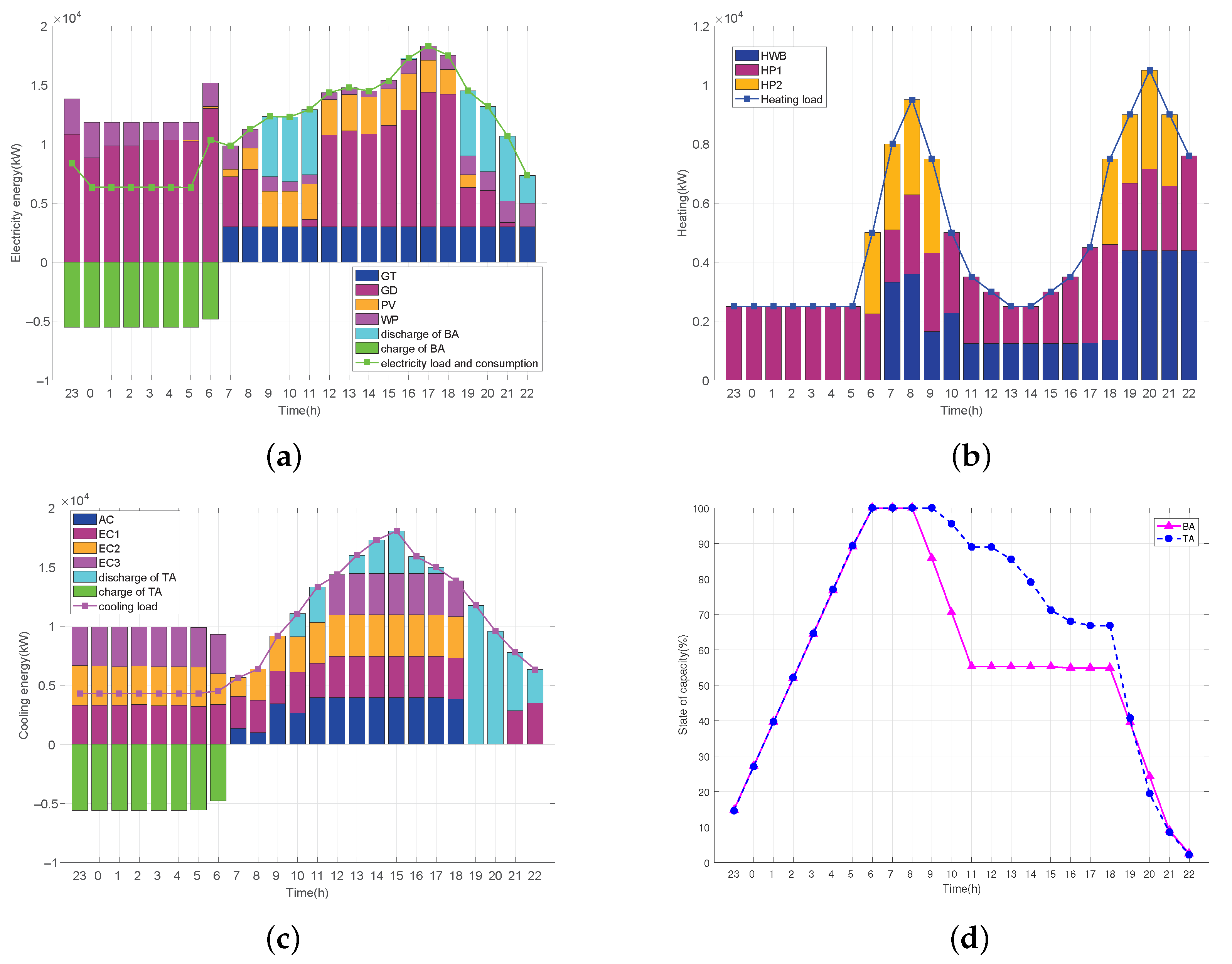
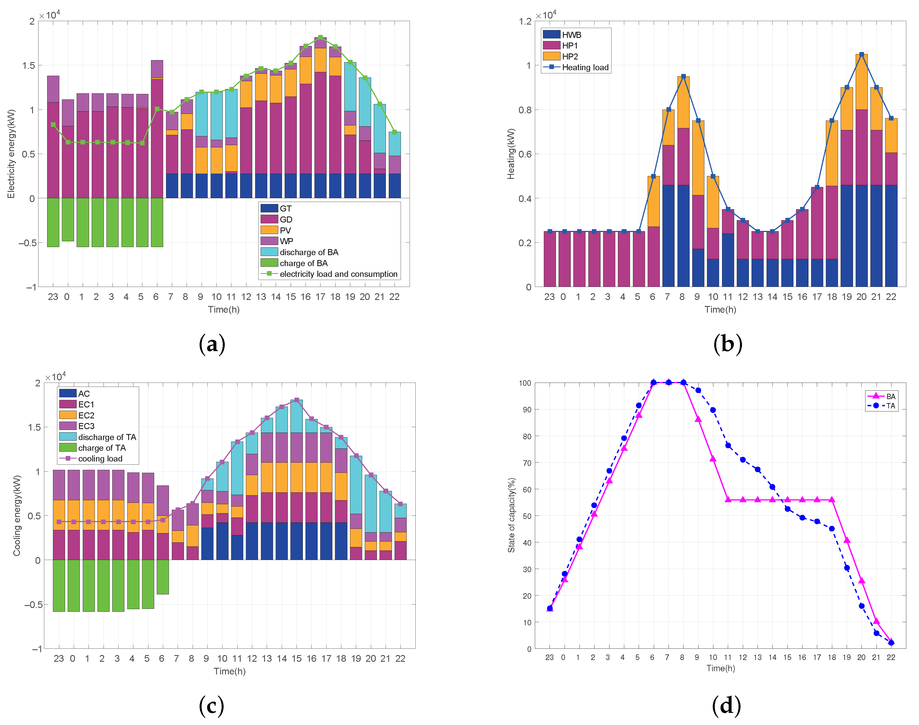
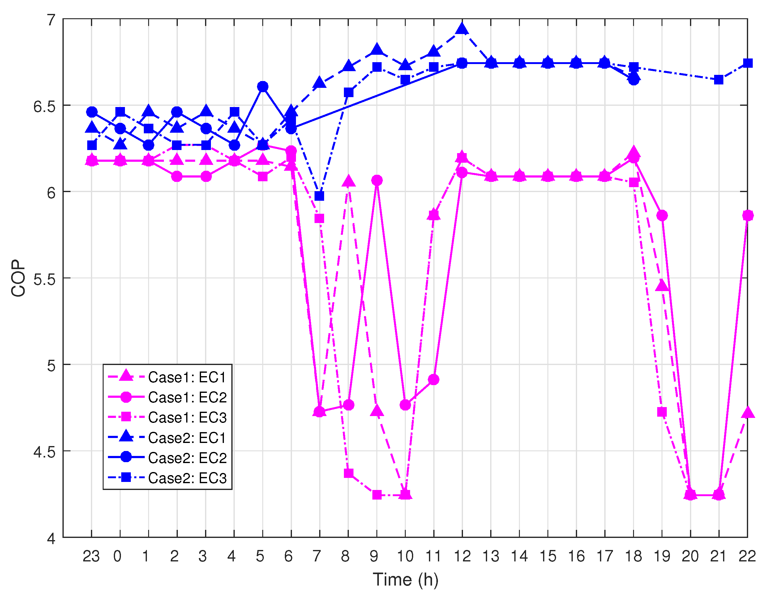
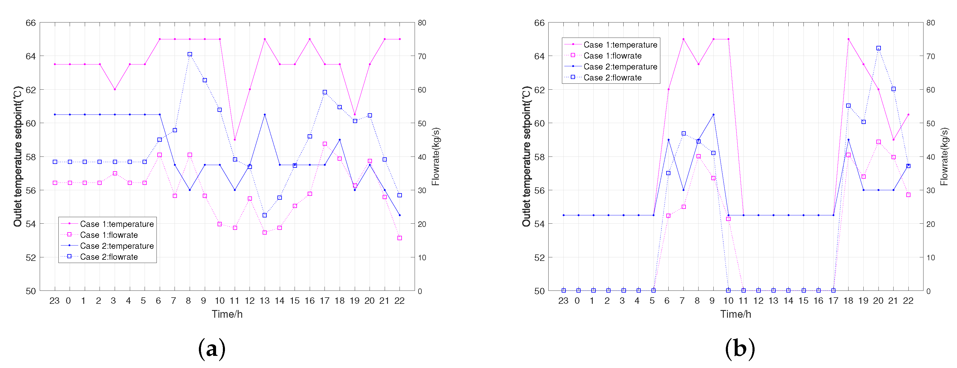
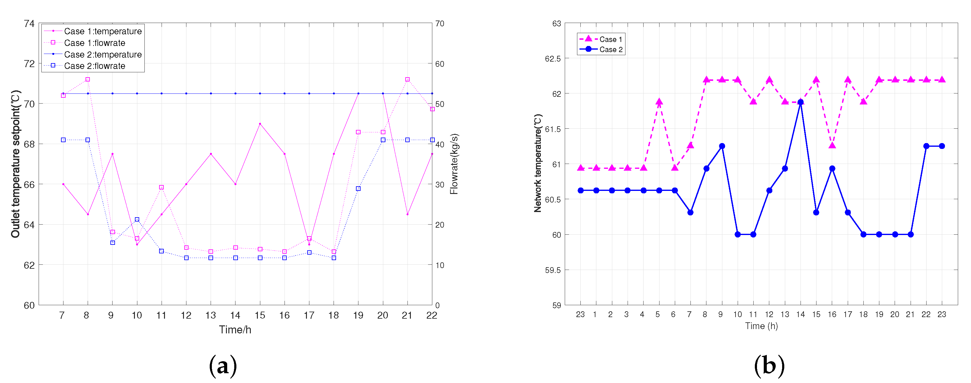
An IES in Xi’an in China is used to verify the optimal model and compare the optimization results. The proposed method is applied to obtain the day-ahead dispatch schedule on a representative day. In addition, a comparative study is conducted by applying two cases; in the first case, all the thermal performance parameters are all treated as constants, and, in the second case, the variable of performance parameters is considered. The comparison analysis has been conducted from two different perspectives: the energy analysis and the temperature and flowrate analysis. From the perspective of energy analysis, the simplistic assumption of the invariable performance parameters could lead to a radical operational strategy. From the perspective of flowrate and temperature analysis, the comparison shows that taking performance parameters as constants is over-simplified and can not accord with the true condition.
In conclusion, the proposed novel temperature–flowrate based scheduling model has two-fold merits: (1) The proposed scheduling model is established that directly takes temperature and flowrate as decision variables, which means that the scheduling results can be directly applied to control devices; and (2) performance parameters are treated as variables in the proposed scheduling model; for example, the COPs of the electrical chiller and heat pump are estimated with the partial load factor and water temperature collectively.
The variability of thermal performance parameters can also be represented as another form or we can take more influencing factors into account in the framework, which will be addressed in our future work.

Author Contributions

Conceptualization: H.-H.N. and Y.-G.L.; methodology: H.-H.N. and Y.Z.; software: H.-H.N. and S.-S.W.; validation: H.-H.N. and Y.Z.; formal analysis: S.-S.W.; investigation: H.-H.N.; resources: Y.-G.L.; data curation: H.-H.N.; writing—original draft preparation: H.-H.N. and Y.Z.; editing: Y.Z.; visualization: Y.Z.; supervision: Y.-G.L.; project administration: Y.-G.L.; funding acquisition: H.-H.N. and Y.-G.L. All authors have read and agreed to the published version of the manuscript.

Funding

This research was funded by the National Key Research and Development Program of China, Grant No. 2018YFB1502904 and National Natural Science Foundation of China, Grant No. 51936003.

Institutional Review Board Statement

Not applicable.

Informed Consent Statement

Not applicable.

Data Availability Statement

Data available on request.

Conflicts of Interest

The authors declare no conflict of interest.

Abbreviations

The following abbreviations are used in this manuscript:
ACAbsorption chiller
BABattery
CCHPCombined cooling, heating, and power
COPCoefficient of performance
ECElectrical chiller
FELFollowing electric load
FTLFollowing thermal load
GDPower grid
GTGas turbine
HPHeat pump
IESIntegrated energy system
MILPMixed integer linear programming
MNILPMixed integer nonlinear programming
PVPhotovoltaic array
TAWater tank
TOUTime-of-use
WHBWaste heat boiler
WPWind power

References

  1. Saari, A.A. Distributed energy generation and sustainable development. Renew. Sustain. Energy Rev. 2006, 10, 539–558. [Google Scholar]
  2. Wu, D.W.; Wang, R.Z. Combined cooling, heating and power: A review. Prog. Energy Combust. Sci. 2006, 32, 459–495. [Google Scholar] [CrossRef]
  3. Wei, S.; Li, Y.; Gao, X. Multi-stage Sensitivity Analysis of Distributed Energy Systems: A Variance-based Sobol Method. J. Mod. Power Syst. Clean Energy 2020, 8, 895–905. [Google Scholar] [CrossRef]
  4. Mago, P.J.; Chamra, L.M.; Ramsay, J. Micro-combined cooling, heating and power systems hybrid electric-thermal load following operation. Appl. Therm. Eng. 2010, 30, 800–806. [Google Scholar] [CrossRef]
  5. Fang, F.; Wang, Q.H.; Shi, Y. A novel optimal operational strategy for the cchp system based on two operating modes. IEEE Trans. Power Syst. Publ. Power Eng. Soc. 2012, 27, 1032–1041. [Google Scholar] [CrossRef]
  6. Wang, J.; Sui, J.; Jin, H. An improved operation strategy of combined cooling heating and power system following electrical load. Energy 2015, 85, 654–666. [Google Scholar] [CrossRef]
  7. Zhang, X.; Sato, A.; Kudo, Y.; Nakamura, T.; Majid, M. A case study of electric chiller performance bottleneck diagnosis by root cause analysis. In Proceedings of the 2016 1st International Conference on Information Technology, Information Systems and Electrical Engineering (ICITISEE), Yogyakarta, Indonesia, 23–24 August 2016. [Google Scholar]
  8. Matjanov, E. Gas turbine efficiency enhancement using absorption chiller: Case study for tashkent chp. Energy 2020, 192, 1–10. [Google Scholar] [CrossRef]
  9. Chen, G.; Cheng, X. Analysis of screw chiller’s refrigeration performance under large temperature difference cooling-water. Appl. Mech. Mater. 2014, 501, 2319–2322. [Google Scholar] [CrossRef]
  10. Yamamoto, T.; Hayama, H.; Hayashi, T. Formulation of coefficient of performance characteristics of water-cooled chillers and evaluation of composite cop for combined chillers. Energies 2020, 13, 1182. [Google Scholar] [CrossRef] [Green Version]
  11. Li, G.; Zhang, R.; Jiang, T.; Chen, H.; Bai, L.; Cui, H.; Li, X. Optimal dispatch strategy for integrated energy systems with cchp and wind power. Appl. Energy 2016, 192, 408–419. [Google Scholar] [CrossRef]
  12. Arcuri, P.; Florio, G.; Fragiacomo, P. A mixed integer programming model for optimal design of trigeneration in a hospital complex. Energy 2016, 32, 1430–1447. [Google Scholar] [CrossRef]
  13. Zl, A.; Yz, B.; Xw, A. Long-term economic planning of combined cooling heating and power systems considering energy storage and demand response. Appl. Energy 2020, 279. [Google Scholar]
  14. Aidong, Z.; Qingshan, X.; Kai, W.; Ling, J.; Xudong, W. A day-ahead optimal economic dispatch schedule for multi energy interconnected region. Energy Procedia 2016, 100, 396–400. [Google Scholar] [CrossRef] [Green Version]
  15. Kuang, J.; Zhang, C.; Fan, L.; Bo, S. Dynamic optimization of combined cooling, heating, and power systems with energy storage units. Energies 2018, 11, 2288. [Google Scholar] [CrossRef] [Green Version]
  16. Wang, C.; Lv, C.; Peng, L.; Song, G.; Li, S.; Xu, X.; Wu, J. Modeling and optimal operation of community integrated energy systems: A case study from china. Appl. Energy 2018, 230, 1242–1254. [Google Scholar] [CrossRef]
  17. Ma, T.; Wu, J.; Hao, L. Energy flow modeling and optimal operation analysis of the micro energy grid based on energy hub. Energy Convers. Manag. 2017, 133, 292–306. [Google Scholar] [CrossRef]
  18. Somma, M.; Yan, B.; Bianco, N.; Graditi, G.; Luh, P.B.; Mongibello, L.; Naso, V. Operation optimization of a distributed energy system considering energy costs and exergy efficiency. Energy Convers. Manag. 2015, 103, 739–751. [Google Scholar] [CrossRef]
  19. Chen, K.; Pan, M. Operation optimization of combined cooling, heating, and power superstructure system for satisfying demand fluctuation. Energy 2021, 237, 12–15. [Google Scholar] [CrossRef]
  20. Ma, W.; Fang, S.; Liu, G. Hybrid optimization method and seasonal operation strategy for distributed energy system integrating cchp, photovoltaic and ground source heat pump. Energy 2017, 141, 1439–1455. [Google Scholar] [CrossRef]
  21. Lu, Y.; Wang, S.; Sun, Y.; Yan, C. Optimal scheduling of buildings with energy generation and thermal energy storage under dynamic electricity pricing using mixed-integer nonlinear programming. Appl. Energy 2015, 147, 49–58. [Google Scholar] [CrossRef]
  22. Li, F.; Sun, B.; Zhang, C.; Zhang, L. Operation optimization for combined cooling, heating, and power system with condensation heat recovery. Appl. Energy 2018, 230, 305–316. [Google Scholar] [CrossRef]
  23. Li, F.; Sun, B.; Zhang, C.; Liu, C. A hybrid optimization-based scheduling strategy for combined cooling, heating, and power system with thermal energy storage. Energy 2019, 188, 115–948. [Google Scholar] [CrossRef]
  24. Rong, Z.A.; Xz, B.; Yan, D.C.; Hl, D.; Gz, D. Optimization and performance comparison of combined cooling, heating and power/ground source heat pump/photovoltaic/solar thermal system under different load ratio for two operation strategies. Energy Convers. Manag. 2020, 208, 112579. [Google Scholar]
  25. Wu, J.Y.; Wang, J.L.; Li, S. Multi-objective optimal operation strategy study of micro-cchp system. Energy 2012, 48, 472–483. [Google Scholar] [CrossRef]
  26. Moretti, L.; Manzolini, G.; Martelli, E. Milp and minlp models for the optimal scheduling of multi-energy systems accounting for delivery temperature of units, topology and non-isothermal mixing. Appl. Therm. Eng. 2012, 184, 116–125. [Google Scholar]
  27. Li, Z.; Yan, X. Optimal coordinated energy dispatch of a multi-energy microgrid in grid-connected and islanded modes—sciencedirect. Appl. Energy 2018, 210, 974–986. [Google Scholar] [CrossRef]
  28. Jiang, Y.; Xu, J.; Sun, Y.; Wei, C.; Wang, J.; Ke, D.; Li, X.; Yang, J.; Peng, X.; Tang, B. Day-ahead stochastic economic dispatch of wind integrated power system considering demand response of residential hybrid energy system. Appl. Energy 2017, 190, 1126–1137. [Google Scholar] [CrossRef]
  29. Luo, Z.; Wu, Z.; Li, Z.; Cai, H.Y.; Li, B.J.; Gu, W. A two-stage optimization and control for cchp microgrid energy management. Appl. Therm. Eng. 2017, 135. [Google Scholar] [CrossRef]
  30. Carrion, M.; Arroyo, J.M. A computationally efficient mixed-integer linear formulation for the thermal unit commitment problem. IEEE Trans. Power Syst. 2006, 21, 1371–1378. [Google Scholar] [CrossRef]
  31. Gu, W.; Wang, J.; Lu, S.; Luo, Z.; Wu, C. Optimal operation for integrated energy system considering thermal inertia of district heating network and buildings. Appl. Energy 2017, 199, 234–246. [Google Scholar] [CrossRef]
  32. Wei, S.; Li, Y.; Sun, L. Stochastic model predictive control operation strategy of integrated energy system based on temperature–flowrate scheduling model considering detailed thermal characteristics. Int. J. Energy Res. 2017, 45, 4081–4097. [Google Scholar] [CrossRef]
  33. Niu, H.; Yang, Y.; Zeng, L.; Li, Y. ELM-QR-Based nonparametric probabilistic prediction method for wind power. Energies 2021, 14, 701. [Google Scholar] [CrossRef]
Figure 1. Schematic configuration of the IES.
Energies 14 05400 g001
Figure 2. The efficiency curve of GT fitted by actual operating data.
Energies 14 05400 g002
Figure 3. The three-segment piecewise linear function curve of GT.
Energies 14 05400 g003
Figure 4. Diagram of the COP of the EC varied with the partial load rate under different outlet temperature setpoint T E C , o u t fitted by actual operating data.
Energies 14 05400 g004
Figure 5. Diagram of cooling output and electric energy input under different T E C , o u t .
Energies 14 05400 g005
Figure 6. The load forecast of demands and new energy power generation for the IES in Xi’an in China on 15 August 2020. The capacity of devices and energy supply methods of IES are shown in Table 1 and Figure 1. (a) the forecast output of wind power and photovoltaic power; (b) the load forecast of the demands.
Energies 14 05400 g006
Figure 7. The optimal generation scheduling results in Case 1 from the perspective of energy analysis. (a) the electrical power allocation among multiple devices; (b) the heating energy allocation among multiple devices; (c) the cooling energy allocation among multiple devices; (d) the curves of the energy stored in the TA and BA.
Energies 14 05400 g007
Figure 8. The optimal generation scheduling results in Case 2 from the perspective of energy analysis. (a) the electrical power allocation among multiple devices; (b) the heating energy allocation among multiple devices; (c) the cooling energy allocation among multiple devices; and (d) the curves of the energy stored in the TA and BA.
Energies 14 05400 g008
Figure 9. The operation load rate of all ECs in different mode. (a) Case 1; (b) Case 2.
Energies 14 05400 g009
Figure 10. The on-state number of all ECs in different cases.
Energies 14 05400 g010
Figure 11. The operation result of all ECs from the perspective of flowrate and temperature analysis. (a) the temperature and flowrate results of EC1; (b) the temperature and flowrate results of EC2; (c) the temperature and flowrate results of EC3.
Energies 14 05400 g011
Figure 12. The curves of COPs of all ECs in different cases.
Energies 14 05400 g012
Figure 13. The operation result of HP from the perspective of flowrate and temperature analysis. (a) the temperature and flowrate results of HP1; (b) the temperature and flowrate results of HP2.
Energies 14 05400 g013
Figure 14. The operation result of WHB from the perspective of flowrate and temperature analysis. (a) the temperature and flowrate results of WHB; (b) the mixed temperature in hot networks.
Energies 14 05400 g014
Figure 15. The operation result of AC from the perspective of flowrate and temperature analysis. (a) the temperature and flowrate results of AC; (b) the mixed temperature in the cold network.
Energies 14 05400 g015
Table 1. Values of system parameters for IES.
ParameterValueParameterValue
[ E G T m i n , E G T m a x ] (kW)[1000, 3000] [ E G D m i n , E G D m a x ] (kW)[0, 1,000,000]
[ E B A , c h m i n , E B A , c h m a x ] (kW)[0, 5000] [ E B A , d i s m i n , E B A , d i s m a x ] (kW)[0, 5000]
[ S B A m i n , S B A m a x ] (kWh)[1000, 30,000] [ H W H B m i n , H W H B m a x ] (kW)[2600, 5000]
[ H H P m i n , H H P m a x ] (kW)[1100, 3400] [ Q A C m i n , Q A C m a x ] (kW)[1000, 5000]
[ Q T A , c h m i n , Q T A , c h m a x ] (kW)[2000, 15,000] [ Q T A , d i s m i n , Q T A , d i s m a x ] (kW)[2000, 15,000]
[ S T A m i n , S T A m a x ] (kWh)[1000, 70,000] [ Q E C m i n , Q E C m a x ] (kW)[760, 3500]
Table 2. Decision variables in the optimization for IES.
TypeVariable
binary variable δ G T , δ G T o n , δ B A , c h , δ B A , d i s , δ W H B , δ H P i , δ H P o n , i , δ A C , δ A C o n
δ T A , c h , δ T A , d i s , z W H B , k , z H P , k i , z H , k , z Q , k
continuous variable E G T , F G T , E B A , c h , E B A , d i s , S B A , E G D , H W H B I N , H W H B , h o t , H W H B , s t e a m
H H P i , H A C I N , Q A C , Q E C i , Q T A , c h , Q T A , d i s , S T A , v W H B , k , q W H B , E p u m p , W H B
q E C i , v E C , k i , z E C , k i , E p u m p , E C i , Q E C , b a s e i , q H P i , v H P , k i , w E C , k i , w H P , k i
E p u m p , H P i , H H P , b a s e i , q H , v H , k , q T A , c h , q T A , d i s , q Q , v Q , k , E p u m p
Table 3. Values of parameters in the IES in China.
ParameterValueParameterValue
μ G T 0.30 μ H P 0.30
μ E C 0.30 η r e c 0.80
η B A , d i s 0.85 η B A , c h 0.85
η T A , d i s 0.95 η T A , c h 0.95
λ g a s (CNY/kWh)2.30 λ E , p e a k (CNY/kWh)1.13
λ E , v a l l e y (CNY/kWh)0.38 λ E , f l a t (CNY/kWh)0.73
λ G T (CNY)1000 λ A C (CNY)500
λ H P (CNY)500 λ E C (CNY)500
S B A s t a r t (kWh)1000 S T A s t a r t (kWh)1000
c p (kJ/kg·K)4.20 C O P A C 1.20
( x G T 1 , x G T 2 ) (650, 850) ( k G T 1 , k G T 2 , k G T 3 ) (4.1655, 4.4991, 3.6722)
( x G T 0 , y G T 0 ) (500, 935)K3
[ T W H B , o u t m i n , T W H B , o u t m a x ] (°C)[60, 72] T W H B , i n ( t ) (°C) 45
q W H B m a x (kg/s)100 E p u m p , W H B m a x (kW)200
( x W H B 1 , x W H B 2 ) (4000, 5000) ( k W H B 1 , k W H B 2 , k W H B 3 ) (0.9603, 0.9619, 0.9089)
( x W H B 0 , y W H B 0 ) (3350, 2647) Δ T W H B (°C)1.5
[ T E C , o u t m i n , T E C , o u t m a x ] (°C)[4.5, 8.5] T E C , i n i ( t ) (°C)13
q E C m a x (kg/s)180 E p u m p , E C m a x (kW)250
( x E C 1 , x E C 2 ) (260, 410) ( k E C 1 , k E C 2 , k E C 3 ) (7.8681, 8.6745, 0.3334)
( x E C 0 , y E C 0 ) (160, 670.30) Δ T E C (°C)0.5
α E C 0.030 α H P 0.030
[ T H P , o u t m i n , T H P , o u t m a x ] (°C) [54.5, 66.5] T H P , i n i ( t ) (°C) 45
q H P m a x (kg/s)100 E p u m p , H P m a x (kW)200
( x H P 1 , x H P 2 ) (350, 500) ( k E C 1 , k E C 2 , k E C 3 ) (5.8755, 6.0440, 5.2240)
( x E C 0 , y E C 0 ) (225, 984.18) Δ T E C (°C)1.5
Δ T H (°C)0.625 Δ T Q (°C)0.375
[ T H m i n , T H m a x ] (°C)[60,65] q H m a x (kg/s)1000
[ T Q m i n , T Q m a x ] (°C)[5,8] q Q m a x (kg/s)1000
T T A (°C)5 T r e t , Q (°C)13
Publisher’s Note: MDPI stays neutral with regard to jurisdictional claims in published maps and institutional affiliations.

