Article

Energy Benefits of Heat Pipe Technology for Achieving 100% Renewable Heating and Cooling for Fifth-Generation, Low-Temperature District Heating Systems

1
Mechanical Engineering Department, Ostim Technical University, Ankara 06374, Turkey
2
Polar Project Technology, Informatics, Architecture, Engineering, Ankara 06640, Turkey
3
Enover Energy, Ankara 06510, Turkey
*
Author to whom correspondence should be addressed.
Energies 2021, 14(17), 5398; https://doi.org/10.3390/en14175398
Submission received: 14 May 2021 / Revised: 28 July 2021 / Accepted: 29 July 2021 / Published: 30 August 2021
(This article belongs to the Special Issue Thermal Comfort and Energy Use in Buildings)

Abstract

:
This paper addresses the challenges the policymakers face concerning the EU decarbonization and total electrification roadmaps towards the Paris Agreement set forth to solve the global warming problem within the framework of a 100% renewable heating and cooling target. A new holistic model was developed based on the Rational Exergy Management Model (REMM). This model optimally solves the energy and exergy conflicts between the benefits of using widely available, low-temperature, low-exergy waste and renewable energy sources, like solar energy, and the inability of existing heating equipment, which requires higher exergy to cope with such low temperatures. In recognition of the challenges of retrofitting existing buildings in the EU stock, most of which are more than fifty years old, this study has developed a multi-pronged solution set. The first prong is the development of heating and cooling equipment with heat pipes that may be customized for supply temperatures as low as 35 °C in heating and as high as 17 °C in cooling, by which equipment oversizing is kept minimal, compared to standard equipment like conventional radiators or fan coils. It is shown that circulating pump capacity requirements are also minimized, leading to an overall reduction of CO2 emissions responsibility in terms of both direct, avoidable, and embodied terms. In this respect, a new heat pipe radiator prototype is presented, performance analyses are given, and the results are compared with a standard radiator. Comparative results show that such a new heat pipe radiator may be less than half of the weight of the conventional radiator, which needs to be oversized three times more to operate at 35 °C below the rated capacity. The application of heat pipes in renewable energy systems with the highest energy efficiency and exergy rationality establishes the second prong of the paper. A next-generation solar photo-voltaic-thermal (PVT) panel design is aimed to maximize the solar exergy utilization and minimize the exergy destruction taking place between the heating equipment. This solar panel design has an optimum power to heat ratio at low temperatures, perfectly fitting the heat pipe radiator demand. This design eliminates the onboard circulation pump, includes a phase-changing material (PCM) layer and thermoelectric generator (TEG) units for additional power generation, all sandwiched in a single panel. As a third prong, the paper introduces an optimum district sizing algorithm for minimum CO2 emissions responsibility for low-temperature heating systems by minimizing the exergy destructions. A solar prosumer house example is given addressing the three prongs with a heat pipe radiator system, next-generation solar PVT panels on the roof, and heat piped on-site thermal energy storage (TES). Results showed that total CO2 emissions responsibility is reduced by 96.8%. The results are discussed, aiming at recommendations, especially directed to policymakers, to satisfy the Paris Agreement.

Graphical Abstract

1. Introduction and Literature Survey

1.1. Overview

Today any civilized action has a carbon footprint. To reduce the global warming rate, the legally binding Paris Agreement was signed by the World Leaders in December 2015, with the primary objective to keep the global temperature rise below 2 °C compared to pre-industrial levels until 2100. A further ambition is 1.5 °C [1]. However, Figure 1 indicates that these goals will not be achieved. According to the OECD Outlook Baseline Projects Report, without more ambitious policies yet to be developed, the greenhouse gas emissions (GHG) would reach almost 685 parts per million (ppm) CO2-equivalents by 2050. This concentration is well over the limit of 450 ppm (parts per million) to have at least a 50% chance of meeting the Paris Agreement goals [2].
CO2 never increased more than 30 ppm during the last thousand years, but it did so during the past twenty years and continuing [4]. Despite serious measures taken to reduce the CO2 emissions and other particulates, Figure 1 reveals that there must be a fundamental flaw in the current theory and applications due to a lack of understanding about the missing mechanism of the unexplained CO2 emissions, which is either unknown or ignored. In the year 2020, the ‘calculated’ global CO2 emissions exceeded 36 billion tons. This calculation was carried out based on different fractions of coal, oil, gas, and renewable energy sources worldwide, all of which have different unit content of CO2. This result is an outcome of such a simplistic calculation concerning only the supply side. However, no one asks where these fuels and energy sources are used and how exergy-rational the utilization rate of their useful work potential is. Exergy is the useful work potential (quality) of a given amount or flow of energy quantity. Energy may be stored and recovered. Exergy may not be stored or recovered but destroyed, according to the 2nd Law of thermodynamics. Therefore, when the term energy is used, it is accompanied by two vectors, namely the quantity and quality. According to the ideal Carnot Cycle, exergy is always less than the quantity of energy (Exergy = (1 − Tref/Tsup) times the energy quantity, and Tref > 0 K). For example, if natural gas, which has a useful work potential of 87% of its energy content and burns almost at 2000 °C, is simply used in a condensing boiler for comfort heating at 20 °C, then the rationality of spending such a valuable fuel only for heating on the demand side is only about 10%, although condensing boilers are generally claimed to be more than 95% efficient. Natural gas, for example, could be used in power generation, industry, and finally, the waste heat could be serviced to the buildings. Otherwise, almost 80% of the useful work potential is destroyed irreversibly in a condensing boiler in buildings. This destruction leads to additional CO2 emission responsibility. This responsibility is the missing part of the strategies for decarbonization and is a simple matter of recognition of the 2nd Law for energy quality, exergy.
Someone, somewhere, sometime, and by some means, will need to offset the exergy destructions with additional fuel spending and effort. In other words, we ‘calculate’ the direct emissions but ignore the additional emissions responsibilities, which take place due to mismatches of useful work potential (Exergy Destruction) between the supply and demand. Recognition of the relationships among energy, exergy, exergy destructions, and nearly-avoidable CO2 emissions is critical in emissions control for taking a sustainable position against climate emergencies [5]. Some concerned scientists and engineers have first announced the importance of exergy in the EU by releasing an opinion paper in 2016, with a ‘Think Exergy, not Energy’ [6]. They explained the concept of exergy and its application to energy efficiency, reaching out to policymakers to call for the formation of an International Exergy Panel to specifically address exergy destructions and their implications on the environment. Although this panel did not materialize, it generated enough interest for partial recognition of the importance of the 2nd Law of Thermodynamics. The EU is preparing new roadmaps to mobilize low-exergy (temperature) resources like waste heat, low-temperature solar heat, and low-enthalpy geothermal energy resources. These are widely available but untapped so far. Among various opportunities, buildings, representing almost 40% of the global energy consumption and a similar rate of CO2 emissions, present the largest asset of decarbonization efforts by utilizing such low-exergy sources on the horizon.

1.2. Buildings and the Environment

In many EU countries, half of the residential stock comprises buildings, which were built before 1970, when the first thermal efficiency regulations were not in place yet [7]. This situation is almost the same for all other countries with exceptions like Spain and Ireland. Since such existing buildings are still energy-inefficient despite thermal over-insulation retrofits, their thermal loads are still high. They run on old heating equipment like steel or even cast-iron radiators or natural-convection coils, which were designed for high supply temperatures. Therefore, there is a significant conflict between the many old buildings that demand high supply temperatures and the new EU roadmap of utilizing low-temperature thermal sources. Old hydronic heating equipment was designed for at least 70 °C of supply design temperature (Teq). Nowadays, the EU is considering moving towards ultra-low temperature district energy systems with temperatures as low as 35 °C (Tsup) [8,9]. In the Framework of International Energy Agency (IEA) Annex 37, a comprehensive compilation of research was carried out by IEA on low-temperature heating and its potential implications and the so-called side effects [10]. They argued that adding passive building systems for better retaining of solar gains and other internal sources, a continuous but lower thermostat settings shave off the peak loads and somehow enhance the utilization of low-temperature heat supplies. They considered floor heating, wall heating, oversized radiators and convectors, and air heating. Their studies were not too conclusive about energy performance, which were limited to the 1st Law of Thermodynamics only, and they did not investigate the effect of district piping and pumping on energy benefits or disadvantages. The potential impacts of low-temperature heating from the perspective of buildings about indoor air quality (IAQ), comfort, and energy have been further investigated by Eijdems, Boerstra, and Veld, without considering the conflict between energy supply temperature and the equipment demand temperature [9]. For public understanding and acceptance, they termed the low-exergy (Low-Temperature) energy as ‘low valued’ energy. They overviewed the impact of low-temperature supply to heating equipment for several types of equipment, including radiant floor and wall panels, low-temperature air heating. They qualitatively claimed that IAQ and sensation of comfort improve mainly by using radiant panels, which already permit low temperatures for operation. However, they did not study how low-temperature heating may be made possible by designing new equipment and or existing oversizing equipment, except noting that heat pump COP values may increase due to reduced temperature deficit between the supply and demand [9]. Figure 2 models this conflict of at least 35 °C of temperature deficit. When a low-temperature source is provided at Tsup, Figure 2 also shows that over insulation of the old buildings may reduce the gap.
Figure 2 is a 2-D graphical representation of the exergetic relationship among temperatures, namely ΔT, Tref, Ta, and T`sup (Exergy Triangle). The side between points TaTref represents the unit demand exergy. The side (T`supTref) represents the unit supply exergy. The side Ta(T`sup − 1/2 ΔT) represents the exergy of a unit thermal load (Q = 1 kW), EXH. The triangular area Δs represents the optimization objective, which needs to be maximized within the given temperature constraints and given design temperatures. For a detailed explanation of Figure 2, please refer to Appendix A.
According to Figure 2, at an indoor comfort temperature of Ta and the rated supply temperature requirement of the conventional heating equipment, Teq, there is a temperature deficit between the low-temperature district supply, Tsup, and Teq. The thermal load, Q, may be reduced by additional thermal insulation (Over insulation). This measure also reduces Teq to T`eq, reducing the temperature gap between the thermal supply and equipment requirements. However, over insulation has both economic and thermophysical limits, and therefore over insulation is a weak tool to resolve the problem. It is possible to determine an optimum relation between the over-insulation and equipment oversizing by referring to the Rational Exergy Management Efficiency (REMM), ψR [11]. The term ψR is the key for sustainably meeting the Paris Agreement goals because it is an indicator of nearly-avoidable CO2 emissions, namely ΔCO2, emanating from exergy destructions (εsup − εdem). Any mismatch is reflected upon ψR. The term ψR has been defined by the ideal Carnot Cycle applied to the unit exergy demand, εdem, and the unit exergy supply from source to equipment, εsup.
ψ R = ε d e m ε s u p = ( 1 T r e f T a ) ( 1 T r e f T s u p ) + ( 1 T s u p T e q ` )         ( Maximize .   Exergy - Based )
For maximum ψR, the denominator may be minimized if Ta is fixed. By differentiating the denominator concerning Tsup and then equating it to zero:
T e q ` = T s u p 2 T r e f         ( For   Maximum   ψ R )
Δ T e q ` 2 T s u p Δ T s u p Δ T s u p Δ T e q ` 2 T s u p
Tref is the reference environment temperature. A fixed value of 283 K in heating and 273 K in cooling were selected as common bases for all analyses. Then, the exergy-based (Equation (2)) sensitivity for maximum rationality at a given supply temperature is proportional to the uncertainties in the supply temperature, and it is twice as much. Therefore, for a narrow margin of sensitivity required about the maximum ψR at low supply temperatures as desired by the EU roadmaps, uncertainties in the supply temperature must be minimal. This is a critical issue for control systems of 5DE districts with renewables in terms of exergy because Tsup is low, and ΔT`eq must also be kept minimum, making the condition hard to satisfy. Figure 3 shows the trend of variables according to different Tsup values. Maximum possible exergy rationality, ψR, which is 0.40 is obtained at Tsup = 30 °C. At this supply temperature, the insulation must be too heavy that the Q` will be about 50% of the design heating load, which is not practical. If Tsup is 35 °C (308 K) and the reference temperature is 283 K, then T`eq is 335 K (62 °C) for maximum ψR at these temperatures. If Ta = 24 °C (297 K), ψR will be:
ψ R = ε d e m ε s u p = ( 1 283   K 297   K ) ( 1 283   K 308   K ) + ( 1 308   K 335   K ) = 0.0471 0.1617 = 0.291
The over-insulation rate is implicitly given by Equation (3). (n) is the equipment heating capacity exponent [12]. Tsup0 is the original supply design temperature of the heating equipment, like 70 °C.
( % Q ` Q ) = ( ( T e q ` T a ) ( T s u p 0 T a ) ) n × 100
Equation (3) provides the energy-based implicit sensitivity of the thermal conditioning load with a change in equipment n, which is a function of changing indoor conditions and the supply temperature as discussed above in Equation (2). If the original heat load coefficient of the building, U0, is known, then the need for over insulation may be estimated from Equation (4). To is the outdoor design temperature. Decreasing U` is also an optimality condition for heat pump COP (See Section 2.4.3).
U ` U 0 = ( T e q ` T o ) ( T s u p 0 T o )
For example, if Tsup is 35 °C, buildings need to be insulated such that their heating loads are reduced by about 78%. Then the value is locally maximized to 0.29 (29% on the graph). At Tsup = 39 °C, no additional insulation is necessary. This simple exergy-based model shows how the exergy analysis may be effective. For example, now a designer may choose whether to insulate the building more or choose a higher supply temperature mix or blend of waste heat or go deeper in geothermal well if low-enthalpy geothermal energy is to be used.
As depicted in Figure 4, district or central comfort heating in the industrial era dates back to the 1880s, mainly starting with generating and distributing steam for heating in a district loop or individual buildings around 200 °C (473 K). This step is the first-generation district energy system (1DE or 1G). The exergy rationality of steam in heating is very low. compared to modern systems, as the following equation gives, ψR to be 0.117, which is significantly less than 0.70, which is the limit for green districts [11]:
ψ R = ε d e m ε s u p = ( 1 283 273.15 + 24 ) 0.406 = 0.117       ( Steam   to   comfort )
where the unit exergy of steam, εs is approximated by the following equation:
ε s 0.00198 ( T s 283   K )       ( Steam )
An equivalent (Virtual) Carnot Cycle-based energy source temperature, Tf may be defined for steam by simply equating εs from Equation (6) to (1 − Tref/Tf):
Building insulation plays an important role in green certification programs [13]. However, these programs ignore the connection between thermal insulation and other components of a green building like a heat pump. If a heat pump is used, over insulation as favorably presented in Figure 2 may seem economically unfeasible and not worth any further green points. However, when the performance improvement of the heat pump and the positive impact on emissions is considered, the optimum insulation value shifts favourably.
The vertical black line corresponds to the point where Q`, which is seen in shown in Figure 3, is equal to the original thermal load, Q (No over insulation). This line crosses the original equipment supply temperature requirement (70 °C, no oversizing), shows a minimal ψR of about 0.23, and indicates that the supply temperature may be less than about 39 °C to allow for better exergy rationality and give some room for over insulation.
At a superheated steam temperature, TS of 488 K at a pressure of 20 bar εsup is 0.406 kW/kW, and Tf is 476.4 K, which is very close to TS in this case. On the other hand, if moderate-quality coal with unit exergy of 0.75 kW/kW was used in a steam boiler of that era, the steam unit exergy output of 0.406 kW/kW means an exergy destruction of (0.75–0.406) kW/kW from fuel to steam generation.
This, at the same time, means a ΔCO2 emissions responsibility:
Δ C O 2 | 1 = 0.27 × ( 0.75 0.406 ) = 0.093   kg   CO 2 / kW-h
Here the multiplier 0.27 stands for the type of exergy destroyed. Both lignite and steam carry on the potential of power generation. Therefore, the exergy destruction from lignite to steam is thermal exergy. An electric power generation is still an option.
With such an emissions responsibility in mind at the steam generation step, the second major exergy destruction and emissions responsibility take place at step (4), which concerns the steam heating system in the building. Since the opportunity for electric power generation is missed, the multiplier is 0.63, as exemplified below:
Δ C O 2 | 4 = 0.63 × [ 1 ( 273.15 + 24 )   K 488   K ] = 0.208   kg   CO 2 / kW-h
Neglecting other exergy destructions in steps (2) and (3), total ΔCO2 will be the sum of the above two values, which is 0.301 kg CO2/kW-h. A second solution applying the ψR value in Equation (5) (0.117) from coal (εfuel = 0.75 kW/kW) to comfort, estimates exergy destructions in steps (2) and (3):
Δ C O 2 = 0.63 ( ε f u e l ε d e m ) = 0.63 × ε f u e l ( 1 ψ R ) = 0.417   kg   CO 2 / kW-h
The multiplier of 0.63 represents the missed opportunity (exergy mismatch) of generating power upstream of comfort heating (using the waste heat). The difference between the two solutions, namely 0.417 kg CO2/kW-h and 0.301 kg CO2/kW-h, is an estimate about exergy destructions for Step 3, for exergy mismatches between pumping electricity and thermal exergy. ΔCO2 emissions described above exclude direct CO2 emissions yet from a coal boiler, which generates steam.
Geothermal energy is often described as a clean and renewable energy source [14]. This statement holds only if, for example, non-condensable gases are captured, stored, utilized, or properly reinjected. Reinjection is also a must for environmental concerns and, simultaneously, to preserve the reservoir exergy. This condition is not completely possible for the original well over the years, and reservoirs need to be expanded. On the other hand, district energy systems are on the rise [15] but without referring to the 2nd Law.

1.3. Evolution of District Energy Systems

Figure 4 shows the progress of district energy systems, starting from very early local district heating systems based on fossil fuels, mostly coal and lignite. At this 1DE (1G) steam age, the thermal efficiency was low, supply temperatures were high, and the exergy rationality was as low as 0.08. This small number means only 8% of the useful work potential (exergy) of coal could be utilized. The remaining potential application opportunities were irreversibly destroyed according to the 2nd Law of Thermodynamics. This destruction, in turn, translated to additional CO2 emissions in addition to direct emissions from the plant stacks. The supply temperatures were high, and steam heating was popular. The only advantage was the minimization of pumping demand in the district while steam was conveyed. In-situ age (2DE) expanded the district size and introduced the combined heat and power concept at supply temperatures close to 100 °C. This generation transformed from steam to hot water. Solar energy, geothermal energy, and biomass were introduced in 3DE. Metered and monitored supply heat at a temperature below 100 °C were carried through pre-insulated pipes.
In the meantime, energy efficiency and exergy rationality significantly increased while many other energy sources and industrial waste heat started to appear in the district energy budget. CO2 emission responsibilities were also significantly reduced. In the 4DE system, supply temperatures decreased below 60 °C, while efficiencies kept increasing. Today, the 5DE systems keep decreasing the supply temperatures as low as 35 °C. This reduction facilitates the achievement of 100% renewable heating. This very low-temperature target, however, goes beyond the economic and technical capability of conventional heating systems to satisfy the heating loads resulting in the need for excessive oversizing and temperature peaking. Heat pump temperature peaking defeats the purpose of decarbonization because they are responsible for exergy destructions and nearly-avoidable CO2 emissions in addition to the ozone-depleting potential (ODP) of the refrigerants via the relationship with their still high global warming potential (GWP). ODP and GWB are interrelated. Therefore, a state-of-the-art refrigerant with zero ODP does not guarantee that it is an ozone-free substance because its GWP values are high.
Referencing to a coal (c` = 0.6 kg CO2/kW-h) burning steam with an efficiency of 0.75:
C O 2 = c ` η b o i l e r = 0.6 0.75 = 0.80   kg   CO 2 / kW-h           ( Energy based )
The total unit emissions rate of 1.217 kg CO2/kW-h is the sum of Equations (7) and (8). Therefore, district heating systems transitioned away from the steam age, namely from 2G (2DE) systems to temperatures below 100 °C to reduce the exergy destructions. This example shows that the yet untold, unseen, and unexplained nearly avoidable emissions ΔCO2 is about 55% of the direct CO2 emissions. This means that we see the complete problem but know only half of the solutions, which can only be revealed by exergy rationality.
This ratio also shows why in the following generations of district energy, steam heating has been gradually abandoned. Figure 5 reveals this trend, which shows the steady decline of steam piping in district energy from 1950 to 2000 and the more recent days. This trend has the apparent objective of increasing the exergy rationality, ψR, by decreasing the supply temperatures. However, steam and hot water district heating systems still exist despite the obvious exergetic disadvantages. For example, 500,000 Copenhageners are still district heated with 500 MW steam and 1000 MW hot water [17]. Termis® is a commercial hydraulic modeling tool, which simulates the flows, pressure, and thermal conditions in a district network [18,19]. On the contrary, one of the earlier computer-based modeling tools was a computer code-named HEATMAP, designed for low-temperature geothermal energy district energy systems [20]. They argued that where geothermal waters are not warm enough to use directly, water-source heat pumps can be used to peak the temperature to required levels, such as in Lund, Sweden; Chateauroux, France; and Ephrata, Washington, USA [21,22,23,24].

1.4. District and Heat Pumps

As discussed in later sections of this paper, electrically operated heat pumps are not necessarily exergy-rational. Instead, an optimum mix of equipment oversizing to retain their rated capacities at low temperatures with or without heat pumps is necessary (See Section 2).
Today`s strategies have started to involve low-temperature waste heat resources and renewable energy resources in low-temperature district energy systems along with solar prosumers in an optimum resource blending. Following this trend, the third and fourth-generation district systems have started to involve much lower temperatures to utilize the waste heat and low-enthalpy geothermal energy, which is also abundant. However, the conventional heating systems were only able to cope with lower temperatures down to about 60 °C. Below this supply temperature, the district system requires new equipment technologies and better ways of harnessing on-site solar energy to supply heat to new equipment. Another option is to use heat pumps to peak the supply temperatures to either eliminate or minimize the oversizing of standard heating equipment or reducing the need for new technologies in the short term. However, current heat pump technology has unique challenges regarding the exergy mismatch between its electrical power demand and the peaking thermal exergy (Inset in Figure 4).
ε d e s = ( ε s u p C O P ) ( 1 T U L T p e a k ) 0 ( Exergy based )
In this respect, a heat pump with COP = 5 destroys exergy due to the unit exergy mismatch between electric power (0.95 kW/kW) and thermal peaking power between 35 °C (308 K) and 65 °C (338 K):
For example, if 35 °C (308 K) district supply at 35 °C (308 K) is peaked to 65 °C (338 K):
ε d e s = 0.95 5 ( 1 308   K 338   K ) = 0.10   kW / kW
If an on-site natural gas boiler (εsup: 0.87 kW/kW) replaces the heat pump, COP is replaced by its thermal efficiency, like ηI = 0.85, then εdes will be much higher (0.93 kW/kW). In the heat pump case, the high-exergy electrical power (0.95 kW/kW) is generated first at the origin of the fuel-to-power phase. This electrical power is finally converted to thermal power just for low-exergy comfort heating. This process chain using electrical power through the heat pump could be accomplished by low-exergy sources like waste heat or solar thermal energy. Therefore, the heat pump destroys the opportunity of utilizing the high-exergy electrical power in better ways with high-exergy demanding applications like industry or electrical mobility. The destroyed unit exergy is responsible for the so-called nearly-avoidable CO2 emissions ΔCO2. It is avoidable because it could be largely eliminated by removing the need for temperature peaking with low-temperature heating equipment. It is nearly avoidable because there will always be some exergy destruction inevitably present in any process. The exergy loss of electrical power input to the heat pump and then to the thermal exergy supply at 65 °C needs to be offset, most likely by consuming fossil fuels somewhere by someone and by some means. Referencing this offset amount of unit exergy to an on-site power generator with natural gas, Equation (10) gives the emission responsibility due to exergy destruction for power.
Δ C O 2 = + 0.63 ε d e s = + 0.63 × 0.10 = + 0.063   kg   CO 2 / kW-h   >   0   { Exergy - based }
Equation (10) holds irrespective of the power generation technology at the origin even no fossil fuels are involved, like solar power systems, because the solar power generated could be allocated to higher exergy demands or fed to the grid to reduce its load. The exergy-based multiplier 0.63 in Equation (10) corresponds to a reference case of on-site power generation efficiency of 0.36 with natural gas (0.2 kg CO2/kW-h, 0.87 kW/kW), or grid power on natural gas and the primary energy factor (PEF) of 2.75: 0.2/0.87 × 2.75 = 0.63. This positive emissions responsibility adds to the direct emissions depending upon where and how the electrical power is generated and transmitted: Therefore, the use of heat pumps for temperature peaking does not sequester carbon. This example shows that temperature peaking with heat pumps or other means defeat the decarbonization roadmap for total electrification by wide-scale application of heat pumps. Even if heat pumps are not used, consider indoor electric resistance heating using electricity generated by on-site, roof-mounted PV panels. Let the unit exergy demand for indoor heating at a Dry-Bulb (DB) comfort air temperature of 293 K (20 °C) in reference to 283 K (10 °C) environment temperature. Then the unit exergy demand, εdem, will be (1 − 283 K/293 K) = 0.034 kW/kW.
Comparing this small thermal exergy demand with high unit exergy of electric power of 0.95 kW/kW, the rational exergy management efficiency from solar energy to comfort heat using PV electricity will be (See Equation (5)): ψR = εdem/(0.95/ηPV) = 0.007, which renders solar PV installation useless. Here ηPV is 0.20. If solar heating is the only aim, then a domestic hot-water collector would have better rationality.
If a heat pump is installed between the solar PV system and the indoor electric heater with a given COP, ψR will be raised only by a factor of COP. To be even with the unit exergies of the input (solar electricity) and the output (heat) in the above calculation, the necessary COP value (1/0.006) is impossible when compared with the theoretical Carnot-Cycle limit for heat pumps, even if a case of infinitely cascaded heat pumps in parallel is considered [25]. The theoretical ideal limit is the ratio of Tpeak/(TpeakTsup). For example, if a heat pump peaks the low-temperature thermal supply (Source Temperature) at 308 K to 350 K (Peaked Temperature), the theoretical limit for COP is 8.3. Instead, series cascading of smaller heat pumps may keep increasing the peaking temperature. For example, two smaller heat pumps in series stepping up the temperature towards the final peaking temperature in two equal steps (42 K/2 = 21 K, each) relax the ideal COP limits. The first heat pump has a theoretical COP limit of (308 + 21)/21 = 15.66. The second heat pump has a theoretical COP limit of 350/21 = 16.66.
Nevertheless, cascading multiple heat pumps means more investment and maintenance cost, additional space, maintenance and controls, and material embodiments. Therefore, from an exergetic point of view, it is understood that the EU dream of total electrification of heating and cooling with or without heat pumps with 100% renewables (or not) may not come true unless heat pump technology is further developed by improving their heating COP value to around 8 or 10, in a series formation at additional costs. These sample results conclude that the sustainable solution for decarbonization with low and ultra-low district energy supply temperatures lies on the demand side by low-exergy heating and cooling equipment without requiring temperature peaking of any kind, i.e., electrical or non-electrical.
As an interim solution, Ding et al. have proposed a heat pump-heat pipe ‘composite’ system as shown in their illustration as given in Figure 6 [26]. In this system, the condenser side of the heat pump is directly connected through its condenser side with the indoor heat pipe radiator unit(s). Thus, the heat of condensation at 35 °C is utilized for space heating at a low-temperature supply. A typical application reaches indoor steady-state conditions in about 30 min. They also claimed that the radiator surface temperature is more uniform compared to other types of standard radiators. They tested R22, R32, R134a, and R410A refrigerants at different fill rates and heat pipe pressures and achieved COP values up to 4.5 in cold climatic conditions in their test chamber (5 °C). Their COP values are still not sufficient. Although their experimental COP values are not sufficiently high from the exergy point of view (COP < 7~10), such a novel composition of heat pump and heat pipe technology is a potent reminder about the necessity of concentrating on heat pipe technology towards sustainable decarbonization rather than trying to tweak existing technologies with narrow ranges of optimization chances to fit into the low-temperature heating targets with total electrification.
As another solution, some authors recommend large temperature differences between the supply and return temperatures, ΔT, like 55 °C supply and 25 °C return in the equipment (ΔT = 30 °C), expecting that the need for oversizing may be reduced [27]. This approach has rapidly diminishing returns, as shown in Figure 7 [28,29], especially for single-pipe systems, which were favoured between the 1960 and 1980 period, mainly for the economy and design simplicity reasons. Much older buildings, as a remnant of the steam age, have double pipe systems as do today’s buildings. Unfortunately, these types of buildings are in the majority of the existing building stock in many countries. Higher the ΔT (>20 °C), the need for equipment addition in series (Oversizing) increases at any given supply temperature.
This relationship was formulated with the principles presented earlier by Kilkis, B. [12,28]. This formulation is given in Equation (11) and shown in Figure 7.
Oversizing = 1 + e ( Δ T 2 0   K ) l
The term (l) in Equation (11) is a constant depending upon the equipment properties, indoor air temperature, and heat load.
Figure 7 shows that the oversizing requirement becomes excessive by choosing ΔT above 30 °C, contrary to what was proposed in a research thesis [27].
( Q Q o ) = [ ( T s u p Δ T 2 20 ) / ( T s u p 10 2 20 ) ] 1.33 × Oversizing
Here, the number 1.33 is the exponent of the heating capacity equation of a standard radiator. Here, ΔT is referenced to 10 K. Figure 8 shows that at relatively low supply temperatures, oversizing has diminishing returns in terms of increased ΔT values above 30 K. For lower supply temperatures such as 35 °C, as targeted by the EU goals of ultra-low district heating, namely 5DE, ΔT must be around 10 K, in some cases, as low as 5 K to have some positive heating capacity gain by series oversizing. Otherwise, irrespective of the degree of oversizing, the heating capacity of the original equipment cannot be restored. Such small ΔT values, of course, strain the piping and pumping costs and material embodiments besides related CO2 embodiments and operating emissions. Another solution, which seems to be already available, is to use radiant panels, which may be made readily compatible with 5DE systems. However, these systems carry the same problems of the additional expense of more tubing (less tube spacing on centers) and ancillaries according to their material, energy, and CO2 embodiments and pumping demand, plus their difficulty to retrofit existing buildings. All these challenges call for new heat pipe technologies in space heating and cooling at low-exergy systems.
Another difficulty is the electrical power demand of pumping stations, especially at ΔT values less than 10 K on the main district heating loop. In this case, a main parallel piping alternative may be considered because the pressure head in the piping system reduces by a factor of (1/Np) [12].
Most importantly, if temperatures need to be peaked by heat pumps, ΔT must be small to increase their COP values. Although the pumping power demand increases, which large pipe diameters may limit (at the cost of material embodiment), a ΔT of 10 K is ideal. See Figure 8. On the other hand, any temperature drop below 10 K has disadvantages, as shown in Figure 8.
Figure 8 shows the 5DE curve (Green line), which corresponds to the target of Tsup = 35 °C, such that at this supply temperature, about 18% more heat at ΔT of 5 K may be generated (Q/Qo = 1.18). The practical range is 15 K and below. About 10 K is the common point for all supply temperatures for Q/Qo = 1 base (See Figure 7). Below 10 K, this ratio particularly increases above one for 5DE systems. Therefore 10 K is the lower bound. In the same token, the upper bound is 15 K if the Q/Qo is permitted only down to 80%.
The term Np is the number of parallel circuits instead of a single main district piping system. This approach may be helpful provided that Np is optimized in terms of cost, energy, all associated embodiments, physical constraints, and terrain.

1.5. Low-Temperature District Energy Systems

Studies on low-temperature district energy systems are not entirely new. Kilkis, B. has developed new metrics to guide the designers and practitioners to tackle the temperature incompatibility problem between the low-temperature supply from the district and the high-temperature demand of existing heating equipment. He analyzed two options, namely temperature peaking of the supply temperature and equipment oversizing. Results show that both have diminishing returns, and an optimal solution is difficult to obtain [28]. He suggested developing new terminal equipment, which is readily temperature-compatible with low-temperature district energy systems. In his other research, Kilkis, B. developed an analytical optimization tool for cases where low-temperature energy sources in heating and high-temperature waste cold energy sources are used for indoor space cooling [29]. This research involved three steps. The first step concerns heat pump retrofit of old buildings, replacing conventional energy conversion systems like boilers, while conventional heating equipment is retained for minimum life cycle cost. The second step concerns new buildings where heat pumps are coupled with radiant panel systems, increasing the COP of heat pumps. The third step involves a hybrid form of heating ventilating and air conditioning (HVAC) system, which optimally combines forced-air heating and cooling with hydronic equipment. Results showed that when heat pumps are considered to be used in buildings, whether old or new, the main challenge is the conflict between the heat pump COP and the supply temperature demand of various equipment unless low-exergy equipment is developed. Li and Svend have also focused on low-temperature district heating by carrying out energy and exergy analyses [30]. They have set a supply-return temperature of 55 °C supply and 25 °C return and argued that such a temperature difference of 30 °C is practical, as observed in a Danish project. Their analysis was based on a low-temperature heating system, namely floor heating and low-temperature radiators. Nevertheless, no details about the equipment were given. A district heating network design and simulation code was also developed to incorporate the network optimization procedure. Wheatcroft, E. et al. have investigated the impact of low-temperature waste heat use to achieve the 2050 goals for decarbonization [31]. They have reminded that heat from data centers, metro systems, public sector buildings, and wastewater treatment plants may be recovered to satisfy 10% of the overall heat demand in the EU countries. They gave practical examples from countries like Denmark, Sweden, and Germany but did not consider the exergy mismatches between the thermal power circulated and the electrical power exergy used in pump stations. In particular, the recent pandemic has forced online communications and increased cloud applications, increasing the low-exergy waste heat from data centers [32]. The waste heat may be utilized more effectively in 5DE districts. Grassi, P. et al. have investigated the potential impact of low supply temperatures on the indoor human thermal comfort sensation [33]. Their simulations for different building typologies in Italy showed that the most severe discomfort situations are experienced in buildings built before 1990. They have also recognized that the same may be true for new buildings because of the poor output of radiators when working at very low temperatures. They explained the reason but could not provide sustainable solutions, except noting that radiators were already oversized in many cases in existing buildings. Życzyńska, A. et al. have investigated the impact of thermal retrofitting in Polish buildings on their annual energy budget [34]. They concluded that the thermal retrofitting in multi-family apartments that they have investigated reduced their heating demand up to 43%. This conclusion is essential from the energy and exergy point of view that by lowering the heating load, the supply temperatures required by the heating equipment also decrease, as will be shown in Equations (47) and (59) in the following sections of this paper. Reduction in thermal loads also reduces the need for equipment oversizing, which is especially critical in the retrofit of old buildings, unless the heating equipment is replaced by newly designed low-exergy equipment, like radiators with heat pipes. Young et al. have investigated the optimality conditions in considering electrical power and thermal power distribution systems together. This approach is vital for establishing a holistic optimization model about the power-heat energy flow in a district. Their objective was to minimize the heat losses and active power losses within certain constraints by developing a new model, namely, Optimal Heat-Power Flow. Although the Authors did not mention it, the unit exergy mismatch between electric power and thermal power, especially in low-temperature district heating systems, is significant. Therefore, an exergy balance also becomes more critical in optimizing the flows [35]. Suna et al. devised an experimental radiator with flat heat pipes to form a better radiant surface on both sides with enhanced heat transfer between the heat pipes and the front and back panels [36]. Without considering the exergy balance between the additional thermal capacity gained (ΔQFC) and the fan power (P) required, they also proposed that small electric fans on the top surface of the radiator increase the thermal capacity by forced convection. The authors did not report the fan power demand in their experimental setup. The exergy balance may probably be negative in cases where the fan power demand is high. To avoid such a case (Exergy destruction), it would be prudent to check the following non-negativity condition, which compares the thermal exergy and the pumping power exergy:
Δ E X = Δ Q F C ( 1 T a T s ) 0.95 P > 0 ( Exergy based )
Here, Ta is the indoor DB air temperature, and Ts is the average panel surface temperature. For example, if ΔQFC is 400 W, Ta is 293 K (20 °C), and Ts is 304 K (31 °C), the fan power must not exceed 15.2 W. Otherwise, the exergy benefit of enhancing thermal power by forced convection will be negative. Furthermore, there will be CO2 responsibility of the electrical energy consumed, depending upon how and where the electric power is generated and transmitted minus the CO2 emissions savings from the thermal gain by an amount of ΔQFC.

1.6. Objectives

The main objective of this research paper is to provide new insight into the benefits of the 2nd Law in sustainably responding to the climate emergency. To many, exergy remains in the textbooks without much translation to the practical needs of today and tomorrow for the environment. In order to overcome this conceptual difficulty, the objective is to equip researchers, engineers, and policymakers to simultaneously look at the two sides of the global warming problem, namely the quality of the energy sources on the demand side and the quality of energy on the demand side. Therefore, the aim is to let them recognize that exergy is not something difficult but more or less a matter of wisdom to match the exergy of supply and demand in every application such that resulting emissions due to mismatches are minimized.

2. Material and the Method of the Exergy-Based Model and Research

An exergy-based model was developed to cover the four steps of district heating, namely the 5DE generation phase (Step 1), the district loop (Step 2), supply temperature peaking with heat pumps (not preferable unless COPH > 10, Step 3, either at the district plant or individually at the buildings), solar prosumers (Step 4) with conventional or new heat pipe types of heating equipment.
The main aspects central to the problem were addressed first by the following hypotheses:
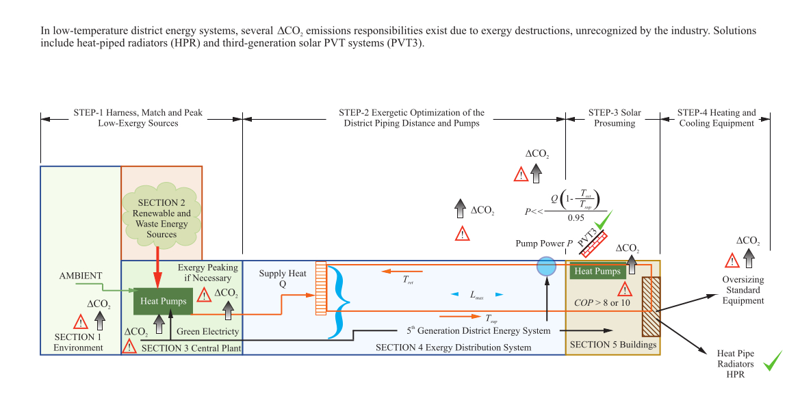
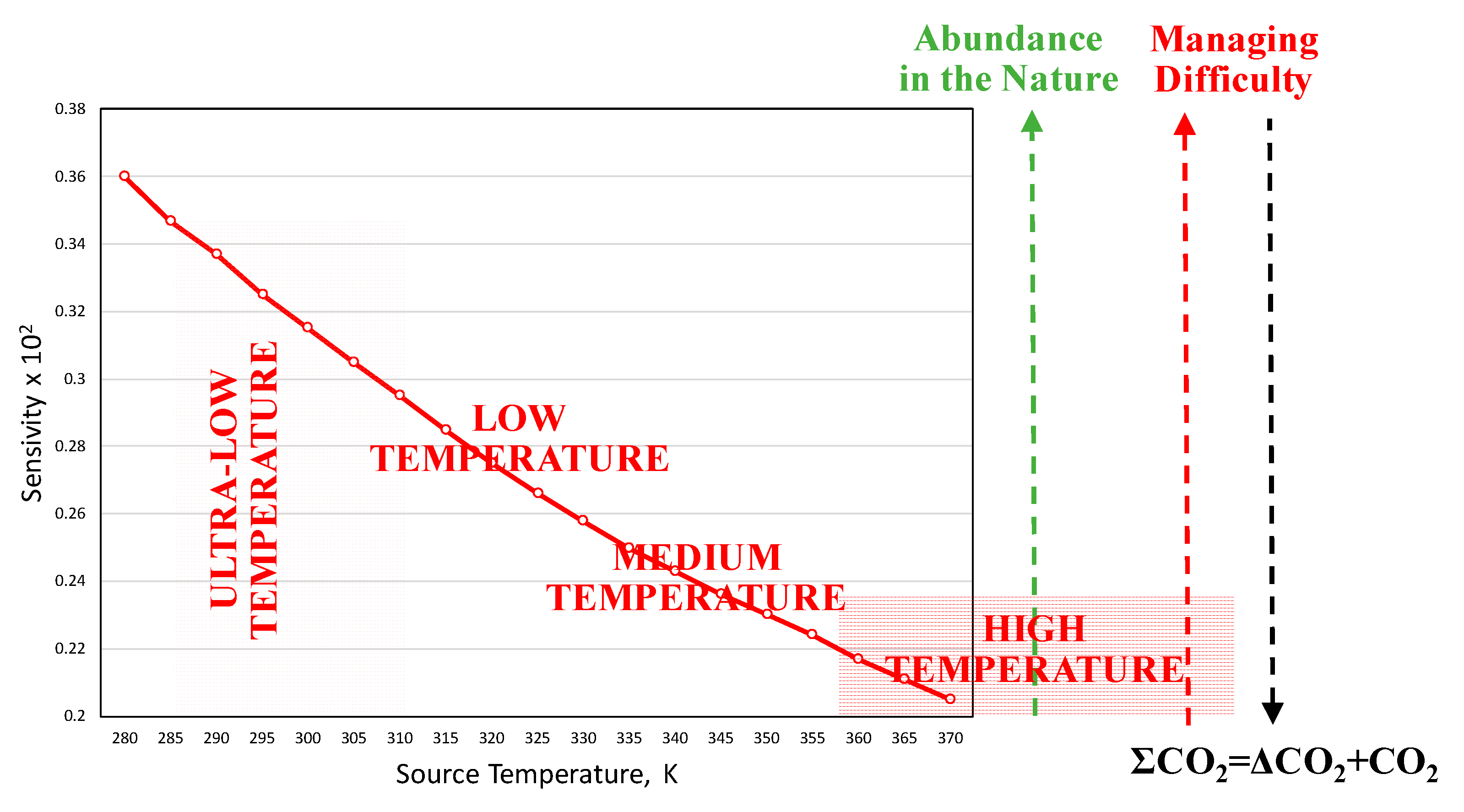
  • Decarbonizing the built environment is possible by tapping into the widely available low-temperature renewable and waste heat sources.
  • District energy systems may be helpful to achieve this goal.
  • However, low-Temperature district energy systems can be successfully applied provided that:
    (a)
    District circuit loop length is optimal concerning pumping exergy spending and thermal exergy distribution. This issue has already been answered (Refer to Reference [37])
    (b)
    The temperature difference between the supply and return piping must be small at low supply temperatures
    (c)
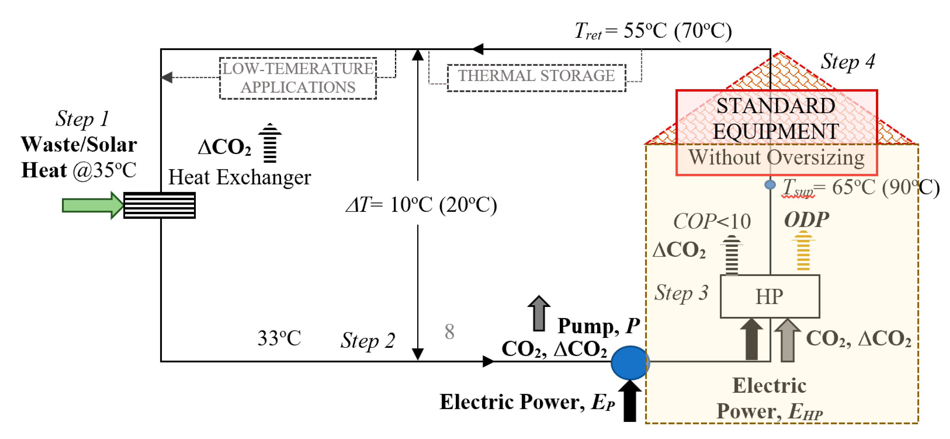
    New low-temperature heating equipment must be developed to minimize or eliminate the necessity for equipment oversizing and temperature peaking.
    (d)
    Temperature peaking with heat pumps defeats the decarbonization objective unless the COP approaches 10. Such a high value may be achieved by cascading heat pumps and de-centralizing.
    (e)
    Heat pipes, wherever they may replace pumps or fans, reduce the CO2 emissions responsibilities economically.
  • District size with the number and capacity of the interconnected solar prosuming buildings must be small due to low solar heat temperatures being shared in the circuit. In this respect, sometimes detached solar buildings may be more rational
  • Especially in low-temperature applications, exergy rationality must be prioritized.

2.1. Research Design

The main method of the research is based on the Rational Exergy Management Model (REMM) as an analytical tool to investigate the problem and verify the hypotheses. This method employs the exergy methods derived and based on the ideal Carnot efficiency and with derived metrics.
The primary research method also aims for an easy-to-comprehend algorithm of metrics and design equations that may also be understood and implemented by policymakers and comprehended by the public besides scientists and engineers. Thus, the ease of acknowledging the effect of nearly-avoidable CO2 emissions due to exergy destructions will be established and facilitated.
In this token, this research plan was based on the need for sustainable decarbonization.
Based on this need, exergy destructions, which become more dominant in low-temperature applications, like district energy systems with solar and waste heat as low as 35 °C, are linked to the nearly-avoidable (additional) CO2 emissions.
The hypotheses were verified and supported by analytical methods and derivations rather than experimentation due to the complexity and difficulties to implement the methodology to district energy systems. Mathematical tools supplemented by new verification metrics have shown that hypotheses made are accurate and correct. REMM has successfully addressed all aspects of the problem of global warming. In addition, certified tests for heat pipe radiators were conducted in line with ANSI/ASHRAE SPC 138 test chamber principles. To quantify the importance of the exergy rationality approach, three impossible cases are exemplified first.

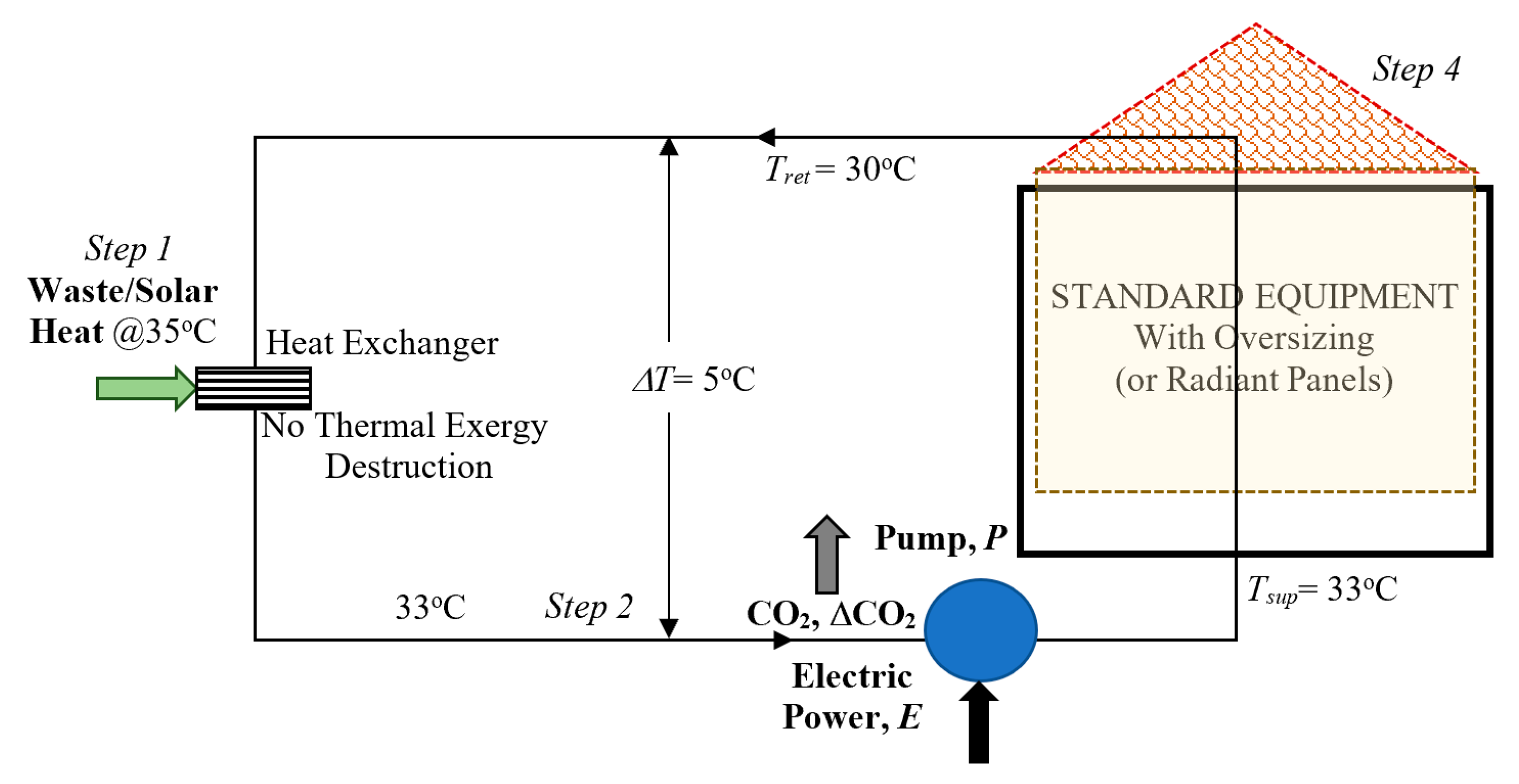
2.2. Impossible Cases with Existing Comfort Heating Equipment

2.2.1. Case 1

Figure 9 shows the basic case for utilizing low-temperature thermal sources like solar thermal or waste heat (Step 1) in a district energy system. In this case, the standard heating equipment in the buildings (Step 4) is not oversized. Instead, the district supply temperature, Tsup is peaked at the central plant by heat pumps (HP, Step 3). Temperature-peaked thermal power is distributed in the district (Step 2) by circulation pump stations, demanding a total electrical power of P. Assuming that more recent models of hydronic heating equipment are used in the buildings, such that the supply temperature is 65 °C. The return temperature is 55 °C (ΔT = 10 °C), just after one tour of thermal power distribution in the district, the waste heat or centralized solar thermal power field will become useless because the return temperature to the heat exchanger (55 °C) will be higher than the input temperature of 35 °C. This result defeats the purpose of using low-temperature thermal sources for decarbonization, while exergy destructions of the following amounts will occur, with non-zero unit exergy destructions and DCO2 amounts as shown in the following calculations These results ultimately end the operation of Case 1.
ε d e s = 1 [ ( 273.15 + 35 )   K / ( 273.15 + 55 )   K ] = 0.061   kW / kW
Δ C O 2 = 0.27 × 0.061 = 0.0165   kg   CO 2 / kW-h The   condition   worsens   for   90   ° C / 70   ° C   regime :
ε d e s = 1 [ ( 273.15 + 35 )   K / ( 273.15 + 90 )   K ] = 0.102   kW / kW   ( Δ T = 20   ° C )
Δ C O 2 = 0.27 × 0.102 = 0.0275   kg   CO 2 / kW-h
Figure 9 further shows that decarbonization goals are defeated by direct and nearly-avoidable CO2 emissions of the heat pump(s) power supply sources delivering electricity to the heat pumps and circulation pumps. Such positive exergy destructions render this application to be impossible right at the beginning of the process by not permitting the use of low-temperature thermal sources, as EU countries target for, thus also defeats the strategy of using widely available low-temperature thermal resources. In general, to make this solution workable, the return temperature must satisfy Equation (14), which shows that either equipment oversizing and or partial temperature peaking is necessary for the building.
T r e t < 35 ° C Δ T 2
There are additional constraints, such as the COP of the heat pumps will be reduced in a peaking process to higher temperatures, the district loop pipe insulation must be thicker to avoid excessive thermal losses at high supply temperatures, increased power consumption of the heat pumps leading to more CO2 emissions responsibilities as well as ozone-depleting emissions with positive ODP (Ozone-Depleting Potential) of the refrigerant). Although at a higher ΔT pumping power, demand will be smaller. Case 2 shows equipment oversizing, which eliminated temperature peaking. Electric power for the heat pump and the district loop pump(s) come with direct and nearly-avoidable CO2 emissions.

2.2.2. Case 2

This case in Figure 10 replaces central heat pumps with individual heat pumps to be installed in each building in the district. Indoor comfort heating equipment is the same without any oversizing, accommodating lower supply temperatures for given indoor heating loads. Thermal input is distributed in the district loop at about 35 °C to the buildings and then locally peaked to 65 °C by individual heat pumps to suit the existing equipment. Nothing seems to be different in terms of mission impossible, except that thermal insulation in the loop pipes may be smaller due to low temperatures at the supply branches of the district loop. Therefore, the low-temperature district energy systems may bring a new understanding to urban life and strategy to city planners by optimally using heat pumps, equipment oversizing, and additional low-temperature applications integrated into the district. Thermal storage is also an essential optimization parameter by offering peak load shaving, thus reducing peak temperature demands leading to reduction of the need for equipment oversizing.

2.2.3. Case 3

In this case (Figure 11), standard equipment is retrofitted by simply oversizing or adding more heating equipment indoors to accommodate the supply temperature at 35 °C directly without temperature peaking. In this case, however, the heating equipment oversizing ratio, F` in terms of equipment length and width product, may be seven or even more (See Section 3.1). Such an oversizing adds material weight, high cost, manufacturing embodiments, and more heat transfer fluid to the system. The latter means higher start-up pumping power requirement in on-off controls unless multi-cascade pumps are used. For single-speed pumps, this means oversizing the pump and reduced efficiency. Therefore, such a large amount of oversizing is almost impossible, especially in old buildings, to be retrofitted. In the EU countries, more than half of the buildings are older than 50 years. The only rational option is radiant panel heating systems solar PVT panels with little oversizing [38,39,40], which is also material, pumping energy-intensive, and almost impossible to retrofit the floors or ceilings in old buildings [40]. In this case, because ΔT needs to be small at such low temperatures in the entire district loop, pumping power in the district will be higher.
The above three cases show the impossibility of utilizing low-temperature thermal sources with existing heating equipment in buildings connected to the grid. The feasible resolution of the conflict between low-temperature thermal sources and high-temperature equipment lies on the demand side, namely buildings with new heating equipment, which need little or no oversizing at low supply temperatures, and without any performance compromise. One such viable solution is to use heat pipes in new equipment designs to obtain more favourable performance characteristics. In 1963, Los Alamos physicist George Grover successfully demonstrated his invention of the heat pipe. Grover’s inspiration for the heat pipe came from rudimentary heat-conducting pipes used by British bakers more than 170 years ago. A heat pipe is a heat-transfer device that combines the principles of both thermal conductivity and phase transition to transfer heat between two points at different temperatures effectively. They have very high effective thermal conductivity and provide a fast response to operational changes.

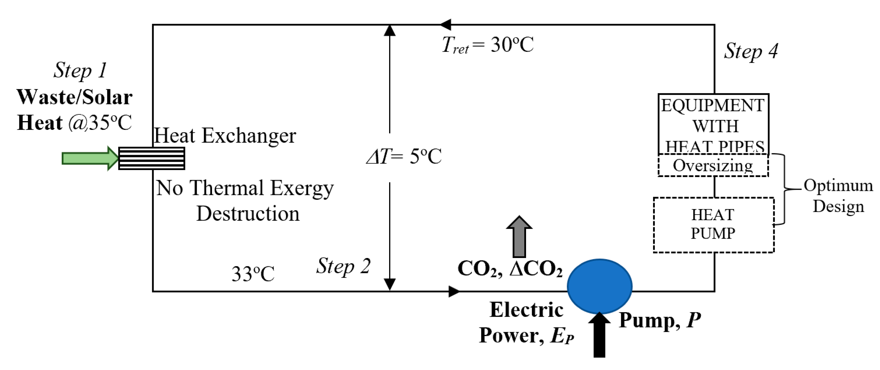
2.3. Possible Case: New Heating Equipment without or Little Support from Cascaded Heat Pumps

Case 4

In this technically and economically viable case (Figure 12), new equipment designed with heat pipes with little water content and better thermo-mechano-hydraulic properties is much lighter and requires little oversizing. If temperature peaking is necessary, heat pumps must be cascaded to improve the overall COP equal to above 10 [41]. The only remaining sustainability challenge for achieving the goals of EU for 5DE systems is the high preciseness and accuracy required to control the system at such low temperatures. The sensitivity in matching the low-quality exergy of such widely available resources with the demand is critical. This condition is depicted in Figure 13 and Equation (15). Any perturbation in the temperature affects the sensitivity of exergy in terms of ΔT by its square.
( Δ ε Δ T ) = T r e f T 2
The challenge of sensitivity-if resolved (System Management Difficulty), will pay off by the ability to utilize widely available low-temperature thermal sources for and decarbonization. Besides, less power is consumed by heat pumps (or no heat pumps: zero power), negligible ozone depletion effect due to reduced refrigerants in heat pumps, if used, minus more power demand by the district main loop pumps. Despite several advantages and potential contributions to the 5DE low-temperature and ultra-low temperature district heating and individual building heating sector, heat-pipe radiator technology is not commercially mature yet, except for some experimental studies.
Kerrighan et al. provided useful information about the advantages of the heat-pipe radiator concept following their early demonstrative tests on a bench scale with partial support from the EU and under the Ireland Grant CFTD-07-IT-307 [42]. Figure 14 shows the so-called heat-pipe natural convector.
The first commercial product, Enover Heat-Pipe Radiator (HPR) with 3-phase refrigerant-filled wickless heat pipes, EHP, is shown in Figure 15 [43]. The full-size experimental prototype is shown in Figure 15.

2.4. Models of Each Step (1 to 4)

Step 1. Supply: Central District Plant and the Next-Generation PVT Systems of the Prosumers.
Supply is both from the district central plant and the prosumers circulated on the main district loop. The primary source at the district central and prosumer scales is the solar PVT system. The thermal supply needs to be at low temperatures, which can be readily accommodated with heat pipe radiators with little oversizing and generally without temperature peaking, to maintain the rated PV efficiency with active cooling. To achieve this condition, however, the heat transfer fluid must be circulated fast, which requires more electric pump or fan power. In this respect, control caution must be paid such that the electrical power demand for the coolant circulation must be less than the total exergy supplied by PVT (Figure 16).

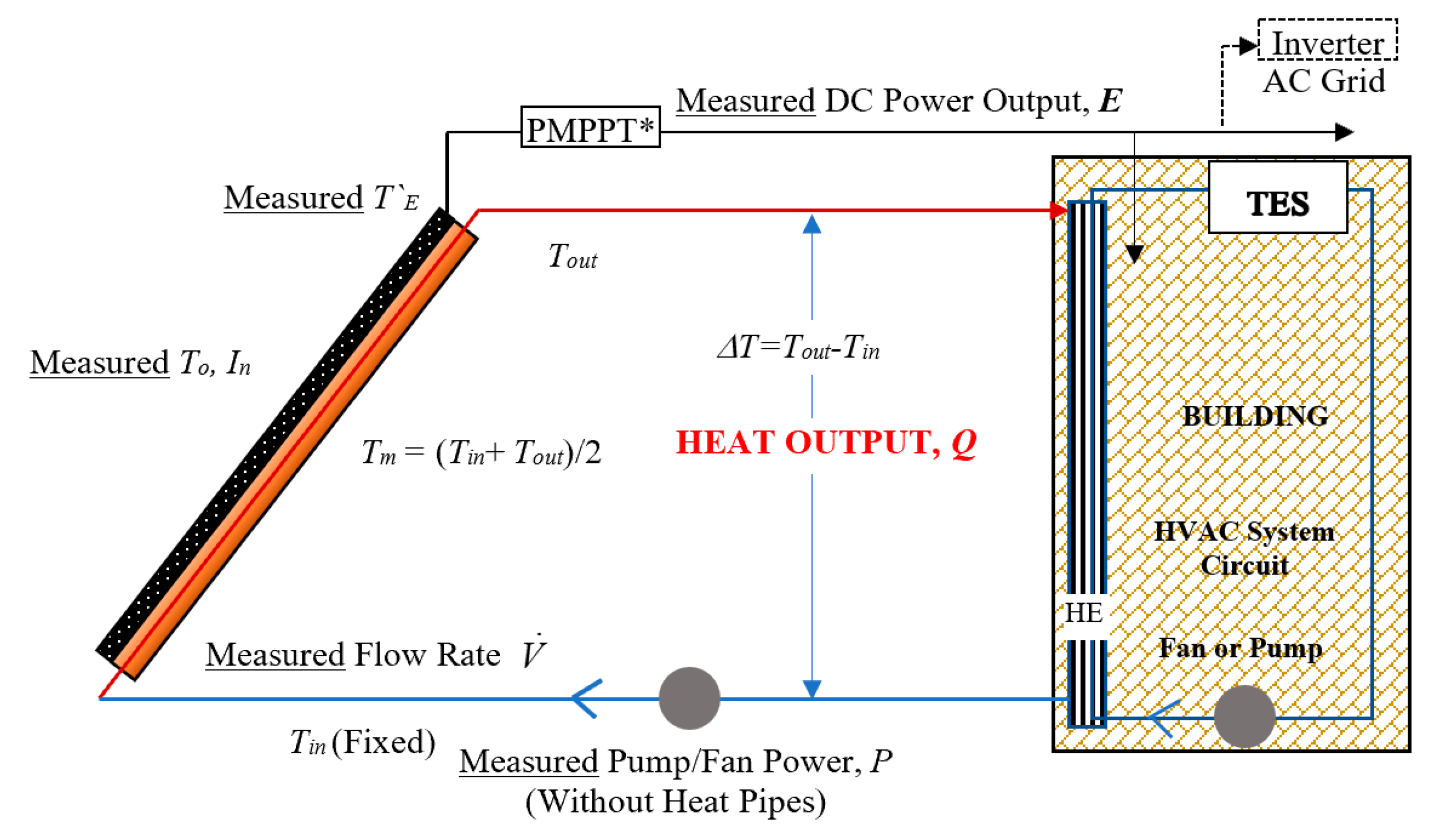
2.4.1. Optimum Pump Control in PVT Panel
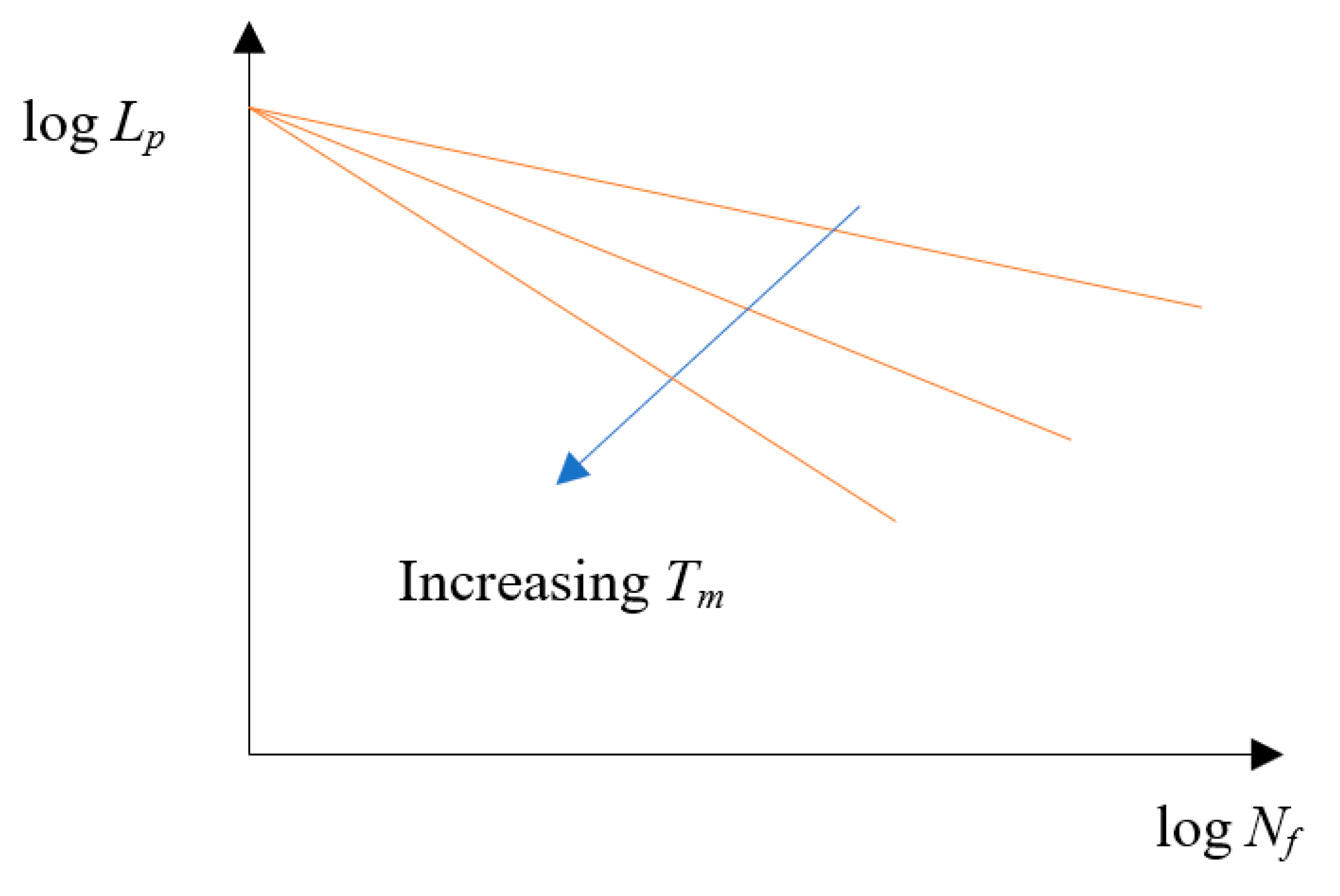
From Equation (16), Tout is solved for give solar insolation and operating conditions.
Q = I n A p η H E ( V ˙ ) = ρ ( T m ) V ˙ C p ( T m ) ( T o u t T i n )
T o u t = I n A p η H E ( V ˙ ) ρ ( T m ) V ˙ C p ( T m ) / 1000 + T i n
Equations (16)–(18) solve the optimum Tout, while TE or Tm calculates instantaneous PV efficiency with the corresponding temperature Tout. The pump selection is critical and must be dynamically controlled for net-positive exergy gain, as given in Equation (19).
T m = T o u t + T i n 2
  E X = ρ ( T m ) V ˙ C p ( T m ) ( T o u t T i n ) [ 1 T i n T o u t ] 1000 + ( I n A p ( η o { 1 β ( t m t s ) } ) f ( V ˙ ) ) [ 0.95 ] > 0 ( Exergy based )
Control for maximum ΣEX will be a simple function of the dynamically adjusted flow rate:
d   E X d V ˙ = 0 ( Maximize )   ( Energy based )
Maximum permissible pump power P, which is a function of V ˙ can be solved from the positive exergy condition in Equation (21), referring to a simple PV (No heat). This is Design Limit 1 and omits ΔCO2 (c` = 0.2 kg CO2/kW-h for natural gas).
d C O 2 = ( E ` P ) × 0.2 × P E F + Q 0.2 η b o i l e r > 0 ( Design   Limit   1 )
Equation (21) gives the implicit uncertainty in calculating the CO2 emissions according to PEF, P, Q, and boiler efficiency. PEF, which is the fuel-to-plug electricity generation and transmission (The current standard value in practice is 2.5 in the EU). First of all, there are four different methods to evaluate PEF, which ranges between 2.09 and 1.84 for 2020 (Target values). Furthermore, current methods with different uncertainties do not account for exergy destructions in the power mix and the power chain. Even further, specific values for the countries are different. Therefore, the uncertainty of dCO2 depends largely on PEF if other terms are fixed, namely:
Δ ( d C O 2 ) = c ` Δ P E F
dCO2 is also sensitive to the pump power, which is a function of the loads, Q ˙ . The boiler efficiency is also a function of the loads and the environmental conditions. E` is the ratio of the power output increase after PV cooling during positive generation of heat, Q:
E ` = E ( 1 β { T m T s } 1 β { T E ` T s } 1 ) > 0
PEF is the primary energy factor, 2.5 (Current EU Average). A second limit for the maximum permissible power, P, may be calculated from Equation (24).
P < E ` + Q η b o i l e r × P E F         ( Design   Limit   2 )
The pump capacity must not exceed Limits 1 and 2, whichever comes first. All exergy-destruction-related challenges due to pump electricity demand for thermal power generation may be eliminated by replacing the fluid circulation behind the PV panels by attaching heat pipes. Heat pipes eliminate onboard pumps or fans. This is the first major contribution of heat pipes in solar thermal systems

2.4.2. PV Life

As important as maintaining the PV efficiency, PV material fatigue due to temperature cycles during day and night and on-off periods, especially in mountainous and hot climates, is essential, especially if an active cooling system is not present. The physical life of the PV cells, Lp (years), decreases in a logarithmic fashion, depending upon the cumulative number, Nf and the average magnitude of the temperature swings as a function of Tm, as shown in Figure 17.
Figure 18 shows an advanced, pumpless PVT system with heat pipes and embedded thermal storage [44]. The second and the third contribution of heat pipes for the next-generation district energy systems with solar prosumers will be a heat-pipe radiator (HPR) [43], and the on-site thermal storage, all of which operate at low temperatures already and are equipped with heat pipes.
Another option on the central plant scale is a renewable-energy hybrid cogeneration system. Figure 19 shows a novel arrangement where the PVT units are mounted on swivels attached to wind turbine towers. PVT panels have one axis of freedom such that when combined with swiveling action, PVT gains a good sun-tracking ability. PVT systems have heat pipes to deliver low-temperature heat to the district. PVT panels have embodied heat pipes to claim heat from the PV panels and therefore do not demand pumping power. Heat is delivered to a header system in the tower, which transmits the thermal power to the district with the district pumping system. Surplus electrical energy is stored in the tower as compressed air, which is returned to electric power when need by using an air-powered turbine.
Step 2. District Energy System with Solar Prosumers.
The size of the district thermal loop that interconnects presuming solar and greens buildings is very important. The holistic model addresses the maximum allowable one-way district piping distance, namely Lmax, by comparing the exergy of the thermal power, namely Q ˙ D , which is shared among the prosumers and the central district plant by the district consuming exergy for district pumping, PE [37]. The following formulations show that Lmax must be determined first from the 2nd Law [37].
L m a x ( 0.273 79 T D S ) × ( η P η m ) w × Q ˙ D 1.5 32 0.95 5 π ρ C p [ 0.273   T D S 79 ]       ( In   district   heating   and   T D S > T r e f ,   Exergy based )
L m a x | 0.4 + 120.2   K T D S | × ( η P η m ) w × Q ˙ D 1.5 32 0.95 5 π ρ C p | 0.4 T D S 120.2   K |           ( In   district   cooling ,   Exergy based )
If the average number of floors in prosumers, n increases, the total piping length decreases but the thermal energy transfer in the pipes increases, and solar insolation area per building floor decreases with n. A direct relationship between the pumping power per piping length and the average number of floors has been developed. In Equation (27), y and p are the constants depending on the district characteristics and size, climate, and building typology.
P E L y n p
After letting L = Lmax and then solving related equations simultaneously, the following expression for the maximum allowable total pumping power, namely PEmax, is obtained.
P E m a x y × L m a x n p
For city planners and architects, these equations allow them to optimize n, L, and PE for minimum total CO2 emissions, including avoidable emissions during the operation of the district energy system:
  C O 2 = C O 2 + Δ C O 2 = ( c ` × P E F ) P E m a x ( 2 ψ ¯ R ) ( c ` × P E F ) y × L m a x n l ( 2 ψ ¯ R )                 ( Exergy based )
Equation (29) introduces the variable, ψ ¯ R , again, which must be maximized by designing and implementing exergy rational power supply, distribution, utilization technologies, and suitable buildings for 5DE systems by minimizing exergy destructions. Solar cogeneration (PVT) systems have low exergy destructions, and they are vital assets in this respect. Furthermore, Lmax expressions and imposed ΔT limitations provide helpful information in selecting the supply and return temperatures at optimum flow rates. Equation (29) also shows that ΣCO2 is a linear function of the circuit length. It may be presumed that by using multiple circuits in (nn) number of shorter identical district lengths, Li emissions may be reduced while pressure head is also reduced. This condition is possible only if Equation (30) is satisfied, which brings another optimization dimension by an optimum number of parallel circuits. The term h is the pump head for a single loop pipe length of L.
( h n n ) i = 1 n n L i < h L
Assuming a linear relation between ΔT and TDS, the maximum allowable district distance from the plant also decreases. Therefore, 5DE systems must be shorter in heating because they rely on ultra-low temperatures. For example, Lmax decreases by 1/1.54 when TDS decreases from 345 K to 308 K. In cooling, Lmax must also be shorter at higher supply temperatures. This condition is a trade-off between utilizing low exergy thermal sources and more infrastructural embodiments. There is a definite relationship between the average number of floors, n and the pay-back period, Y(n):
Y ( n ) = C n [ l ( m p 2 + 1 ) k ]
The coefficient mp represents the effect of the pipe wall thickness on its pressure resistance according to diameter. Terms C, l, and k depend on the specifics of a district energy system. Then, Equation (31) deduces the economics of the district energy system size, i.e., decentralization versus centralization.
  • If ( m p 2 + 1 ) k > 0, then the pay-back period increases with n,
  • If ( m p 2 + 1 ) k = 0, then the pay-back period is independent of n,
  • If ( m p 2 + 1 ) k < 0, then the pay-back period decreases with n.
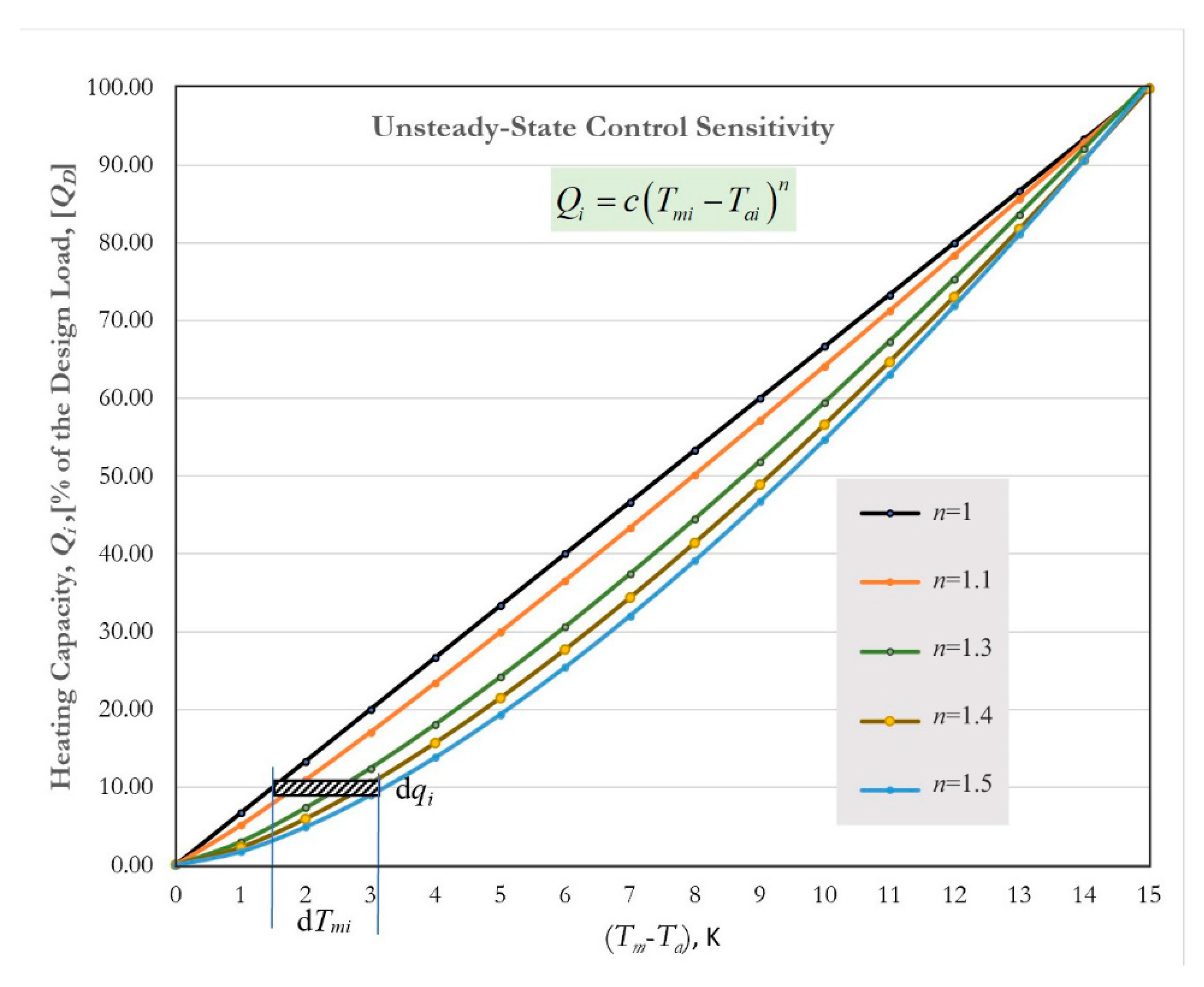
Generally, case (a) applies, meaning that high-rise buildings must be avoided with less solar insolation surface area per floor to prosume. Simply put, city planners are faced with a highly complex problem about deciding the average number of floors in the buildings of a city.
Step 3. Optimum Equipment Oversizing Versus Heat Pumps.
Equipment Oversizing for Temperature Drift from To prosumer TUL: When the supply temperature is less than the design value of given indoor heating equipment, then the equipment capacity decreases. To recover the design heating capacity, the equipment needs to be oversized. Figure 20 compares the oversizing issue about a standard radiator and a heat pipe radiator, without any external temperature peaking like a heat pump. Equation (32) gives the oversizing formula, which also considers exergy loss in a standard radiator, while it only approaches the design capacity asymptotically. According to Figure 20, T4 is the effective temperature at the final oversizing step (i = 4). Exergy Penalty Factor represents the thermal exergy drift from TUL to T4. The exponent (n) is an equipment characteristic [12]. For radiant floor panels, (n) is 1.1. For standard radiators, it is 1.33. For fan-coils, it is 1.4 up to 1.5. The second additive exponent (m) is a new coefficient, which has been derived to represent the diminishing oversizing effect (Figure 20). Dry-Bulb (DB) indoor air temperature and Area-Averaged Unheated Surface Temperature (AUST) are assumed to be equal and constant in all steps.
F ` = ( ( T o T a ) ( T E T a ) ) n + m / ( T 4 T U L )   ( Exergy   Penalty   Factor )   ( Energy-based )
where
  • n—Capacity Factor
  • m—Temperature Drift Factor
Example 1. 
For SR, n = 1.33, m = 0.2, Tm = 65 °C, Ta = 20 °C, TE = TUL = 32.5 °C, T4 = 25 °C.
F ` = ( ( 65 20 ) ( 32.5 20 ) ) 1.53 / ( 25 + 273.15 32.5 + 273.15 ) = 7.098 / 0.975 = 7.28
Such an oversizing capacity is technically impossible.
For HPR, n = 1.1, m = −0.25, Tm = 65 °C, Ta = 20 °C, TE = T4 = TUL = 32.5 °C.
F ` = ( ( 65 20 ) ( 32.5 20 ) ) 0.85 / ( 32.5 + 273.15 32.5 + 273.15 ) = 2.97
This example shows that heat pipe radiators require almost 60% less oversizing, which means savings in indoor space, weight, embodiments of material, less CO2 emissions responsibility, and pumping requirement. It may be concluded that heat pipe technology is technically, environmentally, and economically feasible and applicable as a retrofit tool, including old buildings. For HPR, the exponent (m) is less than zero because heat pipe performance usually overshoots while it is customizable to adapt for low mean supply temperatures, ability to employ thinner heat pipe thickness by reducing the heat pipe pressure, and smaller heat pipe diameter for better fin performance. A negative m value represents this overshooting. There is only one oversizing step instead of oversizing cascades in a standard radiator. A standard radiator (SR) in Figure 20 undershoots the target capacity, Q in every oversizing cascade, and requires further oversizing steps in a diminishing return until the limit of laminar flow is reached because the fluid flow in each parallel heat transfer pipe decreases with oversizing.
V k = V o F k `             ( SR   Only )
F k ` = i = 1 k F i `           ( SR   Only )
Equations (33) and (34) apply only to SR-type radiators. Unless the ΔT between supply and return temperatures is decreased accordingly, increasing the pumping power exergy demand, the original heating capacity may not be reached. To minimize the loss in the capacity, ε, the regular oversizing factor is modified by the temperature drift factor m, which is greater than zero.

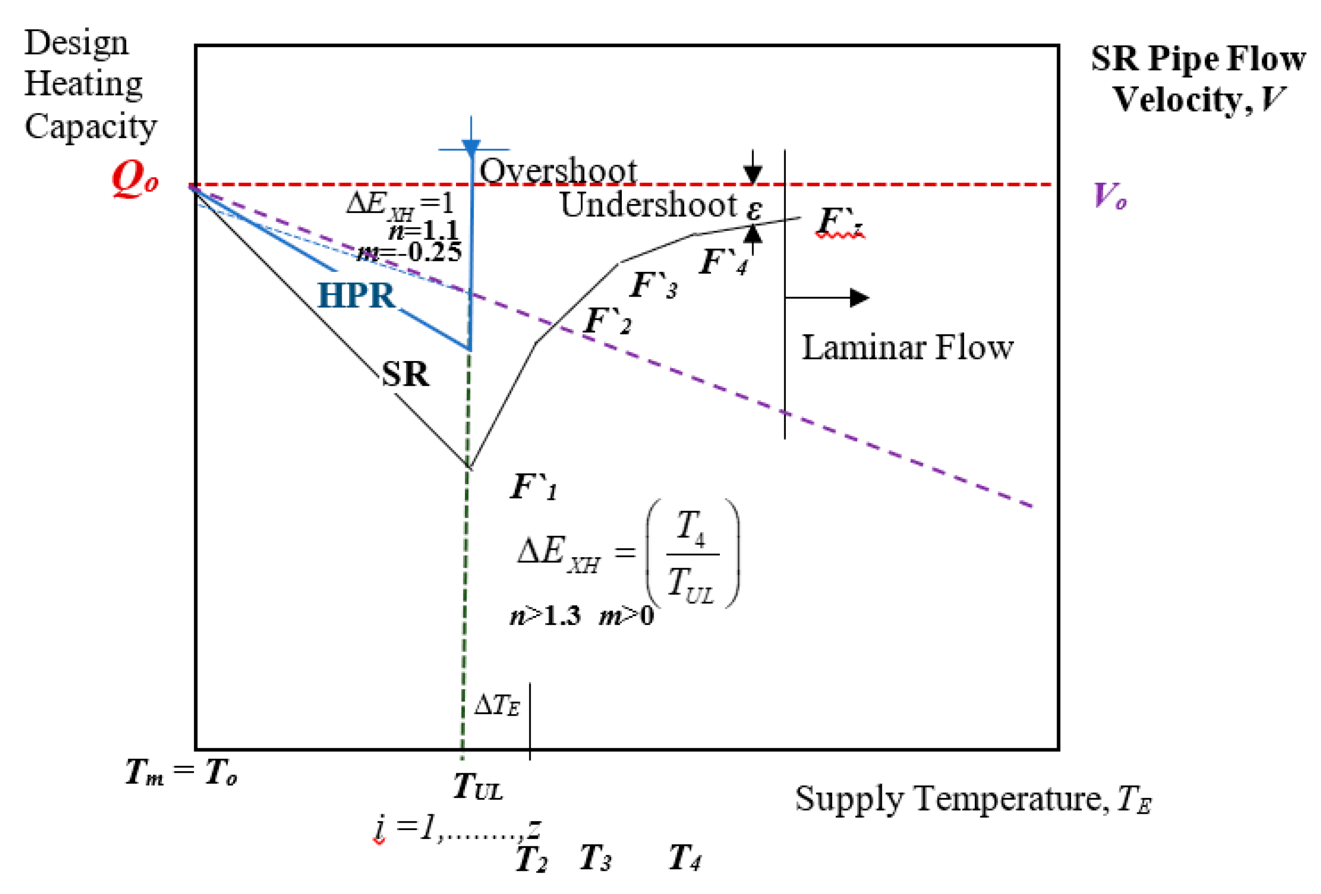
2.4.3. Solutions for Figure 20

Conventional (Standard) Finned Panel Radiator (SR):
A typical conventional (standard) finned panel radiator (SR) with heat transfer fluid circulating in vertical pipes is shown in cross-sectional view as shown in Figure 21. Forced convection heat transfer coefficient, hs between the fluid and the pipe’s inner wall decreases with oversizing. This negatively affects the overall performance of the radiator. Once the radiator is oversized by adding more tubes sidewise in the same proportion of oversizing, F`, each tube receives a smaller heat load in an inverse proportion of F`. The average fluid velocity, V, in each tube also decreases with F`. These affect the heat transfer convection coefficient, hs between the fluid and the inner pipe surface. hs is a function of the fluid Reynolds Number raised to the power 0.8. Thus, it is a function of V0.8, provided that all other variables and fluid properties are fixed. The original design value of V before oversizing is equal to Vo. Figure 22 shows the simple thermal resistance diagram.
r s = 1 h s D i = 1 c ` ` ( V o F ` ) 0.8 D i = F ` 0.8 c ` ` `
q e q 4 σ ε T e q 3 ( T p T a ) + 5   W / ( m 2 K ) 5 × 10 8 T e q 3 ( T p T a ) + 5   W / ( m 2 K )
T e q = T p + T a 2
qeq is the combined heat transfer flux due to surface radiation observing AUST (assumed to be equal to Ta), and the surface natural convection observing Dry-Bulb (DB) indoor air temperature Ta. TE changes with oversizing of standard radiators, as shown in Figure 20. Tp is assumed to be uniform across the front panel of the radiator (ideal fin efficiency). The term req was defined for a panel area of Moc × 1 m of tube height. The thermal resistance of the tube wall is neglected [40]. rf may be derived from the literature [45].
r e q = ( T p T a ) M o c q e q
For the Configuration in Figure 20,
rc = 0.38 MOC (m2K/W)
rp = tp/kp
The simple oversizing factor is calculated from the following equation (m = 0):
F ` = ( T m T a T E T a ) n           ( Equipment   Oversizing )
( Q o F ` ) = 1 r T ( T E T a ) = 1 [ F ` 0.8 c ` ` ` ] + r x ( T E T a )         ( Heat   transfer   side )
Solving for the following steps of oversizing with ΔTEi+1:
Δ T E i + 1 = Q o { [ 1 F i + 1 ` ( ( F i + 1 ` ) 0.8 c ` ` ` + r x ) ] 1 F i ` ( ( F i ` ) 0.8 c ` ` ` + r x ) }
From the general equation of equipment performance capacity,
Q = c o ( T E T a ) n         ( Thermal   Performance   Side )
Δ Q i + 2 = c o n ( T E T a ) n 1 Δ T E i + 1
The next oversizing step must compensate for the undershooting amount of capacity, ΔQi+2, after returning (z) times to Equation (32), which accumulates the oversizing value to ƩF`z until the solution converges to an error function, ε or meets the laminar flow limit, whichever comes first. A simple computer program solves (m) by comparing the overall oversizing factor to the original one at step 1. The computer program further refines (m) iteratively by replacing (n) with (n + m) in each repetitive run of the nested loop in the computer program until the solution finally converges for (m).
m = ln   F z ` ln   F 1 `
Heat Pipe Radiator: As an additional attribute of HPR, depending on the design supply temperature, TUL, the content composition, and gas pressure along with different wick constructions, and even the heat pipe diameter and its wall thickness may be better optimized with less critical strength limitations to increase the overall heat transfer rate from the radiator, such that this customizable feature may lead to a negative m value. For example, at 65 °C (Design Supply Temperature), a patented 3-phase heat pipe (EHP) fill reaches a pressure of 12 bar [41]. The same heat pipe filling during operation at 35 °C stays at 6 bars at a concentration of 0.4758 g/m3. EHP does not require external power to actuate the nanoparticles. In other words, the lower the supply temperature, the lower is the pressure. This relationship lets the designer better deal with the hoop and axial stresses, such that the pipe wall thickness may be reduced, which further reduces the radiator weight, embodiments, cost, and at the same time, increases the surface temperatures for a higher convection coefficient. Pipe diameter may increase to maximum fin efficiency, better contacts, thus higher radiation, and convection coefficients. Despite these advantages, the heat pipe’s effective thermal conductance may decrease, affecting the response time for fluctuating thermal loads in the indoor space. Therefore, a supply temperature-responsive design is possible with m ≤ 0. This feature is not available for radiators without heat pipes. Figure 23 compares the hydrodynamics of SR and HPR. An HPR type of heating equipment has a material weight advantage by a factor of more than two for the same heating capacity. On the other hand, water content density per oversizing, F`/WW is negative for an HPR radiator, concerning a reference of 1 kg of water fill per kW heating capacity:
W D = F ` W w 1         ( Metric )
Optimum Supply Temperature
For the fifth generation and the beyond (5DE+) district energy systems, the supply temperature may be around 313 K (40 °C) or even less. If the transition of the standard heating equipment is possible only by oversizing them like adding more radiator sections or adding more radiator units, mostly in series in the latter case, which applies for many moderately old buildings, then pressure heads do increase. This increase is coupled with higher pumping power at the start-ups in an on-off type of controls facing larger volumes of heat transfer fluid accelerated in the entire system due to oversizing. These disadvantages may be offset by installing larger-diameter pipes, but this is quite unpractical in the existing building stock, which also adds embodied cost, energy, and CO2 emissions. New heating equipment with heat pipe technology may play an important role in overcoming such problems. For example, new radiator designs with 3-phase heat pipe technology, which is symbolized in Figure 23 [41], contain a minimal amount of heat transfer liquid, only in the hydronic supply pipe at the bottom, which is slightly larger in diameter, D when compared to standard radiators (SR). Heat is transferred and distributed to the radiator by heat pipes instead of water tubes. The exponent (n) is 1.1, which makes the temperature control more manageable and more responsive, while it also helps reduce the need for oversizing the units with a negative (m) value in many cases in practice.
Q = c ( T s u p T a ) n F `
In the cooling mode, chilled beams and hybrid wall heating and cooling panels have similar advantages in utilizing high-temperature wastes or heat pump outputs, which improve the COP of heat pumps in the cooling mode. 3-D printed composite-integrated radiators may also be possible, replacing Aluminium material from the stock, which has more embodiments. However, the flammability of certain composites needs to be considered. However, 5DE systems between 35 °C to 45 °C offer an advantage for thermal durability. Fire retarding organic material may also be used [37].
Economic Optimization
An optimum point exists between the heat pump and or equipment oversizing, Tfopt (Point C in Figure 24):
T f o p t = C e q C 2 C h p / C 1 + T a ( Without   Auxiliary   Temperature   Peaking )
If there is a temperature deficit between the optimum Tf1 for the heat pump and Tf2 for the equipment, the temperature may be further peaked by an amount dTt using an auxiliary heater, requiring an additional LCC factor, Ct.
Equation (51) solves Tf2opt and satisfies Equation (53).
d T t = T f 2 T f 1
T f 2 o p t T f e q + ( C t C 1 C h p ) = 0
C o t = C t d T ( T f e q T f 2 )
C e q C 2 ( T f 2 o p t T a ) 2 + C t [ 1 ( T f e q T f 2 o p t ) ( T f 2 o p t T f 1 o p t ) ( T f e q T f 2 o p t ) 2 ] = 0
Optimum Cascading of Heat Pumps
Figure 25 compares a one-step temperature-lift heat pump with (NHP) number of tandem heat pumps with equal temperature lifts. For a high-performance heat pump, typical q and r values may be 5 and 0.04 K−1, respectively. Then Figure 26 gives an example with two tandem heat pumps (NHP = 2) [39]. At the break-even point of net exergy gain, each heat pump needs to have at least a COP value of 3.45.
Δ T o = T s u p 2 T s u p
Δ T i = ( Δ T o N H P ) = constant
C O P i = q ( r Δ T i ) = q r ( Δ T o N H P )
Therefore, tandem heat pumps only save exergy and reduce direct CO2 emissions in terms of a given mix of the unit CO2 content of fuels for power generation corresponding to a specific country, c`. A typical c` value is 0.26 and 0.53 is a given value for ηpp. At the break-even point, both exergy and energy gains are zero, yet less power is on-demand while more low-exergy resources are demanded.
C O 2 s a v i n g s = c ` η p p ( 1 C O P 1 1 C O P 2 )                     ( Maximize )
If low-exergy sources are not abundant, the following modification is required: for heat deficit, ΔH.
C O 2 s a v i n g s = c ` η p p ( 1 C O P 1 1 C O P 2 ) 0.26 η b o i l e r Δ H
For the given break-even COPBE in Figure 26, a cheaper and simpler heat pump with a single-stage compressor with q = 4 and r = 0.1 K−1 may satisfy the COP = 3.45 condition with ΔT = 5 K. Therefore, such an exergy rationality analysis also reveals cheaper investments with the constraint on COPi.
C O P i m i n = 0.95 ( 1 T o T f ) 1
Step 4. Low-Exergy Buildings.
In the final step of the model, assuming that optimum oversizing of equipment with existing or new technology has been fixed in Step 3, with or without heat pumps, two main remaining issues are considered. The first issue is the necessity of reducing the heat loads and the second issue is the control of the oversized or new equipment with different (c) and (n) values.
Over Insulation and COP
Additional thermal insulation of the building envelope may have an unrecognized attribute, which concerns the improvement of heat pump COP according to Equation (4), given in the earlier section of this paper. If the overall heat load coefficient of the building envelope, U` is decreased by some degree of over insulation, probably above the known economic limits for investment, the equipment supply temperature is decreased; thus, COP is increased if a temperature-peaking heat pump is needed. Equation (60) gives the new optimality condition for over insulation. Here, the term tins is the COP-optimized insulation thickness after over insulation. An increase of the COP means utilizing more renewable energy sources at low temperatures at the expense of more insulation investment versus revenues from investing in smaller-capacity heat pumps and less operating costs.
t i n s = U ` ( T a T o ) | 1 T o T a | d { | 8 C O P q | + ( T s u p T a ) } n | 1 T o T s u p |
Control Issues
Figure 27 shows the performance of heating equipment in terms of different (n) values at partial loads. Any incremental change in the heat load, dQi, most probably as a result of abrupt changes in the outdoor conditions, especially if the building is not insulated, must be responded to by modulating the mean temperature of the heat transfer fluid passing through the known equipment by an amount, dTmi at the indoor DB temperature Tai at an instant (i). Taking the derivative of Equation (61), concerning Qi:
Q i = c ( T m i T a i ) n
T m i = 1 c Q i ( 1 / n ) + T a i
d T m i d Q i = ( 1 c n ) Q i ( 1 n 1 ) ,   therefore :
Δ T m i ( Q i ) = ( 1 c n ) Q i ( 1 n 1 ) Δ Q i
If n is equal to one, then ΔTm becomes independent of the absolute value of the existing heat load, Qi, when there occurs an incremental change in the load, ΔQi. Therefore, the response will be linear and independent of Qi.
Δ T m = ( 1 c n ) Δ Q i
Otherwise, starting from a cold start, while the heating load, Qi approaches 100% of the design load (increasing order), for reaching the steady-state comfort regime, increasingly more precise temperature control of ΔTmi is required (control difficulty) to respond to heat load perturbations. This is the period, which also requires a steady increase of the indoor air temperature, Tai to reach its design value. However, it is counteracted by the proportionately increasing heat losses to the outdoors, momentarily forcing Tai to stall or even drop, which is another control input. This issue becomes more critical when equipment with higher n values is present. The above discussion may also be interpreted so that the transient time for reaching the steady-state conditions with equipment having a higher exponent (n) will be longer.
For the same design thermal capacity, Q, and the same design ΔTmD of two different equipment with two different ci and ni values, the following relationship was derived:
( c 1 c 2 ) = Δ T m D ( n 2 n 1 )
After indexing c1 to the ideal condition of one, the necessary cj for a given exponent nj, which is different from one, may be expressed in terms of ΔTmD:
c j = c 1 Δ T m D ( 1 n j )
Referring to Figure 27, additional energy requirement from the source during the period between the cold start and the steady-state regime (0 ≤ Qi ≤ 100%) takes place for equipment (j) with (nj) greater than one. This difference is represented by integrating the incremental difference represented by the dTmi × dqi infinitesimal element.
Δ E j = G [ n j + 1 2 c j Q D ( 1 / n j + 1 ) 1 c 1 Q 2 ]
Equation (68) shows that exponents (n) greater than one lead to more energy consumption if an on-off type control is used. Note that if (n) is equal to one, then ΔEj is zero, and cj equals c1.

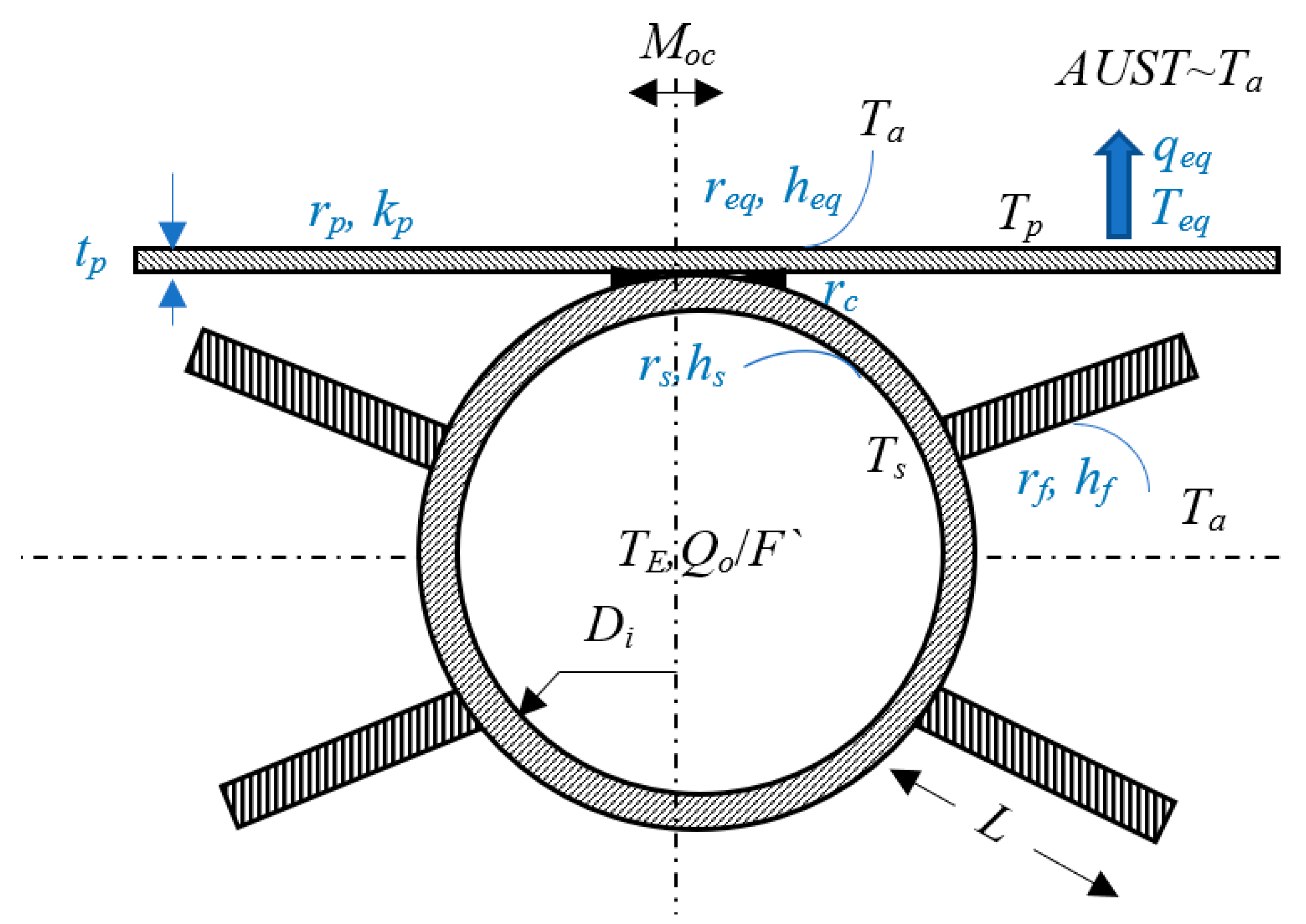
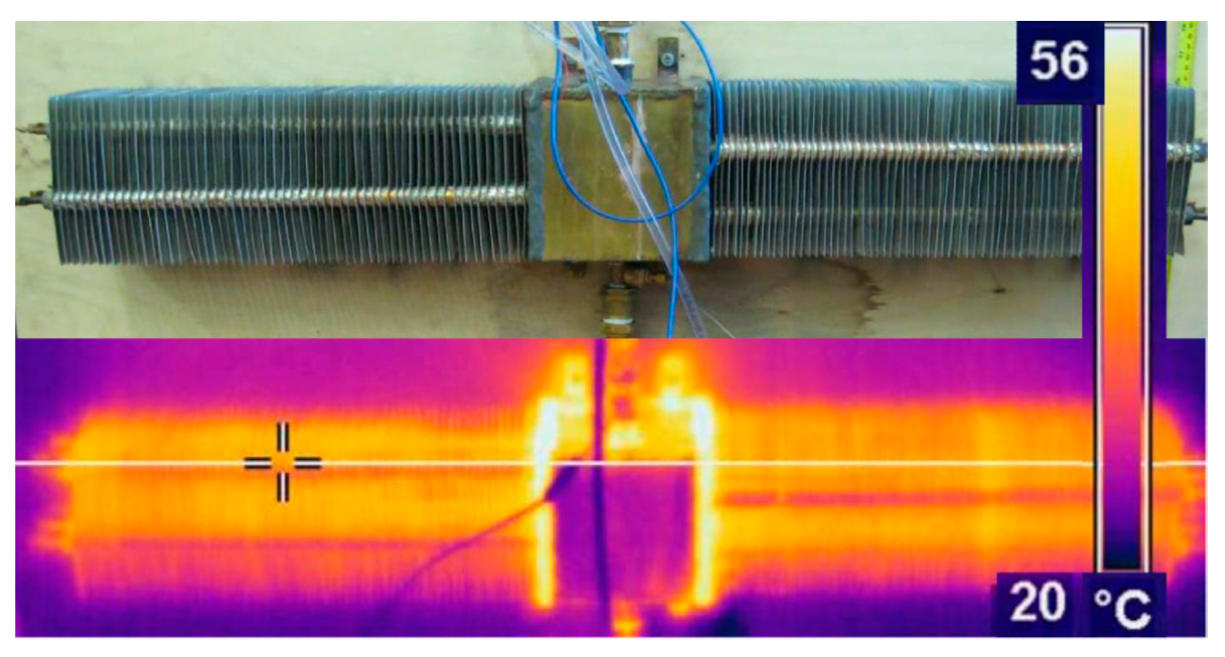
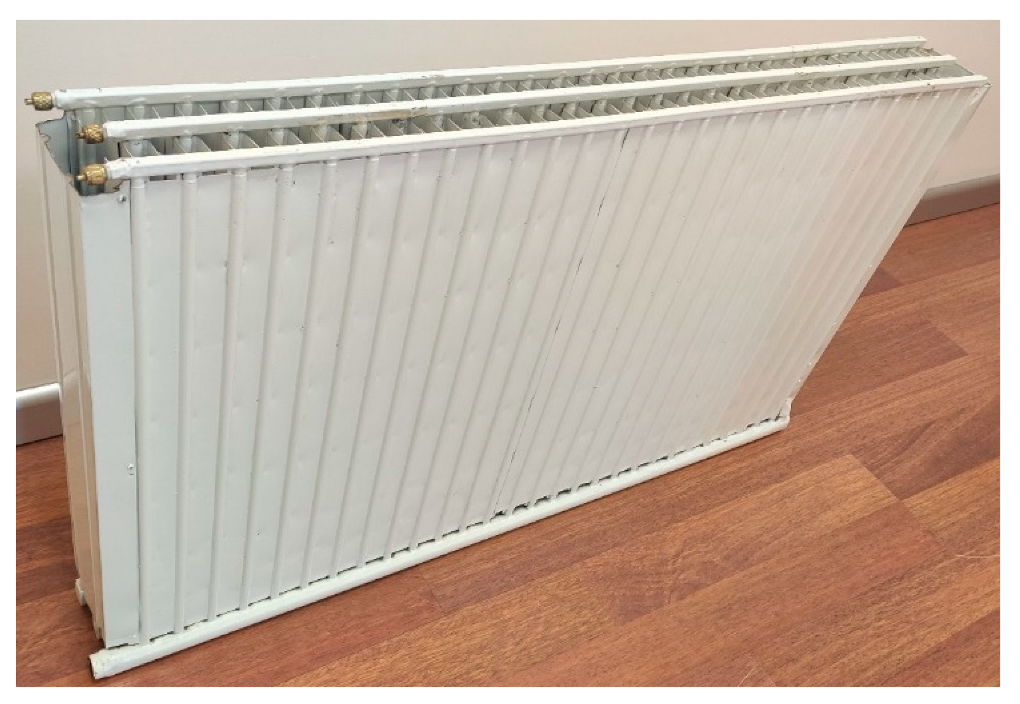
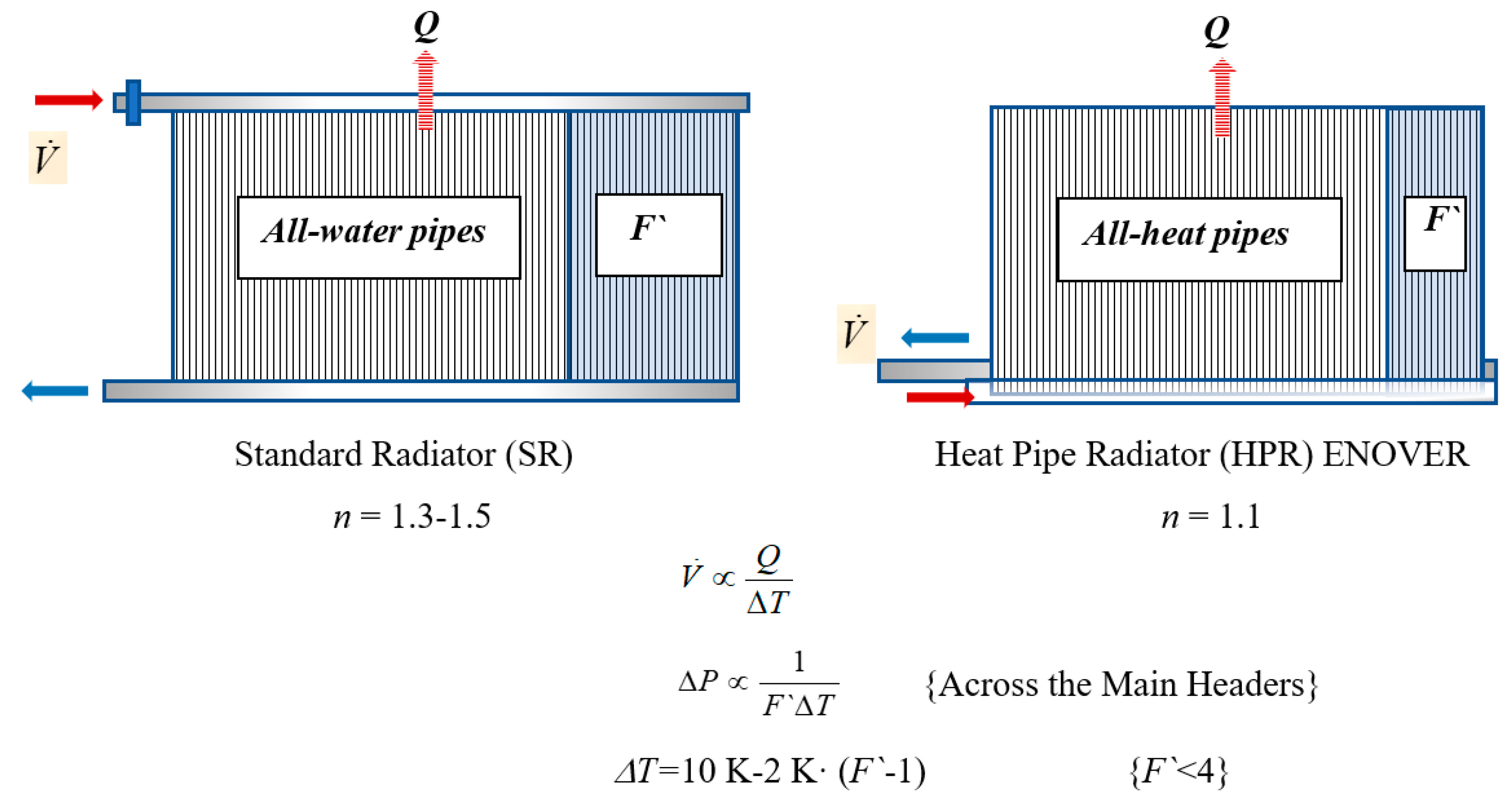
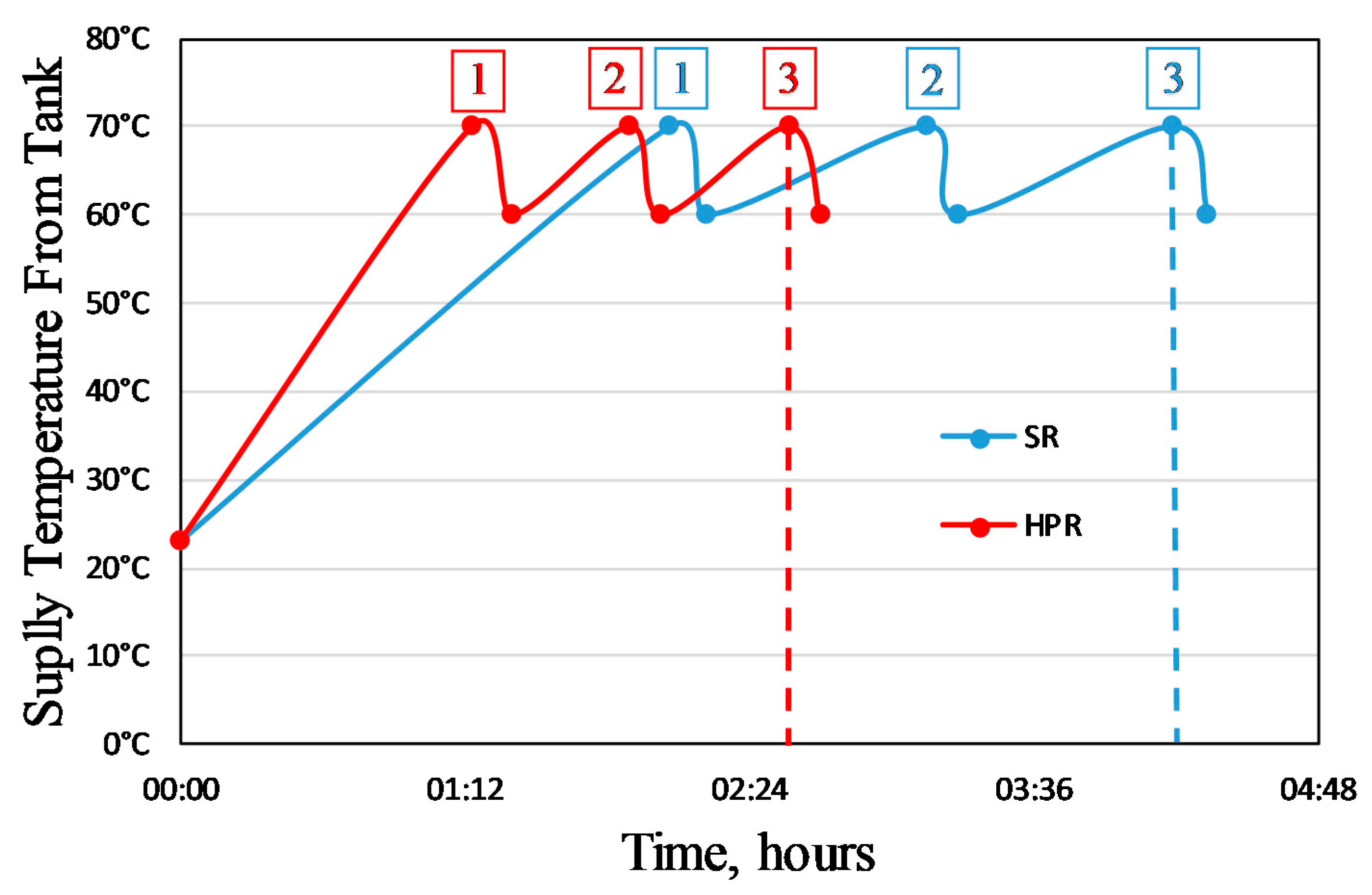
3. Analysis of Heat Pipe Radiator

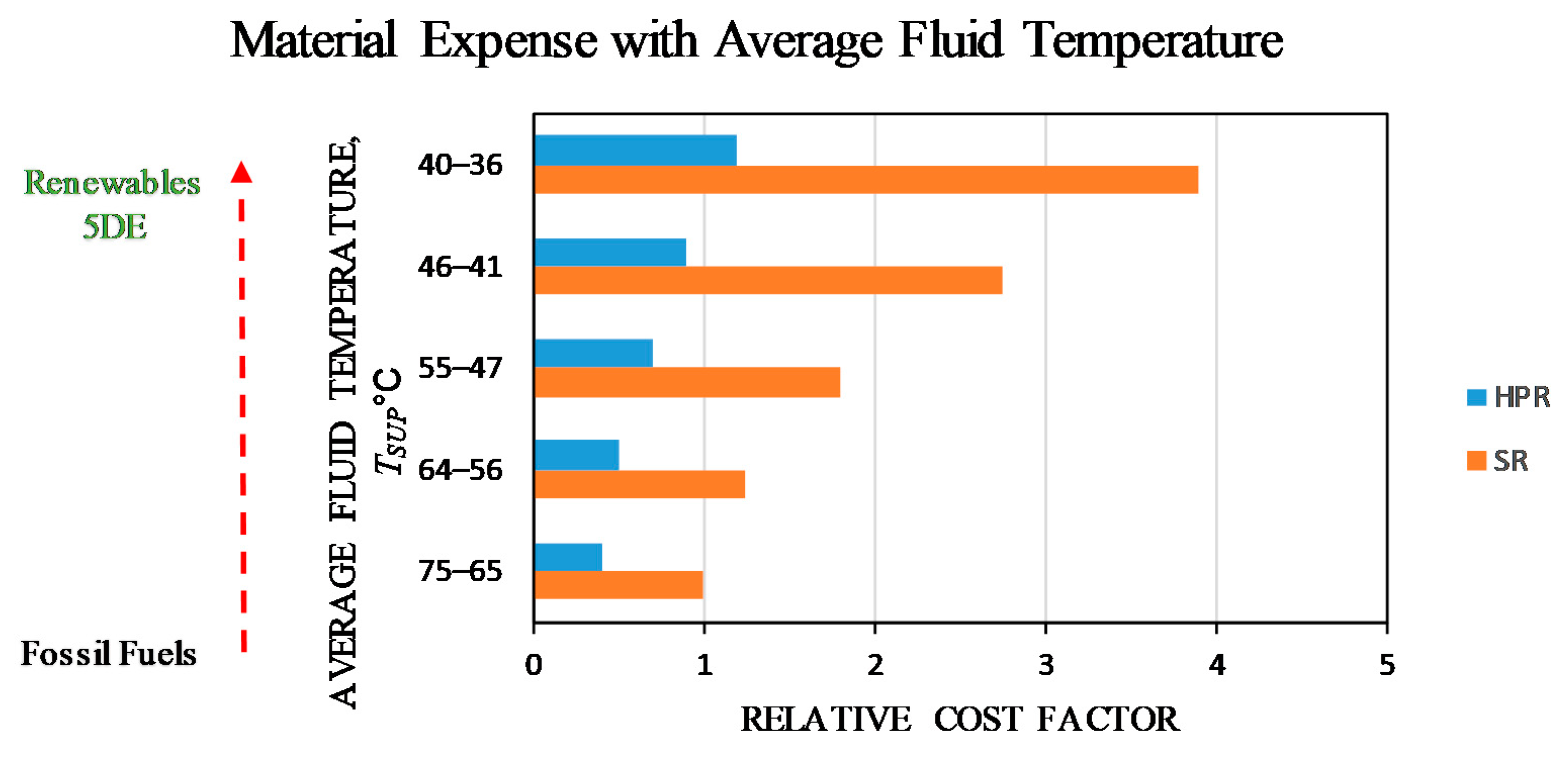
3.1. Comparison with Standard Radiator

Figure 28 compares the material expenses for SR and HPR type of radiators with oversizing effect included, as a function of the average fluid temperature ranges circulating through these sample radiators, in terms of a relative cost factor showing the cost ratio. During the transitioning process from fossil fuels to 5DE low-temperature district energy systems or prosumers, using renewable and waste energy sources, the benefits of heat pipe technology become apparent. For example, for a supply temperature range between 40 °C and 36 °C, the cost factor for SR is almost four times higher.
Table 1 shows that the overall thermal conductance of the 3-phase, wickless Enover heat pipe with the mean temperature and the position (Vertical or horizontal) does not change much. Data for the horizontal position is important for ceiling applications.
The weight difference between SR and HPR radiators in this comparison is 132.411 kg. This shows that SR systems cannot retrofit 5DE districts. On a steel material basis, the corresponding embodied CO2 is 1.8 kg CO2/kg material. An additional ΔCO2 term, 0.8, is not accounted for in the standard embodiments table (Based on the 1st Law only). On a single radiator basis: 132.411 × 1.8 = 238.4 kg CO2 embodied per radiator. In an apartment with 100 identical radiators, this is 23.8 tons of CO2.
Figure 29 is a sample plot of average CO2 savings, including DCO2 due to exergy destructions concerning pumping power required by HPR (heating capacities adjusted) compared to SR, as a function of Tm. At lower temperatures, an SR type of radiator needs more lateral oversizing, which sharply reduces pumping power demand due to more parallel pipes in the row such that each pipe receives a smaller flow. However, DT needs to be decreased to accommodate low Tm (See Figure 23), while pumping power need for HPR increases slowly.
Another important point is the thermal response time during on-off cycles. SR systems contain more heat transfer fluid than HPR systems, which have only heat transfer fluid in their supply and return headers. For example, a typical SR measuring 600 mm × 1000 mm contains 5.8 L of heat transfer fluid. A typical HPR system (Enover) contains only 0.46 L. At different flow rates corresponding to different ΔT values as a function of Tav, it takes different time intervals, tSR, and tHPR to replace the radiator contents with the heated fluid supplied by the boiler through on-off pumps, driven by indoor comfort thermostats. Figure 30 shows the tSR and tHPR values at different Tav values.
This figure shows that for the sampled SR radiator, it takes about 2.6 min to refill the radiator with hot fluid at 70 °C average supply temperature, while it only takes about 12 s. This is an improvement in comfort stabilization. Furthermore, it takes more power at the start-ups because pumps face higher inertia of heat transfer fluid contained in the building. Besides, the response times before reaching the desired capacity means more pumping energy requirement and fuel consumption before reaching steady comfort conditions.
t S R   or   t H P R = V radiator   content V ˙ flow   rate         ( New   Metric )
Another advantage is the faster response time required for steady-state indoor heating conditions after a cold start, as depicted in Figure 30 [41]. This feature has also been reported by [40].
Another set of tests were carried out [47], where the HPR and the SR of similar capacities were compared. The setup involved a thermal tank, which is electrically heated, and a control room. Tests started at room temperature and continued to serve the radiators while the electrical resistance was kept in the “on” position until the system reached 70 °C. To be able to observe the cumulative result for accuracy, these cycles were repeated three times. These tests revealed how the radiators responded to standard indoor conditions starting from the “off” position of the heating system, just on a common basis of circumstances. Therefore, these tests are different from the predictions given in Figure 30, while Figure 30 measures the time required by the radiator to reach steady-state conditions in terms of the supply of water flowing through the radiator. In other words, Figure 30 is a response to water circulation in the radiators.
Furthermore, Figure 30 may be a pre-cursor for Figure 31 to complete the unsteady-state performance characteristics. The cumulative response time ratio after three cycles at the same indoor conditions determined at Gazi University Test Facilities [47] is 4/2.6 h~1.5 h. However, it must be noted that this ratio may need minor corrections because the heating capacity of HPR was slightly lower.
Power savings in an on-off operating regime may also be reflected in CO2 emissions sequestration potential compared to SR systems. Heat pipe radiators are equally effective in sensible comfort cooling with radiant heat transfer mode in dominance. This enables the decoupling of latent loads, ventilation loads, and sensible loads such that with 100% fresh air-conditioning becomes much more energy-efficient, exergy rational, and more pandemic resistant with less operating costs [41]. Figure 32 shows a typical ceiling heat pipe radiator for cooling. Fans may also be used for forced convection. Heat pump performance in terms of COP in heating or cooling decreases by an increase (Decrease in cooling) in temperature peaking amount, if required. Therefore, the ΔT between the heat pump and the radiator must be kept minimum. Only this case allows the temperature peaking to become exergy-rational with minimal ΔT values, which is possible with COP values up to 9 (above the threshold value of about 8 in heating) if ΔT is below 10 K and 15 K in cooling if ΔT is below 10 K. In Figure 32, the electric fan power exergy must not exceed the cooling exergy supplied.

3.2. Exergy-Levelized Cost, ELC

A new metric was developed to cumulatively quantify both the technical and economic factors of heating or cooling equipment. Equation (70) involves the installed heating capacity (Q), the weight of the radiators, (Wp), price of the radiators for the same capacity, (PC), oversizing factor, F`, (εdem), and the embodiment of the radiator material in terms of energy and CO2 off-set costs (EM). The term k is the ratio of embodied cost, EM to the radiator price, P. Here the term Itest times Ap represents the installed capacity.
E L C = ( P C × F ` + E M × W p Q [ Δ E X H ] ) = ( P C [ F ` + k W p ] / Q [ 1 T 4 T U L ] )     ( Metric )
E L C C O 2 ( E M C O 2 × W p + 0.27 ( 1 R E X ) I t e s t A p ( 1 ψ R ) I t e s t A p ψ R [ ε s u p E + ε s u p H ] )
If two different types of radiators, namely HPR and SR with different weights but with the exact dimensions for equal heating capacity, which are made of the same material, are compared with different F` requirements, maybe simply compared by further assuming that their market price, PC are the same. TUL is 37 °C. Such a cost comparison reveals the actual benefits of HPR for the following typical inputs:
  • For HPR:
    k = 0.2 kg−1
    ΔEXH = 1 (See Figure 20)
    F` = 1.9
    Wp = 12 kg
  • For SR:
    k = 0.3 kg−1
    ΔEXH = 0.95 (See Figure 20)
    F` = 6
    Wp = 22 kg
    E L C H P R E L C S R = ( [ F ` + k W p ] Δ E X H ) H P R ( [ F ` + k W p ] Δ E X H ) S R = ( [ 1.9 + 0.2   ×   12   kg ] 1 ) HPR ( [ 6 + 0.3   ×   32   kg ] 0.95 XH ) SR = 4.3 16.42 = 0.262
This example shows an exergy-based cost and performance advantage by a factor of about 3.8 (1/0.262), which has positive economic, life-cycle cost, environmental, and CO2 emissions implications towards decarbonization and the Paris Agreement.
Another new metric, RRM, was developed, which cumulates the weight, heating capacity, and oversizing such that radiators of different types may be compared:
R R M = Q o W p F ` = Q W P F `
For equal heating design capacity, Qo, RRM provides a comparison tool per radiator weight, Wp, and necessary oversizing F` for a given low-supply temperature. For the above example:
R R M H P R R R M S R = | W p F ` | S R | W p F ` | H P R = 6 × 22 1.9 × 12 = 5.79
This result shows that an optimally designed HPR radiator will have about six times better performance in terms of radiator weight and oversizing required in terms of cost, weight, and size. QWP may also be used as a separate metric, which is (Qo/Wp) calculated at standard test conditions. The power density is similar to QWP, but it quantifies the physical volume occupied by a heating radiator per kW of heating capacity at standard test conditions.

4. Case Study: To Centralize or Not to Decentralize Solar Prosumers

Sometimes, it is more rational to prefer individual solar houses to district energy systems with solar prosumers connected to them. This happens when the solar thermal exergy distributed and shared in a district energy system is surpassed by the electrical power exergy demanded by pumping stations and large seasonal thermal storage systems like ATES (Aquifer Thermal Storage System). Only the 2nd Law of Thermodynamics may reveal such conditions, and a recent example is the Dezonnet Project in the Netherlands.

4.1. Dezonnet Project

The Dutch Consortium solar district energy project, named Dezonnet with the Technical University of Delft, involved solar prosumers with simple solar PVT systems and was tested for Overveen in North Holland. It has been claimed that it makes a neighborhood free of natural gas without using any outside heat and saves a considerable amount of CO2 emissions [48].

4.1.1. Description of the Project

A main component is a large aquifer type of central seasonal thermal energy storage system (ATES), interconnected to the prosumer buildings through district piping. Thermomechanical systems of the prosumer buildings are arranged as shown in Figure 33. They have simple PVT systems (PVT1), generating electrical and thermal power at low temperatures (LT). Hydraulic grid pipelines require a considerable amount of electrical power for pumping. In-house heat pumps are used for cooling in summer and heating in winter for peaking the temperature of the heat stored in the ATES and then distributed to buildings. Simply referring only to the 1st Law of Thermodynamics, the project owners claim that the system is economically and energetically sound and feasible. However, they seem to be either unaware or ignorant of the 2nd Law, which deals with the quality of energy (exergy).
This unawareness, to say the least, has potentially serious consequences to the environment and national energy budget and defeats the sustainability of measures taken against the climate emergency. The idea seems promising but has several mistakes and CO2 emission responsibilities that need to be corrected using the 2nd Law. The critical mistake stems out from the fact that electric power consumed by the heat pumps, district pumps, ATES operations, etc. has very high unit exergy (0.95 kW/kW), while the solar heat generated, stored, and then used in buildings has a very low quality of energy (In the order of 0.1 kW/kW). If the flow rates, pipe diameters, and district distances are not carefully optimized, the exergy demand for electricity may exceed the exergy gain from the prosumers and be distributed in the district, which is in the form of low temperature (LT). Such a negative exergy gain means exergy of resources are irreversibly wasted (destroyed), and a significant consequence is CO2 emissions responsibility, instead of sequestration, even though no fossil fuels are used. For example, heat pumps need to have a COP value of greater than seven in heating and ten in cooling to have a positive exergy gain, thus CO2 sequestration, even if they are operated with on-site solar power systems, like PV or PVT.
Today’s technology is far from such values in practice. The COP values may only be increased by retrofitting the buildings to LowEx types. Furthermore, if net grid electricity is demanded from time to time, direct CO2 emissions at the power plants will occur, depending upon the fossil fuel and renewable energy mix in the national energy budget. This, however, brings the Legionella problem. In this project, AC power requires AC-to- DC inverter(s) downstream of the PVT panels.
Δ C O 2 = 0.63 × 2 ( 0.95 η P M c L | 1 T 2 T 1 | ) per   kW-h   of   heat   >   0   ( For   two   main   district   pumps )
Δ C O 2 = 0.63 ( 0.95 C O P | 1 T 2 T 3 | ) per   kW-h   of   heat   >   0   ( For   the   heat   pump )
Δ C O 2 = 0.27 × ε s o l a r ( 1 ψ R P V T ) per   kW-h   of   heat   >   0   ( For   each   PVT   panel )
C O 2 = 0.2 0.85 t = 0 t = 5280 d q ( t )   per   kW-h   of   heat   >   0 ( For   ATES   based   on   natural   gas )
Δ C O 2 = 0.27 ( 1 | T m Δ T T m | ) 0.27 ( 2 Δ T T 1 + T 2 )   ( ATES   heat   exchanger   loss )
Table 2 shows the breakdown of the CO2 emissions responsibilities of the original Dezonnet project, which has a sum of 4.925 kg CO2/kW-h.

4.1.2. Individual Solar Houses with Heat Pipe Technology

To minimize the emissions responsibility of the Dezonnet project and show how heat pipe technology may be helpful, the same house was conceptually revised (Figure 34). For example, PCM TES on the building vicinity has a flat disc geometry for more uniform thermal distribution with heat pipes inside, with minimum surface area to the thickness in circular or elliptical cross-section. In the low-temperature range, paraffin-based chemicals with less than 16 carbons are in the alkane chain. SP 29 Works around 29 °C and 55 °C maximum working temperature. SP31 is also available. There are other alternatives: fatty acids or paraffin.
Seasonal storage for 120 days of 4 PVT 3 panels on the roof:
Stored heat every day 120 days × 4 × 6.5 kW-h × (1 − 0.2) daily DHW share/
/0.055/(ρ = 863 kg/m3)/2 m height = pDs2
Ds is about 7 m. This is a disc-shaped concrete tank with thermal insulation in the ground with a 2 m depth. These dimensions can fit the backyard of a typical Dutch house. PCM material with properly selected operational temperatures. It is pumpless, which operates with heat pipes. During the day, PCM melts and absorbs solar heat from the PVT3 panels, while they also store some heat for night time and TEG operation (Negative DC Polarity) during this period. This additional power generation may be at 10%of the daytime capacity, depending on the meteorological conditions and the demand. In winter, the heating load is high, and the supply temperature to the heating equipment must be higher unless the equipment has been oversized at the design stage. If the heating season is too long, TES will be empty. So, the TES tank must also act as a thermal collector of the ground heat by vertical heat pipe loops in the ground to extract ground heat for the in-house heat pumps. Heat pipe controls are needed to open or close this loop so that when not in use, heat does not escape from the TES tank (except excess amount) to the ground. In the summer cooling period, the excess heat from the PVT3 panels and reject heat from the heat pumps may thermally charge not only the TES tank but also the ground loop in a controlled manner. There is an optimum sizing between the TES tank and the PVT3 panels regarding the limited roof area and the exergy needed for the on-demand, tankless electric boiler for temperature peaking the DHW service water.
Higher the TES temperature, the TES size and the need for temperature peaking of the DHW service decrease, but there is a limit for the supply temperature from the PVT3 panels to maintain the nominal PV cell efficiencies. The TES-Ground loop system avoids the need for additional ground loops of the heat pumps (Ground-sourced: GSHP), which would have more parasitic losses. So, GSHP will be able to exchange heat with TES and then indirectly with the ground. This combination also shaves the peak loads. With these thermal mechanisms, heat to be absorbed is around (1 − 0.10) × 0.90 losses = 0.8 × 9 cm = 7 cm and 95 kg for summer. It also uses some heat in daytime directly for DHW at 20% then PCM layer maybe 75 kg and 5.5 cm for summer. Night-time passive cooling by sky radiation from the PVT panels is possible.
Table 3 shows that the total CO2 emissions responsibility of this set of modifications over the original projects is about 0.155 kg CO2/kW-h, compared to 4.925 kg CO2/kW-h. The difference in emissions responsibility shows a 96.8% reduction, and the Dezonnet House becomes a nearly-zero Carbon Building (nZCB).
Such a conceptual achievement may be primarily attributed to the following retrofits and changes in the overall concept of solar district energy systems.
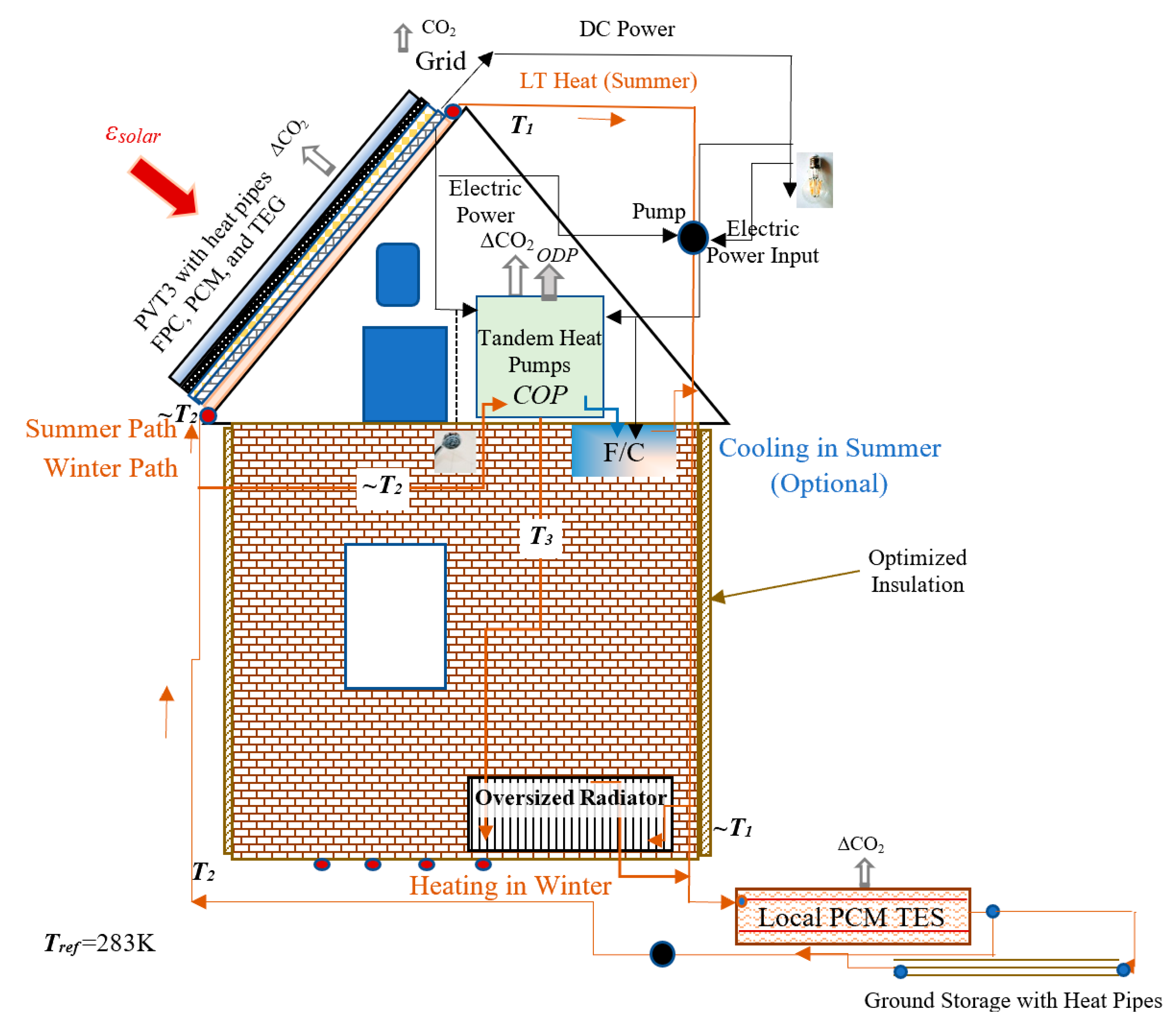
  • The solar district system has been changed to individual solar buildings in a disconnected mode. This approach eliminates to large central thermal storage (ATES) system and eliminates the district pumping stations and pumps. This measure also eliminated the entire district piping, which comes with large embodiments and infrastructural costs. The savings were directed to new heat-pipe radiators and ceiling panels instead of oversizing standard radiators. In the same manner, savings were used to retrofit commercial PVT panels with PVT3 panels.
  • Heat Pump COP optimized additional thermal insulation was applied to exterior walls.
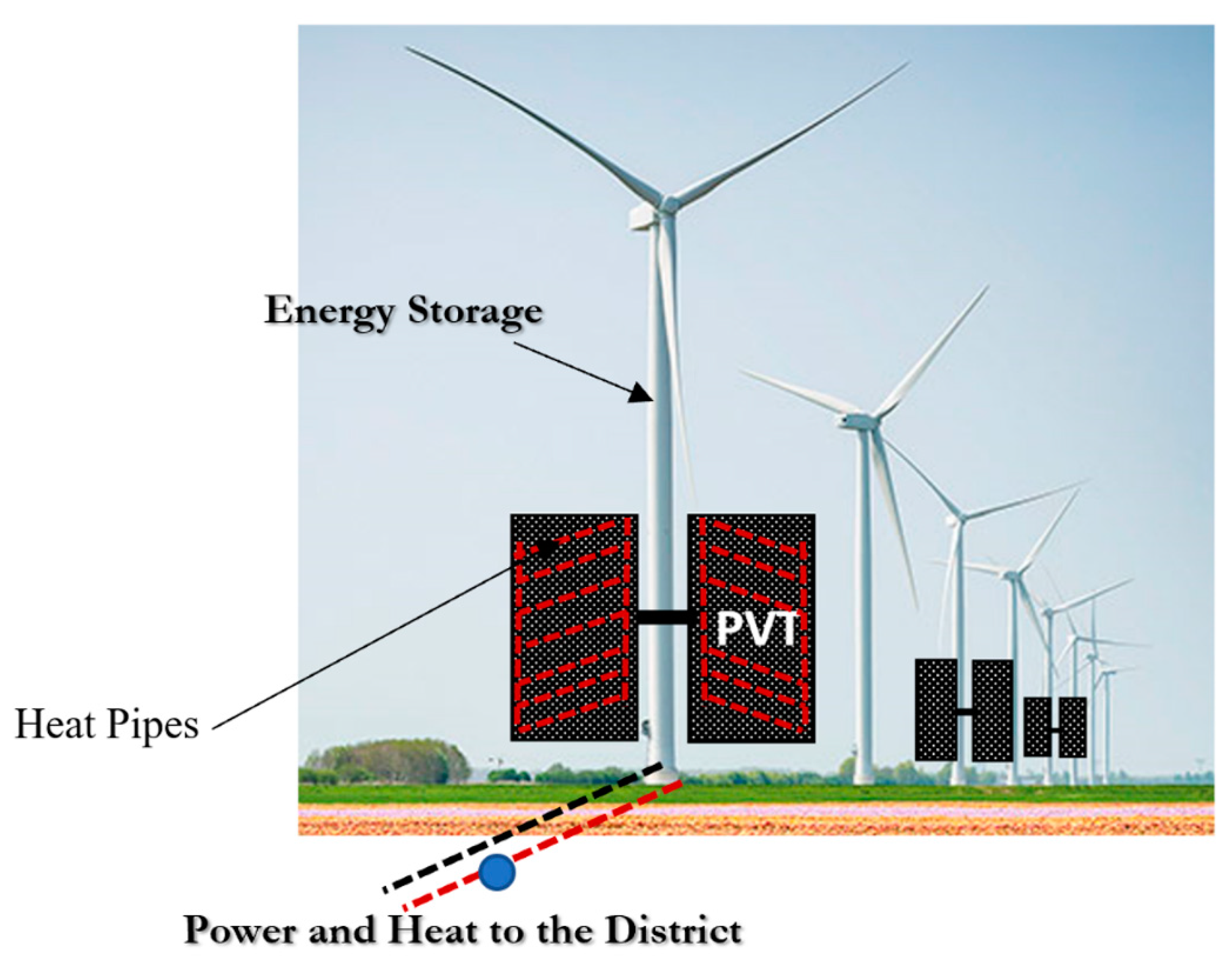
  • Heat pipe technology was extensively used in PVT panels, heating and cooling equipment, and local TES systems.
  • Heat Pump refrigerant was changed from commercial refrigerants to CO2 gas. By using CO2 gas, ozone depletion and global warming effects have been eliminated down to negligible proportions. Furthermore, by using CO2 gas, the same amount is deducted from the emissions stock.
  • Heat pump COP was increased by using two tandem heat pumps. This method reduces the solar electricity demand on board the building and at the same time minimizes CO2 refrigerant leakages from them.
  • Night cooling from the PVT3 panels with a heat pipe connection indoors reduces the cooling loads.

5. Overall Discussion

This paper has shown the importance of retrofitting the building stock for ultra-low heating and ultra-high cooling towards satisfying the Paris Agreement goals. Three prongs of such a transformation to the heat pipe technology in the built environment were identified. These are, namely, hybrid solar-wind power and heat (Cogeneration), radiators and radiant panels with heat pipes for comfort heating and cooling, and thermal energy storage with heat pipes. DeZonnet project was conceptually revised as compared in Figure 32 and Figure 33. The original DeZonnet project is responsible for 4.925 kg CO2/kW-h emissions. Although no fossil fuels are used in the building, direct emissions responsibility is 3.48 kg CO2/kW-h.
On the other hand, the revised building is expected to have minimal emissions responsibility, all of which is only due to nearly-emissions responsibility. Recognition of the missing puzzle between the conventional CO2 emissions “calculations” and the reality is essential to sustainably reduce global warming according to the Paris agreement goals. This difference is about 80% of the calculated values. The current calculations ignore the rationality factor; measures yet to be taken miss about half of the solution opportunities. Figure 35 shows the projection of variables like the 1st Law efficiency, energy rationality, the average unit CO2 emissions factor, the ratio of renewables in the energy stock. For example, in 2020, the global average efficiency in all sectors like mobility, heating, cooling, agriculture, industry, etc., is estimated to be around 0.4. Sectoral penetration of renewables to the energy supply stock is around 20%, the global average of the degree of rationality, which shows how useful work potentials are balanced, among the supply and demand sides in the entire sector is only 0.2 (Reference).
By using these estimates, Figure 36 was prepared. It is understood that unless we recognize the importance of the rationality factor, which is the missing link so far, the targets of the Paris agreement will not be reached. Now, this link is included in Figure 36. According to Figure 36, the carbon-neutral target for 2050, based on simple emission calculations, will be missed by about 0.6 kg CO2/kW-h in the best scenario of today’s strategies. In 2060, the Paris Agreement goal will also be missed by about 0.3 kg CO2/kW-h. Even worse, a 30% renewable target of around 2025 will stay above the requirements for reducing climate crisis and remain there unless all nations abandon the recent natural gas craze and insistence on coal. Generating hydrogen from coal will not be a solution either, and it will stay at a high emissions point if the hydrocarbon economy continues. Figure 35 further shows that whatever measures are taken, we will not reach a negative carbon state unless we embrace nature and incorporate it with rational carbon capture methodologies. As a result, all strategists and energy policymakers need to recognize the importance of the rationality factor in all applications. Then new methodologies, new equipment, machinery, and performance metrics need to be developed to rate these applications towards truly minimum CO2 emissions responsibilities, which have a definite effect on global warming. In this quest, the goal must be to minimize useful work potential destructions. After all, rationality is a matter of wisdom, and we can all do that because all we need is a change of today’s mindset.

6. Conclusions

The Paris Agreement, which most nations have ratified, aims to limit global warming to well below 2, preferably to 1.5 degrees Celsius, compared to pre-industrial levels. This goal corresponds to about 265 ppm (by volume). Figure 1 shows that even the 450-ppm target is almost double the pre-industrial level, even green energy share increases. Figure 36 shows this scale in kg CO2/kW-h energy spending, which was about 0.15 in the pre-industry era. Now, it is 3. Today the global average of exergy rationality is about 20%. Referring to the ideal in Figure 35, the share of renewables will increase, increasing exergy rationality. However, their impact is not entirely linear upon CO2 emissions because there will always be a residual fossil fuel use necessary to offset remaining exergy destructions to manufacture renewable energy systems. The curve at the bottom represents the additional positive impact of heat pipe technology. The figure shows that the Paris Agreement Target of lowering the CO2 emissions below the pre-industrial era level is not precisely possible even with 100% renewables and exergy rationality reaches about 90%. Yet this reduction level is expected to be sufficient such that nature will take over by natural carbon sequestration. Hydrocarbon economy will be useful but must be based on 100% surplus renewables, which is not the case, represented by two points on the figure.
More experiments for heat pipe characteristics and radiator types are required, including field studies. Additionally, more laboratory and field experiments need to be carried out for different configurations, and heat pipe fill chemicals and fill ratio to precisely determine the m and n values. It is also essential that at low temperatures with low-temperature differences in heat pipes, concentric annular heat pipes may be considered, which may further enhance the thermal conductance [49]. The same heat pipe technology may be coupled with the Enover type of radiators to develop new wall panels to take advantage of increasing the radiant heat transfer component at very low heating temperatures from large wall surfaces. Such a system may replace conventional floor heating systems with exergy-demanding circulation pumps and makes it technically feasible to introduce radiant panel technology as a retrofit option also for old buildings without demanding additional pump power by using heat pipes. There is already some research in this subject matter, like Amanowics, L. has investigated how to control the heating capacity with the temperature and supply water of the district energy supply system [50]. He carried out experiments to find the relationship among operational variables and derived design correlations for typical applications. His research, however, did not involve the exergy perspective of the performance.
There are other heat pipe enhancing technologies. For example, Goshayeshi, Goodarzi, and Dahari have investigated the effect of electromagnetic field applied to a heat pipe composed of kerosene/Fe2O3 nanofluid in a copper oscillating heat pipe [51]. In their experiments, the authors have observed that the addition of FE2O3 nanoparticles and the application of an external electromagnetic field improved both the thermal performance and the heat transfer coefficient. Their experiments indicated a 16% improvement in thermal performance when the nanoparticles and magnetic field were applied. The magnetic field typically demanded electrical power with a 2-ampere current for 0.274-tesla magnetic field at their experimental scale needs to be taken into account. In practice, the electrical energy and exergy involved in spending for magnetization must be less than the additional energy and exergy gains by applying the field for thermal performance enhancement. It must be noted that usually, the thermal exergy gain has low unit exergy while electrical power exergy is 0.95 kW/kW.
Menlik et al. [52] have investigated the effect of MgO/Water nanofluid. They observed an improvement of 26% capacity increase compared to plain water in their laboratory test using a straight copper tube at 200 W heating power and 7.5 g per second flow rate. The heat pipe was 1 m long with an inner diameter of 13 mm.
These two research papers show the increasing interest in heat pipes with enhancing nanofluids. These experiments need to be further expanded from the lab scale to the practical field scale, especially for revealing their potential impact for decarbonization with new equipment for low-temperature heating and high-temperature cooling, as exemplified in this paper.
The main target should be decarbonization, as stated above. Heat pipes use less power to distribute the heat more effectively and offer an opportunity to reach the Paris Agreement title as shown by the bottom curve when coupled with 5DE district energy systems in three prongs mentioned in this paper. These prongs are heat pipes in heating and cooling equipment, solar PVT systems, and onsite thermal storage. In the first prong, they reduce the need for material oversizing at low supply temperatures and demand less pumping energy. These features reduce the embodiments and the need for exergy offsets in transition to the renewable energy system, as explained above, regarding Figure 35. The second prong may need further clarification. For example, if a solar PVT system shown in Figure 18 uses heat pipes and replaces the onboard coolant circulation pump with an electrical power demand at design conditions, P, the following carbon emission savings per hour of solar PVT operation may be estimated:
C O 2 s a v i n g = 0.9   P × P E F × 0.3 = 0.675   P   ( kg   CO 2 / h )
Here, P is the electric power demand of the circulation pump (kW), PEF is the primary energy factor, which is currently 2.5 for the EU countries, and 0.3 kg CO2/kW-h is the average emissions factor for the fuel mix in the power sector. If P is 50 W (0.05 kW) for a typical single PVT panel of 1 m2, then removing the pump with heat pipes in the design will save 0.034 kg CO2 per hour during its life cycle. If the total number of hours is 40,000, then this single heat pipe PVT will save a total emission of around 1.4 tons of CO2. The overall impact may also be seen in Table 2 and Table 3 regarding Figure 33 and Figure 34. According to Figure 36, the overall impact of heat piping on the heating and cooling sector by the year 2050 may be estimated to be 50% more reduction in CO2 emissions when coupled with 5DE systems.
With the current climate emergency, which more than 60 countries have already declared, technical feasibility on the exergy basis has become more dominant over economic feasibility [53]. The result is also an economic advantage when coupled with material weight savings, reduced need for heat pumps, and operating costs compared to oversized standard equipment. Therefore, it seems to be a win-win situation that has to be further explored. Shukuya [54] has already pointed out the potential benefits of the exergetic approach ranging from human comfort to power plants, mobility, and particularly the built environment with a wide variety of discussion on the built-environmental space such as heating, cooling, lighting, and others.
  • This paper is expected to holistically extend the vision already opened by Shukuya, to the policymakers for improving their road maps and expanding their current strategies for decarbonization. The following takeaways may be recognized:
  • All EU guides and directives need to be revised to include the exergy concept [5,6]
  • Development and commercialization of low-temperature heating and high-temperature cooling equipment with minimum CO2, energy, cost, exergy embodiments, and affordable enough for easy retrofit must be prioritized, and R&D activities supported specifically with EU grants and other mechanisms, worldwide.
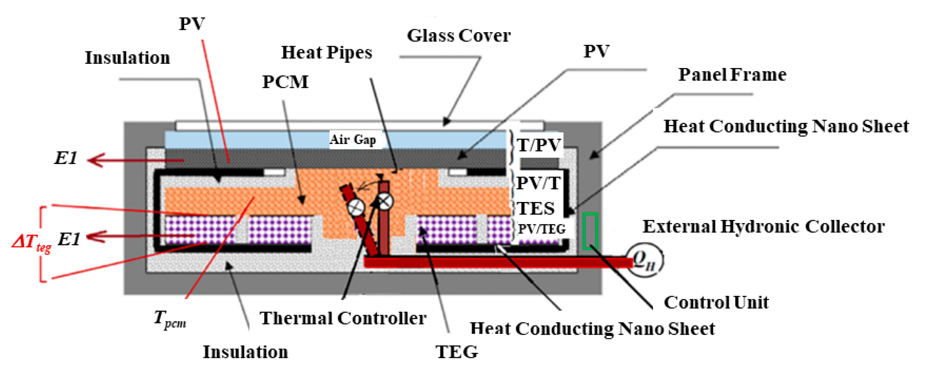
  • Heat pipe technology for aiming the maximum efficiency and minimum exergy losses, savings in material, and weight in the buildings must be prioritized along three main vectors, namely the solar PVT systems, short-term energy storage (With PCM), and the equipment themselves.
  • Until new heating and cooling equipment widely penetrate the building sector, tools for optimum design of oversizing the existing heating and cooling equipment and assisting with high-COP heat pumps in a tandem format must be developed and provided to the design market and building engineers and architects.
  • New-generation solar PVT systems must be implemented to utilize the solar exergy for given solar insolation areas in and around the buildings.
  • Public and government awareness about the exergy dimension of the solution for global warming must be raised by publications, seminars, and online educational packages. It must be emphasized that the methodology presented in this paper makes the information transition and practice much easier to grasp and implement.
  • District energy concepts with low-temperature heating and high-temperature cooling are rising in the political and engineering agenda. This seemingly effective way of decarbonization, the district thermal exergy circulated versus the pumping exergy demand must be noted by policymakers, and future designs for 100% RHC cities must be a prerequisite.
  • Total electrification by heat pumps concept is also on the rise by the influence of the heat pipe industry. Yet according to the 2nd Law of Thermodynamics, as clearly explained in this paper, COP values must be increased by innovations, and optimum cascading of heat pumps must become a general practice.
  • The concept of Renewable Energy Cities must be transitioned to the concept of Renewable Exergy Cities if sustainable decarbonization is the real agenda with the recognition that decarbonization is a matter of minimizing exergy destructions, beyond increasing the energy efficiency.
  • Today, exergy becomes first within the general energy, environment, water, and welfare nexus. This must be widely acknowledged by all means (see [53]).
  • It must be realized that the exergy rationality concept is not only a game-changer but moreover is a game maker that must be taken into an advantage.
  • Sometimes low-temperature district energy systems may not be effective in CO2 emissions responsibility. Then individual green buildings or smaller-sized districts must be on the energy agenda.

Author Contributions

Conceptualization, M.Ç. and B.K.; methodology, B.K.; resources, B.K.; writing—original draft preparation, B.K.; writing—review and editing, B.K.; visualization, B.K.; supervision, M.Ç.; project administration, M.Ç. and M.Ş. All authors have read and agreed to the published version of the manuscript.

Funding

This research received no external funding.

Institutional Review Board Statement

Not applicable.

Informed Consent Statement

Not applicable.

Conflicts of Interest

The authors declare no conflict of interest.

Nomenclature

Symbols
ApSolar Panel Area, m2
AUSTArea Average of Un-Conditioned Indoor Surface Temperatures, K
cEquipment heating capacity factor (Equations (48) and (61)), kW/K
c`Unit CO2 emission value of fossil fuel, kg CO2/kW-h
c``, c```Constants in Equation (35)
CpSpecific Heat, J/kg K
CO2Direct CO2 emissions, kg CO2/kW-h
COPCoefficient of Performance (Heat Pump)
dConstant in Equation (60)
dTtTemperature Deficit Between Optimum Heat Pump Output (supply) Temperature and Optimum Equipment Input Temperature, (Equation (50)) K
C1TfhpTg, K (Figure 24)
C2TfeqTa, K (Figure 24)
CeqLife-Cycle Cost Factor for Equipment, €/kW-h [46]
ChpLife-Cycle Cost Factor for Heat Pump, €/kW-h [46]
CtLife-Cycle Cost Factor for Auxiliary Heater, €/kW-h [46]
Co-tLife-Cycle Cost of Auxiliary Heater (to be added to equipment and heat pump life-cycle costs)
EElectric Power, kW
ELCExergy-Levelized Cost, €/(kWEXpeak/m2)
ELCCO2Exergy-Levelized CO2 Emissions Cost, kg CO2/(kWEXpeak/m2)
EXHThermal Exergy, kW
F`Oversizing Factor (Equation (32))
GWPGlobal Warming Potential
hHeat Transfer Coefficient, kW/m2K
IDInternal Tube (Pipe) Diameter, m
InSolar Insolation Normal to the PV Panel Surface, kW/m2
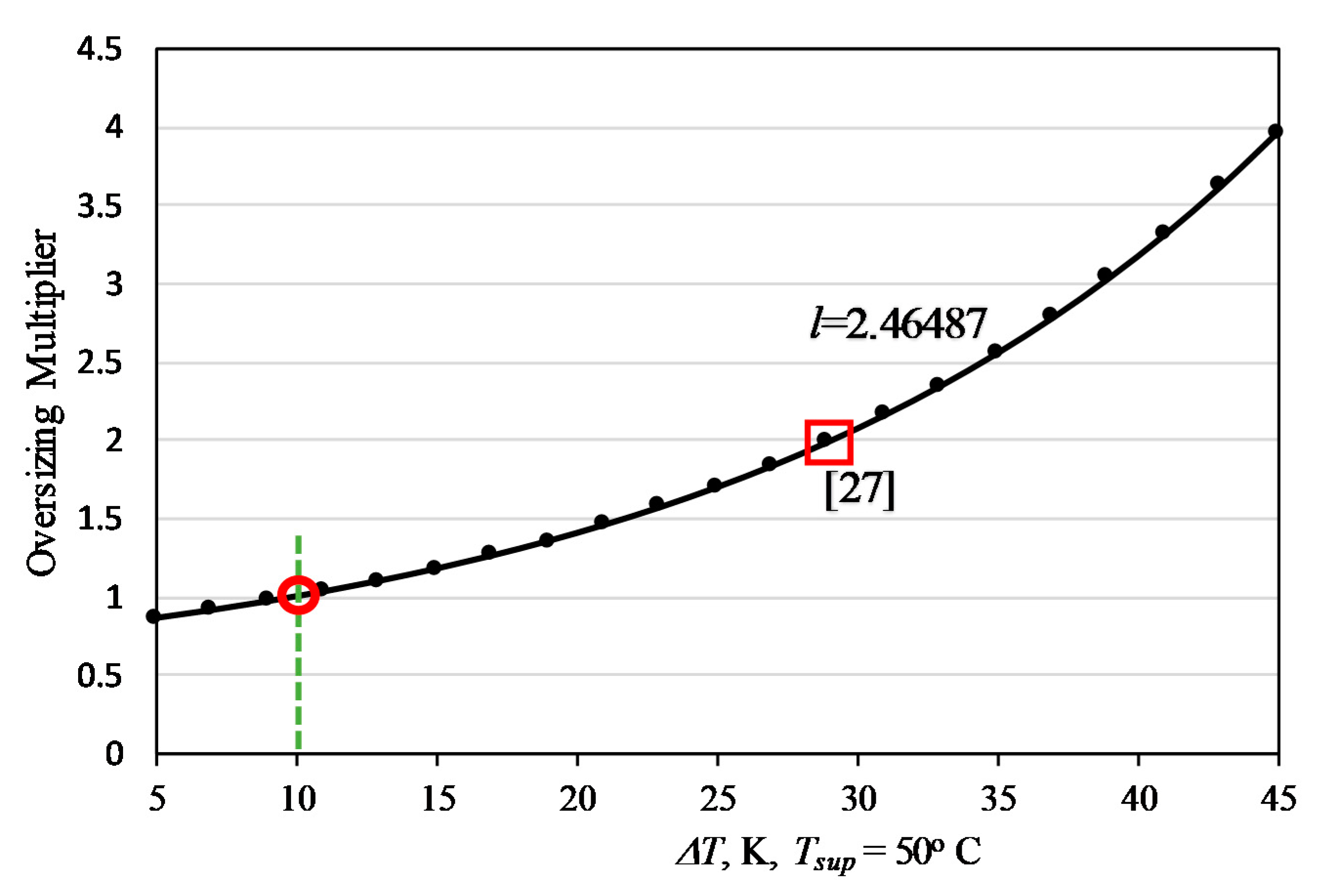
lOversizing Multiplier in Equation (11)
LLength of District Loop, m
LPLife of Solar Panel
MOCTube Spacing on Centers, m (Equation (38))
nNumber of Floors in a Building
ODIOzone Depleting Index
ODPOzone Depletion Potential
REXExergy-based share of renewable energy sources by installed capacity in the energy stock
NpNumber of Parallel Piping in the District Energy System
NfTemperature Life Cycle
PPump Power, kW
q, rHeat Pump COP multipliers (Equation (56)), q is dimensionless r has a unit of K−1
QHeat Load, Heat Supply, kW
QoRated Heat Capacity, kW
QWPQo/Wp, kW/kg
qHeat Flux, kW/m2
rThermal Resistance, m2K/W
RRMRadiator Capacity Increase per Oversizing Ratio, kW/kg
TTemperature, K or °C
tTime, s
U`Heat Load Coefficient of The Building, kW/K
V ˙ Volumetric Flow Rate, m3/s
WWeight, kg
wConstant in Equation (25)
WDWeight Metric (Equation (47)), kg−1
WpWeight of the Radiator, kg
WWWeight of Water Content of the radiator (SR), kg
yConstant in Equation (28)
Greek Symbols
ΔCO2Nearly-Avoidable CO2 Emissions Due to Exergy Destructions, kg CO2/kW-h
ΣCO2Total CO2 emission (Sum of Direct and Nearly-Avoidable Emissions), kg CO2/kW-h
ΔHHeat Deficit, kW
ψRRational Exergy Management Efficiency
EUnit exergy, kW/kW
BThermal constant of PV Efficiency
η, ηIFirst-Law Efficiency
RMass Density, kg/m3
Subscripts
aIndoor Air
BoilerBoiler
DDistrict
demDemand
desDestroyed
eqEquipment
fCarnot Cycle-Based Equivalent (Virtual) Energy Source Temperature-related or adiabatic flame temperature of fossil fuel, or source temperature of renewable thermal energy sources-related, fuel
fuelFuel
HHeat
HEHeat Exchanger
inInner, input
insThermal Insulation
mMean (Average) Temperature, K
maxMaximum
moElectric Motor
0Original (Design, Rated) Value
optOptimum
PPanel, pump
outOut
peakPeak
refReference
SSteam
supSupply
ULUltra-Low (Temperature)
xExergy
Superscripts
`Modified, Secondary
nEquipment Heating Capacity Exponent
mAdditional Equipment Heating Capacity Exponent
Abbreviations
ATESAquifer Thermal Energy Storage
1DE (or 1G)First-Generation District Heating
5DEFifth-Generation District Energy System
5DE+Beyond 5DE
ACAlternating Current
ATESAquifer Thermal Energy Storage
BAUBusiness as Usual
CCCarbon Capture
CCSCarbon Capture and Storage
DCDirect Current
EHPEnover Heat Pipe
EUEuropean Union
F/CFan Coil
GGeneration (District Energy System)
GHGGreen House Gas Emissions
HPRHeat Piper Radiator
HVACHeating, Ventilating, and Air Conditioning
IAQIndoor Air Quality
HPHeat Pump
IEAInternational Energy Agency
LTLow-Temperature
LowExLow-Exergy (Building)
OECDOrganization for Economic Co-operation and Development
PCMPhase-Changing Material
PMPPTDirect Power MPPT (Maximum Power Point Tracking)
PVPhotovoltaic Cell (Panel)
PVTPhoto-Voltaic-Thermal
PVT1First-Generation (Simple) PVT
REMMRational Exergy Management Model
100REC100% Renewable Energy City
100REXC100% Renewable Exergy City
RHCRenewable Heating and Cooling
SRStandard (Conventional) Hydronic Radiator for Indoor Heating
TESThermal Energy Storage
TEGThermo-Electric Generator

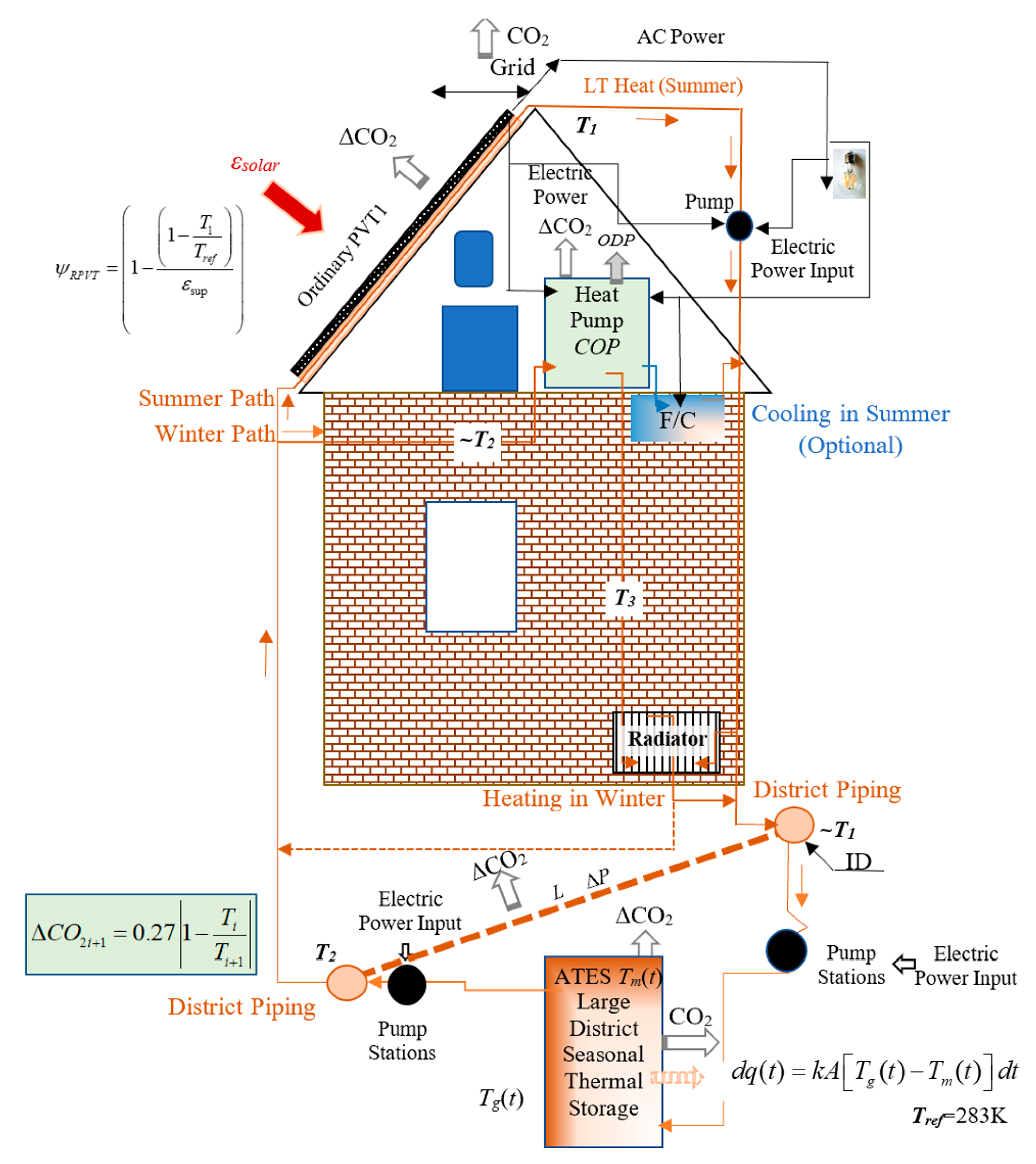
Appendix A. Explanation of Figure 2

Figure 2 is a new 2-D graphical representation of the exergetic relationship among temperatures, namely ΔT, Tref, Ta, and T`sup (Exergy Triangle). The side TaTref represents the unit demand exergy. The side T`supTref represents the unit supply exergy. The side Ta–(T`sup − 1/2 × ΔT) represents the exergy of a unit thermal load (Q = 1 kW), EXH. The triangular area Δs represents the optimization objective, which needs to be maximized within the given temperature constraints and given design temperatures.
O F = Δ s = 1 2 ( T s u p 1 2 Δ T T r e f ) × ( T a T r e f )   ( Maximize )
s.t.
  Q c ( T s u p 1 2 Δ T T a ) n ,   therefore , ( c   and   n   are   the   equipment   performance   factors )
T s u p Q c n + 1 2 Δ T + T a
ΔT, Ta, T`sup are the optimization variables with the non-negativity conditions:
( T s u p T r e f ) > ( T a T r e f ) > 0
ΔT ≥ 5 K
300 K ≥ Ta ≥ 290 K
(Depending upon the heating or cooling system, Relative Humidity, and AUST)
The objective function is to maximize ψR and thereby minimize ΔCO2 responsibility by minimizing Δs.
ψ R = ε d e m ε s u p = ( T a     T r e f T a ) ( T s u p     T r e f T s u p ) = ( T a     T r e f ) ( T s u p     T r e f ) ( T s u p T a )       ( Maximize )
From Equation (A1), (TaTref) = 2Δs/(T`sup − Tref). This relationship simplifies Equation (A7) for a design input of k = T`sup/Ta
ψ R = 2 k Δ s         ( Maximize )
s.t.
ψR < 1 (v) Maximum ψR yields minimum ΔCO2 through Equation (A3):
Δ C O 2 = ε s u p ( 1 ψ R )
In Figure 2, with the application of over insulation to the building, the supply exergy, εsup, and the triangle area decrease, which means that ψR also decreases. According to Equation (A9), any decrease in εsup reduces ΔCO2, but at the same time, any decrease in ψR, according to Equation (A9), increases ΔCO2. A small decrease in Ta may offset this increase if indoor comfort requirements permit. At any rate, this discussion shows that it is also possible to determine an optimum over insulation by using Figure 2.
Any design change in Ta to T`a decreases the area of the bounded triangle when supply temperature, reference temperature, and ΔT are kept fixed. Thus, this figure graphically optimizes the Rational Exergy Management Efficiency, ψR, and minimizes the ΔCO2 emissions responsibility. If it is possible to decrease the design value of ΔT any further, the constraint (A3) is relaxed so that the area may increase. Therefore Figure 2 may be a useful graphical design tool to optimize the thermal performance of a given design.
A sensitivity analysis is also possible. For example, if everything is kept fixed, but Ta is changed:
ψ R = c ( 1 T r e f T a )
Δ ψ R = c ( T r e f T a 2 ) Δ T a
Here, c is a fixed value if Tref and T`sup are fixed.
c = ( 1 T r e f T s u p ` )
Accordingly, if T`sup is decreased for a given Tref temperature, the sensitivity of ψR on any change in Ta decreases because c decreases.

References

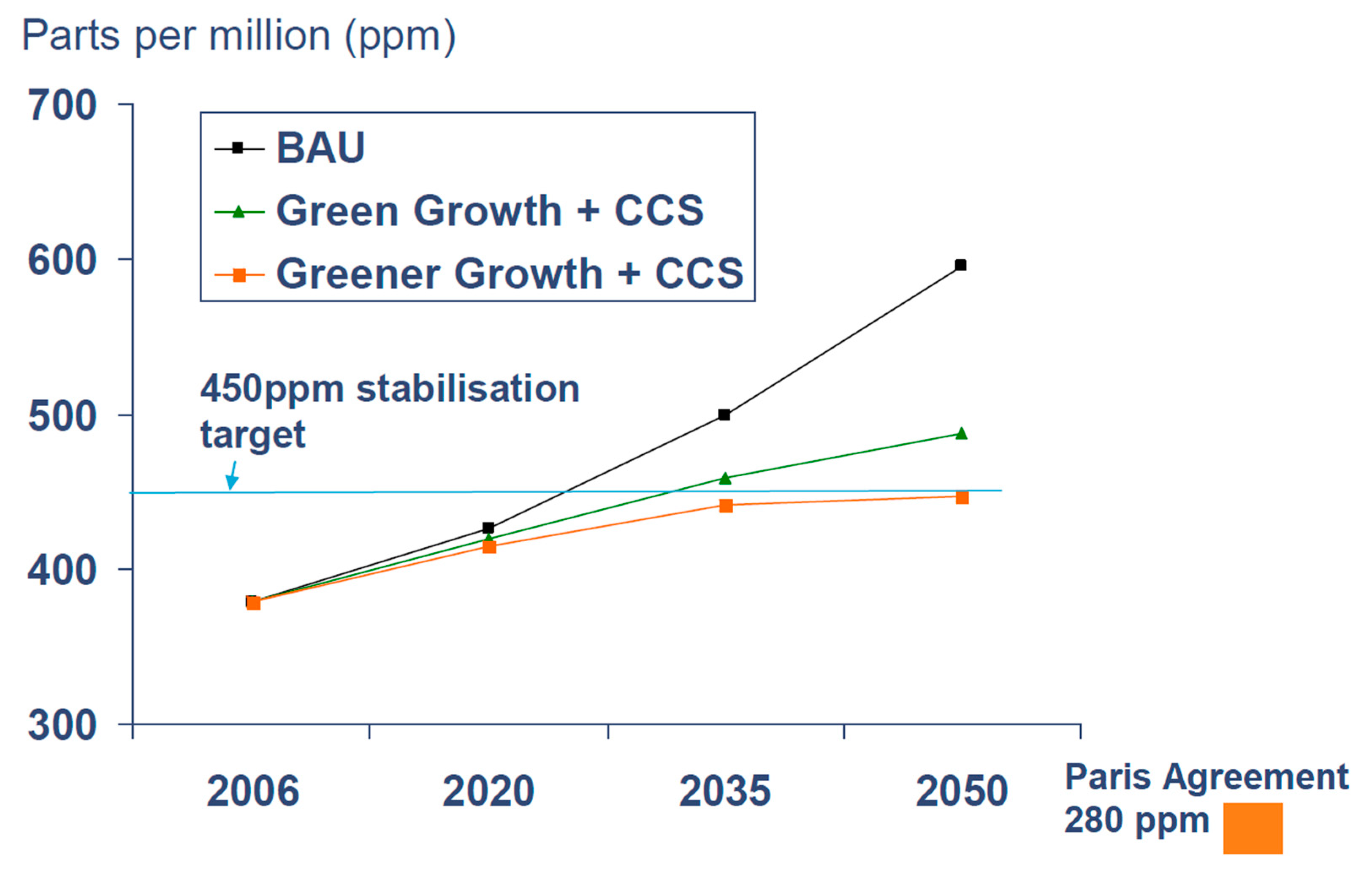
  1. Council Decision (EU). 2016/1841 of 5 October 2016 on the Conclusion, On Behalf of the European Union, of the Paris Agreement Adopted under the United Nations Framework Convention on Climate Change. 2016. Available online: https://eur-lex.europa.eu/legal-content/EN/TXT/PDF/?uri=CELEX:32016D1841&from=EN (accessed on 10 August 2021).
  2. OECD. The OECD Environmental Outlook to 2050 Key Findings on Climate Change. Available online: https://www.oecd.org/env/cc/Outlook%20to%202050_Climate%20Change%20Chapter_HIGLIGHTS-FINA-8pager-UPDATED%20NOV2012.pdf (accessed on 10 August 2021).
  3. Hawksworth, J. The World in 2050 Can Rapid Global Growth Be Reconciled with Moving to a Low Carbon Economy? Price Water Coopers: London, UK, 2008; 22p, Available online: https://www.pwc.com/gx/en/psrc/pdf/world_in_2050_carbon_emissions_psrc.pdf (accessed on 10 August 2021).
  4. ACS. What is the Greenhouse Gas Changes since the Industrial Revolution? ACS Climate Science Toolkit Greenhouse Gases. Available online: https://www.acs.org/content/acs/en/climatescience/greenhousegases/industrialrevolution.html (accessed on 10 August 2021).
  5. Kilkis, B. Sustainability and Decarbonization Efforts of the EU: Potential Benefits of Joining Energy Quality (Exergy) and Energy Quantity (Energy). In EU Directives, A State of the Art Survey and Recommendations, Exclusive EU Position Report; TTMD: Ankara, Turkey, 2017. [Google Scholar]
  6. SE. In a Resource-Constrained World: Think Exergy, Not Energy’ D/2016/13.324/5, Science Europe. Available online: https://www.scienceeurope.org/media/0vxhcyhu/se_exergy_brochure.pdf (accessed on 10 August 2021).
  7. EC. Most Residential Buildings Were Built before Thermal Standards Were Introduced, How Do You Know? Energy, Chart: Breakdown of Residential Building by Construction Year. 2014. Available online: https://ec.europa.eu/energy/content/most-residential-buildings-were-built-thermal-standards-were-introduced_en (accessed on 10 August 2021).
  8. NOVEM. Méér Comfort Metminder Energie, LTV Brochure, Rotterdam, Holland. 2011. Available online: http://www.passiefhuis.info/bouwen/nederland/senternovem/138389_LTV_brochure_tcm24-105131.pdf (accessed on 24 August 2021).
  9. Eijdems, H.H.E.W.; Boerstra, A.C.; Op’t Veld, P.J.M. Low-Temperature Heating Systems Impact on IAQ, Thermal Comfort, And Energy Consumption. In Proceedings of the 21st AIVC Conference, The Hague, The Netherlands, 26–29 September 2000. [Google Scholar]
  10. IEA. EBC Annex 37, LowEx, Literature Review: Side Effects of Low Exergy Emission Systems; Novem BV: Sittard, The Netherlands, 2000; 100p, Available online: https://annex53.iea-ebc.org/Data/publications/EBC_Annex_37_literature_review.pdf (accessed on 10 August 2021).
  11. Kilkis, S. System Analysis of a Pilot Net-Zero Exergy Distric. Energy Convers. Manag. 2014, 87, 1077–1092. [Google Scholar] [CrossRef]
  12. Kilkis, B. Equipment Oversizing Issues with Hydronic Heating Systems. ASHRAE J. 1998, 40, 25–30. [Google Scholar]
  13. Leskinen, N.; Vimpari, J.; Seppo Junnil, S. A Review of the Impact of Green Building Certification on the Cash Flows and Values of Commercial Properties. Sustainability 2020, 12, 2729. [Google Scholar] [CrossRef] [Green Version]
  14. Kılkış, B.; Kılkış, Ş. Rational Exergy Management Model for Effective Utilization of Low-Enthalpy Geothermal Energy Resources. Hittite J. Sci. Eng. 2018, 5, 59–73. [Google Scholar] [CrossRef]
  15. Gawer, R.; Cezarz, N. Stanford University: Economic, Efficient, Green District Low-Temperature Hot Water. In Proceedings of the IDEA Annual Conference, Detroit, MI, USA, 10–13 July 2016. [Google Scholar]
  16. UNEP. District Energy in Cities, Unlocking the Potential of Energy Efficiency and Renewable Energy; UNEP DTIE Energy Branch: Paris, France, 2015; Available online: http://wedocs.unep.org/bitstream/handle/20.500.11822/9317/-District_energy_in_cities_unlocking_thepotential_of_energy_efficiency_and_renewable_ene.pdf?sequence=2&isAllowed=y (accessed on 10 August 2021).
  17. Zhivov, A.M.; Vavrin, J.L.; Woody, A.; Fournier, D.; Richter, S.; Droste, D.; Paiho, S.; Jahn, J.; Kohonen, R. Evaluation of European District Heating Systems for Application to Army Installations in the United States; Report No. ERDC/CERL TR-06-20; Construction Engineering Research Laboratory, US Army Corps of Engineers: Champaign, IL, USA, 2006; 246p. [Google Scholar]
  18. C40 Cities. 98% of Copenhagen City Heating Supplied by Waste Heat, 3 November 2011. 2011. Available online: https://www.c40.org/case_studies/98-of-copenhagen-city-heating-supplied-by-waste-heat (accessed on 24 August 2021).
  19. Schneider Electric. Termis, District Energy Management, User Guide, 5th ed.; Schneider Electric: Ballerup, Denmark, 2012; Available online: https://download.schneider-electric.com/files?p_enDocType=User+guide&p_File_Name=Termis_5_0.pdf&p_Doc_Ref=Termis+Set+Up+Guide (accessed on 14 August 2021).
  20. Bloomquist, R.G.; O’Bien, R. Software to Design and Analyze Geothermal District Heating and Cooling Systems, and Related Air Quality Improvement, World Geothermal Congress. Transactions 1995, 4, 2999–3003. [Google Scholar]
  21. Coudert, J.M. Geothermal Direct Use in France: A General Survey, Geo-Heat Center Quarterly Bulletin; Geoheat Center: Klamath Falls, OR, USA, 1984; Volume 8, pp. 3–5. [Google Scholar]
  22. Jinrong, C. Geothermal Heating System in Tanggu Tianjin, China, Geo-Heat Center Quarterly Bulletin; Geoheat Center: Klamath Falls, OR, USA, 1992; Volume 14, pp. 11–15. [Google Scholar]
  23. Jaudin, F. County Update France. International Symposium on Geothermal Energy Transactions. Geotherm. Resour. Counc. 1990, 14 Pt 1, 63–69. [Google Scholar]
  24. Gudmundsson, O. Distribution of District Heating, 1st ed.; Danfoss: Nordborg, Denmark, 19 September 2016; Available online: https://assets.danfoss.com/documents/57292/BE346042889071en-010101.pdf (accessed on 14 August 2021).
  25. Park, H.; Kim, M.S. Theoretical Limit on COP of a Heat Pump from a Sequential System. Int. J. Air-Cond. Refrig. 2015, 23, 1550029. [Google Scholar] [CrossRef]
  26. Ding, R.; Du, B.; Xu, S.; Yao, J.; Zheng, H. Theoretical Analysis and Experimental Research of Heat Pump Driving Heat Pipes Heating Equipment. Therm. Sci. 2019, 24, 329. [Google Scholar] [CrossRef]
  27. Tol, H.I. District Heating in Areas with Low Energy Houses. DTU Civil Engineering Report R-283 (UK). Ph.D. Thesis, Technical University of Denmark (DTU), Kongens Lyngby, Denmark, February 2015. [Google Scholar]
  28. Kilkis, B. Environmental Economy of Low-Enthalpy Energy Sources in District Energy Systems, HI-02-03-2. In Proceedings of the ASHRAE Transactions, Atlantic City, NJ, USA, 12–16 January 2002; pp. 580–587. [Google Scholar]
  29. Kilkis, B. An Analytical Optimization Tool for Hydronic Heating and Cooling with Low-Enthalpy Energy Resources, Hi-02-14-2. In Proceedings of the ASHRAE Transactions, Atlantic City, NJ, USA, 12–16 January 2002; pp. 968–996. [Google Scholar]
  30. Hongwei, L.; Svend, S. Energy and Exergy Analysis of Low-Temperature District Heating Network. Energy 2012, 45, 237–246. [Google Scholar] [CrossRef]
  31. Wheatcroft, E.; Henry Wynn, H.; Lygnerud, K.; Bonvicini, G.; Leonte, D. The Role of Low-Temperature Waste Heat Recovery in Achieving 2050 Goals: A Policy Positioning Paper. Energies 2020, 13, 2107. [Google Scholar] [CrossRef] [Green Version]
  32. Antal, M.; Cioara, T.; Anghel, L.; Gorzenski, R.; Januszewski, R.; Oleksiak, A.; Piatek, W.; Pop, C.; Salomie, I.; Szeliga, W. Reuse of Data Center Waste Heat in Nearby Neighborhoods: A Neural Networks-Based Prediction Model. Energies 2019, 12, 814. [Google Scholar] [CrossRef] [Green Version]
  33. Grassi, B.; Piana, E.A.; Beretta, G.P.; Pilotelli, M. Dynamic Approach to Evaluate the Effect of Reducing District Heating Temperature on Indoor Thermal Comfort. Energies 2021, 14, 25. [Google Scholar] [CrossRef]
  34. Życzyńska, A.; Suchorab, Z.; Majerek, D. Influence of Thermal Retrofitting on Annual Energy Demand for Heating in Multi-Family Buildings. Energies 2020, 13, 4625. [Google Scholar] [CrossRef]
  35. Yang, W.; Wen, F.; Wang, K.; Huang, Y.; Abdus Salam, M.D. Modeling of a District Heating System and Optimal Heat-Power Flow. Energies 2018, 11, 929. [Google Scholar] [CrossRef] [Green Version]
  36. Suna, H.; Duana, M.; Wua, Y.; Lina, B.; Zixu Yanga, Z.; Zhaoa, H. Experimental Investigation on the Thermal Performance of a Novel Radiant Heating and Cooling Terminal Integrated with a Flat Heat Pipe. Energy Build. 2020, 208, 109646. [Google Scholar] [CrossRef]
  37. Kilkis, B. An Exergy Rational District Energy Model for 100% Renewable Cities with Distance Limitations. Therm. Sci. Year 2020, 24, 3685–3705. [Google Scholar] [CrossRef]
  38. Kilkis, B.; Kilkis, S.; Kilkis, S. Power and Heat Generating Solar Module with PCM, TEG, and PV Cell Layers. Patent TR 2017 10622 B, 21 February 2020. [Google Scholar]
  39. Kilkis, I.B. From Floor Heating to Hybrid HVAC Panel-A Trail of Exergy Efficient Innovations. ASHRAE Trans. 2006, 112 Pt 1, 344–349. [Google Scholar]
  40. ASHRAE. Chapter 6: Radiant Heating and Cooling. In ASHRAE Handbook, HVAC Systems and Equipment; ASHRAE: Atlanta, GA, USA, 2020. [Google Scholar]
  41. Kilkis, B. An Exergy-Based Model for Low-Temperature District Heating Systems for Minimum Carbon Footprint with Optimum Equipment Oversizing and Temperature Peaking Mix. Energy 2021, 236, 121339. [Google Scholar] [CrossRef]
  42. Kerrigan, K.; Jouhara, H.; O’Donnell, G.E.; Robinson, A.J. A Naturally Aspirated Convector for Domestic Heating Application with Low Water Temperature Sources. Energy Build. 2013, 67, 187–194. [Google Scholar] [CrossRef]
  43. Enover. Nano-Heat Aluminum Heat Pipe Radiators, Main Catalog; Enover: Ankara, Turkey, 2020; 44p, Available online: https://enover.com.tr/ (accessed on 29 November 2020).
  44. Kilkis, B. Development of a Composite PVT Panel with PCM Embodiment, TEG Modules, Flat-Plate Solar Collector, and Thermally Pulsing Heat Pipes. Sol. Energy 2020, 200, 89–107. [Google Scholar] [CrossRef]
  45. Shebab, S.N. Natural-Convection Phenomenon from a Finned Heated Vertical Tube: Experimental Analysis. Al-Khwarizmi Eng. J. 2017, 13, 30–40. [Google Scholar] [CrossRef]
  46. Kilkis, I.B. Rationalization and Optimization of Heating Systems Coupled to Ground Source Heat Pumps. ASHRAE Trans. 2000, 106 Pt 2, 817–822. [Google Scholar]
  47. Evren, M.F.; Biyikoglu, A.; Ozsunar, A.; Kilkis, B. Determination of Heat Transfer Coefficient between Heated Floor and Space Using the Principles of ANSI/ASHRAE Standard 138 Test Chamber. ASHRAE Transactions 123 (1). In Proceedings of the ASHRAE Winter Conference, Atlanta, GA, USA, 28 January–1 February 2017; pp. 71–82, 4. [Google Scholar]
  48. Mohammadi, S. DeZONNET Project, Amsterdam Economic Board, Amsterdam Smart City, Posted on 20 April 2019. Available online: https://amsterdamsmartcity.com/updates/project/dezonnet (accessed on 14 August 2021).
  49. Song, E.-H.; Lee y, K.-B.; Seok-Ho Rhi, S.-H.; Kim, K. Thermal and Flow Characteristics in a Concentric Annular Heat Pipe Heat Sink. Energies 2020, 13, 5282. [Google Scholar] [CrossRef]
  50. Amanowics, L. Controlling the Thermal Power of a Wall Heating Panel with Heat Pipes by Changing the Mass Flowrate and Temperature of Supplying Water-Experimental Investigations. Energies 2020, 13, 6547. [Google Scholar] [CrossRef]
  51. Goshayeshi, H.R.; Goodarz, M.; Dahari, M. Effect of Magnetic Field on the Heat Transfer Rate of Kerosene/Fe2O3 Nanofluid in A Copper Oscillating Heat Pipe. Exp. Therm. Fluid Sci. 2015, 68, 663–668. [Google Scholar] [CrossRef]
  52. Menlik, T.; Sözen, A.; Gürü, M.; Öztas, S. Heat transfer enhancement using MgO/water nanofluid in heat pipe. J. Energy Inst. 2015, 88, 247–257. [Google Scholar] [CrossRef]
  53. Kılkış, B. Is Exergy Destruction Minimization the Same Thing as Energy Efficiency Maximization? J. Energy Syst. 2021, 5, 165–184. [Google Scholar] [CrossRef]
  54. Shukuya, M. Exergy: Theory and Applications in the Built Environment, 1st ed.; Springer: London, UK, 2013; ISBN 978-1-4471-4572-1. [Google Scholar]
Figure 1. Atmospheric CO2 Concentration Predictions for Three Scenarios, including the business-as-usual (BAU) scenario. From [3].
Energies 14 05398 g001
Figure 2. Exergy Triangle with three sides representing εdem, εsup, and the unit thermal exergy supply, EXH.
Energies 14 05398 g002
Figure 3. Variation of Over Insulation in Terms of (Q`/Q), ψR, and T`eq with the Supply Temperature.
Energies 14 05398 g003
Figure 4. Historical Evolution of District Energy Systems from Steam to 100% Renewables. Developed from [16].
Energies 14 05398 g004
Figure 5. Length of Steam Pipes of Different Diameters in District Energy Systems Over the Years. From [17]. This figure shows that district loop lengths (in meters) composed of steam pipes have been significantly reduced since the 1950–1954 period. First, this results from the transition from steam to hot water, and second the recognition of the fact that pumping power demand-related emissions versus embodied emissions of large pipe diameters have an optimum point, which generally calls for shorter distances and moderately-sized pipe diameters. That is why larger pipes like DN350 pipes are not used anymore.
Energies 14 05398 g005
Figure 6. Heat Pump/Heat Pipe Composite System. From [6,26]. In this system, the heat-pipe radiator acts as a condenser for the heat pump while heats the indoor space at low temperature through the heat pipes.
Energies 14 05398 g006
Figure 7. Change of Series-Oversizing Rates with ΔT. Reference ΔT is taken 20 K at No-Oversizing Condition (Oversizing: 1). Indoor Air Temperature Ta = 20 °C. This figure shows that equipment oversizing increases while ΔT through the equipment is increased. The corresponding ΔT for no-oversizing is 10 K. The point representing Reference 27 shown on the same curve calls for an oversizing multiplier of 2. Large ΔT values are limited due to aeration problems in hydronic circuits and reduction in heating equipment capacity.
Energies 14 05398 g007
Figure 8. Temperature Profiles of the Fluid Flow in Series Oversizing of the Equipment at Different ΔT and Supply Temperatures, Tsup.
Energies 14 05398 g008
Figure 9. Impossible Case 1. Low-Temperature Source is Peaked at the District Plant by Heat Pump(s). Supply temperature is 65 °C, up to 90 °C. This case enables the retention of the standard equipment without any need to oversize. However, more pipe insulation is required to eliminate additional heat losses. The COP of the central heat pump station is not high due to the temperature peaking requirement from 35 °C to 65 °C and higher.
Energies 14 05398 g009
Figure 10. Impossible Case 2. Removal of Central Heat Pumps (Case 1) with Individual Heat Pumps in the Buildings. Standard Equipment Without Oversizing. In this case, each building is equipped with individual heat pumps. The main district supply line has a lower temperature, thus does not require additional insulation. However, because the return temperature will be higher (55 °C) than the temperature of the solar/waste heat (35 °C), this option defeats the purpose of utilizing low-temperature thermal sources. At the same time, the district return piping needs to be additionally insulated.
Energies 14 05398 g010
Figure 11. Case 3: Utilization of Low-Temperature Sources with Oversized, Standard Equipment. In this case, the district loop is at a low temperature. No temperature peaking is necessary because the standard equipment is oversized, and ΔT must be lowest (5 K). This case increases pumping power demand and embodied costs of equipment oversizing.
Energies 14 05398 g011
Figure 12. Case 4. Ultimate Solution for 5DE District Heating with Heat Pipe Radiators (HPR). Heat pipe radiators are more adjustable to low-temperature supply and require less oversizing. Optimization with small heat pumps will be more feasible if temperature peaking is necessary.
Energies 14 05398 g012
Figure 13. Change of Sensitivity with Low District Temperatures. Moving to low source temperatures increases the sensitivity of the thermal response and leads to control issues, although lower supply temperatures enable the broader use of low-temperature resources.
Energies 14 05398 g013
Figure 14. Experimental Heat-Pipe Natural Convector. Fins are attached to horizontal heat pipes. Reprinted with permission, Elsevier, 2021 [42].
Energies 14 05398 g014
Figure 15. Photo of the Prototype Enover Heat-Pipe Radiator (HPR). This prototype was tested in certified labs.
Energies 14 05398 g015
Figure 16. Simplified PVT Thermal and Electric Power Diagram with a Pump, including the heat exchanger, main pump, and the thermal energy storage. PMPPT: Direct Power MPPT (Maximum Power Point Tracking). P ~ 0 if heat pipes are used.
Energies 14 05398 g016
Figure 17. Life of PV cells depending upon the number of Temperature Cycles. This symbolic figure shows that PV cell life decreases with the number of thermal cycles at higher PV temperatures with little or no cooling.
Energies 14 05398 g017
Figure 18. Pumpless Solar PVT System with Heat Pipes, a Flat Plate Collector Layer on the Top, Additional Power Generation with TEG Units, and thermal energy storage with Embodied PCM Layer. Reprinted with permission, Elsevier, 2021 [44].
Energies 14 05398 g018
Figure 19. Hybrid Power and Heat Generation with Wind Turbines and PVT Panels at the Central Plant.
Energies 14 05398 g019
Figure 20. Standard Radiator Performance: Diminishing Effect of Oversizing on the Heating Capacity with the Supply Temperature Drift from the Design Value, Tm = To to TUL and further. Fluid velocity, V drifts from Vo to Vk. ΔT = Fixed. F` is area oversizing H × L.
Energies 14 05398 g020
Figure 21. A Typical Cross-Sectional Top View of a Standard, Finned Radiator. Tm approaches TUL.
Energies 14 05398 g021
Figure 22. Thermal Resistance Diagram for Standard Radiator with Finned Tubes.
Energies 14 05398 g022
Figure 23. Two Types of Radiators with Oversizing to Accommodate Low-Temperature (LT) Heating. Note that the oversizing requirement is more for a standard radiator. Reprinted with permission, Elsevier, 2021 [41].
Energies 14 05398 g023
Figure 24. The Conflict Between Heat Pump and the Heating Equipment. From [46]. At low supply temperatures, in this case, the ground source temperature, the heat pump COP decreases and requires capacity oversizing to maintain the required thermal output. The HVAC equipment also requires oversizing. An optimum mix of heat pump oversizing and equipment oversizing is available at Tfopt (Point C). See Equations (49) and (51).
Energies 14 05398 g024
Figure 25. Temperature Peaking with a Multitude of NHP number of Smaller Heat Pumps in Tandem. Each heat pump experiences a small ΔT; thus, their COP is high. Reprinted with permission, Elsevier, 2021 [41].
Energies 14 05398 g025
Figure 26. Energy and Exergy Gains with Individual COPi value of Two Heat Pumps in Tandem. According to this figure, the break-even COPBE before exergy gain is about 3.4. However, the exergy gain must be high enough to reach zero exergy destruction level, which is COPimin = 10. Reprinted with permission, Elsevier, 2021 [41].
Energies 14 05398 g026
Figure 27. Change of Equipment Heating Capacity, Qi with Mean Temperature, and (n). The relationship is linear for the n = 1 condition, which corresponds to easier control.
Energies 14 05398 g027
Figure 28. Material Embodiments of HPR and SR with Tsup.
Energies 14 05398 g028
Figure 29. Average CO2 Savings for a 10-unit Apartment (100 radiators) During One Heating Season in Ankara.
Energies 14 05398 g029
Figure 30. Variation of Thermal Response Time of SR and HPR Type of Radiators with Tsup.
Energies 14 05398 g030
Figure 31. Response Time Comparisons of HPR and SR in three consecutive cycles.
Energies 14 05398 g031
Figure 32. Heat-Pipe Ceiling Radiator Panels for Cooling.
Energies 14 05398 g032
Figure 33. Original Dezonnet Project: Large Central District Thermal Storage, Heat Pumps, and PVT1 Panels. The terms c is the constant for pressure drop per unit district length, L. ηPM is the pump-motor efficiency.
Energies 14 05398 g033
Figure 34. Heat Pipes at Three Locations: PVT 3, Radiator, and On-site Thermal Ground Storage.
Energies 14 05398 g034
Figure 35. Linearized Estimates for Best-Case Scenario with Renewables Until 2060. While it is expected that the share of renewables will increase (In this figure assumed to be a linear increase with time), renewable system improvements and low-temperature heating and high-temperature cooling equipment in 5DE systems will help to increase exergy rationality and the 1st Law efficiency, resulting in the reduction of CO2 emissions.
Energies 14 05398 g035
Figure 36. ΣCO2 Emissions per Year, kg CO2/kW-h with Linear Penetration Interpolation of Renewables, 5DE District Energy Systems, and Heat Pipe Technology. Developed from [41].
Energies 14 05398 g036
Table 1. Overall Thermal Conductivity of the 3-Phase, Wickless Enover Heat Pipe (EHP).
EHP Position
VerticalHorizontal
Thermal Conductance W/(m × K)Mean Temperature, Tm, °CThermal Conductance W/(m × K)
13,8409013,340
11,9506011,650
9249359050
Table 2. Different CO2 Emissions Responsibilities of the Primary Components of the Original Dezonnet Project (Embodiments are excluded).
ComponentODPGWPODIΔCO2CO2ΣCO2
kg CO2/kW-h
PVT1 pumps---0.150.300.450
Heat Pump05500.1240.0450.33 * + 0.05 **0.425
District Pumps-- 0.70 ***2.5 ***3.20
ATES---0.35 ***0.15 ***0.450
Domestic Pumps---0.200.150.350
Total1.4453.484.925
* CO2 equivalent of ODI (Ozone Depletion Index). ** Annual grid power share of 1/3, assuming natural gas power plant, PEF: 2.5, annual average COP is 3. *** Prorated to each building. Note: Due to the limited amount of data available, some values are estimates.
Table 3. Different CO2 Emissions Responsibilities of the Primary Components of the Revised DeZonnet Project shown in Figure 33 (Embodiments are excluded).
ComponentODPGWPODIΔCO2CO2ΣCO2
kg CO2/kW-h
PVT3 (No pump)---0.05-0.05
Cascaded Heat Pumps01 *Negligible **0.045Negligible0.425
Local TES with PCM and TES---0.01-0.01
Domestic Pumps---0.05-0.05
Total0.155Negligible0.155
* CO2 gas is used as refrigerant. ** Because GWP is only one for CO2.
Publisher’s Note: MDPI stays neutral with regard to jurisdictional claims in published maps and institutional affiliations.

