Numerical Simulation of Two-Stage Variable Geometry Turbine

Abstract

The modern internal combustion engine (ICE) has to meet several requirements. It has to be reliable with the reduced emission of pollutant gasses and low maintenance requirements. What is more, it has to be efficient both at low-load and high-load operating conditions. For this purpose, a variable turbine geometry (VTG) turbocharger is used to provide proper engine acceleration of exhaust gases at low-load operating conditions. Such a solution is also efficient at high-load engine operating conditions. In this paper, the result of an unsteady, three-dimensional (3D) simulation of the variable two-stage turbine system is discussed. Three different VTG positions were considered for those simulations, along with three different turbine speeds. The turbine inlet was modeled as six equally placed exhaust pipes for each cylinder to eliminate the interference of pressure waves. The flow field at the outlet of the 1st stage nozzle vane and 2nd stage rotor was investigated. The simulations showed that the variable technologies significantly improve the efficiency of the two-stage turbine system. The highest overall efficiency of the two-stage system was achieved at 60,000 rpm and 11° VTG position.

1. Introduction

Nowadays, turbochargers are widely used in ICE engines. Such a highly efficient compressor and turbine wheel allow them to increase the power of the engine quickly. Most modern engines are delivered with fixed geometry turbochargers which accelerate exhaust gases at high-load conditions. However, the ICE engine operates at different load conditions. At the high-load engine conditions, the velocity of the exhaust gases is relatively high. It generates a higher torque on the turbine wheel, which relates to a higher power generation. Thus, the engine accelerates faster, which gives the driver better control over the vehicle. However, at the low-load engine conditions, the velocity of the exhaust gases is inadequate to allow for proper engine response. That is why some of the ICE engines use the VTG turbocharger to improve their performance at low-load conditions. The adjustable vane ring is installed before the inlet to the turbine wheel. The actuator controls the position of the variable vanes. At low-load conditions, vanes are positioned at a maximal closed position, significantly reducing their cross-section flow area. This allows to properly accelerate the exhaust gases, which generate proper torque on the turbine wheel. Thus, the engine response is quicker at low-load conditions.

On the other hand, at high-load conditions, the exhaust gas velocity is very high. Thus, the variable vanes are positioned at maximally opened positions. In order to properly match the VTG turbocharger to the engine, detailed calculations are needed.

The preliminary analytical approach for the design of a VTG turbocharger is a necessity. A mean-line design approach is used to predict main geometry turbine features [1,2,3]. This is a quick and reliable method that predicts turbine performance at the mean-line height of the turbine blades. To predict the off-design turbine behavior of a VTG turbocharger, a ratio of the rotor passage’s mean velocity to the rotor’s circumferential velocity is used [4]. Such a method depends mainly on the configuration of the velocity triangle. Another analytical approach is based on the adaptation of loading to flow diagram [5]. The nozzle opening effect is used to deliver the dimensionless flow parameters.

Some researchers performed experimental tests to predict the behavior of the VTG turbocharger. Even though such an approach gives real-time results, it is very cost-demanding. The test rig has to be prepared with the measuring equipment, allowing to capture instantaneous flow parameters. The variable operating flow conditions are mostly delivered by the installed ICE [6]. Some authors investigate the influence of the VTG turbocharger on engine combustion parameters with the opening and closure of the exhaust recirculation valve (EGR) [7,8]. Different variable geometry technologies are also investigated [9]. Such technologies include pivoting vanes and the sliding nozzle ring. Different types of turbine are also included in the experimental research. Some of them include the mixed-flow turbine of a turbocharger under unsteady flow conditions [10]. Moreover, the electrically assisted variable turbochargers are taken into account for experimental tests [11].

The experimental test is very cost demanding. Thus, some researchers focused on a more straightforward method that used one-dimensional (1D) simulations. Such an approach does not require any cost and can provide reliable results. A steady-stage 1D simulations include a discretization of the main components of turbocharger flow passage [12,13,14,15]. The lack of experimental data can be overcome by assuming the fictitious compressor map [16]. Some researchers include a 1D engine model with an active control turbocharging for a VTG turbocharger [17]. Nowadays, technologies allow performing 1D simulations of a VTG turbocharger with machine learning algorithms such as deep reinforcement learning [18,19]. A quasi-steady rotor behavior is a promising approach to perform unsteady simulations [20,21]. In such an approach, turbine parameters are investigated over a closed-loop pulse cycle. However, a 1D simulation is limited to the discretization of the flow passage. A flow structure cannot be investigated using 1D simulations. Thus, more detailed simulation methods are needed.

Three-dimensional simulations allow to investigate flow structure through the turbine blade passage deeply. It allows to analyze the pressure at the blade surface and flow separation at the trailing edge (TE) of the turbine blades. Such a method allows for the investigation of the steady-state control of VTG turbochargers by comparing the pivoting vane and sliding nozzle ring technologies [22]. In both cases, the variable geometry technologies improved the turbine efficiency significantly with low flow structure loss. Some authors performed steady-state optimization of the turbo-generator for different positions of the nozzle vanes [23]. It was found that the highest efficiency was achieved at the medium vane position. A steady-state 3D simulation allows investigating a stator flow field in a twin-scroll turbocharger [24]. Different types of turbine wheels were also taken into account. A unique variable axial-inflow turbocharger turbine was simulated under steady-state conditions [25]. Thanks to the variable geometry, the isentropic turbine efficiency increased to 86.2%. A steady-state, 3D calculations allowed the emission reduction in a combustion chamber of the micro-turbine engine with variable turbine [26]. To reduce the shockwave at the nozzle vanes for the variable turbine with a high expansion ratio, detailed steady-state 3D simulations were performed [27]. Such simulations used a conformal mapping to investigate the radial nozzle in the x-y coordinate system instead of the radial coordinate system. Finally, the unsteady simulations of a VTG turbocharger turbine were performed for six different stagger angles [28]. A minimal number of unsteady, 3D simulations indicate a great need to investigate the turbine flow-field under variable nozzle vane positions.

This article deals with the unsteady, 3D simulation of a two-stage turbine system with VTG vanes positioned before the 2nd stage rotor. This work is a continuation of the authors’ previous paper which is mentioned in Section 3. The reason for this study was to investigate the behavior of the two-stage turbine system under different VTG vane positions. The mentioned literature is greatly limited to the steady-state operation of the turbocharger turbine. Moreover, most of the mentioned articles dealt with the single-stage turbine system with a few cases related to the 3D problems. This paper presents the results of the 3D unsteady simulation and deals with the complex two-stage turbine system. The unique design on the inlet to the 1st stage rotor eliminates the interference of the pressure waves from adjacent exhaust pipes. This is a common problem in multi-cylinder engines. Such a system will be used in a six-cylinder opposed-piston (OP) engine developed at Warsaw University of Technology.

2. Design of Turbine Wheel

The preliminary design of the turbine wheel was based on such parameters as inlet total temperature $T_0^{*}$, inlet total pressure $p_0^{*}$, nozzle vane outlet isentropic temperature $T_{1iz}$, relative angle at the rotor outlet ${\beta }_2$, turbine wheel inlet and outlet mean diameter $D_1, D_2$, and turbine rotational speed $n$.

For the nozzle vanes the calculation were based on estimated temperature drop which allowed to calculate the enthalpy drop $\Delta h_{Diz}$ across the nozzle vane

$$\Delta h_{Diz}=h_0^{*}-h_{1iz}=\frac{c_{1iz}^2}{2}=c_p^{\prime }\left(T_0^{*}-T_1\right)=c_p^{\prime }{T}_0^{*}\left[1-\frac{T_{1iz}}{T_0^{*}}\right],$$

(1)

where $h_0^{*}$ is the inlet total enthalpy, $h_{1iz}$ is the isentropic enthalpy at the nozzle outlet, $c_{1iz}$ is the isentropic velocity at the nozzle outlet, $c_p^{\prime }$ is the mean specific heat y of the exhaust gases, $T_0^{*}$ is the inlet total temperature, and $T_{1iz}$ is the outlet isentropic temperature.

The outlet isentropic velocity $c_{1iz}$, outlet velocity $c_1$, and outlet pressure $p_1$ can be calculated as:

$$c_{1iz}=\sqrt{2\Delta h_{Diz}}=\sqrt{2\frac{k^{\prime }}{k^{\prime }-1}{R}^{\prime }{T}_0^{*}[1-(\frac{p_1}{p_0^{*}}{)}^{\frac{k^{\prime }-1}{k^{\prime }}}]},$$

(2)

$$c_1=\mathsf{\phi }\ast c_{1iz},$$

(3)

$$p_1=p_0^{*}\left[1-\frac{c_1^2}{2{\mathsf{\phi }}^2\frac{k^{\prime }}{k^{\prime }-1}{R}^{\prime }{T}_0^{*}}\right],$$

(4)

where $\mathsf{\phi }$ is the velocity loss coefficient, $R^{\prime }$ is the exhaust gas constant, and $k^{\prime }$is the exhaust specific heat ratio. The value of $\mathsf{\phi }$ changes from 0.94 to 0.97.

The nozzle outlet temperature $T_1$ is calculated as:

$$T_1=T_0^{*}-\frac{c_1^2}{2\frac{k^{\prime }}{k^{\prime }-1}{R}^{\prime }},$$

(5)

The absolute angle ${\alpha }_1$ can be calculated as:

$${\alpha }_1={\alpha }_k-\delta ,$$

(6)

$${\alpha }_k=arcsin\left(\frac{s}{t}\right),$$

(7)

$$\delta =\delta \left(M_1,\frac{s}{t}\right),$$

(8)

$$M_1=\frac{c_1}{a_1},$$

(9)

$$a_1=\sqrt{k^{\prime }{R}^{\prime }{T}_1},$$

(10)

where ${\alpha }_k$ is the angle of the vane trailing edge (TE),$\delta$ is the deviation angle, $s$ is the perpendicular distance between the adjacent vanes,$t$ is the distance between the trailing edges of the adjacent vanes, $M_1$ is the absolute Mach number at the vane outlet, and $a_1$ is the speed of sound at the vane outlet.

The height of the nozzle vane $l_1$ can be calculated using the equation:

$$l_1=\frac{\dot{m}{R}^{\prime }{T}_1}{\pi D_1{p}_1{c}_{1}sin{\alpha }_1},$$

(11)

where $\dot{m}$ is the mass flow rate of the exhaust gases at the inlet to the nozzle vane. The height of the nozzle vane is also the height of the turbine blade at the inlet.

The relative velocity at the nozzle outlet $w_1$ can be obtained from the velocity triangle configuration:

$$w_1=\sqrt{\left[\left(1-\rho \right){\phi }^2+2u_1\phi cos{\alpha }_1\sqrt{1-\rho }+u_1^2\right]}{c}_{1iz},$$

(12)

$$\rho =\frac{\Delta h_{Wiz}}{\Delta h_{Tiz}}$$

(13)

where $\rho$ is the turbine degree of reaction, which represents the amount of the energy recovered in the rotor $\Delta h_{Wiz}$ to the amount of the energy recovered in whole turbine $\Delta h_{Tiz}$.

The relative angle at the nozzle outlet ${\beta }_1$ can be calculated from the velocity triangle:

$${\beta }_1=arctg(\frac{1}{ctg{\alpha }_1-\frac{u_1}{\sqrt{1-\rho }\phi sin{\alpha }_1}}),$$

(14)

The relative velocity $w_2$ at the rotor outlet can be calculated as:

$$w_2=\psi \sqrt{\rho c_{1iz}^2+w_1^2-u_1^2[1-(\frac{D_2}{D_1}{)}^2]},$$

(15)

where $\psi$ is rotor velocity loss coefficient. Its value changes from 0.93 to 0.97.

The absolute velocity $c_2$ at the rotor outlet can be obtained from equation:

$$c_2=\sqrt{w_2^2-2w_2{u}_1\left(\frac{D_2}{D_1}\right)cos{\beta }_2+u_1^2{(\frac{D_2}{D_1})}^2},$$

(16)

The absolute angle ${\alpha }_2$ of the velocity $c_2$ can be obtained from the velocity triangle:

$${\alpha }_2=arctg\frac{1}{ctg{\beta }_2-\frac{u_2}{w_{2}sin{\beta }_2}},$$

(17)

The expansion work of the rotor $l_{uT}$, as well as the rotor expansion efficiency ${\eta }_{uT}$ can be calculated using equations:

$$l_{uT}=\frac{c_1{}^2-c_2{}^2}{2}+\frac{w_2{}^2-w_1{}^2}{2}+\frac{u_1{}^2-u_2{}^2}{2},$$

(18)

$${\eta }_{uT}=\frac{\left(c_1{}^2-c_2{}^2\right)+(w_2{}^2-w_1{}^2)+(u_1{}^2-u_2{}^2)}{c_{1iz}^2},$$

(19)

The total turbine efficiency can be calculated with equation:

$${\eta }_T=\frac{l_t}{\mathsf{\Delta }{h}_T}{\eta }_m={\eta }_{uT}\left(1-{\xi }_{\delta }\right){\eta }_m,$$

(20)

where $l_t$ is the expansion work of the turbine stage, $\mathsf{\Delta }{h}_T$ is the enthalpy drop trough turbine stage, ${\eta }_m$ is the mechanical efficiency, and ${\xi }_{\delta }$ is the coefficient indicating losses generated by the leakage between the tip of the turbine blade and turbine housing.

Lastly, the turbine blade height at the outlet is calculated as:

$$l_2=\frac{\dot{m}{R}^{\prime }{T}_2}{\pi D_2{p}_2{w}_{2}sin{\beta }_2},$$

(21)

3. Model Preparation

This paper continues the research from the authors previous research paper [29]. Previous research paper dealt with the two-stage turbine system with the single, fixed position of the stator vanes. In contrast to the mentioned paper, the critical point of this work is the influence of the different positions of the variable vanes on the two-stage turbine system. The numerical model was generated based on the K44 turbine wheel as shown in Figure 1.

The turbine wheel was scanned using the AKON smartSCAN 3D HE scanner. The turbine was placed on the turntable and a total number of 60 scans were made during the 360° revolution of the turntable. After the scanning process, the scanned model was corrected using computer-aided design software. The geometrical features of the K44 turbine wheel are shown in

Table 1. The parameters of turbine wheel.

B&W K44 Turbine Wheel
Type	Radial inflow
Number of blades	12
Inlet diameter (mm)	120
Outlet diameter (mm)	140
Inlet blade height (mm)	125
Outlet blade height (mm)	30

[29].

The model consisted of six, equally placed exhaust pipes connected to the 1st stage turbine wheel as shown in Figure 2a.

The cross-sectional, hydraulic diameter of the exhaust pipes was 80 mm. The total length of each exhaust pipe was 1500 mm.

The cross-sectional view of the numerical model is shown in Figure 2b. The 2nd stage nozzle vanes were variable to control the backpressure in the upstream direction. The geometry of the 1st and 2nd stage turbine wheels was the same. The diffuser and inter-stage pipes were iteratively modeled to adjust the length and the cross-sectional area to reduce the pressure loss. The 1st stage nozzle vanes were set at the angle of 30°.

Figure 2c shows the detailed view of the tip clearance gap domain and the 1st stage nozzle vane. Each exhaust pipe had its nozzle vane to accelerate the exhaust gases before entering the 1st stage turbine wheel. The tip clearance gap domain was modeled to investigate the leakage between the adjacent exhaust pipes. The height of this gap was set to 3 mm.

4. Numerical Domain

The numerical model was made of the total number of 24 domains: (×6) exhaust pipes, (×6) tip-clearance gaps, (×6) first-stage nozzle vane domains, 1st stage turbine wheel, diffusor, inter-stage pipes, VTG vanes, 2nd stage-turbine wheel, and outlet. The hexahedral mesh was generated on exhaust pipes, tip-clearance gaps, first-stage nozzle vanes, diffusor, inter-stage pipes, VTG vanes, and outlet as shown in Figure 3a–d.

However, a polyhedral mesh was generated on both the 1st and 2nd stage rotors due to its complex geometry as shown in Figure 3e. The polyhedral mesh was chosen to reduce the number of the elements on both rotors without increasing the numerical error. The mesh was generated using the ICEM CFD software.

5. Simulation

The transient simulations were performed using the ANSYS FLUENT software. The inlet mass-flow-rate boundary condition was applied at the inlet of exhaust pipe. On the other hand, the pressure outlet boundary condition was applied at the outlet as shown in Figure 4a.

The inlet mass flow rate was changing from 0 to 1.0 kg/s during the opening of the exhaust valve in each exhaust pipe. Figure 4b shows changes in the mass flow rate of each exhaust pipe during the single revolution of the crankshaft.

The simulations were carried out for a 6-cylinder, two-stroke engine, and that is why the interval between mass flow rate profiles for each exhaust pipe was a 60° crank angle degree (CAD). The mass flow rate profiles were obtained from 1-D simulations. The parameters of the engine are shown in

Table 2. The operating parameters of the 6-cylinder, 2-stroke engine.

Engine Parameters
Number of cylinders	$6$
Type	2-stroke
Rotational speed $\left(\mathrm{rpm}\right)$	1500
Cylinder bore (mm)	115
Cylinder Stroke (mm)	195.2
Displacement (cm3)	24,000
Crankshaft angle step (deg)	0.1

[29]. The parameters of the boundary conditions are shown in

Table 3. The parameters of the boundary conditions.

Inlet Boundary Conditions
Type	Mass-flow-inlet
Mass flow rate (kg/s)	$0÷1$
Total temperature (K)	1100
Total pressure (Pa)	240,000.0
Outlet Boundary Conditions
Type	Pressure-outlet
Outlet pressure (Pa)	100,000
Outlet temperature (K)	500

[29].

The 1st and 2nd stage rotor domains were rotating at the same rotation speed. To capture the instantaneous changes of the key parameters during the single time step, the sliding mesh method was chosen. In such a method, the whole domain rotates with specified rotational speed while the stationary vanes domain is linked with the rotational domain via the sliding interface. Such a solution allows transferring averaged parameters between both domains during each time step. In this model, the 1st stage rotor was linked to (6) 1st stage nozzle guide vane domains and (6) tip clearance gap domains via the sliding interface. Moreover, the 2nd stage rotor was linked to the VTG vanes domain and outlet domain via the sliding interface. The other stationary domains were linked with each other by stationary interfaces.

The simulations were performed for three different turbine speeds: 40,000 rpm, 50,000 rpm, and 60,000 rpm.

The key point of the research was the investigation of the model parameters during three different openings of the VTG vanes, as shown in Figure 5.

Figure 5 shows three different configurations of the VTG openings of the 2nd stage turbine wheel. For the research purposes, the 2nd stage turbine vanes were set at the three angles, i.e., 30°, 20°, and 11°, which represents the maximal opened, medium, and maximal closed position of the variable vanes. Figure 6 shows the mesh of the VTG vanes for three different openings.

The numerical time step was set to 1.1 × 10⁻⁵ s to precisely capture the instantaneously changing flow parameters at the interface of rotary and non-rotary domain. The pressure-velocity coupled scheme was used to provide stable calculations. Due to the unstructured mesh, the second-order discretization scheme was used for the pressure, density, and momentum. For the time formulation, the first-order implicit scheme was used with the Courant Number of 10.0. The single-equation Spalart–Allmaras (SA) turbulence model was used [30]. This turbulence model assumes that the modified turbulent kinematic viscosity $\tilde{\vartheta }$ is linear in the near-wall region, reducing computational time. Moreover, the SA turbulence model is more tolerant for highly unstructured mesh. With such a small time step, the average computational time was 12 days for a single revolution of the crankshaft. The parameters of the computer are shown in

Table 4. The parameters of the computer.

Computer Parameters
Number of cores	4
Processor type	Inlet Core i7
Random-access memory (Gb)	32
Graphics processor unit memory (Gb)	0.512

.

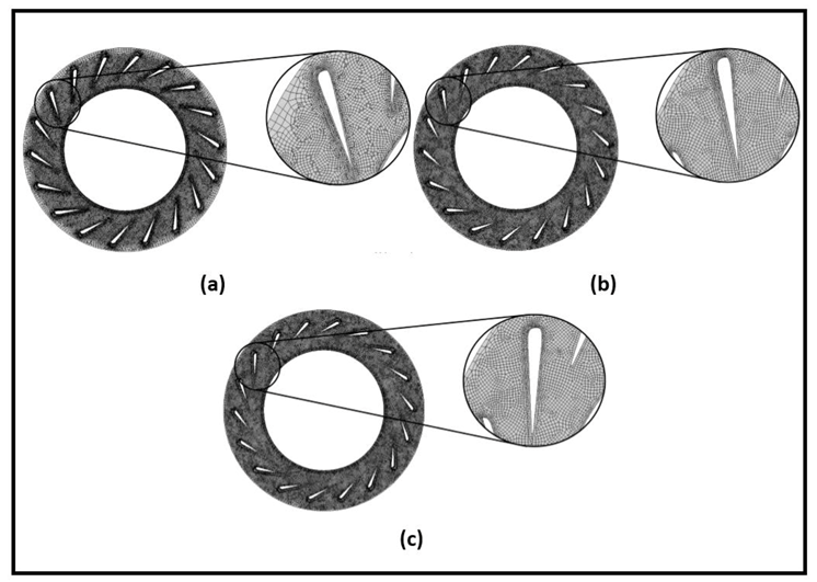
5.1. Mesh Independence Study

The mesh independence study was performed prior main calculations. The mass-weight average total pressure changes were investigated at different mesh densities during the single revolution of the crankshaft. The independence study was performed on exhaust pipes, 1st stage rotor, VTG vanes, and 2nd stage rotor. Figure 7 shows the independence mesh study.

Figure 7 shows that, with the increase of the number of elements in each domain, the pressure changes were decreasing.

Table 5. The number of cells for each domain.

Domain	Number of Elements
Exhaust pipe (×6)	43,200
First-stage nozzle vane (×6)	18,036
Tip clearance gap (×6)	540
1st stage rotor	1,340,000
Inter-stage pipes	168,018
VTG vanes	711,000
2nd stage rotor	1,340,000
Outlet	374,850

shows the number of elements in domain [29].

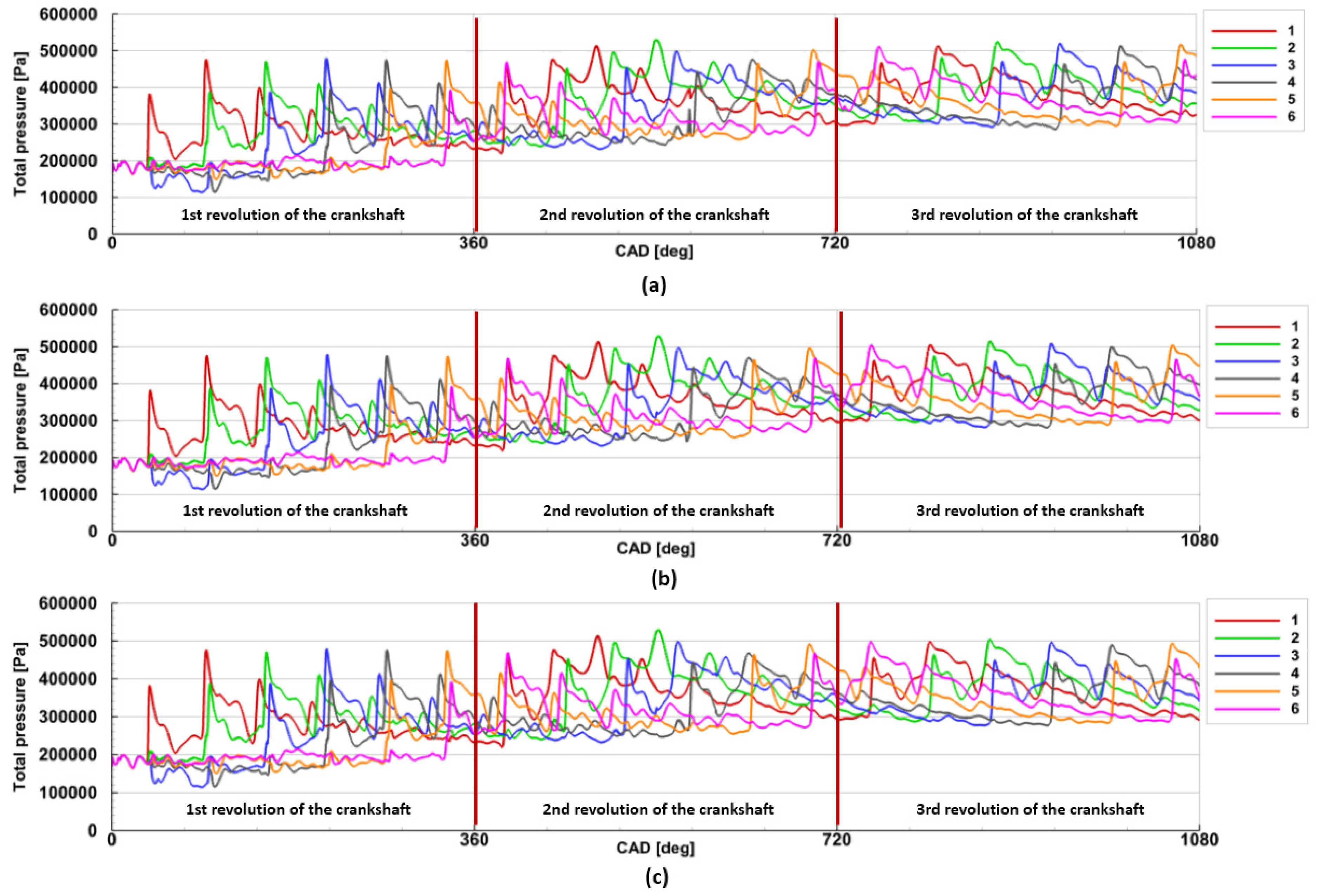
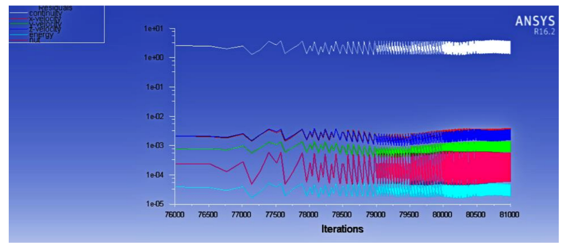
5.2. Simulation for Three Revolutions of the Crankshaft

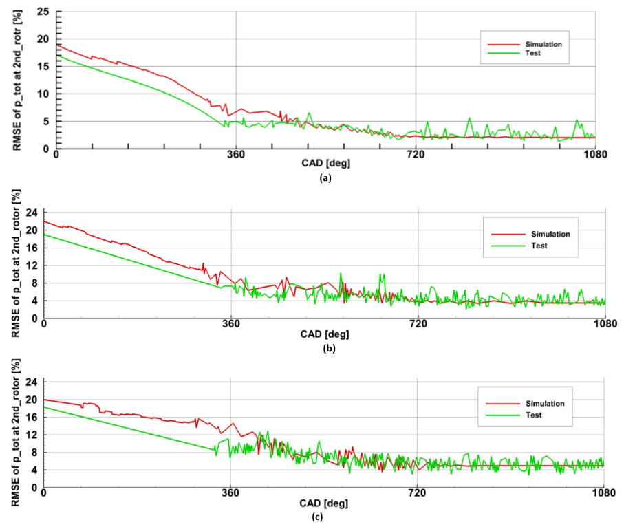
The simulation was performed until the end of the third revolution of the crankshaft to obtain identical pressure changes in each exhaust pipe for every turbine speed.

Figure 8, Figure 9 and Figure 10 show the pressure variations at the inlet to the 1st stage rotor for the three different turbine speeds and three different VTG openings during the three revolutions of the crankshaft.

Figure 8 presents the pressure plot during the maximal opening of the VTG vanes. One can see that the pressure changes during the 3rd revolution of the crankshaft were almost the same for each exhaust pipe. In this case, pressure changed from 300,000 Pa to 510,000 Pa. The lowest, maximal pressure values were achieved at the turbine speed of 40,000 rpm for each opening of the VTG vanes. This was mainly caused by the higher leakage between the adjacent exhaust pipes during the exhaust phase. In each case, the pressure changes were almost equal for each exhaust pipe. That is why further results were presented during the 3rd revolution of the crankshaft. The authors decided to terminate the calculations at the end of the 3rd revolution of the crankshaft as the pressure differences for each exhaust pipe were within the range of 1–2%.

5.3. Validation

The root mean square error (RMSE) was used to compare the predicted and experimental area-averaged total pressure at the outlet from the 2nd stage turbine. The RMSE is calculated as:

$$\mathrm{RMSE}=\sqrt{\frac{{{\displaystyle \sum }}_{i=1}^n{\left(X_{obs,i}-X_{model,i}\right)}^2}{n}},$$

(22)

where $X_{obs,i}$ stands for the measured pressure value, $X_{model,i}$ is a predicted pressure value, and $n$ is the number of data points. The validation was carried out for three revolutions of the crankshaft at the three turbine speeds. The experimental pressure pulsations were measured using two types of the pressure sensors: Keller M8coolHB and Kistler 4049A10. The limiting frequency of the first sensor is 50 kHz, while the limiting frequency of the second sensor is 40 kHz. Both sensors are shown in Figure 11.

The pressure ranges for both the first and second sensor is 0–10 bar.

Figure 12 shows that the RMSE during the third revolution of the crankshaft reaches 2%, 3.9%, and 5% for 60,000, 50,000, and 40,000 rpm, respectively, which is the acceptable value for turbomachinery simulations.

Figure 13 shows the residuals of the numerical simulation.

6. Results and Discussion

Figure 14 shows the pathlines from the exhaust pipes.

The flow path from a single exhaust pipe was very complex and covered one quarter of the inter-stage pipe domain.

Behind the 1st stage rotor, the exhaust gases flowed in a counterclockwise direction and entered the 2nd stage rotor. The angle between the entry of the exhaust gases to the 2nd stage rotor and 1st stage rotor was about 90°.

Figure 14b shows the pathlines from two opposite exhaust pipes. It can be seen that the flow paths of the exhaust gases coming from the opposite pipe are mixing. This means that the 1st stage rotor operates similarly to the typical scroll turbine.

The interval between each exhaust pulse was 60° CAD, thus the turbine was periodically supplied with the exhaust gases from each cylinder. Such phenomenon shows Figure 15 in which, during the single revolution of the crankshaft, the pressure variations for exhaust pipes were mixing.

That is why the intersection of the pressure plots was made to indicate that the pressure at the inlet to the turbine wheel was changing in a quasi-constant manner.

Figure 16 shows changes of the pressure at the inlet to the 1st stage rotor during the 3rd revolution of the crankshaft for the three different opening of the VTG and different turbine speeds.

The highest pressure was achieved during the maximal closure of the variable vanes, while the lowest pressure values were observed for the maximal opening of the VTG. The rise of the pressure during the VTG maximal closed position was caused by the increase of the backpressure in the exhaust duct upstream to the VTG vanes. On the other hand, the maximal opening of the VTG vanes caused a decrease in the backpressure downstream of the exhaust duct.

The pressure changes at the outlet from the 1st stage rotor can be seen in Figure 17.

It can be seen that the pressure was quasi-constant during the 3rd revolution of the crankshaft. With the decrease of the turbine speed, the pressure increased for each opening of the VTG vane. This led to the conclusion that, with the decrease of the turbine speed, its efficiency decreased leading to lower expansion capabilities. The pressure increased with the closure of the VTG vanes for each turbine speed. Such a phenomenon was in good agreement with the rise of the pressure at the turbine inlet, as shown in Figure 16. The increased backpressure caused by the closure of the VTG vanes deteriorated the turbine performance by decreasing its expansion capabilities.

Figure 18 shows the pressure changes at the outlet from the 2nd stage rotor.

It was evident, that with the increase of the turbine speed, the outlet pressure decreased. This was caused by the rise of the turbine efficiency during the increase of the turbine speed. The closure of the VTG vanes caused further expansion of the exhaust gases.

The same phenomenon as shown in Figure 16 and Figure 17 is shown in Figure 19.

With the closure of the VTG vanes, the outlet temperature increased thus, the turbine expansion capabilities decreased due to the increase of the backpressure. Moreover, with the increase of the turbine speed, the outlet temperature increased for each VTG opening. The reason for such a phenomenon is yet not known. However, for the 60,000-rpm case, the fluctuations of the outlet temperature during the 3rd revolution of the crankshaft were lower when compared to the other cases. This leads to the conclusion that the turbine wheel was less stable at the lower turbine speeds.

Figure 20 shows the changes of the outlet temperature for the 2nd stage rotor.

It can be seen that the temperature dropped with the increase of the turbine speed for each opening of the VTG vanes. This was caused by the increased turbine expansion rate at the higher turbine speed. From Figure 20a,b, one can see that the closure of the VTG vanes caused a decrease in the outlet temperature. The closure of the VTG vanes further extends turbine expiation capabilities. However, such a phenomenon was not observed at the 40,000-rpm turbine speed case. In this case, the closure of the VTG vanes did not affect the turbine outlet temperature, which means that the closure or opening of the VTG vanes was effective at the higher turbine speeds.

The total-static efficiency of the 1st stage rotor is shown in Figure 21.

The efficiency was compared at three different VTG positions for three different turbine speeds. For the 60,000-rpm case, a high variation of the efficiency was observed. In this case, the efficiency varied from 68% to 80% for 20° and 30° VTG openings. The highest efficiency variation was observed for 11° VTG opening. This means, that the 1st stage turbine wheel is less stable during the maximally closed VTG position. It may be caused by the pressure waves moving forward and backward between the VTG vanes and the outlet of the 1st stage rotor. However, with the decrease of the turbine speed, the efficiency changes for each VTG opening tend to be less chaotic. For the 40,000-rpm case, the efficiency changes were the lowest and varied from 80% to 86%. It can be seen that, at the end of the crankshaft revolution, the averaged total-static efficiency oscillated around 85% for 50,000 rpm and 40,000 rpm cases. For the 40,000-rpm case, the 1st stage rotor efficiency tended to be less affected by the VTG position especially at the end of the crankshaft revolution. The reason for this is that the VTG vanes were positioned after the 1st stage rotor. The highest efficiency was observed for the 40,000 rpm, which means that the 1st stage rotor is more efficient at the low turbine speeds.

Figure 22 shows the averaged total-static efficiency of the 2nd stage rotor.

It is evident that with the increase of the turbine speed, the rotor efficiency increased for each VTG opening. The highest efficiency was about 75% for 60,000 rpm case and 11° VTG opening. This means that, with the increase of the turbine speed, the rotor expansion capabilities increased. Moreover, with the closure of the VTG position, the efficiency of the 2nd stage rotor increased. It was mainly caused by a lower VTG throat cross-sectional area that led to the increase of the velocity of the exhaust gases. The more closed the VTG position, the higher velocity of the exhaust gases. Further, the closure of the VTG position caused further expansion of the exhaust gases. By comparing Figure 21 and Figure 22, it can be seen that the VTG position had less influence on the efficiency of the 1st stage rotor. On the other hand, the closure or opening of the VTG vanes significantly influenced the efficiency of the 2nd stage rotor. With the increase of the turbine speed, the efficiency of the 1st stage rotor decreased while the efficiency of the 2nd stage rotor increased. The average decrease of the efficiency for the 1st stage rotor was 5% between the 40,000 rpm and 60,000 rpm. However, the average increase of the efficiency for the 2nd stage rotor was 10% between the 40,000 rpm and 60,000 rpm. That is why the increase of the efficiency of the 2nd stage rotor balances the efficiency drop of the 1st stage rotor.

6.1. Flow Parameter of the 1st Stage Nozzle Vane

The authors carried out the investigation of the flow parameters at the outlet of the 1st stage nozzle vane. The parameters were measured at three different points of the mass flow rate in the exhaust pipe 1. Figure 23a shows the changes in the mass flow rate measured in Section 6.1.

The measurement points A, B, and C are the points defined for numerical purposes. These points indicated the highest, medium, and lowest mass-flow rate, respectively. The purpose of these points was to measure the instantaneous flow parameters behind the 1st stage nozzle vane at the three different mass flow rate values. The parameters were measured directly behind the 1st stage nozzle vane as shown in Figure 23b,c. Figure 23d shows the velocity triangle at the outlet from the 1st stage nozzle vane. The absolute α₁ and relative β₁ flow angle were calculated based on measured velocities C₁, C_1u, W₁, and W_1u. The control points were placed 3 mm behind the trailing edge of the 1st stage nozzle vane. The total number of 19 control points were equally placed along the span of the vane. The measured instantaneous flow parameters were the total pressure, the total temperature, the absolute velocity C₁, the tangential component of the absolute velocity C_1u, the relative velocity W₁, and the tangential component of the tangential velocity W_1u. Figure 24, Figure 25, Figure 26, Figure 27, Figure 28, Figure 29, Figure 30, Figure 31 and Figure 32 show the instantaneous flow parameters measured at the highest, medium and lowest mass-flow rate (points A, B, and C) with the 19 control points placed behind the 1st stage nozzle vane.

The changes of the total pressure against the 1st stage nozzle vane span are shown in Figure 24. By comparing Figure 24a–c one can see that the pressure was the highest at point A which corresponded to the highest mass flow rate. On the other hand, the pressure was the lowest at point C which corresponded to the lowest mass flow rate. With the closure of the VTG vanes, the pressure increased and reached the highest value at the 11° VTG position. This was caused by the increased backpressure in the upstream direction from the VTG domain. The highest pressure changes caused by the closure of the VTG vanes were observed for the 40,000 rpm case. Figure 24g–i show that the pressure changed of about 24,000 Pa from 30° to 11° VTG opening. It can be seen that, with the decrease of the turbine speed, the pressure behind the 1st stage nozzle vane dropped. It corresponded with the changes in the pressure shown in Figure 16. Only minimal changes of the pressure against the vane height were observed.

Figure 25 shows the changes of the temperature against the height of the 1st stage nozzle vane measured at the points A, B, and C. The temperature increased with the closure of the VTG vanes. The same phenomenon was observed in Figure 19. The increased backpressure, caused by the closure of the VTG vane deteriorated the expansion capabilities of the 1st stage turbine wheel. The temperature increased at the 0.4 span of the nozzle vane for the 11° VTG position by about 20 K. On the other hand, the temperature decreased at the 0.7 span of the nozzle vane for the 30° and 20° VTG positions. It can be seen that the temperature was the highest at point A and the lowest at point C for every turbine speed. This was caused by the high and low mass flow rate at points A and C respectively. Moreover, with the decrease of the turbine speed, the temperature gradually decreased. The same phenomenon can be seen in Figure 19 in which the temperature decreased with the decrease of the turbine speed. Thus, the overall temperature drop across the 1st stage turbine wheel remained the same.

The flow parameters, such as the absolute velocity C₁, the tangential component of the absolute velocity C_1u, the relative velocity W₁, and the tangential component of the tangential velocity W_1u determined the turbine efficiency. However, due to the complex geometry of the turbine blades and rapid changes in the turbomachinery flow, such parameters were difficult to measure.

The changes of the absolute velocity C₁ against the height of the 1st stage nozzle vane are shown in Figure 26 for different VTG opening and turbine speeds. The velocity increased with the opening of the VTG vanes, and thus the highest velocity was observed for 30° VTG opening. The opening of the VTG vanes caused less resistance for the exhaust gases that is why the velocity increased as the vanes were positioned at a higher angle. However, such a phenomenon was only observed at 60,000 rpm. At the lower turbine speed, the position of the VTG vanes had less impact on the changes of the absolute velocity C₁. The velocity reached its maximal value at the mid-span height of the vane. This was caused by the lower friction resistance in the mid-span region of the exhaust duct. The absolute velocity C₁ reached higher values at point A which corresponded with the maximal mass flow rate. On the other hand, the velocity C₁ increased with the decrease of the turbine speed for every VTG opening.

The changes of the tangential component of the absolute velocity C_1u against the vane height are shown in Figure 27. The highest values of the absolute tangential velocity were observed in the mid-span height of the nozzle vane. Moreover, it can be seen that the velocity decreased with the increase of the turbine speed. The VTG opening had almost no influence on the values of the absolute tangential velocity. Additionally, the highest values of the absolute tangential velocity were observed at point A with the highest mass flow rate.

Figure 28 shows the changes of the relative velocity W₁. In contrast to the absolute velocity C₁, the relative velocity W₁ decreased in the mid-span of the nozzle vane. The highest values of the velocity W₁ were observed at point A whereas, the lowest values were observed at point C for every turbine speed. Moreover, with the increase of the turbine speed, the relative velocity increased. Such a phenomenon was opposed to the behavior of the C₁ velocity, which decreased with the increase of the turbine speed.

Figure 29 shows the variation of the tangential component of the relative velocity W_1u measured against the height of the 1st stage nozzle vane for three different VTG positions and three turbine speeds. The negative values of the velocity W_1u indicated that the vector of this velocity was faced in the opposite direction to the rotation of the 1st stage turbine wheel. The W_1u velocity decreased in the mid-span section of the nozzle vane. Moreover, in contrast to the tangential absolute velocity C_1u the highest values of the W_1u velocity were observed at point C for every turbine speed. Additionally, in opposition to the velocity C_1u, with the increase of the turbine speed, the velocity W_1u increased.

Figure 30, Figure 31 and Figure 32 show the changes of the absolute α₁ and relative β₁ angles against the height of the 1st stage nozzle vane at three points A, B, and C and three different VTG openings and three different turbine speeds. The absolute angle α₁ decreased in the mid-span section of the nozzle vane. On the other hand, the relative angle β₁ increased in the mid-span section of the nozzle vane. The relative velocity W₁ was closer to the axial direction in the mid-span section whereas, the absolute velocity C₁ deviated from the axial direction. However, at the hub and shroud of the nozzle vane, the absolute angle increased while the relative angle decreased. That is why the absolute velocity C₁ was closer to the axial direction, and the relative velocity W₁ moved further from the axial direction. Such a phenomenon is shown in Figure 33a.

The flow pattern is closer to optimal values at the mid-span section of the nozzle vane, as the absolute velocity W₁ moves closer to the axial direction. The higher value of the flow relative angle β₁ caused a lower incidence i angle, which equals:

$$i={\beta }_1-{\beta }_{1b},$$

(23)

where β₁ is the relative flow angle and β_1b is the relative angle of the turbine blade.

As shown in Figure 30, Figure 31 and Figure 32, the highest values of the absolute angle α₁ were observed at point C while the lowest values were observed at point A. On the contrary, the relative angle β₁ was the highest at point A and the lowest at point C.

Figure 33b shows the comparison of the velocity triangles at the three points A, B, and C. One can see that point A, the absolute velocity C_1(A), deviated from the axial direction, while the relative velocity W_1(A) moved closer to the axial direction. At point B, the absolute velocity C_1(B) moved closer to the axial direction as the absolute angle α_1(B) increased. On the other hand, the relative velocity W_1(B) moved away from the axial direction as the relative angle β_1(B) decreased. At point C, the absolute velocity C_1(B) was the closest to the axial direction, while the relative velocity W_1(C) was far from the axial direction. In order to achieve minimal incidence angle i, the relative velocity should be close to the axial direction. The optimal working point that gives the lowest pressure losses was at point A with the maximal mass flow rate.

Figure 33c shows the comparison of the velocity triangles at three different turbine speeds. By looking at Figure 30, Figure 31 and Figure 32, it can be observed, that the absolute α₁ and relative β₁ angles were gradually changing. For the 60,000-rpm case, the absolute velocity C_{1(60k rpm)} was the closest to the axial direction, while the relative velocity W_{1(60k rpm)} was the furthest from the axial direction. It was caused by the high absolute angle α_{1(60k rpm)} and low relative angle β_{1(60k rpm)}. For the 50,000-rpm case, the absolute velocity C_{1(50k rpm)} moved further away from the axial direction as the absolute angle α_{1(50k rpm)} decreased.

On the other hand, the relative velocity W_{1(50k rpm)} moved closer to the axial direction as the relative angle β_{1(50k rpm)} increased. For the 40,000-rpm case, the absolute velocity C_{1(40k rpm)} was the farthest away from the axial direction, while the relative velocity W_{1(40k rpm)} was closes to the axial direction. It can be said that the best optimal flow pattern was achieved for the 40,000-rpm case as the incidence angle was the lowest. Figure 32a shows that the relative angle β₁ at point A and 40,000 rpm turbine speed changed from 80° to 90° degree in the mid-span section of the nozzle vane. That is why the best possible optimal working point could be achieved at the maximal mass-flow rate (point A) and low turbine speed (40,000 rpm). It somehow corresponds with Figure 21, in which the efficiency of the 1st stage rotor increased with the decrease of the turbine speed.

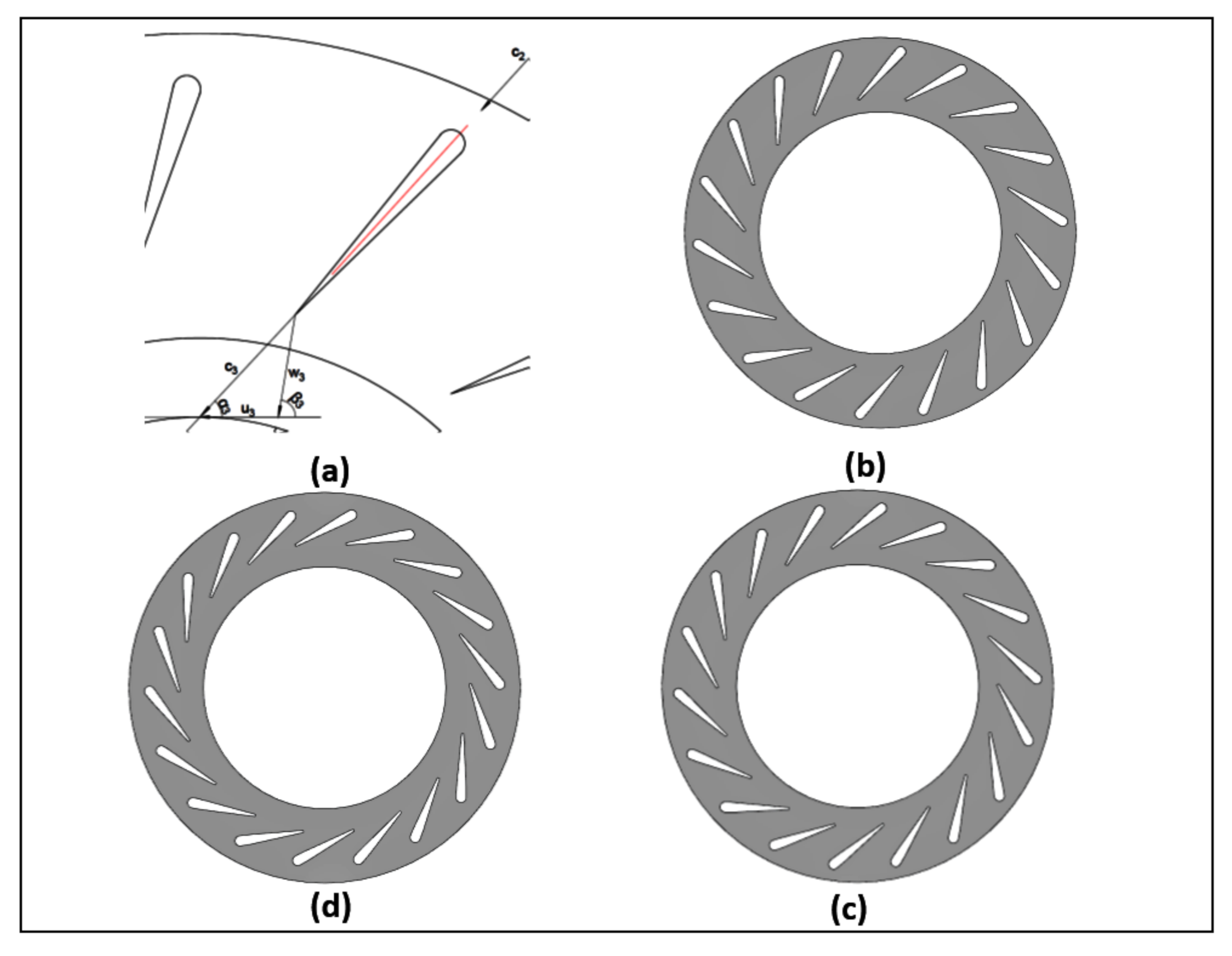
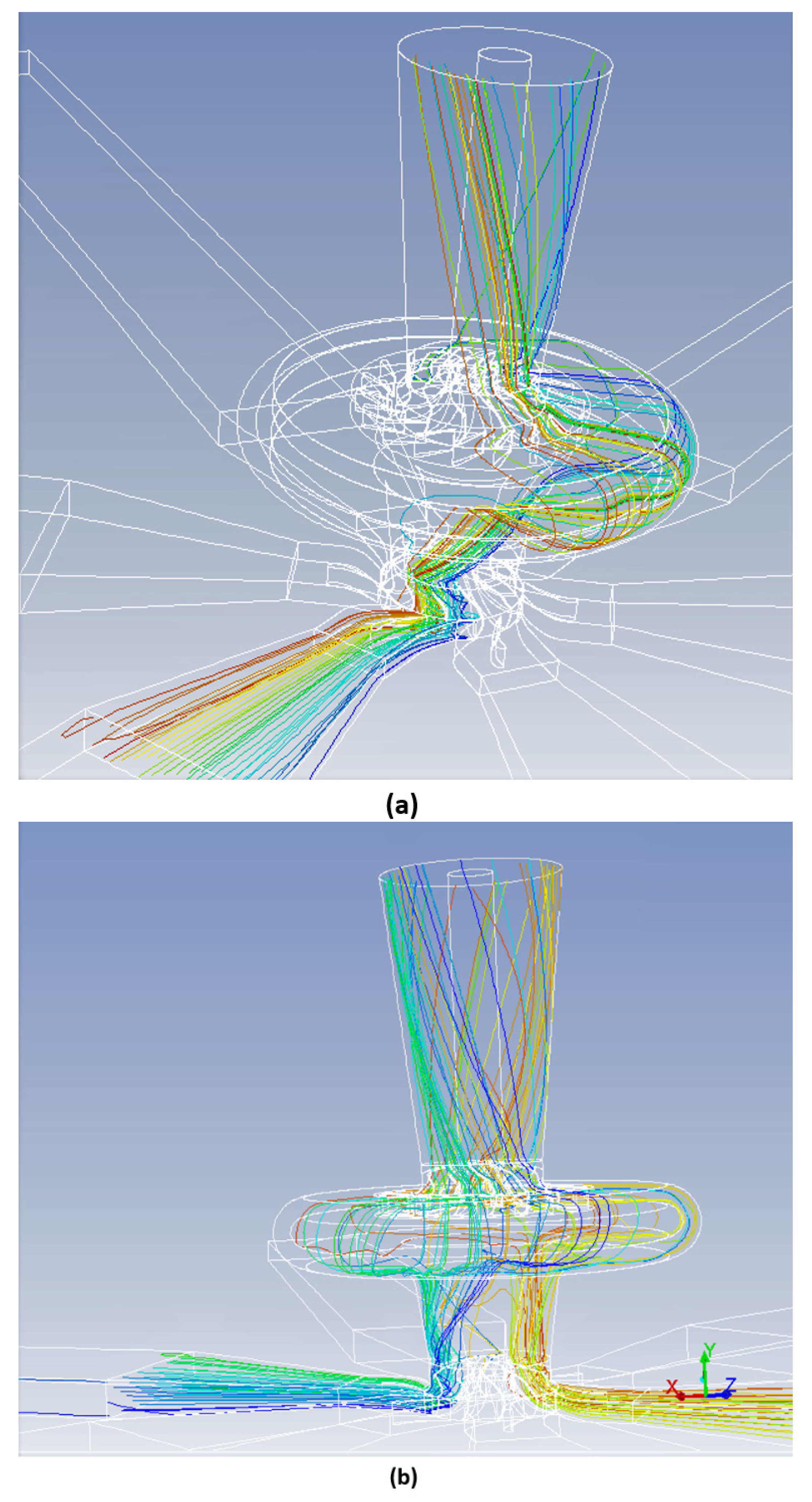
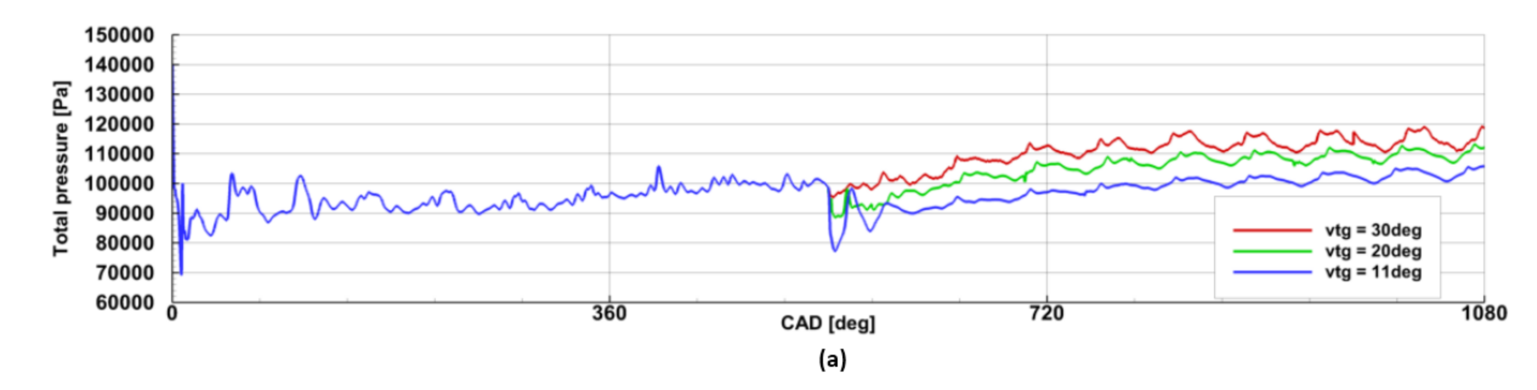
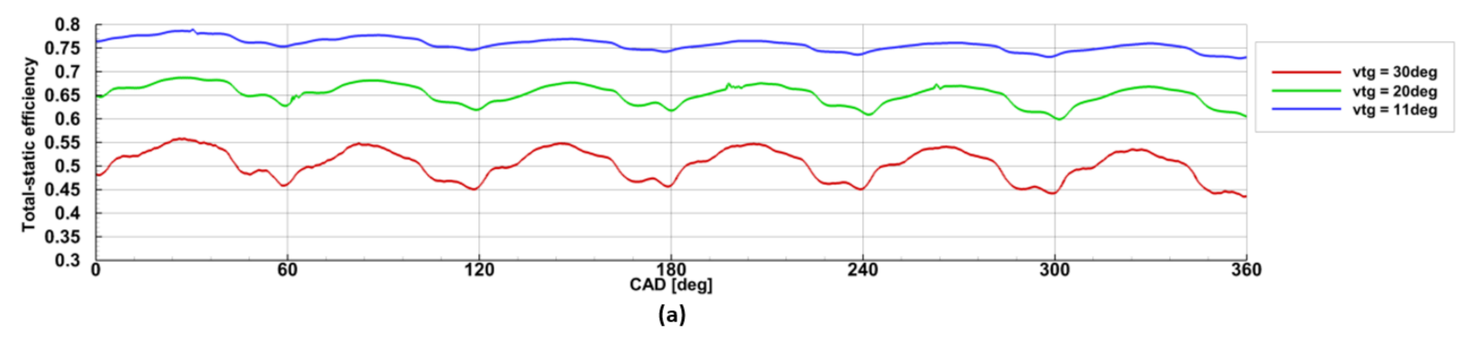
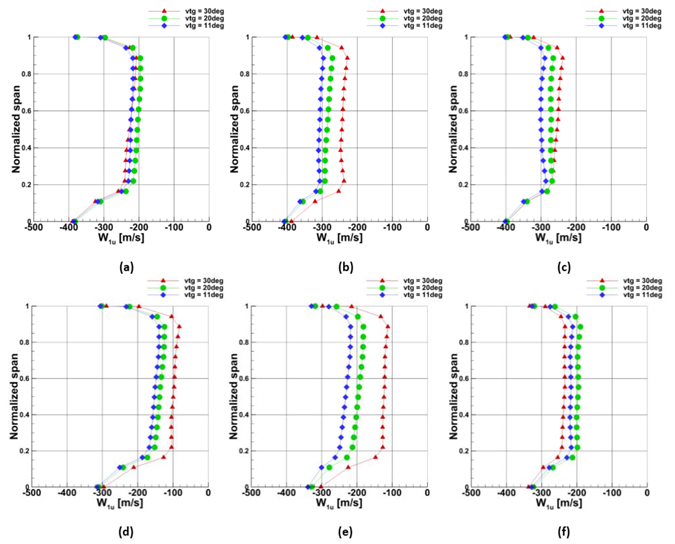
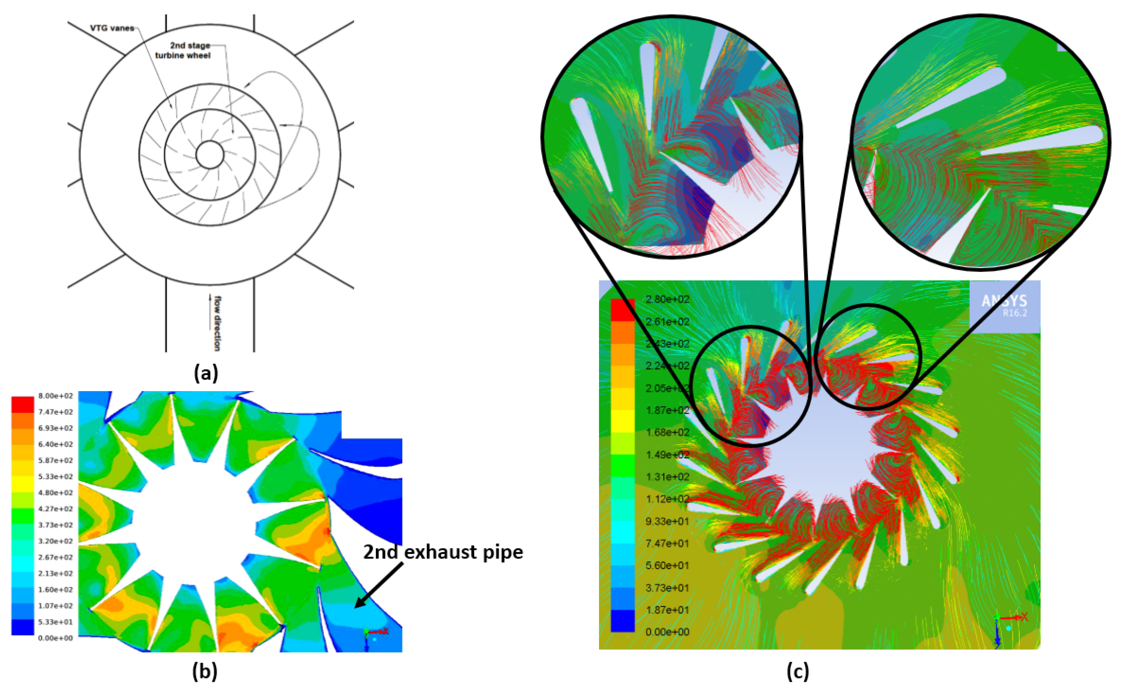
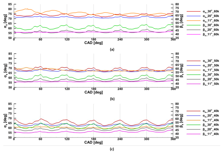
6.2. Flow at the VTG Nozzle Vanes

Figure 34 shows the complex flow pattern of the exhaust gases from the exhaust pipe to the VTG vanes.

According to Figure 14, the exhaust gases enter the VTG vane domain at the 90° direction to the previous direction in the exhaust pipe. Such a situation illustrates Figure 34a. Figure 34b shows that the exhaust gases enter the turbine tough the exhaust pipe 2. Furthermore, Figure 34c shows that those exhaust gases enter onto the VTG vanes at the angle of 80–120° to the previous direction in the exhaust pipe. The VTG vane domain was supplied at a quarter of its circumference.

Moreover, the zoomed regions in Figure 34c show that at the 120°, the pathlines of the exhaust gases are not aligned with the VTG vanes. The exhaust gases were flowing in the perpendicular direction to the vane pressure surface. On the other hand, the flow at the 80° was perfectly aligned with the vane position. Such phenomenon occurred in every position of the VTG vane and every turbine speed. It can be said that the flow path of the exhaust gases from the exhaust pipes to the VTG vanes is very complex. The exhaust gas direction changes rapidly after the 1st stage turbine wheel, which might create a vortex in the inter-stage pipes.

Figure 35 shows the absolute and relative angles at the outlet from the 2nd stage rotor at the three different turbine speeds.

The absolute angle greatly depended on the turbine speed. Thus, with the increase of the turbine speed, the absolute angle increased, as shown in Figure 36a.

The absolute velocity was closer to the axial direction at the turbine outlet for higher turbine speeds. Only minor changes of the outlet relative angle were observed. Figure 36b–d clearly show that the velocity pathlines are closer to the axial direction for 60,000 rpm. This means that the lowest energy losses at the turbine outlet occurred at 60,000 rpm.

7. Conclusions

This research was carried out to investigate the behavior of the two-stage turbine system with three different positions of the VTG vanes. The model had a unique inlet configuration which consisted of six equally placed inlets, which connected each of the six cylinders to the 1st stage rotor. Such an approach aimed to eliminate the interference of the exhaust pulses coming from adjacent pipes [29]. The Ansys Fluent software was used for transient turbomachinery flow simulations. The transient simulations with the sliding mesh approach allowed us to obtain instantaneous flow parameters at the interfaces connecting rotary (turbine wheel) and non-rotary domains. The three different VTG positions and the three different turbine speeds provided a great deal of valuable data. The simulated model of the two-stage turbine system was positively validated against the experimental data. Three revolutions of the crankshaft were performed to meet the required pressure changes in each exhaust pipe.

It was found out that the 1st stage rotor operates similarly to the typical scroll turbine. The 1st stage rotor is constantly supplied with exhaust gases due to coordinated changes of the pressure at the rotor inlet. The inlet pressure changed in a quasi-constant manner.

The in-depth analysis of the results showed a unique behavior of the 1st and 2nd stage rotors. With the increase of the turbine speed, the outlet temperature of the 1st stage rotor increased while the outlet temperature of the 2nd stage rotor decreased. Moreover, with the closure of the VTG vane, the outlet pressure of the 1st stage rotor increased, while the outlet pressure of the 2nd stage rotor decreased. The authors assumed that the closure on the VTG vane caused increased backpressure, which deteriorated the performance of the 1st stage rotor. Such a phenomenon affected the efficiency of both rotors. With the increase of the turbine speed, the efficiency of the 1st stage rotor decreased.

On the other hand, the efficiency of the 2nd stage rotor increased with the increase of the turbine speed. However, the average efficiency drop for the 1st stage rotor was 5%, while the efficiency increase for the 2nd stage rotor was 10%. That is why the 2nd stage rotor’s efficiency increase of the 2nd stage rotor balances the efficiency drop of the 1st stage rotor. It was also found that the position of the VTG had less influence on the efficiency of the 1st stage rotor than on the 2nd stage rotor. The maximal efficiency of the 2nd stage rotor was 75% for 60,000 rpm and 11° VTG position.

The authors investigated the flow parameters at the outlet from the 1st stage nozzle vane against the vane height. The parameters were monitored at the three control points: the maximal mass-flow rate, the medium mass-flow rate, and the minimal mass-flow rate.

It was found that the pressure increased with the increase of the turbine speed and with the closure of the VTG vane. Such phenomenon was observed for the temperature changes. The analysis of the velocity parameters allowed to conclude that the optimal flow parameters were obtained in the mid-span of the nozzle vane at the maximal mass-flow rate and low turbine speed (40,000 rpm). In such a configuration, the relative angle of the relative velocity W₁ is almost 90°. It provides a low incidence angle which is crucial to avoid pressure losses in the turbine inner-blade region.

The flow analysis of the exhaust gases through the VTG vanes was also investigated. The flow analysis showed that the exhaust gasses enter into the VTG vanes at the angle of 80–120° to the previous direction in the exhaust pipe. The exhaust gases enter the VTG section almost at the perpendicular direction to the vane pressure surface at the high flow angle. The streamlines of exhaust gases are perfectly aligned with the nozzle vanes at the lower flow angle.

With the increase of the turbine speed, the energy losses at the turbine outlet decreased as the absolute velocity was closer to the axial direction.

The highest average efficiency of the two-stage turbine system was 60% at 60,000 rpm with the 11° VTG position, which makes it a promising competitor for the modern scroll turbochargers. However, a direct comparison cannot be made as the compression work is not included in those calculations. The key feature of such a system is the turbine’s configuration inlet, which eliminates the interference of the pressure waves from the adjacent exhaust pipes. Such a feature eliminates the need for scrolled housing. More than one scroll turbocharger has to be installed for the multicylinder engine, which significantly complicates the exhaust system. The configuration of the two-stage turbine system makes it easier to adapt for multicylinder engines. In the future, such a two-stage system it intended to be manufactured and installed in a two-stroke, six-cylinder OP engine. Such an engine is being developed at the Warsaw University of Technology.

References

1. Thomas, A.; Samuel, J.; Ramesh, A. Mean-Line Modelling of a Variable Geometry Turbocharger (VGT) and Prediction of the Engine-Turbocharger Coupled Performance. In Proceedings of the ASME 2017 Gas Turbine India Conference, Bangalore, India, 7–8 December 2017. [Google Scholar]
2. Erik, T.; Flora, C.; Maria, R.J.; Igor, I. Fully Automated Multidisciplinary Design Optimization of a Variable Speed Turbine. In Proceedings of the 30th IAHR Symposium on Hydraulic Machinery and Systems (IAHR 2020), Lausanne, Switzerland, 21–26 March 2020. [Google Scholar]
3. Ponsankar, S.; Bikram, R.; Anshul, T. Turbocharger Lag Mitigation System. In Proceedings of the International Conference on Advances in Renewable and Sustainable Energy Systems (ICARSES 2020), Chennai, India, 3–5 December 2020. [Google Scholar]
4. Tong, Z.; Cheng, Z.; Tong, S. Preliminary Design of Multistage Radial Turbines Based on Rotor Loss Characteristics under Variable Operating Conditions. Energies 2019, 12, 2550. [Google Scholar] [CrossRef] [Green Version]
5. Lauriau, P.T.; Binder, N.; Cros, S.; Roumeas, M.; Carbonneau, X. Preliminary Design Considerations for Variable Geometry Radial Turbines with Multi-Points Specifications. Int. J. Turbomach. Propuls. Power 2018, 3, 22. [Google Scholar] [CrossRef] [Green Version]
6. Panneerselvam, S.; Vijayaragavan, M. Performance Analysis of Variable Geometry Turbocharged CI Engine. In Proceedings of the 2nd International conference on Advances in Mechanical Engineering (ICAME 2018), Kattankulathur, India, 22–24 March 2018. [Google Scholar]
7. Zamboni, G. A Study on Combustion Parameters in an Automotive Turbocharged Diesel Engine. Energies 2018, 11, 2531. [Google Scholar] [CrossRef] [Green Version]
8. Zamboni, G.; Moggia, S.; Capobianco, M. Effects of a Dual-Loop Exhaust Gas Recirculation System and Variable Nozzle Turbine Control on the Operating Parameters of an Automotive Diesel Engine. Energies 2017, 10, 47. [Google Scholar] [CrossRef] [Green Version]
9. Binder, N.; Le Guyader, S.; Carbonneau, X. Analysis of the Variable Geometry Effect in Radial Turbines. ASME J. Turbomach. 2012, 134, 1–9. [Google Scholar] [CrossRef] [Green Version]
10. Ricardo, M.B. Variable Geometry Mixed Flow Turbine for Turbochargers: An Experimental Study. Int. J. Fluid Mach. Syst. 2008, 1, 155–168. [Google Scholar] [CrossRef] [Green Version]
11. Wu, C.; Song, K.; Li, S.; Xie, H. Impact of Electrically Assisted Turbocharger on the Intake Oxygen Concentration and Its Disturbance Rejection Control for a Heavy-duty Diesel Engine. Energies 2019, 12, 3014. [Google Scholar] [CrossRef] [Green Version]
12. Pesiridis, A.; Saccomanno, A.; Tuccillo, R.; Capobianco, A. Conceptual Design of a Variable Geometry, Axial Flow Turbocharger Turbine. SAE Tech. Paper 2017, 1–16. [Google Scholar] [CrossRef]
13. Fayez, S.A.; Salah, L.; Adeel, M.; Mohammed, E.B. Estimation of Exhaust Gas Aerodynamic Force on the Variable Geometry Turbocharger Actuator: 1D Flow Model Approach. Energy Convers. Manag. 2014, 84, 436–447. [Google Scholar] [CrossRef]
14. Kumar, P.; Zhang, Y.; Traver, M.; Watson, J. Tailored Air-Handling System Development for Gasoline Compression Ignition in a Heavy-Duty Diesel Engine. Front. Mech. Eng. 2021, 7, 6. [Google Scholar] [CrossRef]
15. Thomas, A.; Samuel, J.J.; Pramod, M.P.; Ramesh, A.; Murugesan, R.; Kumarasamy, A. Simulation of a Diesel Engine with Variable Geometry Turbocharger and Parametric Study of Variable Vane Position on Engine Performance. Def. Sci. J. 2017, 67, 375–381. [Google Scholar] [CrossRef] [Green Version]
16. Vítek, O.; Macek, J.; Polášek, M. New Approach to Turbocharger Optimization using 1-D Simulation Tools. SAE Tech. Paper 2006, 1–17. [Google Scholar] [CrossRef]
17. Bharath, A.; Reitz, R.; Rutland, C. Impact of Active Control Turbocharging on the Fuel Economy and Emissions of a Light-Duty Reactivity Controlled Compression Ignition Engine: A Simulation Study. Front. Mech. Eng. 2021, 7, 8. [Google Scholar] [CrossRef]
18. Hu, B.; Li, J.; Li, S.; Yang, J. A Hybrid End-to-End Control Strategy Combining Dueling Deep Q-network and PID for Transient Boost Control of a Diesel Engine with Variable Geometry Turbocharger and Cooled EGR. Energies 2019, 12, 3739. [Google Scholar] [CrossRef] [Green Version]
19. Hu, B.; Yang, J.; Li, J.; Li, S.; Bai, H. Intelligent Control Strategy for Transient Response of a Variable Geometry Turbocharger System Based on Deep Reinforcement Learning. Processes 2019, 7, 601. [Google Scholar] [CrossRef] [Green Version]
20. Mirza, H.D.; Heath, W.P.; Apsley, J.M.; Forbes, J.R. Down-Speeding Diesel Engines with Two-Stage Turbochargers: Analysis And Control Considerations. Int. J. Eng. Res. 2020. [Google Scholar] [CrossRef]
21. Vincenzo, D.B.; Marelli, S.; Bozza, F.; Capobianco, M. 1D Simulation and Experimental Analysis of a Turbocharger Turbine for Automotive Engines under Steady and Unsteady Flow Conditions. Energy Procedia 2014, 45, 909–918. [Google Scholar] [CrossRef] [Green Version]
22. Pesyridis, A.; Vassil, B.; Padzillah, M.H.; Ricardo, M.B. A Comparison of Flow Control Devices for Variable Geometry Turbocharger Application. Int. J. Autom. Eng. Technol. 2014, 3, 1–21. [Google Scholar] [CrossRef] [Green Version]
23. Nonthakarn, P.; Ekpanyapong, M.; Nontakaew, U.; Bohez, E. Design and Optimization of an Integrated Turbo-Generator and Thermoelectric Generator for Vehicle Exhaust Electrical Energy Recovery. Energies 2019, 12, 3134. [Google Scholar] [CrossRef] [Green Version]
24. Osmić, M.; Delic, I. Determination of Flow Field in the Stator of the Variable Turbocharger. Mach. Technol. Mater. 2009, 2, 18–21. [Google Scholar]
25. Minasyan, A.; Bradshaw, J.; Pesyridis, A. Design and Performance Evaluation of an Axial Inflow Turbocharger Turbine. Energies 2018, 11, 278. [Google Scholar] [CrossRef] [Green Version]
26. Fulara, S.; Chmielewski, M.; Gieras, M. Variable Geometry in Miniature Gas Turbine for Improved Performance and Reduced Environmental Impact. Energies 2020, 13, 5230. [Google Scholar] [CrossRef]
27. Lei, H.; Hua, C. A Novel Design Method of Variable Geometry Turbine Nozzles for High Expansion Ratios. In Proceedings of the 17th International Symposium on Transport Phenomena and Dynamics of Rotating Machinery (ISROMAC2017), Maui, HI, USA, 16–21 December 2017. [Google Scholar]
28. Liu, J.; Qiao, W.Y.; Duan, W.H. Investigation of Unsteady Aerodynamic Excitation on Rotor Blade of Variable Geometry Turbine. Int. J. Rotating Mach. 2019, 1–13. [Google Scholar] [CrossRef]
29. Kozak, D.; Mazuro, P. Transient Simulation of the Six-Inlet, Two-Stage Radial Turbine under Pulse-Flow Conditions. Energies 2021, 14, 2043. [Google Scholar] [CrossRef]
30. Spalart, P.; Allmaras, S. A One-Equation Turbulence Model for Aerodynamic Flows. Rech. Aerosp. 1994, 1, 5–21. [Google Scholar]
Figure 1. The scanning process of the K44 turbine wheel.
Energies 14 05349 g001
Figure 2. (a) The isometric view at the numerical model showing six exhaust pipes, (b) the model cross-section, (c) the view at the 1st stage nozzle vane and the tip clearance domain [29].
Energies 14 05349 g002aEnergies 14 05349 g002b
Figure 3. Mesh generated on: (a) exhaust pipe, (b) 1st stage nozzle vane, (c) diffusor, (d) outlet, (e) 1st stage rotor.
Energies 14 05349 g003
Figure 4. (a) The inlet mas-flow rate and pressure-outlet boundary conditions, (b) boundary mass flow rate changes at the inlet to the exhaust pipes [29].
Energies 14 05349 g004
Figure 5. The positions of the VTG of the 2nd stage turbine wheel: (a) blade configuration (b) α3 = 30° deg, (c) α3 = 20° deg, (d) α3 = 11° deg.
Energies 14 05349 g005
Figure 6. The hexahedral mesh of the VTG domain at: (a) 30°, (b) 20°, (c) 11° opening.
Energies 14 05349 g006
Figure 7. The mass-average pressure changes during the single revolution of the crankshaft for different mesh density on: (a) exhaust pipe, (b) 1st stage rotor, (c) VTG vanes, (d) 2nd stage rotor [29].
Energies 14 05349 g007
Figure 8. The plot of the total pressure at the 1-st stage turbine inlet for the 30° VTG opening at: (a) 60,000 rpm, (b) 50,000 rpm, (c) 40,000 rpm turbine speed.
Energies 14 05349 g008
Figure 9. The plot of the total pressure at the 1-st stage turbine inlet for the 20° deg VTG opening at: (a) 60,000 rpm, (b) 50,000 rpm, (c) 40,000 rpm turbine speed.
Energies 14 05349 g009
Figure 10. The plot of the total pressure at the 1-st stage turbine inlet for the 11° VTG opening at: (a) 60,000 rpm, (b) 50,000 rpm, (c) 40,000 rpm turbine speed.
Energies 14 05349 g010
Figure 11. The pressure sensors: (a) Keller M8coolHB, (b) Kistler 4049A10.
Energies 14 05349 g011
Figure 12. Validation of the numerical model for (a) 60,000 rpm, (b) 50,000 rpm, (c) 40,000 rpm.
Energies 14 05349 g012
Figure 13. The residuals of the numerical simulation.
Energies 14 05349 g013
Figure 14. The pathlines from the: (a) single exhaust pipe, (b) two opposite exhaust pipes.
Energies 14 05349 g014
Figure 15. Example of the intersection of the pressure plots monitored at the Section 6.1 at the turbine speed of 40,000 rpm and 11° VTG opening.
Energies 14 05349 g015
Figure 16. The intersection of the pressure plot monitored at the Section 6.1 for the three different VTG opening at the turbine speed: (a) 60,000 rpm, (b) 50,000 rpm, (c) 40,000 rpm.
Energies 14 05349 g016
Figure 17. The outlet total pressure variation of the 1st stage rotor at the three different VTG openings for: (a) 60,000 rpm, (b) 50,000 rpm, (c) 40,000 rpm turbine speed.
Energies 14 05349 g017
Figure 18. The outlet total pressure variation of the 2nd stage rotor at the three different VTG openings for: (a) 60,000 rpm, (b) 50,000 rpm, (c) 40,000 rpm turbine speed.
Energies 14 05349 g018aEnergies 14 05349 g018b
Figure 19. The outlet total temperature variation at the 1st stage rotor at the three different VTG openings for: (a) 60,000 rpm, (b) 50,000 rpm, (c) 40,000 rpm.
Energies 14 05349 g019
Figure 20. The outlet total temperature variation at the 2nd stage rotor at the three different VTG openings for: (a) 60,000 rpm, (b) 50,000 rpm, (c) 40,000 rpm.
Energies 14 05349 g020
Figure 21. The averaged total-static efficiency of the 1st stage rotor at the three different VTG openings for: (a) 60,000 rpm, (b) 50,000 rpm, (c) 40,000 rpm during the single revolution of the crankshaft.
Energies 14 05349 g021
Figure 22. The averaged total-static efficiency of the 2nd stage rotor at the three different VTG openings for: (a) 60,000 rpm, (b) 50,000 rpm, (c) 40,000 rpm.
Energies 14 05349 g022aEnergies 14 05349 g022b
Figure 23. (a) The measuring points A, B, and C of the mass-flow rate at Section 6.1 of exhaust pipe 1, (b,c) the position of the control points at the trailing edge of the nozzle vane, (d) the velocity triangle at the outlet from the 1st stage nozzle vane of the exhaust pipe 1.
Energies 14 05349 g023aEnergies 14 05349 g023b
Figure 24. The plots of the total pressure measured behind the 1st stage nozzle vane against the blade height for: (ac) 60,000 rpm point A, B, C respectively, (df) 50,000 rpm point A, B, C respectively, (gi) 40,000 rpm point A, B, C respectively.
Energies 14 05349 g024
Figure 25. The plots of the total temperature measured behind the 1st stage nozzle vane against the blade height for: (ac) 60,000 rpm point A, B, C respectively, (df) 50,000 rpm point A, B, C respectively, (gi) 40,000 rpm point A, B, C respectively.
Energies 14 05349 g025aEnergies 14 05349 g025b
Figure 26. The plots of the absolute velocity C1 measured behind the 1st stage nozzle vane against the blade height for: (ac) 60,000 rpm point A, B, C respectively, (df) 50,000 rpm point A, B, C respectively, (gi) 40,000 rpm point A, B, C respectively.
Energies 14 05349 g026aEnergies 14 05349 g026b
Figure 27. The plots of the tangential component of the absolute velocity C1u measured behind the 1st stage nozzle vane against the blade height for: (ac) 60,000 rpm point A, B, C respectively, (df) 50,000 rpm point A, B, C respectively, (gi) 40,000 rpm point A, B, C respectively.
Energies 14 05349 g027aEnergies 14 05349 g027b
Figure 28. The plots of the relative velocity W1 measured behind the 1st stage nozzle vane against the blade height for: (ac) 60,000 rpm point A, B, C respectively, (df) 50,000 rpm point A, B, C respectively, (gi) 40,000 rpm point A, B, C respectively.
Energies 14 05349 g028aEnergies 14 05349 g028b
Figure 29. The plots of the tangential component of the relative velocity W1u measured behind the 1st stage nozzle vane against the blade height for: (ac) 60,000 rpm point A, B, C respectively, (df) 50,000 rpm point A, B, C respectively, (gi) 40,000 rpm point A, B, C respectively.
Energies 14 05349 g029aEnergies 14 05349 g029b
Figure 30. The plots of the absolute (α1) and relative (β1) angles measured behind the 1st stage nozzle vane against the blade height at 60,000 rpm for: (a) point A, (b) point B, (c) point C.
Energies 14 05349 g030
Figure 31. The plots of the absolute (α1) and relative (β1) angles measured behind the 1st stage nozzle vane against the blade height at 50,000 rpm for: (a) point A, (b) point B, (c) point C.
Energies 14 05349 g031
Figure 32. The plots of the absolute (α1) and relative (β1) angles measured behind the 1st stage nozzle vane against the blade height at 40,000 rpm for: (a) point A, (b) point B, (c) point C.
Energies 14 05349 g032aEnergies 14 05349 g032b
Figure 33. (a) The configuration of the outlet velocity triangles at the against the height of the 1st stage nozzle vane, the comparison of the velocity triangles at the outlet of the 1st stage nozzle vane at: (b) points A, B, and C, (c) at three different turbine speeds.
Energies 14 05349 g033
Figure 34. (a) A diagram of a flow path from the exhaust pipe to the VTG vanes, (b) the contours of the total pressure at the 1st stage turbine wheel during the flow from the exhaust pipe no 2, (c) the velocity pathlines at the VTG vanes during the flow from the exhaust pipe no 2.
Energies 14 05349 g034
Figure 35. The absolute and relative angle at the outlet from the 2nd stage rotor for: (a) 60,000 rpm, (b) 50,000 rpm, (c) 40,000 rpm turbine speed.
Energies 14 05349 g035
Figure 36. (a) Configuration of velocity triangles at the outlet from the 2nd stage rotor, (b) outlet velocity pathlines at 60,000 rpm, (c) outlet velocity pathlines at 50,000 rpm, (d) outlet velocity pathlines at 40,000 rpm.
Energies 14 05349 g036