
Real-Time HEV Energy Management Strategy Considering Road Congestion Based on Deep Reinforcement Learning


Abstract
:1. Introduction
2. Preliminaries
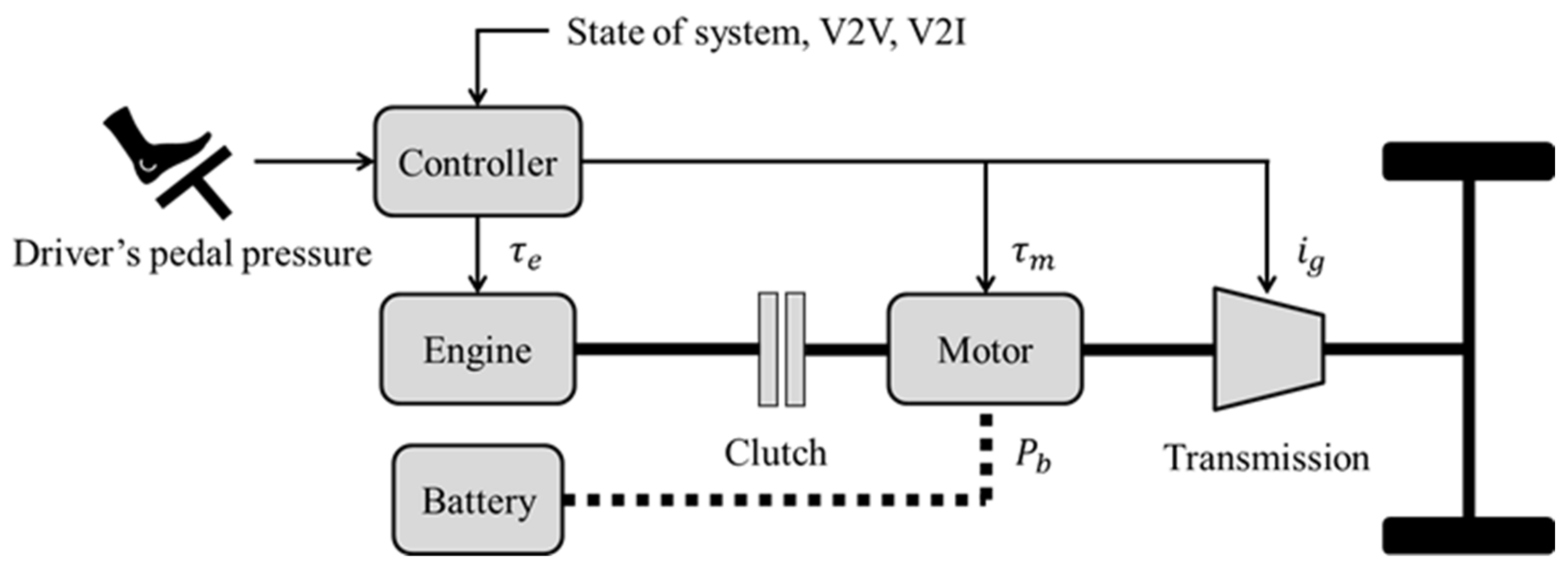
2.1. System Modeling
2.2. Problem Formulation
3. Control Design
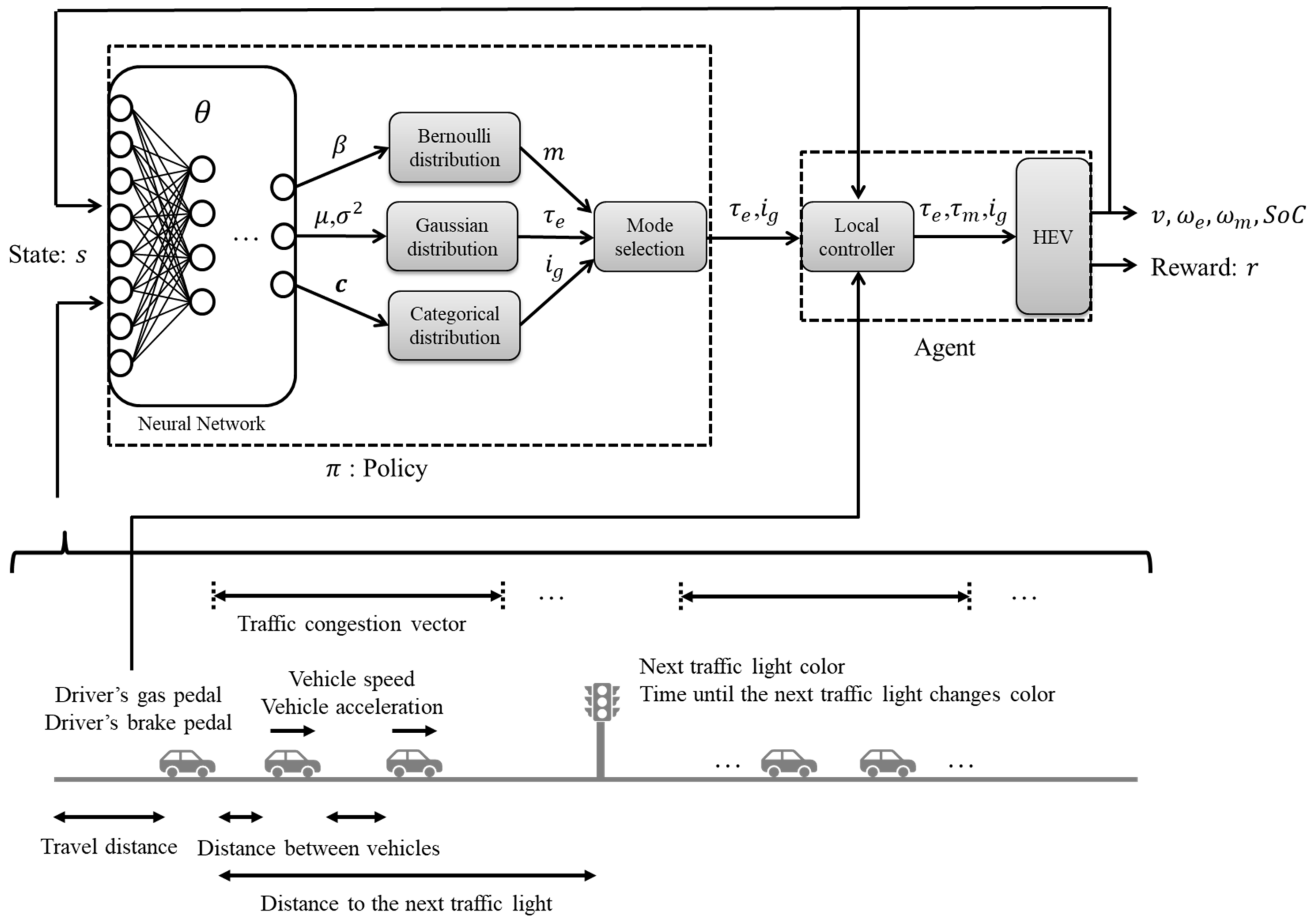
3.1. Overview
3.2. State
3.3. Policy Model
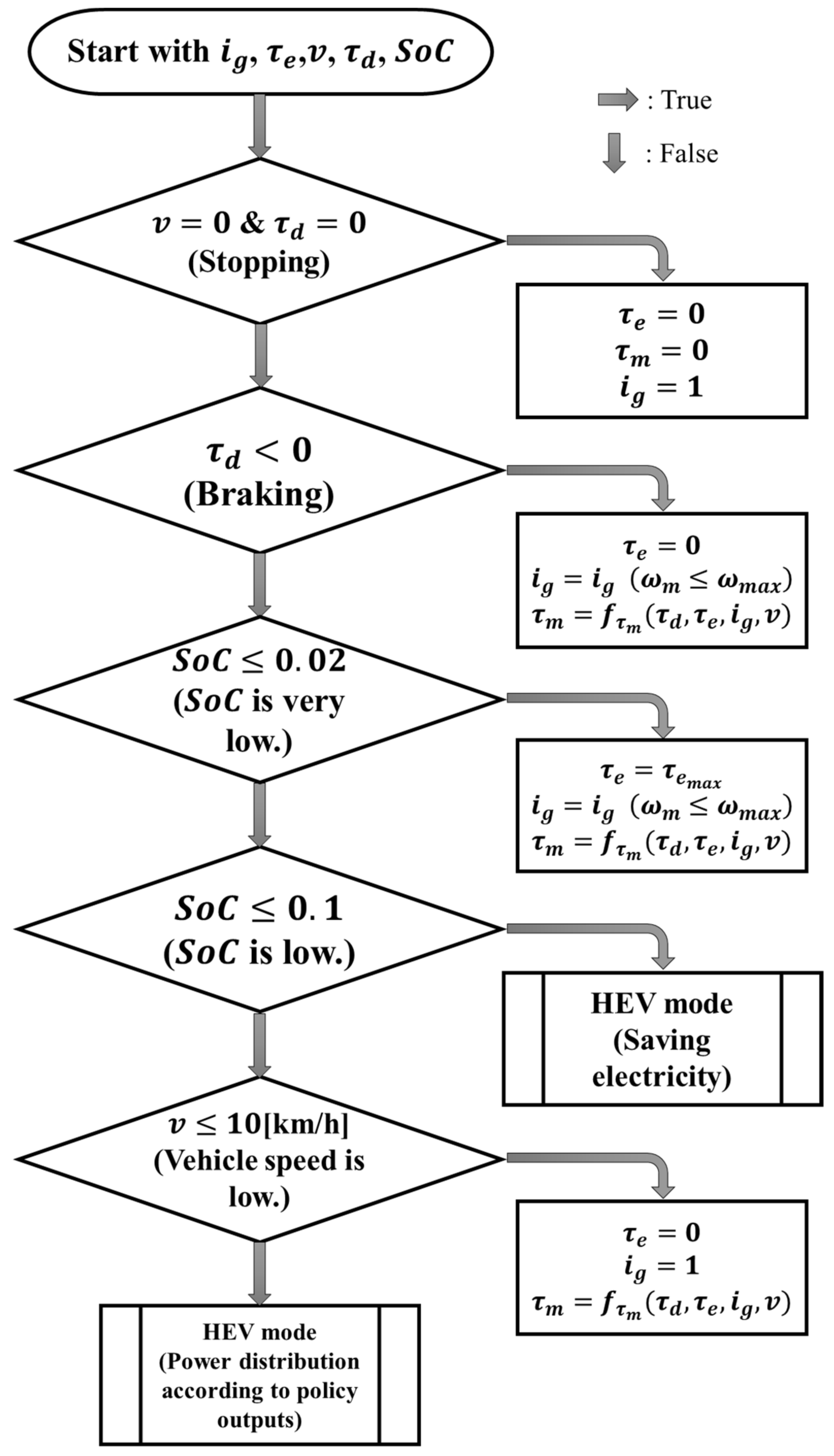
3.4. Local Controller
3.5. Proximal Policy Optimization
3.6. Generalized Advantage Estimator
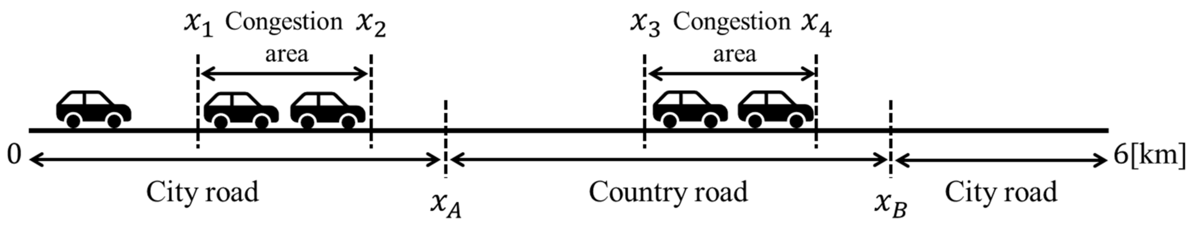
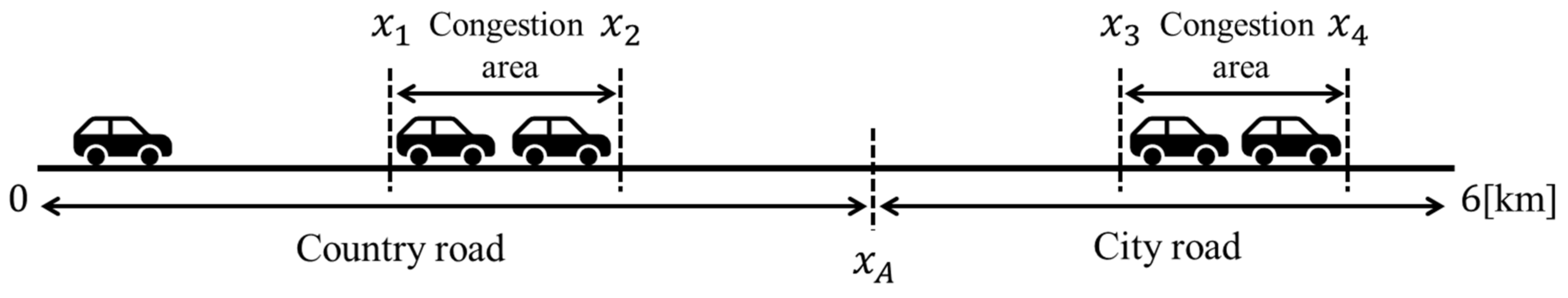
4. Simulation
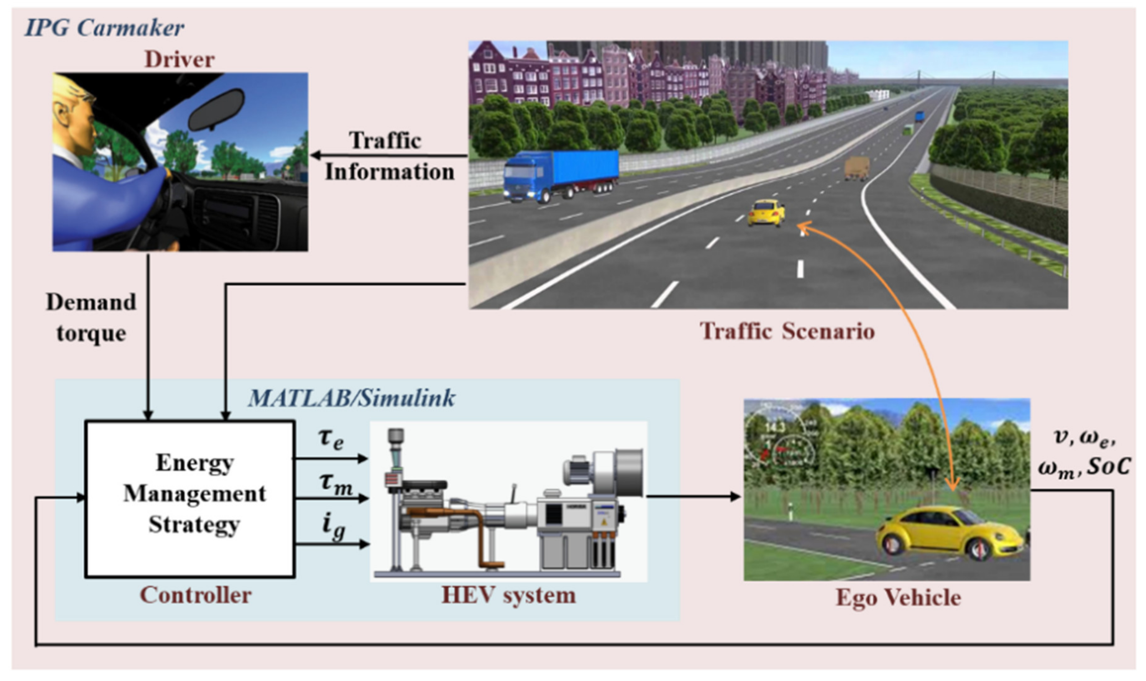
4.1. Overview
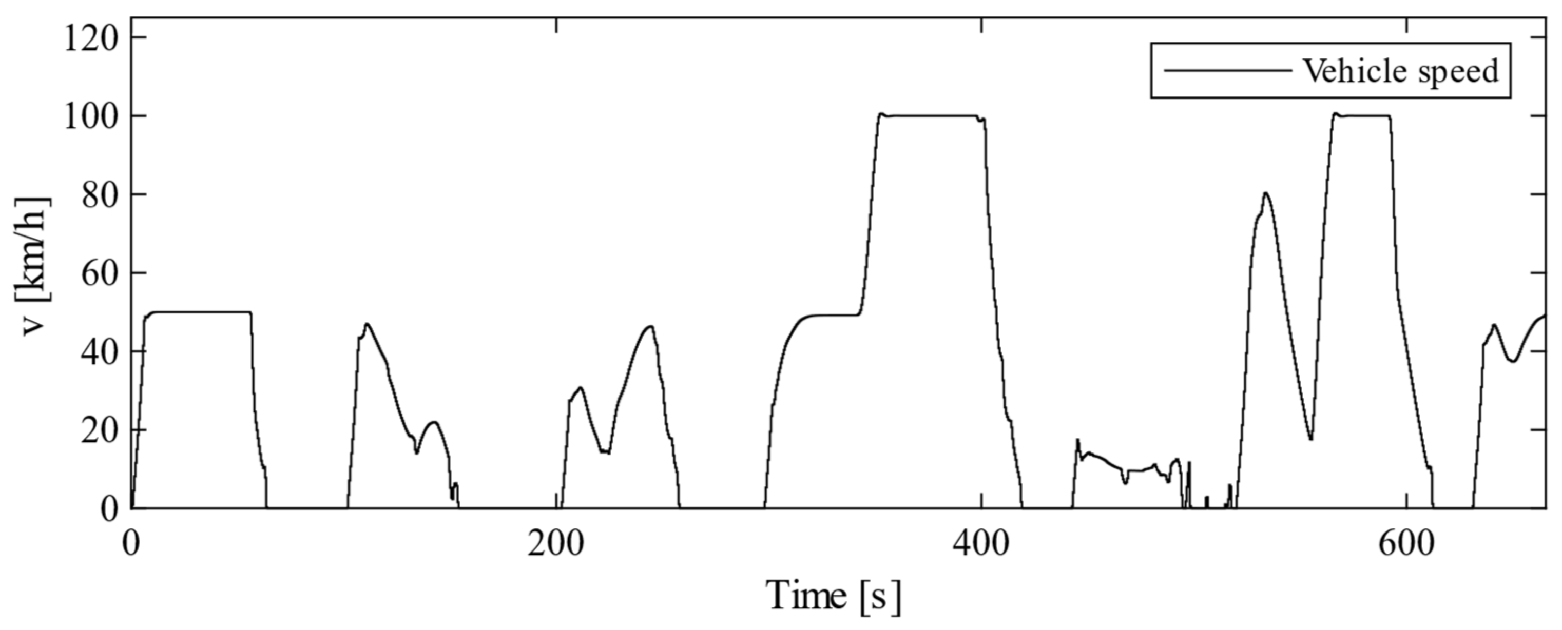
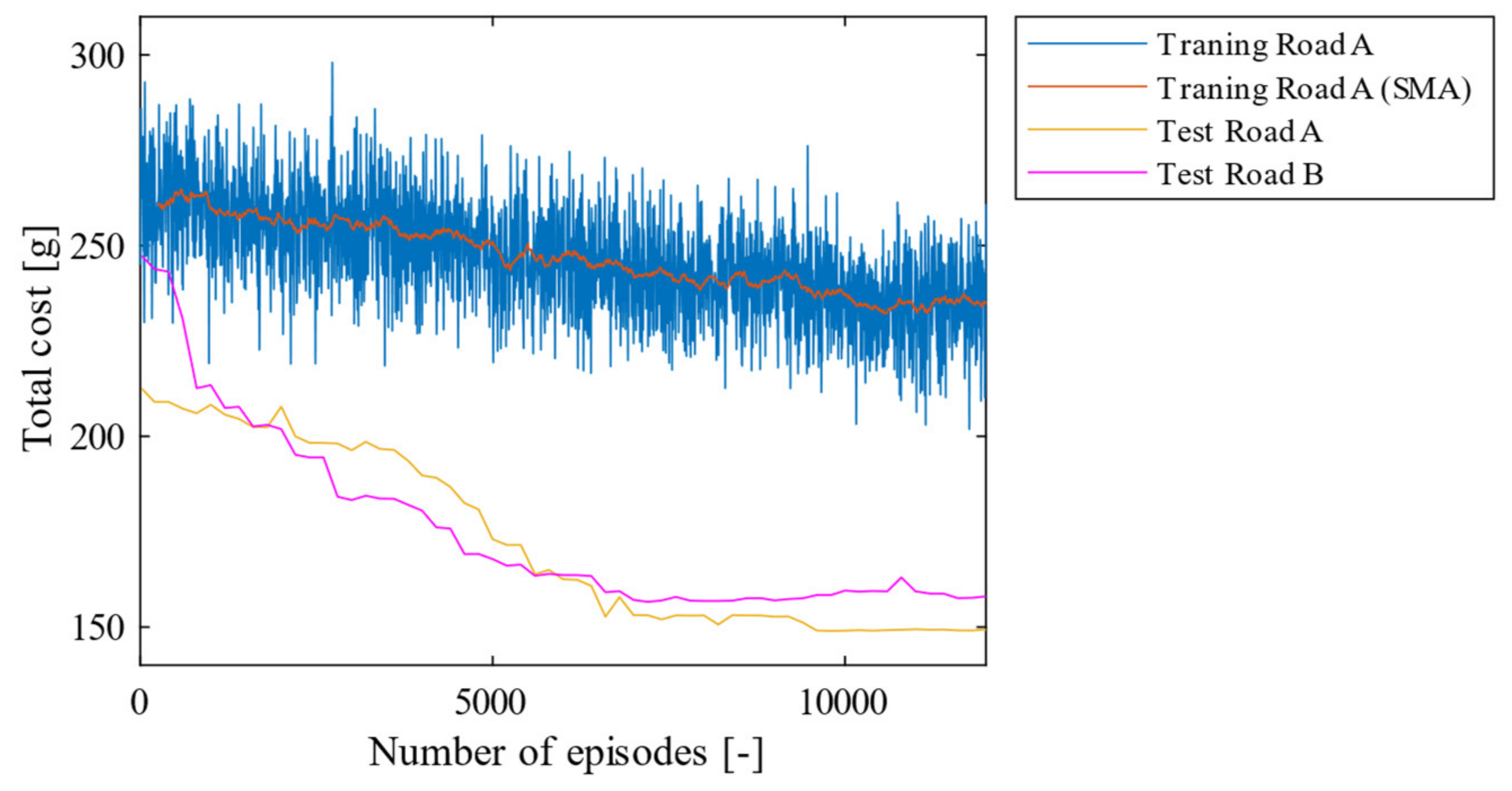
4.2. Simulation Results of the Proposed Method
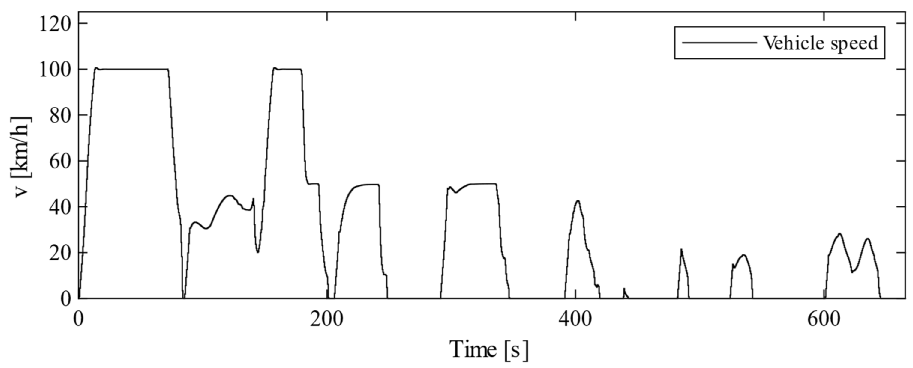
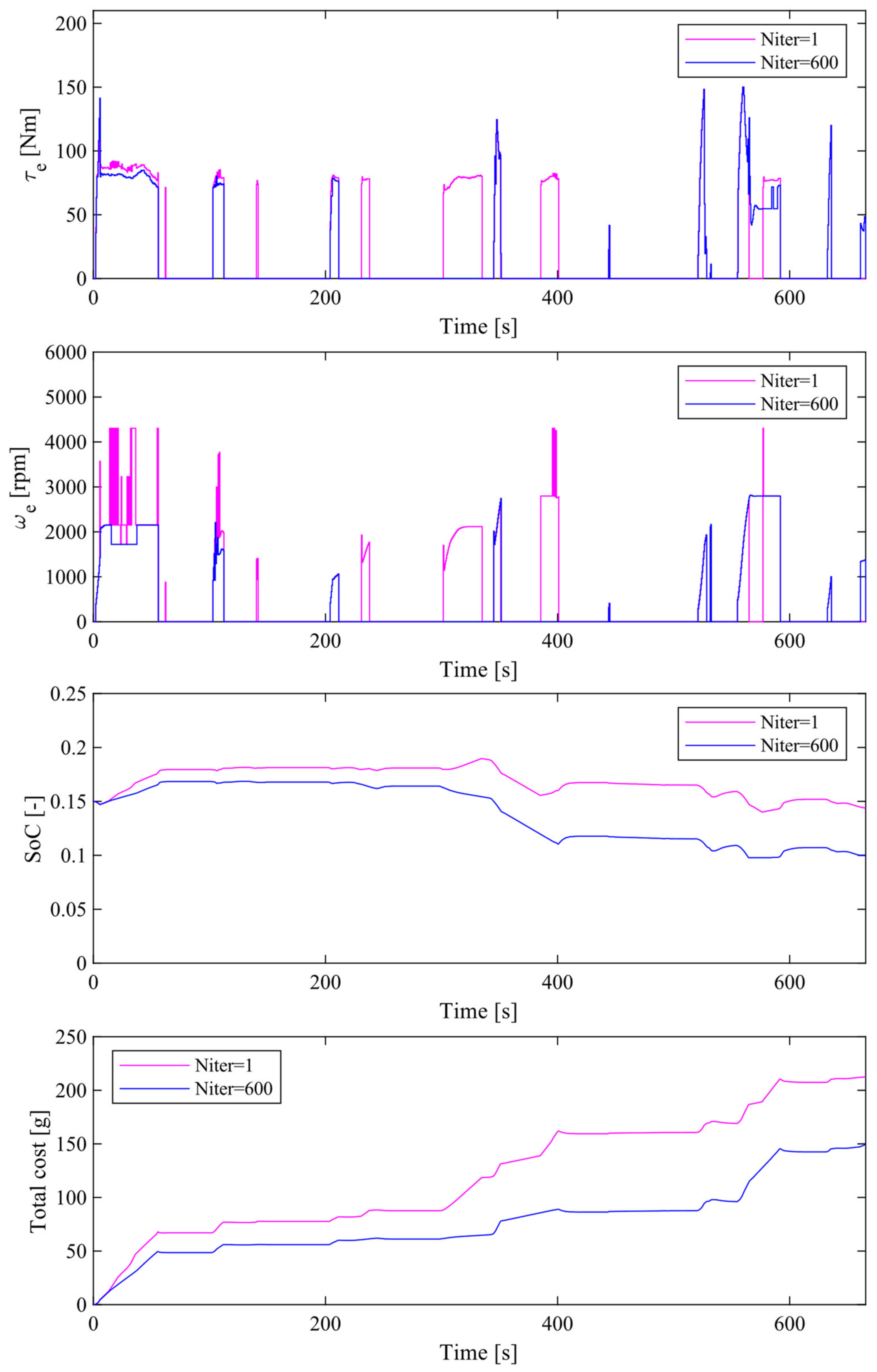
4.3. Simulation Results of the Proposed Method without Traffic Congestion Vector
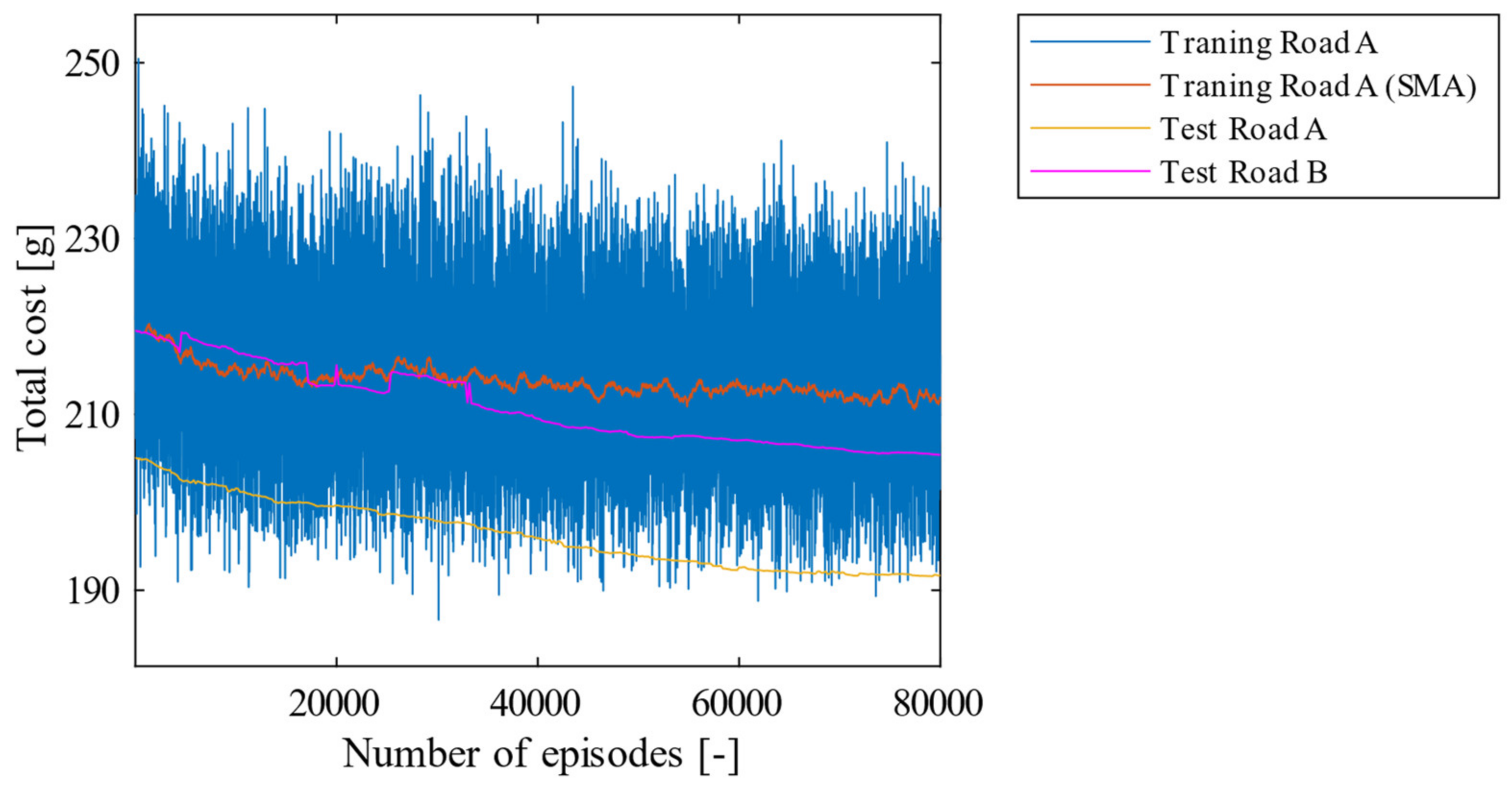
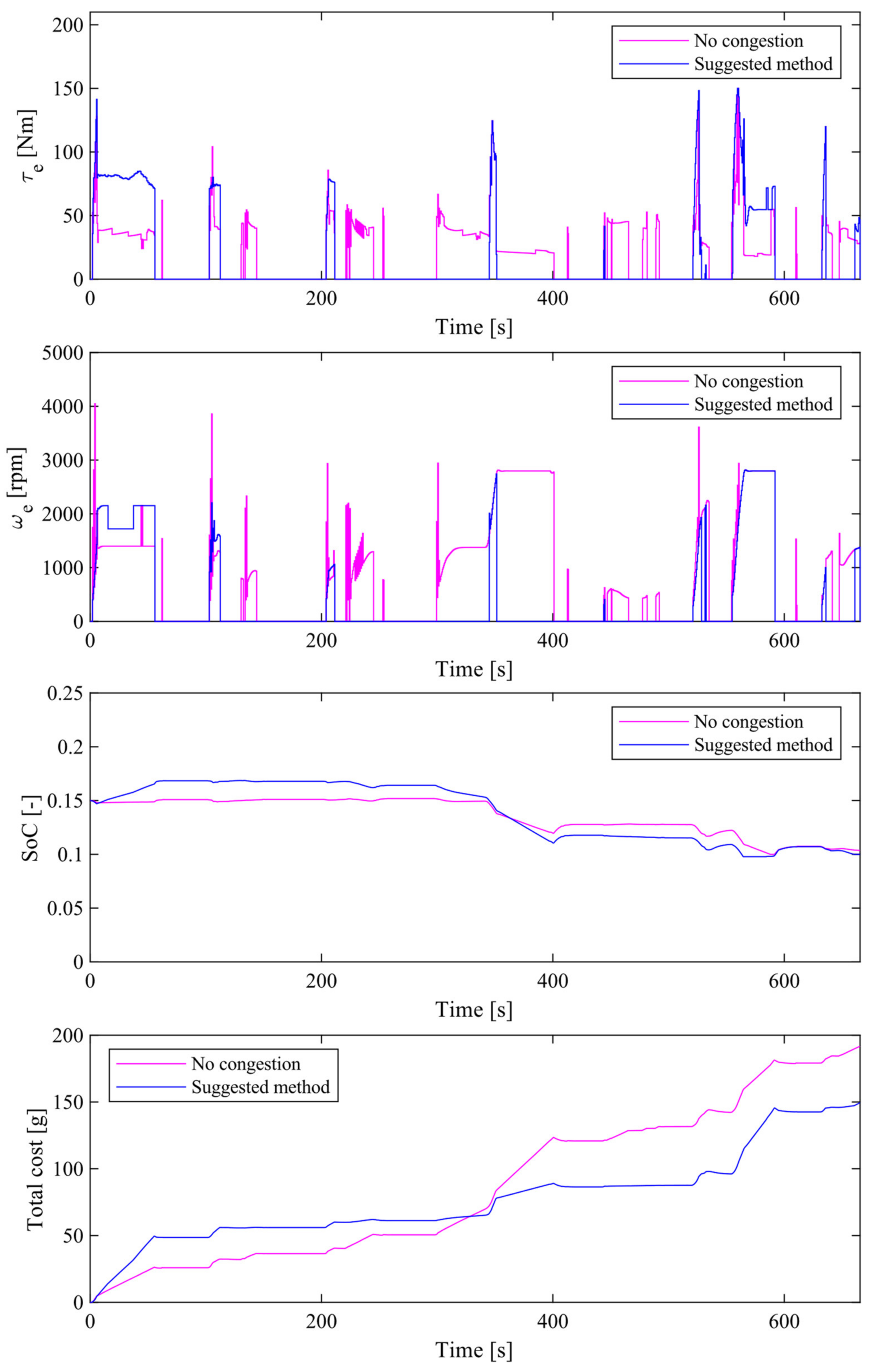
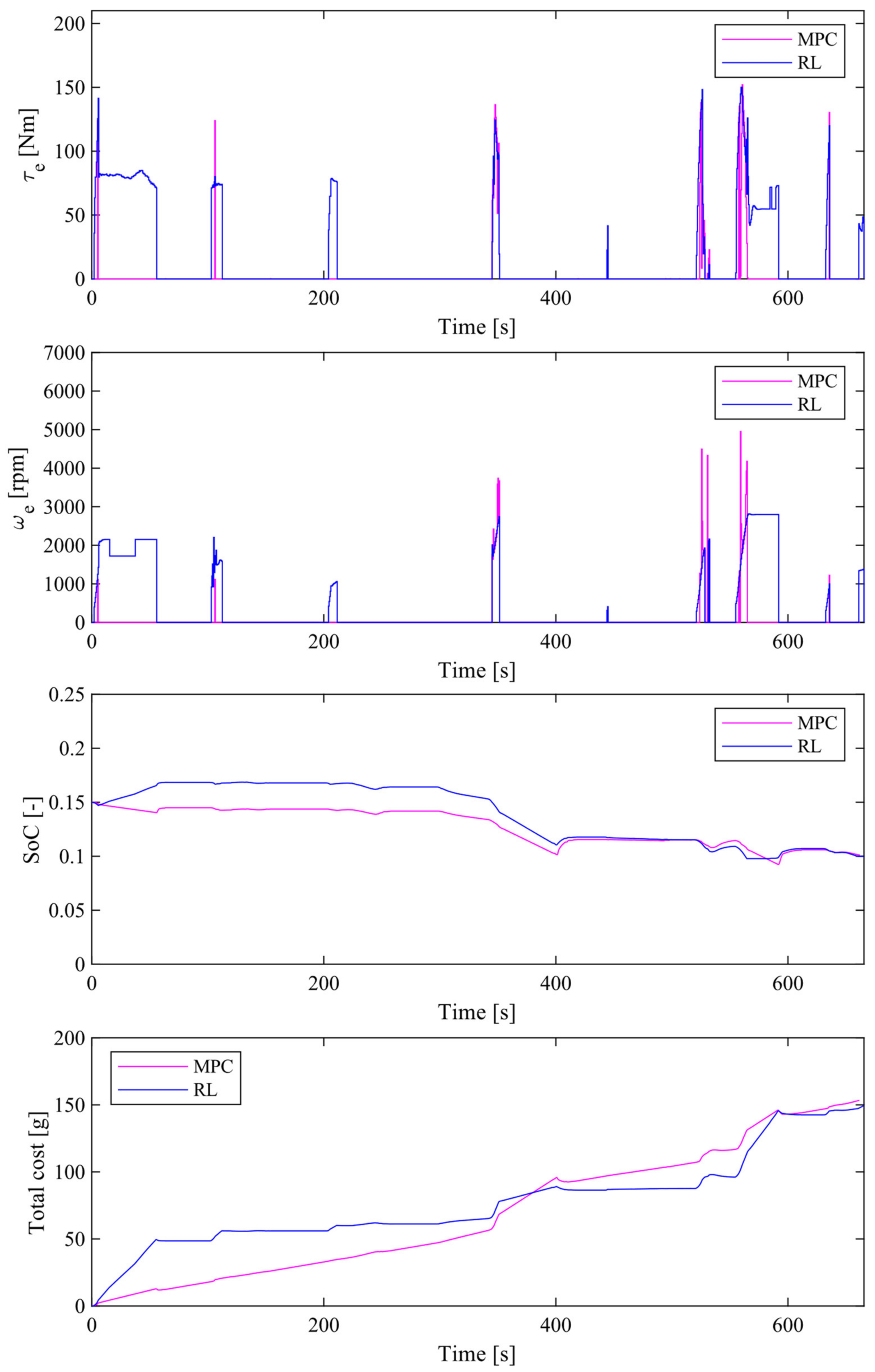
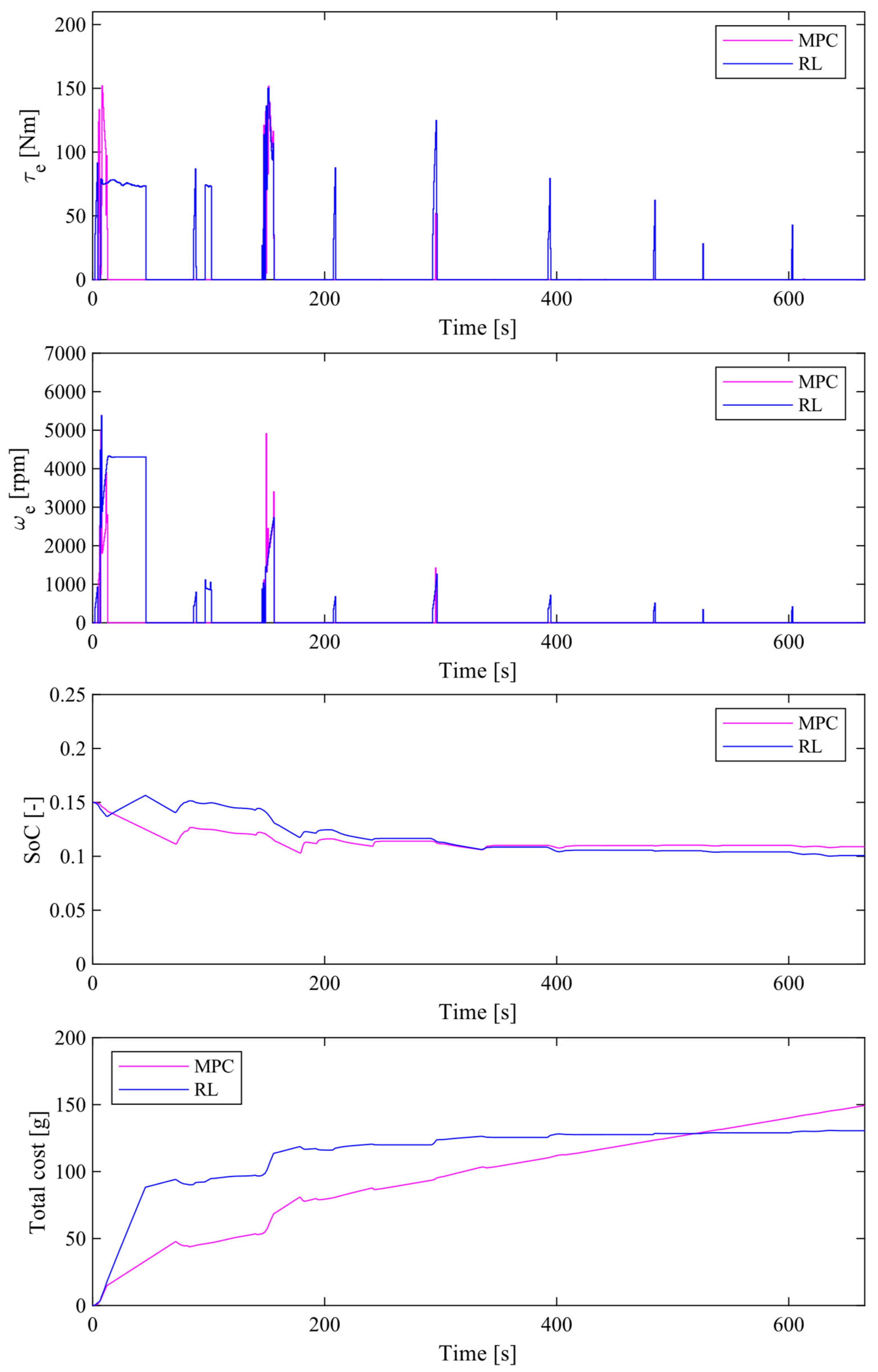
4.4. Comparison of Simulation Results between the Proposed Method and MPC
5. Conclusions
Author Contributions
Funding
Institutional Review Board Statement
Informed Consent Statement
Conflicts of Interest
References
- Hofman, T.; Steinbuch, M.; van Druten, R.M.; Serrarens, A.F.A. Rule-Based Equivalent Fuel Consumption Minimization Strategies for Hybrid Vehicles. In Proceedings of the 17th IFAC World Congress, Seoul, Korea, 6–11 June 2008; Volume 41, pp. 5652–5657. [Google Scholar] [CrossRef] [Green Version]
- Wang, R.; Lukic, S.M. Dynamic programming technique in hybrid electric vehicle optimization. In Proceedings of the 2012 IEEE International Electric Vehicle Conference, Greenville, SC, USA, 4–8 March 2012. [Google Scholar] [CrossRef]
- Borhan, H.; Vahidi, A.; Phillips, A.M.; Ming, L.; Kuang, I.; Kolmanovsky, V.; Di Cairano, S. MPC-based energy management of a power-split hybrid electric vehicle. IEEE Trans. Control Syst. Technol. 2012, 20, 593–603. [Google Scholar] [CrossRef]
- Xu, F.; Shen, T. Look-Ahead Prediction-Based Real-Time Optimal Energy Management for Connected HEVs. IEEE Trans. Veh. Technol. 2020, 69, 2537–2551. [Google Scholar] [CrossRef]
- Hu, J.; Shao, Y.; Sun, Z.; Wang, M.; Bared, J.; Huang, P. Integrated optimal eco-driving on rolling terrain for hybrid electric vehicle with vehicle-infrastructure communication. Transp. Res. Part C Emerg. Technol. 2016, 68, 228–244. [Google Scholar] [CrossRef]
- Zhang, B.; Zhang, J.; Xu, F.; Shen, T. Optimal control of power-split hybrid electric powertrains with minimization of energy consumption. Appl. Energy 2020, 266, 114873. [Google Scholar] [CrossRef]
- Schulman, J.; Wolski, F.; Dhariwal, P.; Radford, A.; Klimov, O. Proximal Policy Optimization Algorithms. arXiv 2017, arXiv:1707.06347. [Google Scholar]
- Schulman, J.; Levine, S.; Moritz, P.; Jordan, M.; Abbeel, P. Trust Region Policy Optimization. arXiv 2015, arXiv:1502.05477. [Google Scholar]
- Schulman, J.; Moritz, P.; Levine, S.; Jordan, M.; Abbeel, P. High-Dimensional Continuous Control Using Generalized Advantage Estimation. arXiv 2015, arXiv:1506.02438. [Google Scholar]
- Heess, N.; Dhruva, T.B.; Sriram, S.; Lemmon, J.; Merel, J.; Wayne, G.; Tassa, Y.; Erez, T.; Ziyu Wang, S.M.; Eslami, A.; et al. Emergence of Locomotion Behaviours in Rich Environments. arXiv 2017, arXiv:1707.02286. [Google Scholar]
- Mnih, V.; Puigdomenech Badia, A.; Mirza, M.; Alex Graves, L.T.P.; Harley, T.; Silver, D.; Kavukcuoglu, K. Asynchronous Methods for Deep Reinforcement Learning. arXiv 2016, arXiv:1602.01783. [Google Scholar]
- Martens, J.; Sutskever, I. Training deep and recurrent networks with hessian-free optimization. In Neural Networks: Tricks of the Trade; Springer: Berlin/Heidelberg, Germany, 2012; pp. 479–535. [Google Scholar] [CrossRef] [Green Version]
- Pascanu, R.; Bengio, Y. Revisiting Natural Gradient for Deep Networks. arXiv 2013, arXiv:1301.3584. [Google Scholar]
- Lillicrap, T.P.; Hunt, J.J.; Pritzel, A.; Heess, N.; Erez, T.; Tassa, Y.; Silver, D.; Wierstra, D. Continuous Control with Deep Reinforcement Learning. arXiv 2015, arXiv:1509.02971. [Google Scholar]
- Van Hasselt, H.; Guez, A.; Silver, D. Deep Reinforcement Learning with Double Q-Learning. arXiv 2016, arXiv:1509.06461. [Google Scholar]
- Schaul, T.; Quan, J.; Antonoglou, I.; Silver, D. Prioritized Experience Replay. arXiv 2016, arXiv:1511.05952. [Google Scholar]
- Hu, Y.; Li, W.; Xu, K.; Zahid, T.; Qin, F.; Li, C. Energy Management Strategy for a Hybrid Electric Vehicle Based on Deep Reinforcement Learning. Appl. Sci. 2018, 8, 187. [Google Scholar] [CrossRef] [Green Version]
- Liessner, R.; Schroer, C.; Dietermann, A.; Baker, B. Deep Reinforcement Learning for Advanced Energy Management of Hybrid Electric Vehicles. In Proceedings of the 10th International Conference on Agents and Artificial Intelligence, Madeira, Portugal, 16–18 January 2018. [Google Scholar] [CrossRef]
- Yang, C.; Zhou, C. An Energy Management Strategy of Hybrid Electric Vehicles based on Deep Reinforcement Learning. Int. J. Eng. Adv. Res. Technol. 2019, 5, 1–4. [Google Scholar]
- Lee, H.; Song, C.; Kim, N.; Cha, S.W. Comparative Analysis of Energy Management Strategies for HEV: Dynamic Programming and Reinforcement Learning. IEEE Access 2020, 8, 67112–67123. [Google Scholar] [CrossRef]
- Liu, T.; Wang, B.; Tan, W.; Lu, S.; Yang, Y. Data-Driven Transferred Energy Management Strategy for Hybrid Electric Vehicles via Deep Reinforcement Learning. arXiv 2020, arXiv:2009.03289. [Google Scholar]
- Kingma, D.P.; Ba, J. Adam: A Method for Stochastic Optimization. arXiv 2014, arXiv:1412.6980. [Google Scholar]

| State: | Driver’s gas pedal pressure [−] |
| Driver’s brake pedal pressure [−] | |
| Vehicle speed (v) [] | |
| Engine speed () [rpm] | |
| Motor speed () [rpm] | |
| Battery charge rate () [−] | |
| Distance to the vehicle in front [m] | |
| Vehicle speed in front [] | |
| Vehicle acceleration in front [] | |
| Distance between the vehicle in front and two vehicles ahead [] | |
| Speed of two vehicles ahead [] | |
| Acceleration of two vehicles ahead [] | |
| Traffic congestion vector [−] | |
| Next traffic light color [−] | |
| Time until the color of next traffic light changes [] | |
| Distance to the next traffic light [] |
| Training data | Road A | 1700 | 5400 | 800 | 1200 | 4100 | 4700 |
| 2200 | 5500 | 1200 | 1700 | 4200 | 4800 | ||
| 2200 | 5300 | 1400 | 1800 | 3700 | 4200 | ||
| 1800 | 5300 | 900 | 1400 | 3700 | 4400 | ||
| 2000 | 5700 | 1100 | 1500 | 4500 | 5000 | ||
| Test data | Road A | 2000 | 5500 | 1000 | 1400 | 4000 | 4500 |
| Road B | 3500 | - | 2000 | 2600 | 5000 | 5400 | |
| Initial Value and Hyperparameter | Value |
|---|---|
| [s] | 0.5 |
| [km/h], [rpm], [rpm] | 0 |
| [%] | 15 |
| Number of hidden layers in the policy [−] | 2 |
| Number of hidden layers in the value function [−] | 2 |
| Number of units in the policy [−] | [64, 64] |
| Number of units in the value function [−] | [64, 32] |
| [−] | 363.09 |
| [Nm] | 150 |
| [−] | 30 |
| [−] | 0.9999 |
| [−] | 0.95 |
| Learning rate [−] | 3 × 10⁻⁸ |
| [−] | 0.2 |
| [−] | 20 |
| [−] | 128 |
| [−] | 10 |
| Road Type | Total Cost [g] | Distance Per Liter [km/ℓ] |
|---|---|---|
| Test: Road A | 149.34 | 30.13 |
| Test: Road B | 158.04 | 28.47 |
| Road Type | Total Cost [g] | Distance per Liter [km/ℓ] |
|---|---|---|
| Test: Road A | 191.71 | 23.47 |
| Test: Road B | 205.41 | 21.91 |
| Road Type | Total Cost [g] | Distance per Liter [km/ℓ] |
|---|---|---|
| Test: Road A | 155.01 | 29.03 |
| Test: Road B | 172.93 | 26.02 |
Publisher’s Note: MDPI stays neutral with regard to jurisdictional claims in published maps and institutional affiliations. |
© 2021 by the authors. Licensee MDPI, Basel, Switzerland. This article is an open access article distributed under the terms and conditions of the Creative Commons Attribution (CC BY) license (https://creativecommons.org/licenses/by/4.0/).
Share and Cite
Inuzuka, S.; Zhang, B.; Shen, T. Real-Time HEV Energy Management Strategy Considering Road Congestion Based on Deep Reinforcement Learning. Energies 2021, 14, 5270. https://doi.org/10.3390/en14175270
Inuzuka S, Zhang B, Shen T. Real-Time HEV Energy Management Strategy Considering Road Congestion Based on Deep Reinforcement Learning. Energies. 2021; 14(17):5270. https://doi.org/10.3390/en14175270
Chicago/Turabian StyleInuzuka, Shota, Bo Zhang, and Tielong Shen. 2021. "Real-Time HEV Energy Management Strategy Considering Road Congestion Based on Deep Reinforcement Learning" Energies 14, no. 17: 5270. https://doi.org/10.3390/en14175270
APA StyleInuzuka, S., Zhang, B., & Shen, T. (2021). Real-Time HEV Energy Management Strategy Considering Road Congestion Based on Deep Reinforcement Learning. Energies, 14(17), 5270. https://doi.org/10.3390/en14175270