Article

County Clustering with Bioenergy as Flexible Power Unit in a Renewable Energy System

1
Chair for Wind Power Drives, RWTH Aachen University, Campus-Boulevard 61, 52074 Aachen, Germany
2
Institute for Machine Elements and System Engineering, RWTH Aachen University, Schinkelstraße 10, 52062 Aachen, Germany
*
Author to whom correspondence should be addressed.
Energies 2021, 14(17), 5227; https://doi.org/10.3390/en14175227
Submission received: 27 July 2021 / Revised: 11 August 2021 / Accepted: 16 August 2021 / Published: 24 August 2021

Abstract

:
The pressure on the energy sector to reduce greenhouse gas emissions is increasing. In the light of current greenhouse gas emissions in the energy sector, further expansion of renewable energy sources (RES) is inevitable to reduce emissions and reach the climate goals. This study aims at investigating structural characteristics of German counties regarding advantages for self-sufficient power systems based on RES. The modelling of the power sector based on RES is coupled with a cluster analysis in order to draw a large-scale conclusion on structural characteristics beneficial or obstructive for municipal energy systems. Ten clusters are identified with the Ward algorithm in a hierarchical-agglomerative method. The results underline a further need for RES expansion projects in order to close the gap between supply and demand. Only then, bioenergy can effectively balance the offset and support a truly self-sufficient local energy system. While the model results indicate that the majority of the counties are suitable for further expansion, this suitability is to be questioned in cluster 10. High population density is a critical characteristic, because with it come both a high demand and limited sites for further RES expansion projects.

1. Introduction

With the ratification of the Paris Agreement in 2016, the German government set the national greenhouse gas reduction goals to 80 to 95% compared to 1990 [1]. The Climate Change Act 2021 set those goals legally binding and aims at climate neutrality by 2045. The pressure on the energy sector above all sectors to reduce greenhouse gas emissions is increasing. With lignite & coal combustion being one of the main sources for greenhouse gases in the energy sector, further expansion of renewable energy sources (RES) is inevitable to reduce emissions and reach the climate goals [2]. With rapid extension of RES capacities and the mainly fluctuating feed-in patterns, the integration of power supply in the grid becomes a growing challenge. The need for energy system knowledge both on local and national level is increasing.
In rural areas with comparatively high RES potential, municipal energy systems are an option to integrate RES capacities with regard to the local need [3]. While there exists an increasing number of municipal energy systems, most of them only look at the annual supply-demand-balance. A time-integrated approach in contrast to net balances can relieve the grid and limit costly grid extension. Especially in rural areas, municipal energy systems could be utilized to create a demand-based local electricity supply. Advantages of a demand-based electricity supply system in rural counties include higher acceptance in the population for renewable electricity generation capacitates as well as an acceleration in restructuring the electricity system towards renewable generation capacities [4]. While this might not lead to the overall economic optimum, advantages in overcoming the constraints of resistance in the population and slow progress in expansion measurements are not to be underestimated [4].
Implementing time-integrated municipal energy systems, there are three main possibilities: increase of storage capacities, demand-side management and flexible generation capacities. Storage capacities, including H2-integration, are a promising option, however, quite expensive and still under technical development [5]. Demand-side management is especially useful with large-scale industrial consumers. In rural areas, with the largest consumer group being households, the significance of demand-side management is still object of research. Therefore, in the presented approach the focus lies on flexible generation capacities to balance fluctuating RES. With the advantage of having high availability as well as predictability, electricity from biomass can compensate for times when there are little sun or wind resources available. A demand-driven operation of bioenergy generation capacities can significantly reduce daily fluctuations in residual loads [6,7].
Several individual studies conclude that in rural areas power self-sufficiency based on RES is generally possible, however, the economic value has been questioned [3,6,8,9]. Especially the further technical development and integration of storage capacities as well as bioenergy as flexible generation capacity are crucial requirements for self-sufficient power systems [3,4,7,10]. Hansen et al. (2019) give a comprehensive overview on most publications since 2004. The authors conclude that there is a focus on individual country studies with Europe, USA and Australia being well-researched. The need for applying cross-sectoral studies as well as coordinating individual studies with the global context is identified. Also, most studies apply full hourly simulations [11].
Assuming that municipal energy systems can ensure security of supply on a small scale, the large scale must not be neglected. The co-development of centralized and decentralized elements regarding the energy system poses a challenge to policy makers regarding the governance [12]. To connect the decentralized municipal level to a centralized national level, a clustering approach can be useful. In this way, insights on a decentralized level can be transferred to the whole energy system on a national scale and the need for centralized measures in order to maintain security of supply can be identified.
Weinand et al. have introduced a clustering approach to 11,131 municipalities in Germany applying predefined potential analysis results for each municipality among a total of 34 socio-technical indicators. The approach was generally found suitable; however, yearly balances were drawn and no time-integrated analysis conducted. Furthermore, the municipal level as well as the high number of cluster indicators build large datasets that may possibly be reduced [13].
The following study tackles some of the identified research needs: introducing a newly developed biomass potential analysis tool to analyse time-integrated flexible generation capacities, the method is applied to a clustering approach. The goal of the study is investigating what structural characteristics of counties are advantageous for self-sufficient power systems on the basis of RES. A national analysis is conducted by using a clustering approach for power potential of biomass as flexible generation capacity and a simulation of RES feed-in in 15-min resolution. The high resolution provides degrees of self-sufficiency instead of annual balances. Usually, municipal decision makers are not capable of developing and implementing such power systems due to lack of technical expertise. Technocratic solutions are not suitable in this context either, because a high level of local knowledge is required to ideally exploit local potentials in accordance with the population. To enable counties to prepare, make and implement energy system related decisions more self-sufficiently, the complexity of the energy system needs to be reduced. The presented approach aims at estimating certain potentials easier and faster by matching a county to a cluster.
Time series for both power generation from RES and demand loads are modelled, further described in Section 2.1. The clustering method for rural counties in Germany is described in Section 2.2. In Section 3 results of the analysis are presented and discussed. Section 4 presents conclusions and suggestions for next steps.

2. Materials and Methods

The methodology is divided into two parts. Firstly, the methodology for modelling wind and solar feed-in time-series, determining the demand load and assessing the bioenergy potential and time series in BioPot is presented (Section 2.1). Secondly, the clustering approach with relevant characteristics and data collection is presented (Section 2.2). In Section 3, results on clustering as well as RES time series are presented. Section 4 discusses the results and in Section 5, conclusion and outlook are given.

2.1. RES Simulation Methodology

Only the power sector is modelled, heat and mobility sectors are neglected. To assess the possibilities for flexible power generation from bioenergy, the power sector needs to be modelled as a first step. Since it is aimed for 100% RES in the power sector of rural counties, relevant generation capacities include wind, PV and biomass power. In rural contexts, hydroelectric power has been neglected as these power plants usually are connected to the transmission grid due to high rated power and therefore only play a minor role in decentralized power systems [5].
The time series for all three RES as well as the load profiles are calculated individually for the county. The methodology presented in the following is applied to the in 2.2 identified clusters of municipal counties in Germany. This way, a holistic analysis of Germany can be conducted with efficient datasets. The time series are calculated for 2018. It is to be noted, though, that this only influences the wind and PV power tie series. Load profiles and bioenergy feed-in are independent from yearly fluctuations. All variables included in the analysis are listed in Table 1 with the respective mode of determination.
The load profile is approximated based on standard load profiles (SLP) provided by the Federal Association of Energy and Water Economics in Germany [14]. SLP are categorized in different detail levels and for the following approach the division in households, industry and agriculture is applied. For scaling of the SLP to the according county, the annual power consumption for each sector is needed.
Household power demand is calculated according to Equation (1):
APD_households = ps/hs × adh
With ADP being the annual power demand, ps being population size of the county, hs being average household size of 3.1 and adh being the average demand of a 3-person-household of 4.9 MWh/a [9,16].
Industry power demand can be calculated either based on area size or inhabitants. As both values vary significantly, the average is chosen, according to Equation (2):
APD_industry = (adi/km2 × as + adi/person × ps)/2
with as being area size and adi being average annual industry power demand per km2 or person amounting to 666.67 MWh/km2 and 6.34 MWh/person, respectively [9].
Agriculture power demand depends on the share of agricultural area in the county, according to Equation (3):
APD_agriculture = aa/ab × ada
aa being agricultural area, ab being the average are per agricultural businesses per km2 (0.27 km2 [16]) and ada being the average annual power demand per agricultural business of 13.98 MWh/a [17].
Exemplary validation of this method for a county closely linked to the research project within which this study is placed is shown in Table 2.
The results are satisfying for households and agriculture. However, industry is heavily overestimated and will need further sophistication in future studies.
Considering the local demand load profile in a 15-min time resolution, the power feed-in is modelled. Wind and solar power are dependent on the resource availability and not capped in any regard. Both wind and solar power time series are approximated based on Fraunhofer Energy Charts in 2018 [15]. Based on the national installed capacity—52,328 MW onshore wind and 45,158 MW PV power [19]—the time series is scaled down from the national time series of Fraunhofer Energy Charts according to the local installed capacity respectively [20].
Power feed-in from biomass is simulated in BioPot considering the local need at each 15-min slot under consideration of the load profile and the current feed- in from solar and wind power. With the naturally fluctuating feed-in of wind and solar power, biomass remains an important source of adjustable and renewable feed-in to balance off-sets in power demand and supply. Based on individual characteristics of a county the potential for power generation from both energy crops and biogenic waste products is assessed. Waste products are included in the analysis, because an energetic utilization of regularly accumulating matter can enhance the system efficiency. 
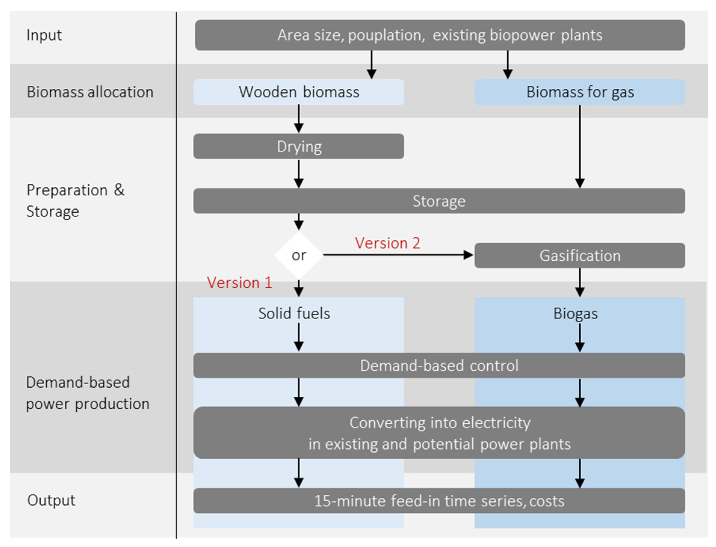
Figure 1 visualizes the methodology.
Obligatory input parameters include area size and population as well as existing biopower plants. If available, an individual load profile, agricultural land use shares and the local livestock can be inserted. If not available, these variables are statistically calculated based on standard allocation factors.
In a first model step, the biomass allocation is calculated. The available biomass is divided into wooden biomass and biomass for gasification. Relevant waste products from animal farming include liquid and solid manure from cattle, pigs and poultry. Other animal groups can be neglected as they represent less than 5% of the total livestock in Germany [21].
Relevant agricultural waste products in Germany include leaves from sugar beet, wooden biomass and green waste from forest or grounds maintenance, organic waste and private sector as well as municipal waste products (domestic, bulky and garden waste) [22]. Relevant energy crops include silage maize, sugar beet, oatlage, grain kernel, cup plant and grassland [23].
Energy crops are determined based on the available agricultural area. It is assumed that 14% of the agricultural area is used for energy crops, 62% of which are produced for biogas [23]. The biomass yield per crop is calculated based on standard allocation factors, listed in Table 3 [24].
Waste products from animal farming are calculated under consideration of standard allocation factors [25,26,27,28]. Wooden biomass and green waste from forest or grounds maintenance are approximated based on common land use shares in Germany [29]. For organic waste from industry and private sector as well as municipal waste products mean factors for distribution based on population and area size respectively are used [22]. The collected biomass is then combusted for power generation, either after transformation into biogas or as solid fuel.
In a second step, the energy yield of the available biomass mass flow is calculated under consideration of preparation & storage. For wooden biomass, this includes a drying process. For biomass for gas, the gasification process in included. If the available biomass exceeds the capacities of existing bioenergy plants, new plants are dimensioned. Depending on the kind of excess biomass (wooden biomass or biogas), CHP (combined heat and power plant) with either gas or steam turbine are chosen. Finally, the biopower feed-in depending on the local demand under consideration of available wind and solar power is calculated. Adding to the power output, the heat output is calculated, but neglected in this study.
The efficiency of the power plants depends on type and size as well as full load hours. In correlation with the current funding scheme in Germany, the economically most valuable variations are determined. For further details on the economic analysis at the example of an use case see [30].
To assess the degree of self-sufficiency, meaning the coverage share of local power demand with local supply, the feed-in and demand time series are compared. It is evaluated in how many time steps, the local feed-in covers or exceeds the local demand load (compare Section 3). It is to be emphasized, that in this study only timesteps with full coverage count as self-sufficient. This approach is chosen, because only with full coverage relying on the transmission grid becomes obsolete and economic advantageous can be gained through municipal energy supply. While when looking at annual net balances with disregard to time-series analysis, the dependence of the municipal grid on the overarching grid infrastructure is increasing instead of relieving the transmission grid [31]. Consequently, the potential of biomass is determined in a flexible control manner: bioenergy is only fed-in at times when wind and solar power cannot fully cover the local demand. To visualize this connection, see Figure 2. Biomass power is only provided at times when solar and wind power cannot fully cover the local demand. This way, storable biomass is on hold until needed to balance off-sets in power demand and supply. In this example, a further expansion of wind and solar power is definitely needed.
To ensure a certain reliability, validation of the model is provided by exemplary comparison of the results with the established potential model by [21]. The comparison for ten municipalities in both rural and urban Germany is shown in detail in Table 4.
In general, the validation results are satisfying, the deviation ranging between 30% over- and 19% underestimation. As the comparative study identifies different, strongly varying scenarios, the deviation to the BioPot results is considered acceptable.

2.2. Cluster Analysis

In the following, the data collection as well as the cluster analysis are described. The previously introduced methodology is then applied to the identified clusters to analyse the potential for self-sufficient energy systems. The cluster analysis provides a suitable tool to find patterns and correlations in large groups of data without time-intensive individual analyses. Hierarchically agglomerative cluster analysis with the Ward algorithm is chosen because it’s considered the best suited method for municipal cluster analyses [13,20]. The cluster analysis is conducted in RStudio.
Counties in rural Germany are clustered including 18 indicators consisting of publicly available data. Following an official definition, rural is characterised as counties with 845 or less inhabitants per square kilometre [32]. This includes 46.9 million people and 90% of the total area in Germany [
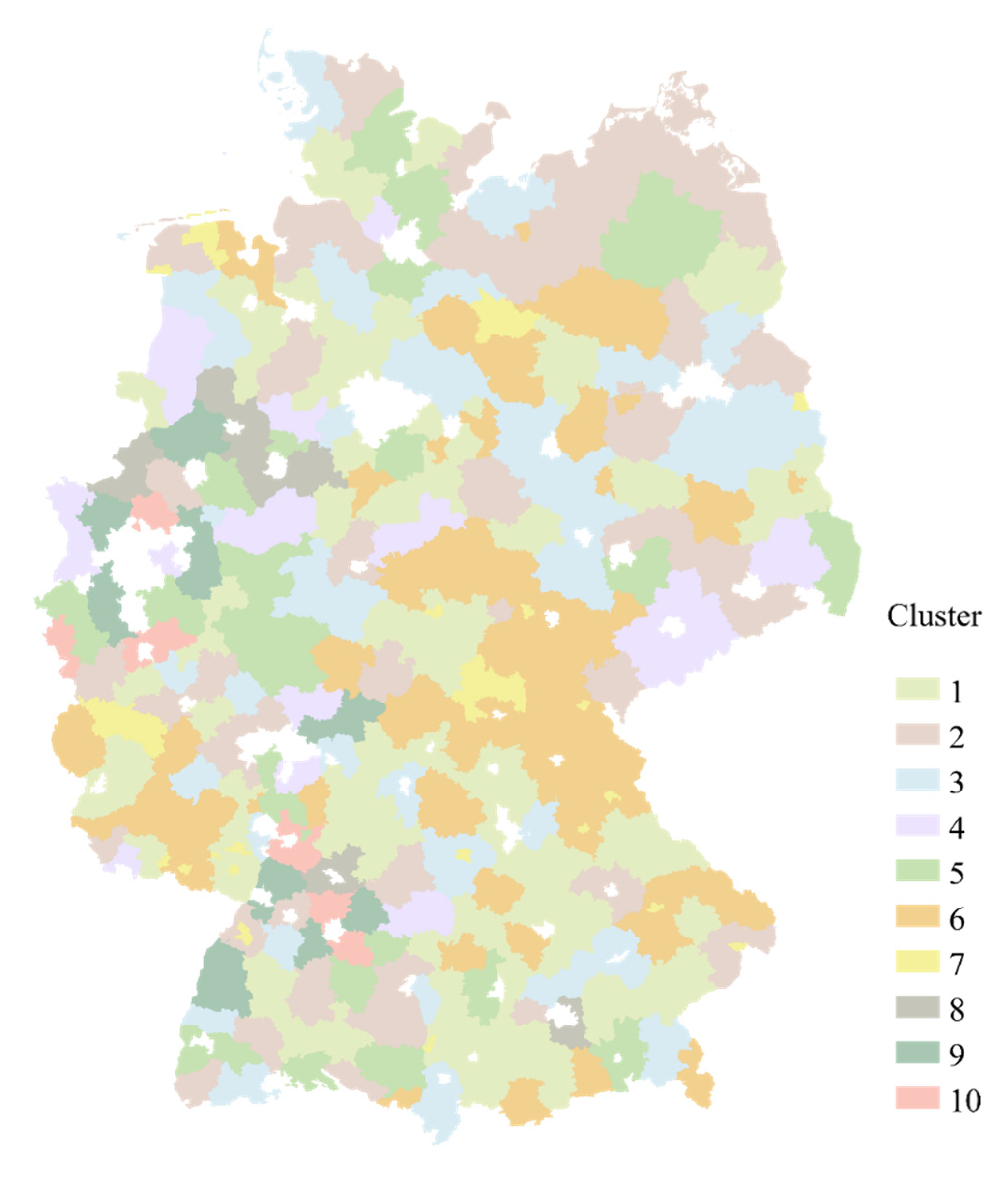
33]. The county level is chosen as trade-off between to data availability and area size. In total, 319 rural counties are clustered.
In hierarchically agglomerative cluster analyses the number of clusters is not known in advance. In this study, the number of ten clusters was determined without thorough analysis rather than educated guessing. This approach needs sophistication in further research.
Table 5 shows the most important cluster criteria.
18 indicators are claimed relevant in the context of municipal energy supply systems roughly divided into “Demand Load & liquidity” and “Potential & Acceptance”. The data is collected from different, publicly available sources and standardised according to [13]. All indicators are listed in Table 6. The reference years vary depending on data availability (see sources in Table 6).
“Demand Load & liquidity” includes data regarding the demand side of the energy system. Number of inhabitants as well as motor vehicles are influencing the demand load and demand load development, considering a growing electric vehicle branch. Unemployment rate and debt influence the potential liquidity of a county to implement further RES projects.
“Potential & Acceptance” on the other hand influences the techno-economical potential with regard to social interests. The area as well as the shares of certain land use types as settlement, traffic, agriculture and areas free of vegetation (waste land) leads to insights on available sights for new RES projects. Furthermore, the potential in biofuels, both waste products and energy crops, can be depicted. The already installed capacities of different energy sources, both renewables and fossil fuels, lead to the feed-in structure and the age group can give information on the potential acceptance of new RES projects [34,35,36].
Not all indicators are relevant in the context of this specific study. However, regarding a broader applicability of the method, the consideration of further indicators is reasonable.
Table 6. Indicators for cluster analysis.
Demand Load & LiquidityPotential & Acceptance
IndicatorUnitSourceIndicatorUnitSource
Inhabitants-[37]Areakm2[38]
Unemployment%[39]Settlement%[40]
Debt€/person[41]Traffic%[40]
Motor vehicles-/person[42]Agriculture%[40]
Free of vegetation%[40]
BioenergykW/km2[20]
GeothermalkW/km2[20]
Solar powerkW/km2[20]
Nuclear powerkW/km2[20]
StoragekW/km2[20]
Fossil energykW/km2[20]
Hydroelectric PowerkW/km2[20]
Wind powerkW/km2[20]
Age Group 16–66 yrs%[43]

3. Results and Discussion

In the following, the clustering results are presented. Then, the RES modelling is applied to the clusters and the results for demand as well as wind, solar and biomass feed-in are presented.
The cluster analysis results in ten different clusters. The spatial distribution of each cluster can be seen in Figure 3 and the respective mean values for each indicator are listed in Table 7.
Population and area size differ quite broadly. The other indicators are more evenly distributed except for water and geothermal power as well as storage capacities. Water and geothermal power are dependent on natural resources that are limited in regional dispersion. Storage capacities are not yet well established and therefore vary strongly among regions. Most clusters allocate counties all over the country, except for clusters 8, 9 and 10, that concentrate in South-Western Germany.
Cluster 1 unites the highest number of counties and is in no indicator remarkably high or low. The allocated counties are broadly spread all over Germany. Cluster 2 unites the largest counties in area size and the highest share of agricultural areas, possibly leading to a high potential in bioenergy. Cluster 3 is noticeable in geothermal capacities as well as areas free of vegetation, possibly leading to high RES potential due to available sites. Cluster 4 stands out with high biomass, geothermal and fossil energy as well as storage capacities. Cluster 5 is second lowest in wind power, comparatively high in storage capacities and otherwise average. In cluster 6 both the share of 16- to 66-year-olds and the storage capacities are lowest, while wind power and areas free of vegetation are highest. Cluster 7 is noticeable in several regards: having both lowest population and lowest area size as well as no geothermal power and almost no storage capacities, it’s the cluster with highest water power and among the highest biomass and wind power. Furthermore, the unemployment rates are highest, possibly leading to investment difficulties due to less cashflow through taxes. Clusters 8, 9 and 10 allocate the least counties and are less evenly distributed over the country. Cluster 8 and 9 are quite similar with the exceptions of biomass—maximum in cluster 8—and storage capacities—maximum in cluster 9. Cluster 10 combines the most maximal values in age, population, settlement, solar power and fossil energy. It is to be noted, though, that clusters 8, 9 and 10 allocate the least counties. Consequently, the variety within the clusters is not as broad as it is in larger clusters.
After Clustering, the potential analysis for flexibilization of the power sector through biomass is applied to the clusters as described in Section 2.1. All relevant variables are listed in Table 8. Looking at the load profiles, as expected the highest annual consumption is in cluster 10, followed by cluster 8 and 9. As described in Section 2.1, the influencing parameter for the load profile calculation is the population, where clusters 8, 9 and 10 have the highest values. The RES power production is a more complex value, generally depending on wind, solar and biomass power. As for wind and solar power, only the existing RES capacities are considered, consequently their feed-in directly depends on the cluster indicators “Solar Power” and “Wind Power”. Power production from biomass, however, is calculated in BioPot under consideration of both existing and in BioPot determined potential capacities.
While it was important to apply the installed capacity relative to the available area size in the clustering approach, in the following the total already installed capacity is listed in Table 8 for analysis.
In seven of the ten clusters, the potential capacity is higher than the installed capacity. This means, that there is still room for biomass extension in order to enhance the flexibilization of the power generation sector.
The potential biomass expansion ranges between a possible growth of 27% in cluster 1 towards the existing capacities to extensive potential of 92% in cluster 10. The highest potential is reached in clusters 2 (78%) and 10 (92%) and these two are among also the clusters with the least existing biomass capacities. By absolute numbers, cluster 2 hast the highest potential (52.55 MW), clearly a result of both the largest area size and the highest share of agricultural area. Considering the slim existing capacities in bioenergy, the need to tap the full potential in the counties of cluster 2 is clear.
Regarding the degree of self-sufficiency (time-integrated balance), the definition of self-sufficiency needs repetition: self-sufficiency is only reached at times when the local demand is fully covered or exceeded by local supply (compare Section 2.1). With biomass as flexible generation unit, offsets between supply and demand can be balanced. The self-sufficiency rates in Table 8 for all clusters range between 0% in cluster 10 and 12% in clusters 3 and 6. Clusters 4, 5 and 7 to 10 range very low up to 5%.
The average full load hours (FLH) of the bioenergy plants is another indicator for the degree of self-sufficiency: the less full-load hours, the less frequent the demand for bioenergy to balance load peaks. Accordingly, clusters 1–3 and 6 have the least FLH.

4. Discussion

In clusters 4, 7 and 8, BioPot does not identify further potential. One possible reason may be the already existing strong bioenergy infrastructure coming top 3 among all 10 clusters in relation to area size. Since area size is one of the main influencing variables in BioPot, this can explain the discrepancy. Consequently, the rather conservative potential estimation in BioPot needs to be considered in analysis. For those counties, allocated in a cluster with little or no expansion potential, a merging of clusters might be an option. This way, slight regional differences in supply and demand can be balanced without exceeding reliance on the overarching grid infrastructure. The advantage of local power supply can still be exploited and the regional energy system strengthened.
The highest potential is reached in clusters 2 (78%) and 10 (92%) and these two are among also the clusters with the least existing biomass capacities. Accordingly, the gap between reality and potential is highest and there is an urgent need for expansion.
The remarkably low self-sufficiency rate in clusters 4, 5, 7 and 10 can be explained by the population size. Except for cluster 7, these clusters have the largest populations. The demand load correlates positively with the population size and the higher the load the more challenging to cover it. Furthermore, the minima in wind power are among these clusters and clusters 5, 6, 9 and 10 show little biomass potential. Especially noticeable is 0% self-sufficiency in cluster 10 as this means that the local demand is covered by local supply less than 87.5 h of the year. Those clusters performing slightly better at self-sufficiency, have smaller population sizes, hence smaller demand loads to cover.
The FLH are another indicator for degree of self-sufficiency. Plants with little FLH can use their full capacities at times, when wind and solar power are low or when power demand is high. This concentrates the available biomass on balancing offsets more than providing base load.
Generally, all clusters need more generation capacities. Another option to shift load peaks might be storage integration or demand-side-management. However, the expansion of solar and wind power remains a crucial element. This becomes clear, when looking at the annual supply-demand-balance: those clusters with better degrees of self-sufficiency, also have higher annual supply-demand-balance. Consequently, only a strong over-dimensioning of the RES supply system can lead to self-sufficiency, where surplus energy can be stored or converted. This way, the supply-demand-offset at times with little sun and wind, can be balanced by bioenergy more easily. Currently, existing solar and wind power capacities leave too big a gap for bioenergy to cover.
Obviously, all clusters represent mean values. Hence, those counties with already existing strong over-dimensioning of wind and solar power are averaged out. For the individual identification of possible expansion projects, a thorough local analysis under participation of local stakeholders is necessary. However, this clustering approach can help identifying structural similarities and differences and drawing the bigger picture for a national strategy.

5. Conclusions and Outlook

The goal of the study was investigating what structural characteristics of counties are advantageous for self-sufficient power systems based on RES. A crucial element in this investigation is bioenergy as flexible generation unit. The methodology BioPot is introduced for bioenergy potential analysis under consideration of the local land use shares and demand loads. Both energy crops and waster products are considered. Adding to the power output, the heat output is calculated, but neglected in this study. BioPot is exemplarily validated for ten municipalities in rural and urban Germany. The model results are satisfying.
The bioenergy feed-in is adjusted considering the local demand under consideration of fluctuating solar and wind power feed-in. This way, biomass acts as flexible power unit, balancing offsets between power demand and supply. Wind and solar power are only roughly downscaled form national time series. The modelling of the power sector is coupled with a cluster analysis in order to draw a large-scale conclusion on structural characteristics beneficial or obstructive for municipal energy systems. Ten clusters were identified with the Ward algorithm in a hierarchical-agglomerative method. 319 rural counties in Germany were clustered with 18 indicators. The county level was chosen as a solid trade-off between regional agglomeration and data availability. Discussed output variables included solar, wind and biomass feed-in as well as self-sufficiency of the system. Furthermore, full load hours of bioenergy capacities are discussed.
Generally, a clustering approach is found suitable for energy system analysis. The clusters vary in their characteristics and show clear distinction. When applied to the energy system model, the results underline a further need for RES expansion projects in order to close the gap between supply and demand, especially at times with little wind and sun. Only then, bioenergy can effectively balance the offset and support a truly self-sufficient local energy system. While the model results indicate that the vast majority of the counties are suitable for further expansion and self-sufficiency, especially in cluster 10, this suitability is to be questioned. High population density always is a critical characteristic, because with it come both a high demand due to the large population and limited area size for further RES expansion projects.
Limitations of the study include the rough estimation of solar and wind power feed-in, only depending on installed capacity. The feed-in pattern is for all clusters the same, only varying in scale. The same applies to the standard load profiles. Both need further individualization taking into account different demand structures and local variations in wind and solar supply.
In future studies a validation of the clustering analysis by looking more closely at the individual counties within the clusters can be useful. Furthermore, the method for cluster determination needs sophistication. In the long-term, an integration of storage capacities and demand-side-management is important, to increase the potential in offset-balancing. Additionally, the integration of a European perspective might be considered. With the national grids in Europe being closely linked to each other, the effects of self-sufficient counties on the European power system needs to be considered. The exchange of experiences in designing and building self-sufficient systems can help making the whole System in Europe or even world-wide more renewable and resilient.

Author Contributions

Conceptualization, L.S.; methodology, L.S.; software, L.S., L.P. and T.S.; validation, L.S. and T.S.; writing—original draft preparation, L.S.; writing—review and editing, R.S.; visualization, L.S.; supervision, R.S. and G.J.; project administration, L.S.; funding acquisition, L.S. and R.S. All authors have read and agreed to the published version of the manuscript.

Funding

This research was funded by the German Federal Ministry for Economic Affairs and Energy, grant number 03ET4070A. The APC was also funded by the German Federal Ministry for Economic Affairs and Energy.

Institutional Review Board Statement

Not applicable.

Informed Consent Statement

Not applicable.

Data Availability Statement

The data used for this study is publicly available under [20,21,23,24,37,38,39,40,41,42,43,44].

Acknowledgments

We thank the Federal Ministry for Economic Affairs and Energy for funding the research project (acronym: ArkESE) in which we address this topic. In the three-year project (start December 2018), rural municipalities are investigated to design individual electricity supply systems based on renewables. Municipalities shall be enabled to prepare, make and implement energy system related decisions more self-sufficiently. The funding source had no particular involvement in this study.

Conflicts of Interest

The authors declare no conflict of interest. The funders had no role in the design of the study; in the collection, analyses, or interpretation of data; in the writing of the manuscript, or in the decision to publish the results.

References

  1. United Nations. The Paris Agreement. Available online: https://unfccc.int/process-and-meetings/the-paris-agreement/the-paris-agreement (accessed on 12 July 2021).
  2. Bundesministerium für Umwelt, Naturschutz und Nukleare Sicherheit (BMU). Lesefassung des Bundes-Klimaschutzgesetzes 2021: KSG; Bundesministerium für Umwelt, Naturschutz und nukleare Sicherheit (BMU): Berlin, Germany, 2021. [Google Scholar]
  3. Jenssen, T.; König, A.; Eltrop, L. Bioenergy villages in Germany: Bringing a low carbon energy supply for rural areas into practice. Renew. Energy 2012, 74–80. [Google Scholar] [CrossRef]
  4. Schreiber, M. Bewertungskriterien einer optimierten Energieversorgung regionaler Verbünde mit hohen Anteilen erneuerbarer Erzeugung. Z. Energ. 2012, 36, 257–265. [Google Scholar] [CrossRef]
  5. Verband deutscher Ingenieure. Energiespeicher; VDI-Statusreport: Düsseldorf, Germany, 2017. [Google Scholar]
  6. Tafarte, P.; Hennig, C.; Dotzauer, M.; Thrän, D. Impact of flexible bioenergy provision on residual load fluctuation: A case study for the TransnetBW transmission system in 2022. Energy Sustain. Soc. 2017, 7, 3. [Google Scholar] [CrossRef] [Green Version]
  7. Thrän, D.; Dotzauer, M.; Lenz, V.; Liebetrau, J.; Ortwein, A. Flexible bioenergy supply for balancing fluctuating renewables in the heat and power sector—a review of technologies and concepts. Energy Sustain. Soc. 2015, 5, 35. [Google Scholar] [CrossRef] [Green Version]
  8. Schmidt, J.; Schönhart, M.; Biberacher, M.; Guggenberger, T.; Hausl, S.; Kalt, G.; Leduc, S.; Schardinger, I.; Schmid, E. Regional energy autarky: Potentials, costs and consequences for an Austrian region. Energy Policy 2012, 47, 211–221. [Google Scholar] [CrossRef]
  9. Peter, S. Modellierung einer vollständig auf erneuerbaren Energien basierenden Stromerzeugung im Jahr 2050 in autarken, dezentralen Strukturen. Studie im Auftrag des Umweltbundesamtes (UBA). Clim. Chang. 2013. Available online: https://www.umweltbundesamt.de/sites/default/files/medien/376/publikationen/climate_change_14_2013_modellierung_einer_vollstaendig_auf_erneuerbaren_energien.pdf (accessed on 23 August 2021).
  10. Hahn, H.; Krautkremer, B.; Hartmann, K.; Wachendorf, M. Review of concepts for a demand-driven biogas supply for flexible power generation. Renew. Sustain. Energy Rev. 2014, 29, 383–393. [Google Scholar] [CrossRef]
  11. Hansen, K.; Breyer, C.; Lund, H. Status and perspectives on 100% renewable energy systems. Energy 2019, 175, 471–480. [Google Scholar] [CrossRef]
  12. Funcke, S.; Bauknecht, D. Typology of centralised and decentralised visions for electricity infrastructure. Util. Policy 2016, 40, 67–74. [Google Scholar] [CrossRef]
  13. Weinand, J.; McKenna, R.; Fichtner, W. Developing a municipality typology for modelling decentralised energy systems. Util. Policy 2018, 57, 75–96. [Google Scholar] [CrossRef] [Green Version]
  14. Bundesverband der Energie- und Wasserwirtschaft. Standardlastprofile Strom. Available online: https://www.bdew.de/energie/standardlastprofile-strom/ (accessed on 4 September 2019).
  15. Fraunhofer ISE. Energy Charts. Available online: https://www.energy-charts.de/index_de.htm (accessed on 4 September 2019).
  16. Destatis. Stromverbrauch der Privaten Haushalte nach Haushaltsgrößenklassen: Umweltökonomische Gesamtrechnung. Available online: https://www.destatis.de/DE/Themen/Gesellschaft-Umwelt/Umwelt/UGR/private-haushalte/Tabellen/stromverbrauch-haushalte.html (accessed on 5 January 2021).
  17. Neiber, J. Energieeffizienz in der Landwirtschaft: Von der Theorie zur Praxis—Energieverbrauchsmessungen an Landwirtschaftlichen Betrieben. 30 January 2014. Available online: https://docplayer.org/11225956-Energieeffizienz-in-der-landwirtschaft-von-der-theorie-zur-praxis-energieverbrauchsmessungen-an-landwirtschaftlichen-betrieben.html (accessed on 23 August 2021).
  18. Fachhochschule Münster. Kommunalsteckbrief Steinfurt. 2012. Available online: https://formular-server.de/KAAW_FS/findform?shortname=kstst_0000000000003&formtecid=2&areashortname=Kreisstadt_Steinfurt (accessed on 23 July 2021).
  19. Bundesministerium für Wirtschaft und Energie. Zeitreihen zur Entwicklung der Erneuerbaren Energien in Deutschland: Unter Verwendung von Daten der Arbeitsgruppe Erneuerbare Energien-Statistik (AGEE-Stat). 2021. Available online: https://www.erneuerbare-energien.de/EE/Redaktion/DE/Downloads/zeitreihen-zur-entwicklung-der-erneuerbaren-energien-in-deutschland-1990-2020.pdf;jsessionid=740655FF84BA0E296EB106739699550C?__blob=publicationFile&v=31 (accessed on 21 July 2021).
  20. Bundesnetzagentur. Marktstammdatenregister. Available online: https://www.marktstammdatenregister.de/MaStR (accessed on 17 July 2021).
  21. Landesamt für Natur; Umwelt und Verbraucherschutz NRW. LANUV-Fachbericht 40—Teil 3 Biomasse-Energie; Landesamt für Natur, Umwelt und Verbraucherschutz Nordrhein-Westfalen: Recklinghausen, Germany, 2014. [Google Scholar]
  22. Kaltschmitt, M.; Hartmann, H.; Hofbauer, H. Energie aus Biomasse: Grundlagen, Techniken und Verfahren, 3rd ed.; Springer: Berlin/Heidelberg, Germany, 2016; ISBN 9783662474372. [Google Scholar]
  23. Fachagentur Nachwachsende Rohstoffe, e.V. Anbauzahlen: Energiepflanzenanbau für Biogas. 2020. Available online: https://pflanzen.fnr.de/anbauzahlen (accessed on 15 July 2021).
  24. Fachagentur Nachwachsende Rohstoffe, e.V. Pflanzen. Available online: https://pflanzen.fnr.de/energiepflanzen/pflanzen (accessed on 15 July 2021).
  25. Deutscher Bundestag. Kurzinformation: Raumgewicht und Rauminhalt von Wirtschaftsdüngerarten; Fachbereich WD 8 (Umwelt, Naturschutz, Reaktorsicherheit, Bildung und Forschung): Berlin, Germany, 2017. [Google Scholar]
  26. Kuratorium für Technik und Bauwesen in der Landwirtschaft. Wirtschaftlichkeitsrechner Biogas. Available online: https://www.ktbl.de//webanwendungen/wirtschaftlichkeitsrechner-biogas/ (accessed on 4 September 2019).
  27. Statistisches Bundesamt. Land und Forstwirtschaft, Fischerei: Viehbestand; Statistisches Bundesamt: Wiesbaden, Germany, 2018. [Google Scholar]
  28. Statistisches Bundesamt. Land- und Forstwirtschaft, Fischerei: Tiere und Tierische Erzeugung. Available online: https://www.destatis.de/DE/Themen/Branchen-Unternehmen/Landwirtschaft-Forstwirtschaft-Fischerei/Tiere-Tierische-Erzeugung/_inhalt.html (accessed on 4 September 2019).
  29. Statistisches Bundesamt. Land- und Forstwirtschaft, Fischerei: Bodenfläche Nach Art der Tatsächlichen Nutzung; Statistisches Bundesamt: Wiesbaden, Germany, 2018. [Google Scholar]
  30. Blickwedel, L.; Stößel, L.; Schelenz, R.; Jacobs, G. Multicriterial Evaluation of Renewable Energy Expansion Projects at Municipal Level for the Available Biomass Potential. Energies 2020, 13, 6211. [Google Scholar] [CrossRef]
  31. McKenna, R. The double-edged sword of decentralized energy autonomy. Energy Policy 2018, 113, 747–750. [Google Scholar] [CrossRef]
  32. Bundesministerium für Ernährung und Landwirtschaft. Infoportal Zukunft.Land. Available online: https://www.landatlas.de/laendlich/bevdichte.html (accessed on 16 August 2019).
  33. Bundesministerium für Ernährung und Landwirtschaft. Ländliche Regionen Entdecken. Available online: https://www.bmel.de/DE/Laendliche-Raeume/Infografiken/_node.html (accessed on 23 August 2021).
  34. Bertsch, V.; Hall, M.; Weinhardt, C.; Fichtner, W. Public acceptance and preferences related to renewable energy and grid expansion policy: Empirical insights for Germany. Energy 2016, 114, 465–477. [Google Scholar] [CrossRef]
  35. Hobman, E.V.; Ashworth, P. Public support for energy sources and related technologies: The impact of simple information provision. Energy Policy 2013, 63, 862–869. [Google Scholar] [CrossRef]
  36. Musall, F.D.; Kuik, O. Local acceptance of renewable energy—A case study from southeast Germany. Energy Policy 2011, 39, 3252–3260. [Google Scholar] [CrossRef]
  37. Statistische Ämter des Bundes und der Länder. Bevölkerung nach Geschlecht: Regionale Tiefe: Kreise und Kreisfreie Städte. Available online: https://www.regionalstatistik.de/genesis//online?operation=table&code=12411-01-01-4&bypass=true&levelindex=0&levelid=1626533105747#abreadcrumb (accessed on 19 July 2021).
  38. Statistische Ämter des Bundes und der Länder. Gebietsfläche in qkm—Stichtag 31.12.: Regionale Tiefe: Kreise und krfr. Städte. Available online: https://www.regionalstatistik.de/genesis//online?operation=table&code=11111-01-01-4&bypass=true&levelindex=0&levelid=1626532168016#abreadcrumb (accessed on 19 July 2021).
  39. Statistische Ämter des Bundes und der Länder. Arbeitslose Nach Ausgewählten Personengruppen—Jahresdurchschnitt: Regionale Tiefe: Kreise und krfr. Städte. Available online: https://www.regionalstatistik.de/genesis//online?operation=table&code=13211-01-03-4&bypass=true&levelindex=0&levelid=1626539297854#abreadcrumb (accessed on 23 August 2021).
  40. Statistische Ämter des Bundes und der Länder. Bodenflächen nach Art der Tatsächlichen Nutzung—Stichtag 31.12: Regionale Tiefe: Kreise und kreisfreie Städte. Available online: https://www.regionalstatistik.de/genesis//online?operation=table&code=33111-01-02-4&bypass=true&levelindex=0&levelid=1626531275512#abreadcrumb (accessed on 19 July 2021).
  41. Statistische Ämter des Bundes und der Länder. Schulden (bis 2009): Regionale Tiefe: Kreise und krfr. Städte. Available online: https://www.regionalstatistik.de/genesis/online?operation=previous&levelindex=1&step=1&titel=Tabellenaufbau&levelid=1626535015006&acceptscookies=false#abreadcrumb (accessed on 19 July 2021).
  42. Statistische Ämter des Bundes und der Länder. Kraftfahrzeugbestand nach Kraftfahrzeugarten—Stichtag 01.01.: Regionale Tiefe: Kreise und krfr. Städt. Available online: https://www.regionalstatistik.de/genesis/online#astructure (accessed on 19 July 2021).
  43. Statistisches Bundesamt. Interaktive Karte Mit Altersgruppen auf Kreisebene 2019: Bevölkerung 16 bis unter 60 Jahre. Available online: https://www.destatis.de/DE/Themen/Gesellschaft-Umwelt/Bevoelkerung/Bevoelkerungsstand/karte-altersgruppen.html (accessed on 20 April 2021).
  44. Statistisches Bundesamt. Bevölkerungsdichte (Einwohner je km2) in Deutschland von 1991 bis 2017. Available online: https://de.statista.com/statistik/daten/studie/440766/umfrage/bevoelkerungsdichte-in-deutschland/ (accessed on 16 August 2019).
Figure 1. BioPot methodology.
Energies 14 05227 g001
Figure 2. Exemplary week of RES feed-in in an exemplary county. Biomass power is only provided at times when wind and solar power cannot fully cover the local demand.
Energies 14 05227 g002
Figure 3. Spatial distribution of identified clusters.
Energies 14 05227 g003
Table 1. Variables included in the analysis. All variables are time series in 15-min resolution for one exemplary year (2018) in MW.
Variable TypeBase Source
Load ProfileStandard Load profiles [14]
Photovoltaic feed-inFraunhofer Energy Charts [15]
Wind power feed-inFraunhofer Energy Charts [15]
Bioenergy feed-inBioPot
Table 2. Exemplary valdiation of load profile calculation.
County [18]Model
Households [MWh/a]51,39953,157
Industry [MWh/a]82,531142,710
Agriculture [MWh/a]38533860
Table 3. Applied allocation factors for biomass resources.
Energy Crop Type [23,24]%Yield (Tons Fresh Matter/ha)
Silage maize6466.44
Sugar beet175
Oatlage740.2
Grain kernel136.5
Cup plant155.6
Grassland1424.3
Table 4. Validation for bioenergy potential assessment in BioPot. Reference results provided by [21].
MunicipalityResults BioPot (GWh/a)Deviation
Borken344−14%
Coesfeld261+19%
Düren278−5%
Euskirchen289+13%
Gütersloh248+24%
Hagen55+17%
Köln222−19%
Leverkusen37−16%
Münster98+21%
Paderborn300+30%
Table 5. Cluster criteria.
ObjectsCounties in Rural Germany
Indicators18
AlgorithmWard
Cluster Analysis MethodHierarchical-agglomerative
Number of clusters10
Software usedRStudio
Table 7. Characteristics of identified clusters.
ClusterUnitC 1C 2C 3C 4C 5C 6C 7C 8C 9C 10
N° of counties-774339172869236116
Inhabitants-129,312211,388170,526313,370265,99189,85349,879356,133432,029566,788
Age Group 16–66 years%55.654.855.455.055.854.054.857.156.357.2
Unemployment rate%2.02.22.32.62.42.52.82.02.52.7
Debt€/person77.790.694.478.692.2104.9122.473.790.298.2
Motor vehicles-/person0.80.80.80.80.80.60.80.60.90.8
Areakm21000.41493.71316.71306.41291.7878.9279.81253.71048.4835.2
Settlement%8.18.88.612.511.18.615.512.515.818.1
Traffic%4.95.04.95.95.74.97.05.96.77.9
Agriculture%49.353.851.951.849.647.140.453.545.942.5
Free of vegetation%1.10.81.40.70.61.71.40.80.60.6
BioenergykW/km224.319.827.735.719.022.432.337.921.017.5
GeothermalkW/km20.30.12.47.40.00.20.07.17.64.0
Solar powerkW/km2151.3145.2125.8138.1138.4113.5192.0220.0244.6392.4
Nuclear powerkW/km261.40.026.827.30.00.00.0198.50.00.0
StoragekW/km24.45.63.19.06.62.12.74.311.47.8
Fossil energykW/km2125.036.2134.9301.990.7173.0134.9132.9241.8398.9
Hydroelectric PowerkW/km214.57.67.23.08.612.847.95.83.38.5
Wind powerkW/km2173.9174.5190.6173.2118.4205.6190.7190.5159.0112.0
Table 8. RES modelling results for each cluster.
UnitC 1C 2C 3C 4C 5
Load profileMWh981,8501,556,9001,295,6001,973,7001,740,700
RESMWh492,141728,583662,909625,457473,843
Annual balance%5047513227
Time-integrated balance%9101242
PVMWh135,698.82194,339.30148,509.34161,693.66160,236.88
WindMWh356,252.60533,913.81514,121.72463,465.61313,329.91
Biomass (BM)
BM installed capacityMW24.3129.5436.4946.6624.54
BM potential capacityMW6.5323.0010.57012.45
BM potential growth%27%78%29%0%51%
BM net power productionMWh190.31330.23278.76297.80276.40
BM full load hoursh/a6670.446792.376402.857837.548075.23
UnitC 6C 7C 8C 9C 10
Load profileMWh748,210338,8002,159,7002,442,5003,007,100
RESMWh459,618157,468736,634571,405485,580
Annual balance%6146342316
Time-integrated balance%125310
PVMWh89,408.3748,154.44247,180.39229,825.64293,780.61
WindMWh370,051.90109,269.63489,152.84341,336.91191,584.91
Biomass (BM)
BM installed capacityMW19.679.0347.5322.0514.63
BM potential capacityMW10.76009.7513.41
BM potential growth%55%0%0%44%92%
BM net power productionMWh158.1744.41300.82242.63215.45
BM full load hoursh/a5618.267185.067852.868245.768300.75
Publisher’s Note: MDPI stays neutral with regard to jurisdictional claims in published maps and institutional affiliations.

