1. Introduction
Geotechnical Seismic Isolation (GSI) consists of a novel technique that applies different materials to reduce costs (installation and maintenance of the devices) connected with traditional base isolation. In this regard, many materials have been proposed, such as rubber–soil mixtures (RSM), geofoam, geomembranes/geotextiles, rocking isolation and natural stone pebbles, and kart tyres, as shown in [
1]. In particular, extensive research was conducted on polyurethane, injectable in the soil below structures (new and existing ones), as shown in [
2,
3,
4]. Other researchers proposed the use of sand and sand–bitumen mixtures [
5,
6,
7] as GSI isolation materials.
On one side, GSI is conceivably an environmentally friendly and low-cost technology particularly valid for developing countries. On the other side, due to the level of its novelty, GSI applications required many experiments to prove their reliability. In this regard, experimental tests were conducted on shaking tables [
8,
9]. Tsiavos et al. [
10] performed direct shear tests and small-scale 1 g shaking table tests. Tsang et al. [
11] conducted centrifuge tests, while Kaneko et al. [
12] proposed hybrid simulations. Another typology of verifications consists of numerical simulations, such as in [
13,
14,
15,
16,
17]. In particular, the authors of [
13] investigated the application of granulated rubber–soil mixtures to the seismic isolation for low-to-medium-rise buildings. Nonlinear models were proposed in [
14] to study seismic isolation systems made of recycled tire-rubber. The application of GSI on bridges configurations was also proposed, [
18].
It was recently demonstrated [
1] that GSI effectiveness depends on the dynamic characteristics of the input motion in relation to the properties of the structure (mainly the fundamental periods). In order to extend the previous outcomes with numerical simulations, the present paper assesses GSI with a probabilistic-based approach based on developing analytical fragility curves in order to consider all the uncertainties connected with the definition of input motions. In particular, this paper aims to extend the previous contributions by considering several structural configurations with different parameters (in terms of stiffness and mass) to consider the effectiveness of GSI for realistic buildings. Therefore, it is possible to consider the following novelties:
Simulating different structural configurations with different location of the liner (0.5 m, 10 m, 20 m and 30 m depth) to aid better insight into the role of GSI on different buildings.
Proposing parametric studies on several structural parameters (mass, stiffness) in order to relate the efficiency of GSI with the structural behaviours.
Development of analytical fragility curves that may consider the uncertainties with a probabilistic-based approach.
The paper is organized into six sections. In
Section 2, the numerical models are presented and discussed.
Section 3 clarifies the choice of the earthquakes applied in the study, while
Section 4 shows the characteristics of the soils. Results are shown and discussed in
Section 5, followed by the conclusions.
2. Numerical Model
Numerical simulations were performed with OpenSeesPL (an open-source computational platform) [
18], by the Pacific Earthquake Engineering Research (PEER) centre. In particular, the Opensees PL platform, developed by the authors of [
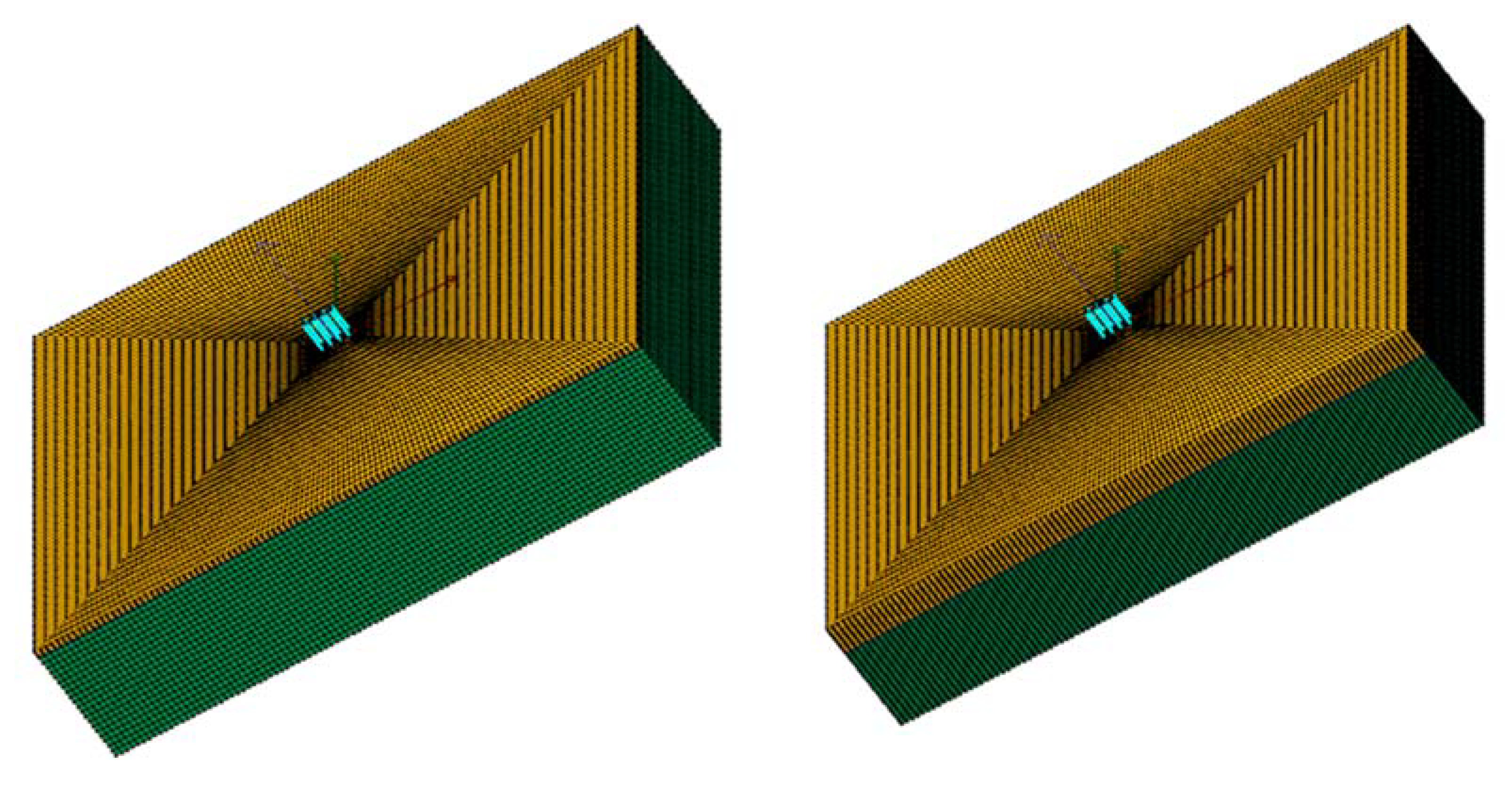
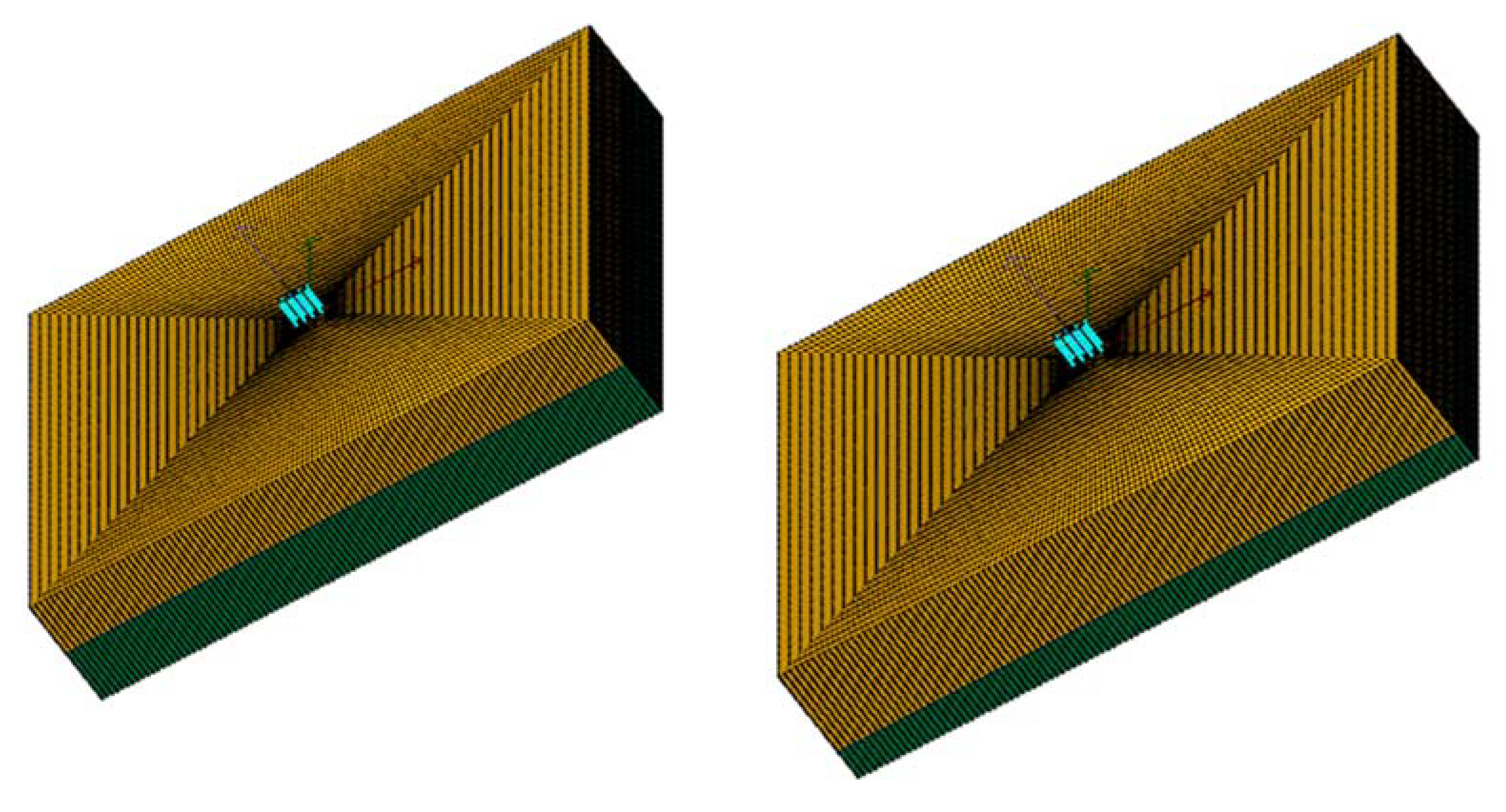
19] at University of California, San Diego, was applied to model the different case studies. Tridimensional soil meshes were described with BrickUP isoparametric elements. These elements allow to consider both the displacements (longitudinal, transversal and vertical: degree of freedom: 1, 2 and 3, respectively) to simulate the dynamic response of the soil. One 3D mesh for every considered configuration (total: 4, as shown in
Figure 1) has been implemented to model a building resting on a sandy soil domain. What changes between the 4 3D meshes is the location of GSI that is located between the first (yellow) layer and the second (green) layer that have the same the same properties. The dimensions of the elements inside the mesh followed the previous contributions [
1,
17]. Furthermore, the performance of the lateral boundaries was verified by comparing the accelerations at the top of the mesh with those obtained under the free field (FF) conditions to reproduce wave mechanisms. Mesh discretization was derived considering a 100 m/s as the lowest shear wave velocity and a 10 Hz as the maximum frequency.
Soil structure interaction has the main contribution in defining the effects of the soil on the structure and was herein modelled with several assumptions: (1) Particular attention has been paid to the boundary conditions, where absorbing boundaries have been applied at the base to dissipate the radiating waves. (2) The base nodes have been set free to move along the longitudinal and transversal directions to model the elastic half-space below the mesh, while vertical direction was fixed. (3) The lateral nodes have been constrained to simulate pure shear by applying period boundaries and to ensure free field conditions (that are not disturbed by the presence of the structure). At the lateral nodes, a penalty method (tolerance = 10
−4) has been adopted to avoid problems with equations system conditions [
18]. (4) The connections between the shallow foundations and the soil were built up as equal and can impose the displacements to be the same between the structure and the soil nodes and thus to capture the rocking component of the SSI. (5) The soil deposit was simulated using the multi-surface plasticity constitutive model [
19]. Note that the presence of shallow foundations allows to consider kinematic interaction as the main source of SSI between the soil and the structure, as demonstrated in [
20,
21].
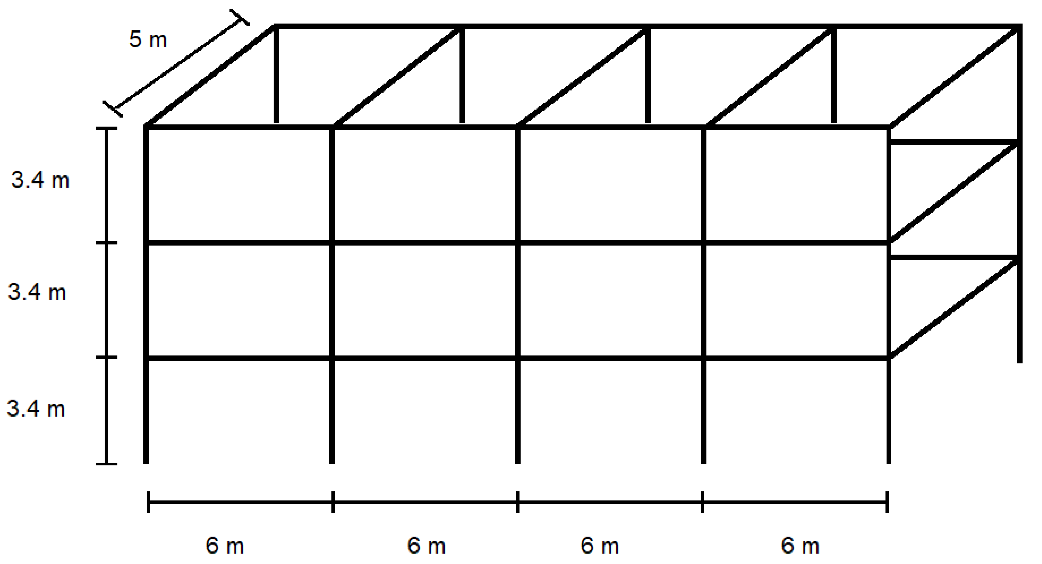
The benchmark reinforced concrete structure (
Figure 2) was calibrated to be representative of residential low-rise building, performing the structure considered in [
1] and called S1, with three floors (3.4 m each). Four columns in longitudinal direction (6 m spaced) and 2 in transversal direction (5 m spaced). The columns and the beams have been modelled with elastic beam column elements using the properties shown in
Table 1.
Shallow foundation was considered (slab dimensions: 28.4 m × 34.4 m, thickness: 0.5 m) and a rigid concrete slab was modelled by applying equal degree of freedom to connect the nodes at the base of the columns with those of the soil domain. In order to simulate the interface between the columns and the slab, horizontal rigid links were defined, following the works in [
1,
17]. The foundation slab has been modelled elastically with an equivalent material that simulates the concrete and implementing the pressure independent multi-yield model (PIMY) [
19], with the properties as shown in
Table 2. The design of the foundation consisted in assessing the eccentricity for the most severe condition: minimum vertical loads (gravity and seismic loads) and maximum bending moments.
Both GSI and the soil were modelled with a nonlinear hysteretic material named Pressure-Independent Multiyield [
19] that applies a Von Mises multi-surface kinematic plasticity approach and an associate flow rule to capture both monotonic and hysteretic elasto-plastic response of both the soil and GSI. According to this formulation, plasticity is exhibited only in the deviatoric stress–strain response, while volumetric response is linear-elastic. Several GSI configurations were considered, by following the contributions proposed by [
15] GSI1, GSI2, GSI3 and GSI4, with different position of the liner: at foundation level, at 10 m, 20 m and 30 m depth, respectively.
Table 3 shows the number of elements and nodes used for the 3D numerical model. GSI was modelled in order to represent realistically a thin layer of deformable material, following the calibration proposed in [
15], whose parameters are shown in
Table 4. Some of these parameters (such as the density, Poisson’s ratio) have little effect on the performance of GSI and were widely investigated by the authors of [
13]. The soil was considered stiff, as it was demonstrated in [
15] that the effectiveness of GSI depends on soil deformability. In particular, such conditions represent the case of a hard soil or a ground that has been strengthened with several techniques, such as densification. The parameters of the soil have been adopted from the one called Soil A in [
15] and shown in
Table 4.
3. Nonlinear Analyses
Seventy earthquake records from the PEER NGA database (
http://peer.berkeley.edu/nga/, accessed on 18 August 2021) were employed in the analyses to study the effect of the earthquake intensity on the response of the buildings. They were chosen in order to represent several intensities and reproduce soil deformations (and thus soil structure interaction) for several historical earthquakes. In particular,
Table 5 presents the name, station, duration and peak ground acceleration (PGA) for each record.
The nonlinear dynamic analyses were performed by following the approach adopted in [
20,
21] which consists of running three steps (stages): In the first step, the soil initial stresses were calculated considering linear properties (weight, shear and bulk modulus). In step 2, the structure and the associated loads were applied, and the properties of the soil were changed from elastic to plastic. Twenty-five load steps were necessary in order to maintain the convergency requirements. Finally, Step 4 consisted of applying the input motion at the base of the soil mesh as acceleration time history. NewtonLineSearch algorithm was used in the analyses of Step 4.
4. Fragility Curves
This paper develops analytical fragility curves on the bases of the analyses that were performed with the 4 configurations and 70 input motions (total: 280 analyses). Fragility curves were proposed in the past decades for RC buildings (as shown in [
21]) as graphical representations of the between the probability of exceeding selected damage states (DS) for levels of engineering demand parameters (EDP). They are useful for the assessments of damages at different levels of Intensity Measures (IM). In this paper, several assumptions were considered: (1) PGA is considered as the reference Intensity measure, (2) inter-story drift was considered as the reference EDP, (3) four states (slight, moderate, extensive and complete) were defined for interstory drifts 0.33%, 0.58%, 1.56% and 4%, respectively, as proposed in [
22]. In addition, (4) all uncertainties are represented by lognormal distributions. This allows to consider two representative parameters: the lognormal standard deviation (β) and the mean (μ) of the lognormal seismic intensity measure, as detailed in [
21].
Therefore, the results from the performed nonlinear analyses were used to build linear regressions and define the median and log-standard deviation values. The probability of exceedance for a specific PGA value was then calculated as
where,
P is the probability of the structural damage (D) exceeding the i-th damage state (C);
Φ is the standard normal cumulative distribution function;
PGA (Peak Ground Acceleration) is the selected intensity measure value;
β is the lognormal standard deviation and
µ is the mean value of the lognormal seismic intensity measure (PGA).
5. Results
Following the previous contribution [
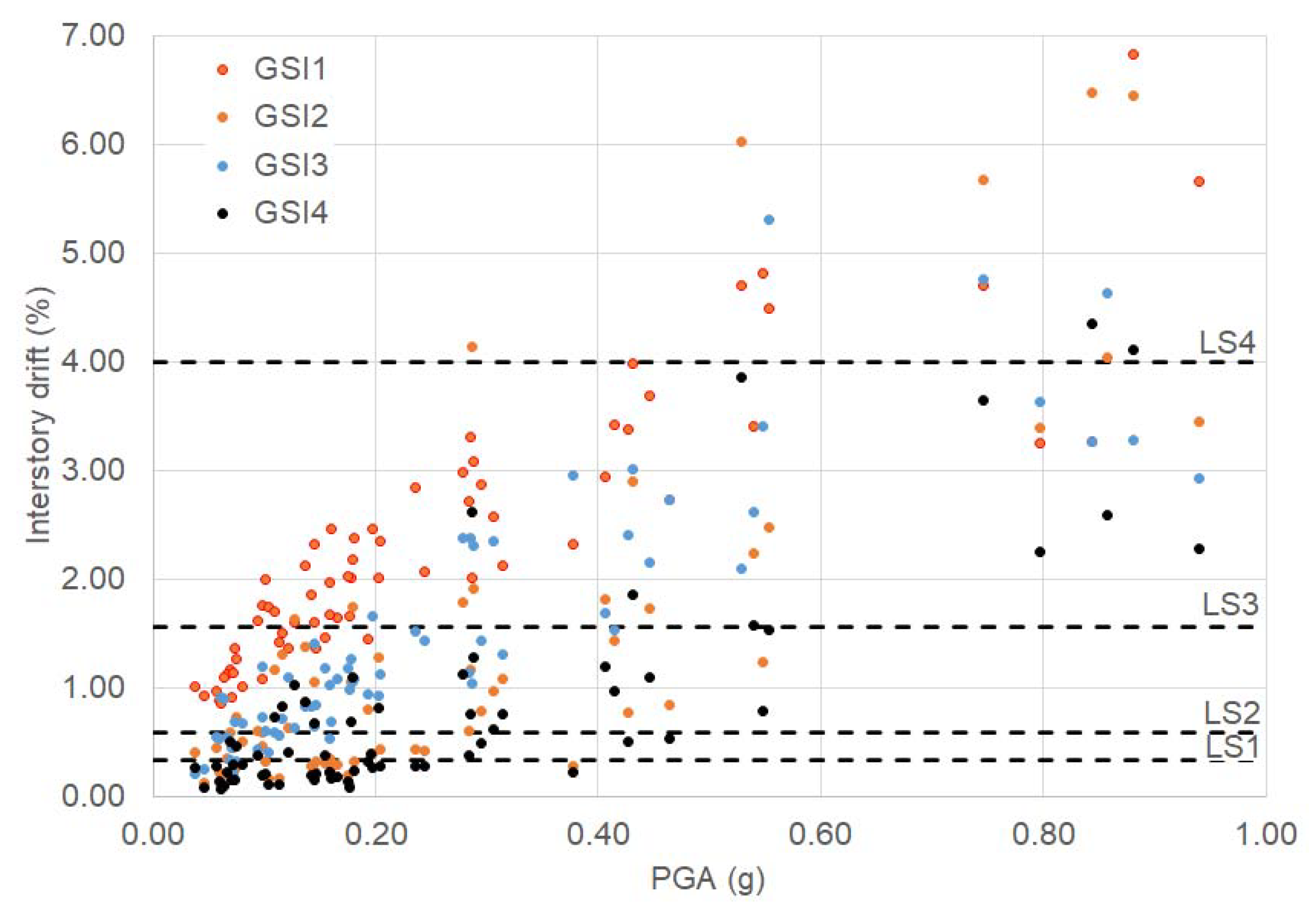
1] where the capacity of the GSI was compared with the convectional foundation without considering any isolation approach, this section investigates the effects of several the location of the liner by comparing the four selected configurations. In particular,
Figure 3 shows the results in terms of column drift (at the top of the structure) and PGA for GSI1, GSI2, GSI3 and GSI4. R
2 was chosen to evaluate the correlations between the results (PGA Vs maximum interstory drifts) and thus demonstrating a good correlation for all the configurations (
Table 6).
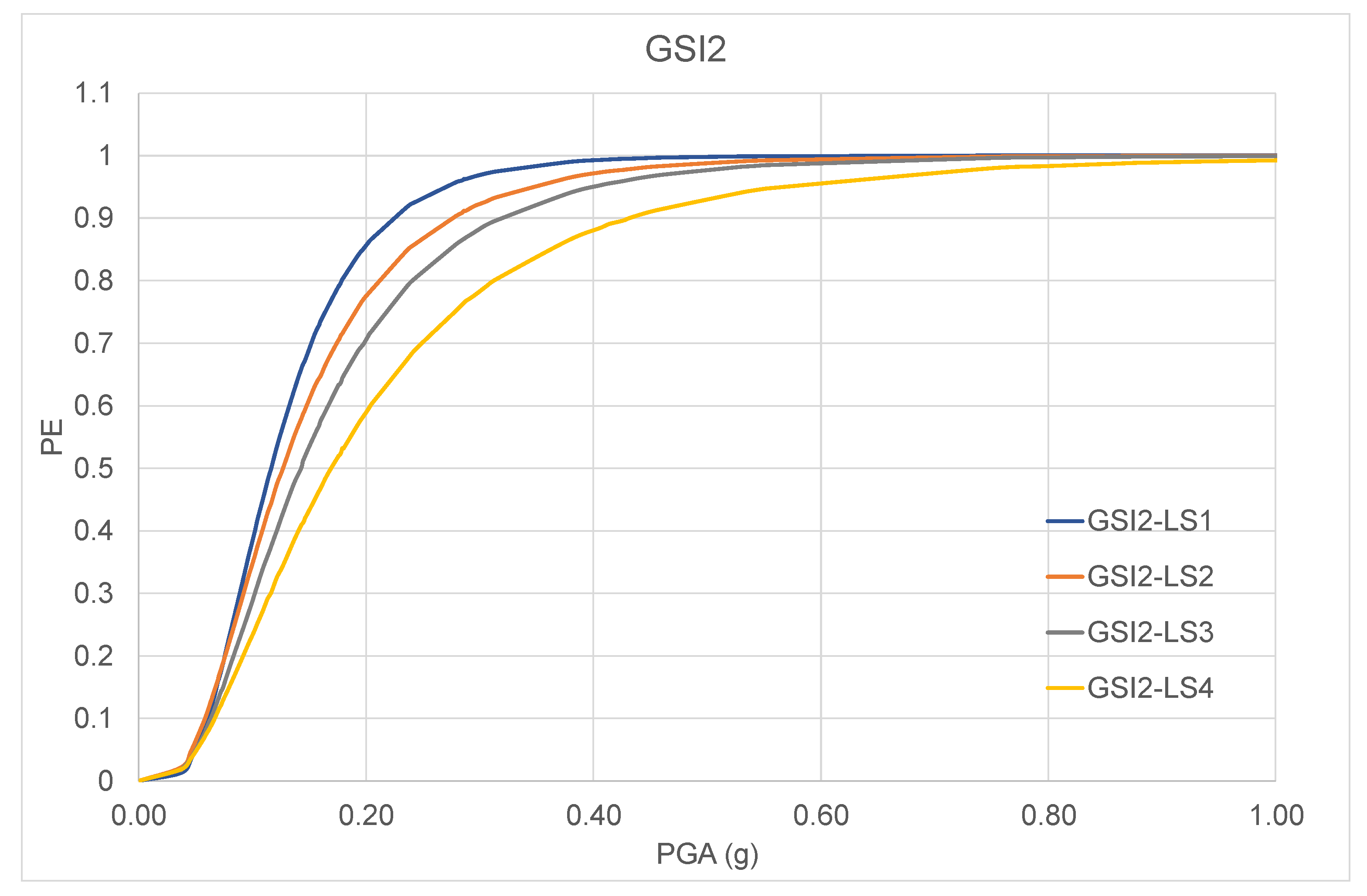
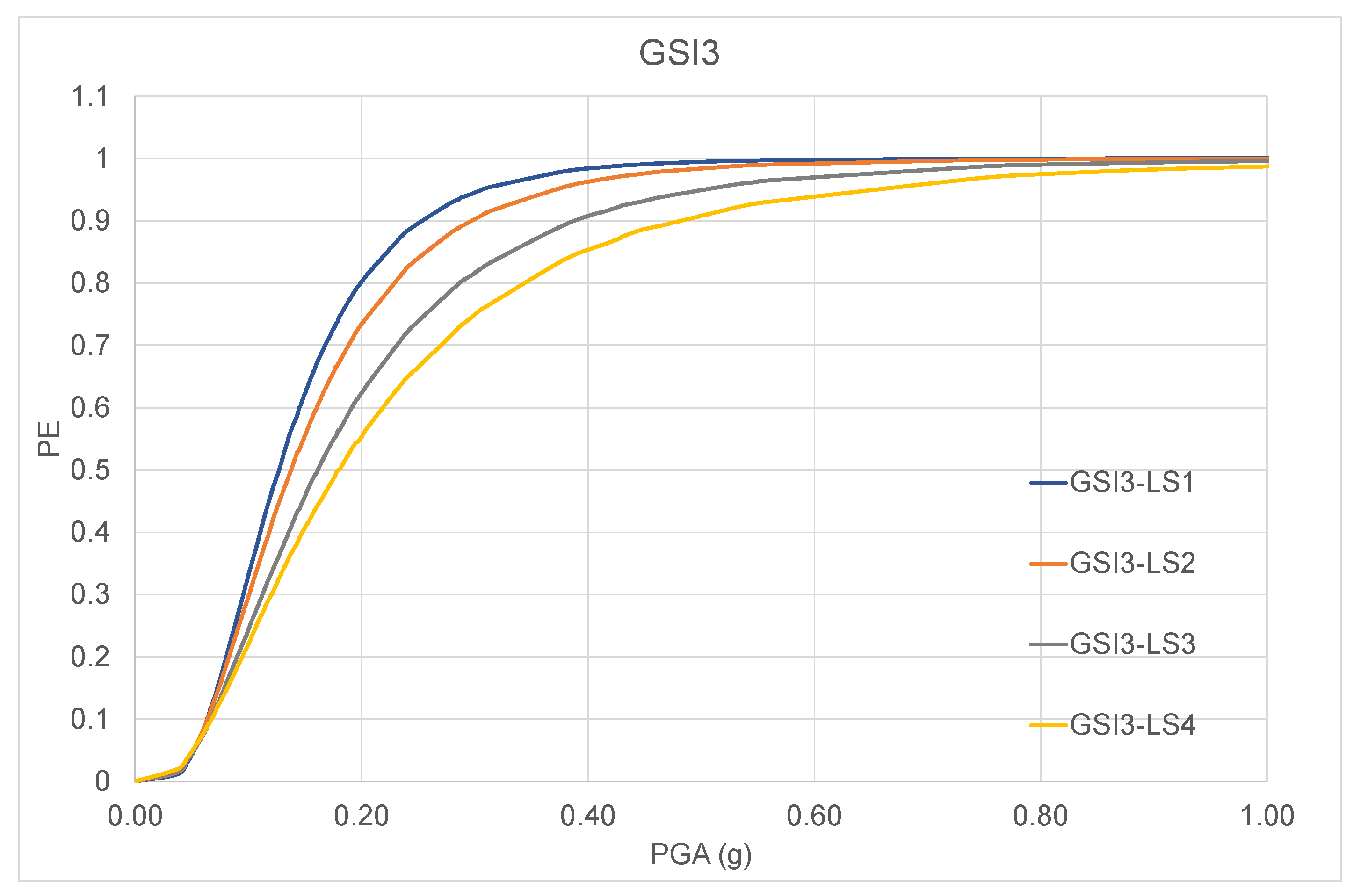
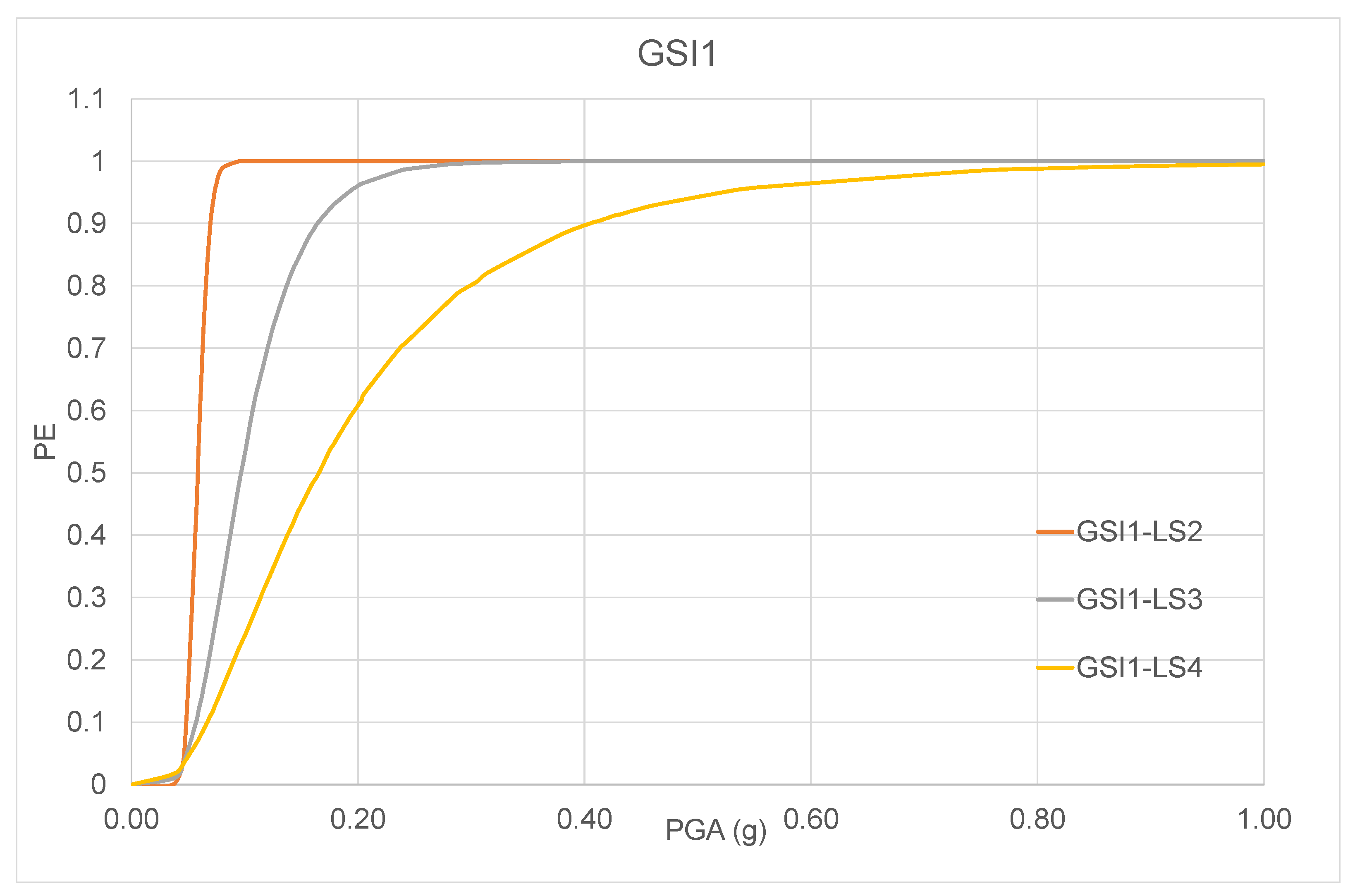
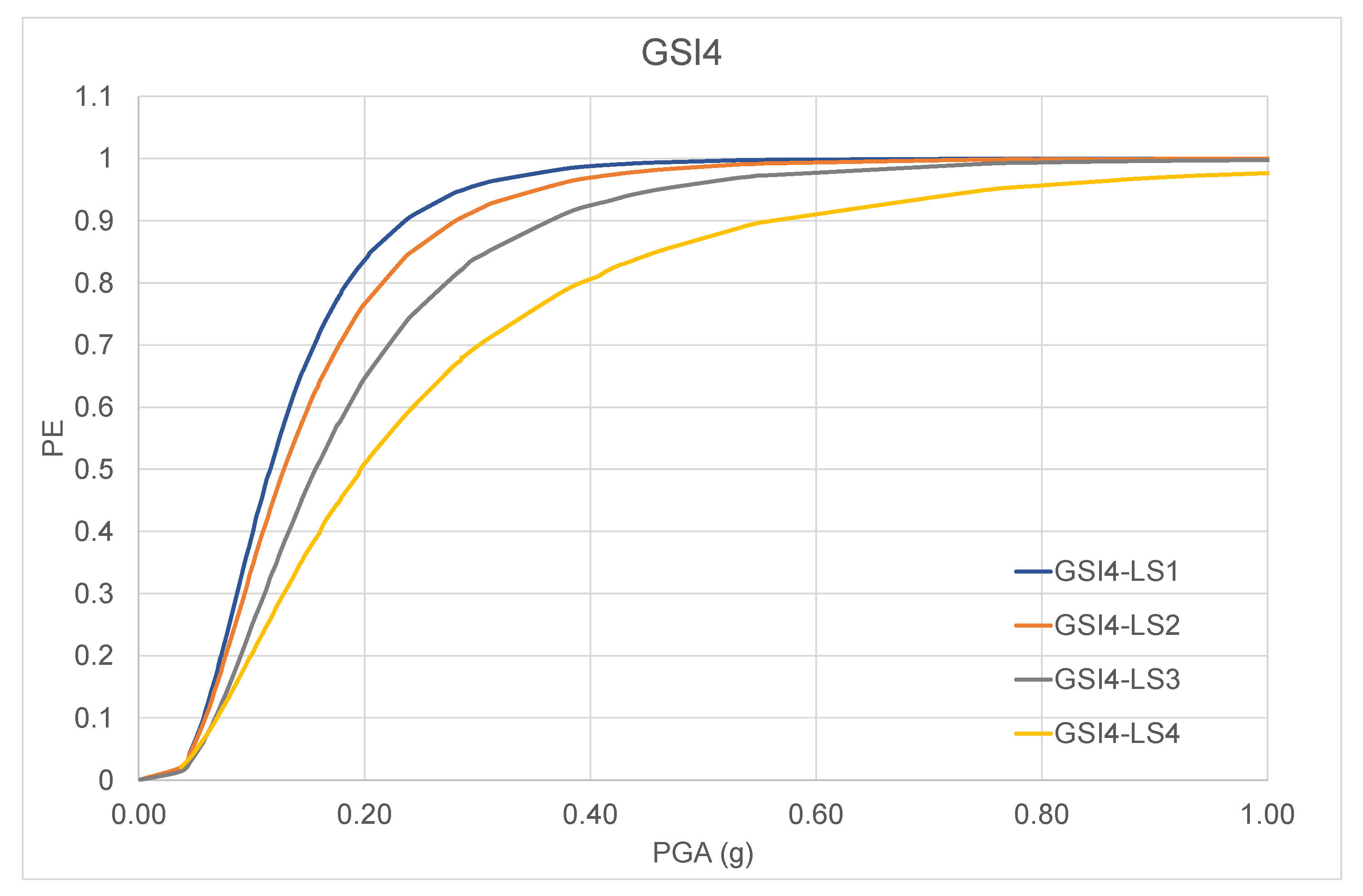
The linearization procedures allowed to calculate the values of the mean and the standard deviation for all the considered cases and developing analytical fragility curves, shown in
Figure 4,
Figure 5,
Figure 6 and
Figure 7 for the selected limit states (LS1, LS2, LS3 and LS4) that display the relationship between PGA (g) and the probability of exceedance (PE). Note that for GSI1 (
Figure 4), the level of damage is high and thus LS1 (slight damage) is not reached, demonstrating that the superficial location if GSI (configuration GSI1) does not help in reducing the damage to the structure and thus should be avoided.
Figure 5,
Figure 6 and
Figure 7 show that all the damage limits are reached, demonstrating that the most detrimental configuration is GSI1, when the liner is superficial [
1].
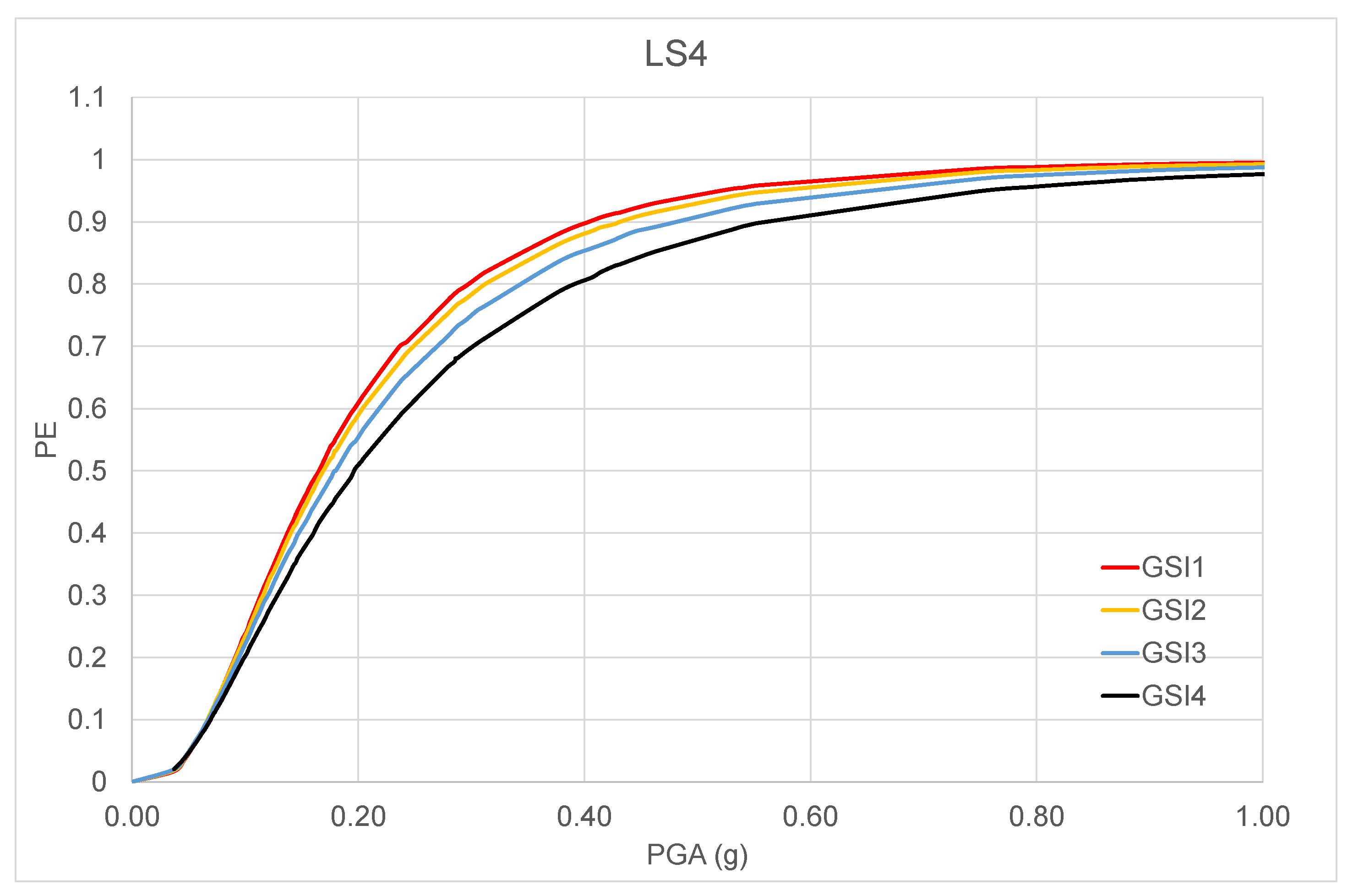
Figure 8 shows the comparison between the fragility curves for all the configurations for LS4 (complete damage, drift: 4%). In particular, the probability of exceedance (PE) varies with the location of the liner demonstrating the effect of the depth in reducing the damage among the entire range of PGA and at all the damage states. The differences between the configurations increases gradually as the severity of the motion increases, as shown in
Table 7 that compares the values of PE for increasing intensities: 0.20 g, 0.40 g and 0.60 g. In particular, when PGA = 0.40 g, PE are 0.900, 0.885, 0.858 and 0.810, respectively, for GSI1, GSI2, GSI3 and GSI4, demonstrating that fragility curve shift toward more fragile when the depth of the liner reduces. Therefore, it is important for design purposes to consider that the most vulnerable configuration is GSI1, where the liner is superficial. Therefore, the optimal configuration needs to be a compromise between costs (deeper liners mean higher costs) and effectiveness.
6. Conclusions
3D numerical analyses have been conducted to assess the response of four GSI configurations with liners at increasing depths. The study focused on reproducing 70 input motions with several intensities in order to follow a probabilistic-based approach that may account of many uncertainties. Analytical fragility curves were developed to assess the role of liner position in reducing the damage to the structure in terms of interstory drifts. Four limit states (slight, moderate, extensive, complete) were considered and defined as 0.33%, 0.58%, 1.56% and 4%, respectively. The results allow several important considerations.
Developing fragility curves was necessary in order to apply a probabilistic-based approach that allows to consider the uncertainties that are connected with the problem: soil characterization, earthquakes definition, structural model and choice of the damage indicators.
The vulnerability of the system depends on many factors, such as the coupled behaviour of the structure and the isolation. In this regard, applying a high nonlinear 3D numerical model was fundamental to realistically represent the complex mechanisms due to SSI.
The role of the location of the liner to reduce the damage and thus the vulnerability of the system (soil + structure) to earthquake motions. In particular, this outcome may be potentially applied to develop code prescriptions.
From a design point of view, it is fundamental to consider two important aspects: costs (that increase with the depth of the liner) and GSI effectiveness that was demonstrated to depend on the position of the liner. The deeper the position of the liner is, the less vulnerable the system becomes, thanks to the role of GSI in decoupling the ground from the superstructure.
Finally, note that these results are limited to the proposed case studies. However, they may have interesting applications for the design of GSI configurations.


