Real-Time Implementation of Robust Loop-Shaping Controller for a VSC HVDC System

Abstract

Voltage source converter (VSC) based HVDC systems are one of the most promising technologies for high voltage bulk power transmission. The reliability and stability of a VSC-based HVDC system greatly depends on the design of a proper controller for the inner decoupled d-q current loop. One of the major causes of instability in a properly tuned controller is due to system parameter variation. This paper presents the design of a fixed parameter robust controller for the inner decoupled d-q current loop for a VSC-based HVDC system to deal with the uncertainties due to system parameter variations. The method of multiplicative uncertainty is employed in the robust design to model the variations in the system parameters. The robust control design was realized through a graphical procedure known as the loop-shaping technique. The graphical loop shaping technique is a much simpler and more straightforward method compared to the traditional H∞-based algorithms for robust controller design. The designed robust controller was experimentally verified using a real-time hardware in loop (HIL) system and was tested on a VSC HVDC system. The performance of the designed robust controller is compared to that of a traditional PI controller. It has been observed that a classical PI controller is effective for a given operating point, and its performance deteriorates when the operating point changes or when the system parameters change. The studies conducted using real-time hardware in the loop (HIL) system prove that the designed loop-shaping-based robust controller provides very good performance and stability for a wide range of system parameter variations, such as changes in resistance and the inductance of the VSC HVDC system compared to the PI controller tuned using conventional methods.

1. Introduction

High Voltage Direct Current (HVDC) transmission is used to transmit bulk power over long distances or to connect two asynchronous AC networks. Traditionally, line commutated converters (LCC) based on thyristor technology have been employed for HVDC transmission systems [1]. Modern HVDC systems are based on voltage source converters (VSC) and use fast-acting Insulated Gate Bipolar Transistor (IGBT) switching technology. IGBT switches that constitute the building blocks of the VSC-based HVDC system enable the independent and fast control of active and reactive power. Additionally, the voltage source converters show good dynamic performance over a wide range of operating points. The world’s first VSC-based HVDC system was installed in 1997 and since then, many more have been installed worldwide [2]. VSC-based HVDC systema employ converter topologies that are either two-level or multi-level. Important future application fields that are best met by using VSC-based HVDC systems are power transmission to oil or gas platforms from land, power transmission and distribution from offshore wind farms to land, and as an improved and upgraded power supply for megacities [3,4] In these applications, the converters must be able to stabilize an AC-grid of relatively low short circuit power through the fast and independent control of the active and reactive power flow [5].

The control topologies used for VSC-based HVDC systems can be broadly classified into the Direct Power Control (DPC) and the Vector Oriented Control (VOC). DPC is simple to implement compared to VOC but exhibits varying switching frequency ripples in the output power [6]. Vector control based on the d-q reference frame model is the widely used in closed-loop control methods for VSC-based HVDC systems because of its good steady-state performance, constant switching frequency, and quick response [6]. In this paper, the VOC strategy is employed. This approach uses two cascade controllers—inner current controllers and outer voltage or reactive power and DC bus voltage or active power controllers. The inner and current controllers will be fast-acting to achieve the desired dynamic response. Many studies have been conducted by several authors to design controllers for VSC-based HVDC systems. Normally, these control strategies employ PI controllers tuned by pole-zero cancellation techniques based on a simplified single order model of the system. Multivariable optimal control of HVDC transmission links with network parameter estimation for weak grids is proposed by Beccuti et al. [7]. The First Order Plus Time Delay (FOPTD) model is used to develop a quasi-optimum PI control tuning algorithm for controlling the loops in VOC is presented by Taha et al. [8]. The authors Faisal et al. proposed a time-domain particle swarm optimization approach to design PI controllers for VSC-based bi-directional HVDC light systems [9]. The authors Jatin K. Pradhan et al. designed a multi-variable PI controller for a VSC-based HVDC transmission link [10]. These methods are simple, but the controller operates best at the designed operating point and does not guarantee robust performance.

Even though the PI controller is simple to tune and easy to implement, it only guarantees stability in the vicinity of a small operating region. However, the large-scale integration of renewable resources in a modern power system has the added extra uncertainty to the power system. As stipulated by the CIGRE B4-70 working group (Guide for Electromagnetic Transient Studies involving VSC converters [11]), the HVDC must be stable for large disturbances and wide changes in system parameters. As such, controllers need to be robust. A robust nonlinear controller for a VSC–HVDC transmission link using input–output linearization and a sliding mode control strategy is presented by Moharana et al. [12]. The authors Tang et al. propose a robust sliding mode controller for the active power modulation of a multi-terminal HVDC transmission system [13]. The major drawback of these methods is the chattering problem, and the implementation is also complex.

Several research papers have been reported in the literature for designing robust controllers based on the H∞ approach for a VSC-based HVDC system [14,15,16]. Robust nonlinear control strategies employing the H∞ approach are investigated and a state feedback robust H∞ controller is designed for transient stability enhancement of a VSC–HVDC system by Nayak et al. [15]. The H∞-based robust control design approach is an appealing technique, as it addresses the problem of model uncertainty. However, this method is mathematically too complex and involves non-linear modeling. Robust and generic control of full-bridge modular multilevel converter HVDC transmission systems is presented by Adam et al. [16]. The other attempts to design robust controllers for the VSC-based HVDC have been reported in the literature, but most of these approaches have been tested at a system level and not on the device level for tuning the inner decoupled d-q current loop of the VSC converters [16].

This article presents the design of a robust controller for the inner decoupled d-q current loop of a VSC-based HVDC system. The graphical loop-shaping technique is used to design a robust controller. Unlike H∞-based approach, this method is simple and intuitive. An uncertainty profile of the perturbed plant transfer functions was created by considering the degradation of the system parameter values from a nominal case, and the worst-case scenario of losing one transmission line for maintenance was also considered during the design procedure. In this scenario, the total system resistance and the total system inductance change, hence changing the system transfer function. For the first time, a robust controller design for VSC-based HVDC using the loop-shaping technique is presented. Additional contributions are variations in the switching frequency were also taken into account while building the uncertainty profile. Even though the proposed method can be applied to any grid-connected AC/DC converter and also to DC/AC converter, in this paper, the HVDC system is taken for study, as the HVDC system represents the most general case of a VSC system in which both AC/DC and DC/AC VSC converters are present with bi-directional power flow. The proposed robust controller is implemented on a dSpace platform in MATLAB/Simulink (Control Desk 7.3, 2020, dSpace GmbH, Germany) and is tested on a bi-directional HVDC system built on Typhoon real-time simulator (HIL-604, ver 2021.1 sp 1, Typhoon HIL GmbH, Baden, Switzerland). The system description and system model are presented in Section 2. A robust control design employing the graphical loop-shaping technique is discussed in detail in Section 3. The robustness of the system is verified through simulation, and the simulation results are presented in Section 4. The experimental results conducted on the Typhoon real-time simulator are given in Section 5. Finally, the conclusions are given in Section 6.

2. VSC HVDC System

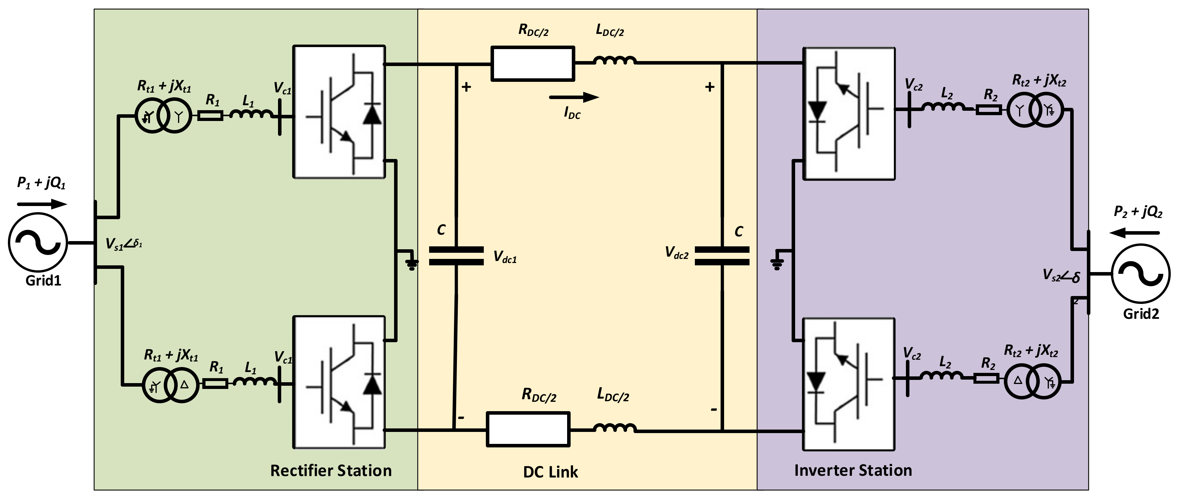
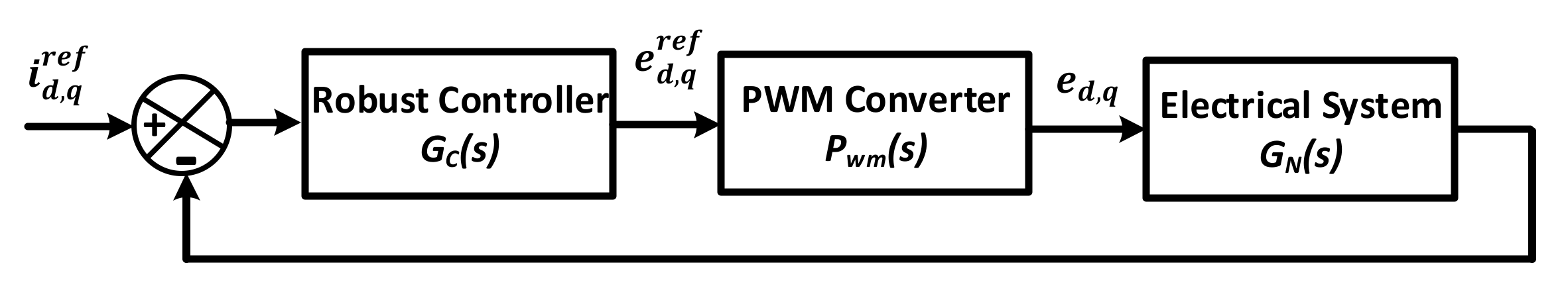
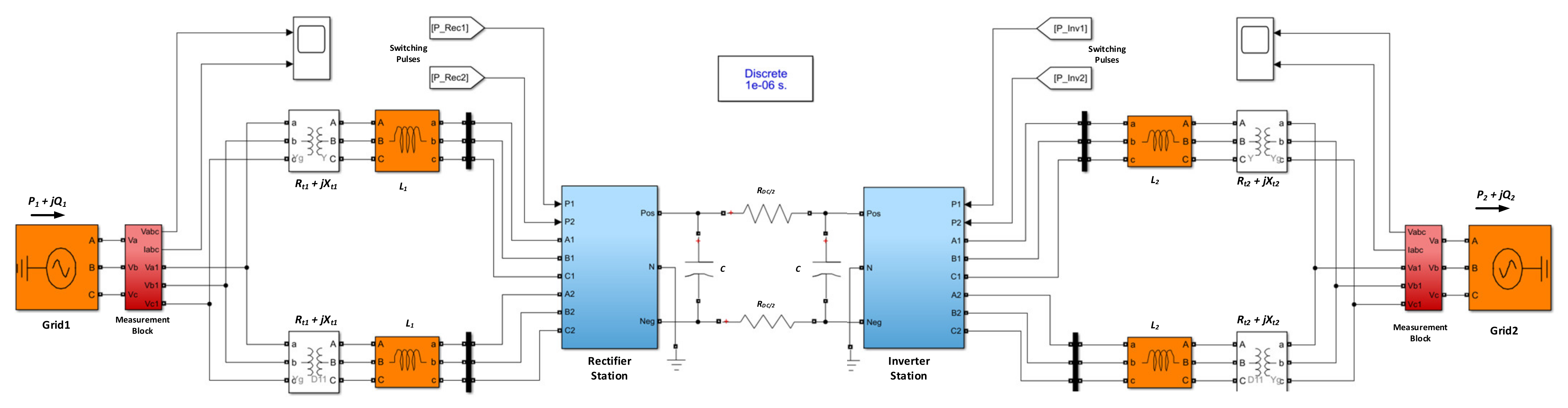
The VSC HVDC system shown in Figure 1 comprises a DC link, two converter stations, and two AC grids on either side. Each of these converters is a bi-polar VSC with neutral grounding. The AC transformers and grid filters form a connection between the grid and the DC link. The main purpose of the grid filters is to facilitate the transfer of power between the grid and the converters. The grid filters also help in suppressing the high-frequency harmonics in the line currents. The power from one AC grid to the other is transferred through the DC link. The role of the capacitors on the DC side of the converters is to provide voltage support and to attenuate the DC voltage harmonics. The VSC-based HVDC system shown in Figure 1 is capable of bi-directional power flow. When the power flows from Grid-1 to Grid-2, converter-1 acts as a rectifier, whereas converter-2 acts as an inverter, and vice versa. Under normal operation, the ground conductors carry no current, thereby preventing corrosion in the ground conductors. In case of an outage of one of the two poles, the system can still be operated as a mono-polar system with reduced capacity. The detailed mathematical model of the VSC HVDC system and the control loops of the inverter and rectifier stations are discussed in the following sections.

2.1. Mathematical Model of the System in d-q Reference Frame

The rectifier and the inverter stations of the VSC HVDC system of Figure 1 comprise of three-phase, three-level, six pulse bridge converters. The power electronic devices used in each converter are self-commutating IGBT switches with anti-parallel diodes. The nominal parameters of the VSC HVDC system are given in

Table 1. ^* VSC HVDC System Parameters.

Parameter	Symbol	Value
System rating	S	50 MVA
System frequency	f	50 Hz
Grid Line voltage	Vs	110 kV
Transformer voltage	Vt	110 kV/33 kV
Transformer reactance	Xt	9%
Transformer X/R ratio	Xt/Rt	6.63
Grid filter	L	15 mH
DC-link voltage	Vdc	±200 kV
DC capacitor	C	200 µF
DC line resistance	Rdc	0.1 Ω/km (100 km)
Switching frequency	fsw	2850 Hz

^* Superscript * refers to Converter 1 (rectifier) and subscript 2 refers to Converter 2 (inverter).For this study, it is assumed that both the converter stations have identical parameters.

. The system parameters of Tabel 1 are adapted from Pradhan et al. [10]. Both the rectifier and inverter station are connected to the AC grids via equivalent impedances $Z_1=R_1+j\omega L_1$ and $Z_2=R_2+j\omega L_2$ respectively. R₁ and R₂ represent the total resistance of the transmission line and the filter, and L₁ and L₂ represent the total inductance of the transmission line and the filter. In Figure 1, subscript 1 refers to Converter 1 (rectifier), and subscript 2 refers to converter 2 (inverter). It is assumed that $R_1=R_2=R$ and $L_1=L_2=L$. Both the converters are assumed to be tied to strong AC grids, so any coupling arising from the dynamics between the PLL and control loops is not considered during the modeling of the VSC HVDC system. The dynamic equations governing the rectifier and the inverter stations of the system shown in Figure 1 in the rotating d-q reference frame are given by authors Faisal et al. [9]:

Rectifier Station:

$$\left[\begin{array}{c}{V}_{sd1}\\ V_{sq1}\end{array}\right]=R_1\left[\begin{array}{c}{i}_{d1}\\ i_{q1}\end{array}\right]+L_1\frac{d}{dt}\left[\begin{array}{c}{i}_{d1}\\ i_{q1}\end{array}\right]+\omega L_1\left[\begin{array}{c}-i_{q1}\\ i_{d1}\end{array}\right]+\left[\begin{array}{c}{V}_{cd1}\\ V_{cq1}\end{array}\right]$$

(1)

Inverter Station:

$$\left[\begin{array}{c}{V}_{sd2}\\ V_{sq2}\end{array}\right]=R_2\left[\begin{array}{c}{i}_{d2}\\ i_{q2}\end{array}\right]+L_2\frac{d}{dt}\left[\begin{array}{c}{i}_{d2}\\ i_{q2}\end{array}\right]+\omega L_2\left[\begin{array}{c}-i_{q2}\\ i_{d2}\end{array}\right]+\left[\begin{array}{c}{V}_{cd2}\\ V_{cq2}\end{array}\right]$$

(2)

In the synchronous reference frame, $V_{sd1}, V_{sq1}, V_{sd2}, V_{sq2}, i_{d1}, i_{q1}, i_{d2},$ and $i_{q2}$ are d and q axis components of instantaneous source voltages and currents, and $V_{cd1}, V_{cq1}, V_{cd2},$ and $V_{cq2}$ are converter voltages along the d and q axes; ω is the angular frequency of the AC grid, $R_1$ and $R_2$ represent the total line resistance, and $L_1$ and $L_2$ represent the total line inductance from the converter to the AC grid. $P_1, P_2, Q_1$, and $Q_2$ are the active and reactive power flowing from the AC grid to the converter stations, $V_{DC1}$ and $V_{DC2}$ are the dc bus voltages, and $I_{DC}$ is the DC link current.

Aligning the d-axis of the reference frame with the voltage of the AC grid results in constant d-axis and zero q-axis voltage components. Therefore, Equations (3) and (4) give the instantaneous AC active and reactive powers, respectively,

$$P_1=\frac{3}{2}\left(V_{sd1}{i}_{d1}+V_{sq1}{i}_{q1} \right)=\frac{3}{2}{V}_{sd1}{i}_{d1}$$

(3)

$$Q_1=\frac{3}{2}\left(V_{sq1}{i}_{d1}-V_{sd1}{i}_{q1} \right)=-\frac{3}{2}{V}_{sd1}{i}_{q1}$$

(4)

The two converter stations are connected via a DC link. To simplify the DC circuit analysis, the effect of line inductance on the DC side is neglected. The DC power balance equation for the DC link is given by:

$$P_{dc1}=V_{dc1}{i}_{dc}=V_{dc2}{i}_{dc}+2R_{dc}{i}_{dc}^2$$

(5)

Assuming that there is no power loss at the converter stations, the AC power is equal to the DC power as given by:

$$P_1=P_{dc1}=\frac{3}{2}{V}_{sd1}{i}_{d1}=V_{dc1}{i}_{dc1}$$

(6)

The dynamics of the $v_{dc1}$ are given by:

$$i_{dc1}=C\frac{d{v}_{dc1}}{dt}+\frac{v_{dc1}}{R_{load}}$$

(7)

where $R_{load}$ is the Thevenin equivalent load resistance of the load seen from the DC terminals of the rectifier, and C is the DC link capacitance.

Substituting (6) in (7), the $v_{dc1}$ dynamics can be written in terms of $i_{d1}$ as they are in (8)

$$\frac{3}{2}\frac{V_{sd1}}{V_{dc1}}{i}_{d1}=C\frac{d{v}_{dc1}}{dt}+\frac{v_{dc1}}{R_{load}}$$

(8)

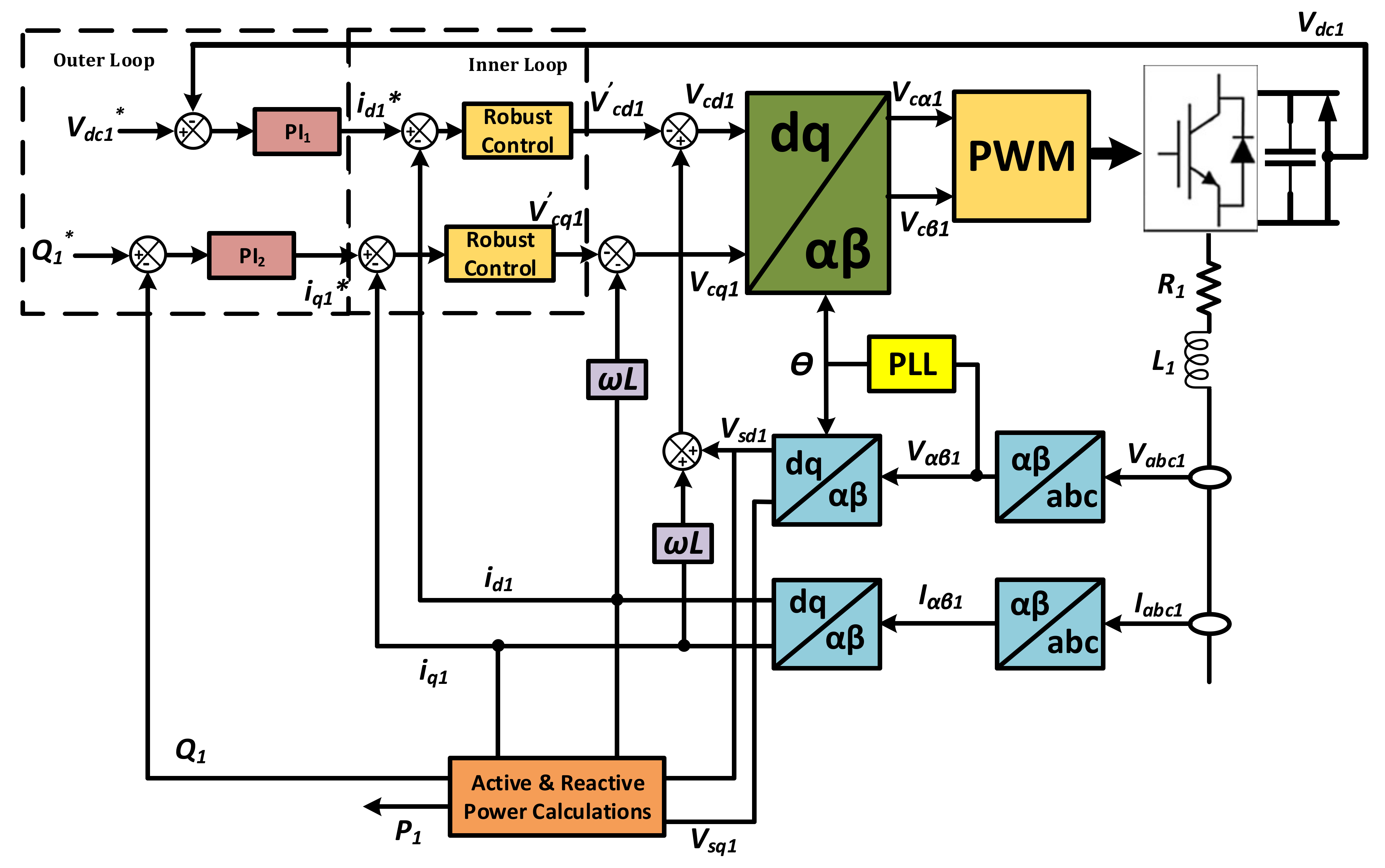
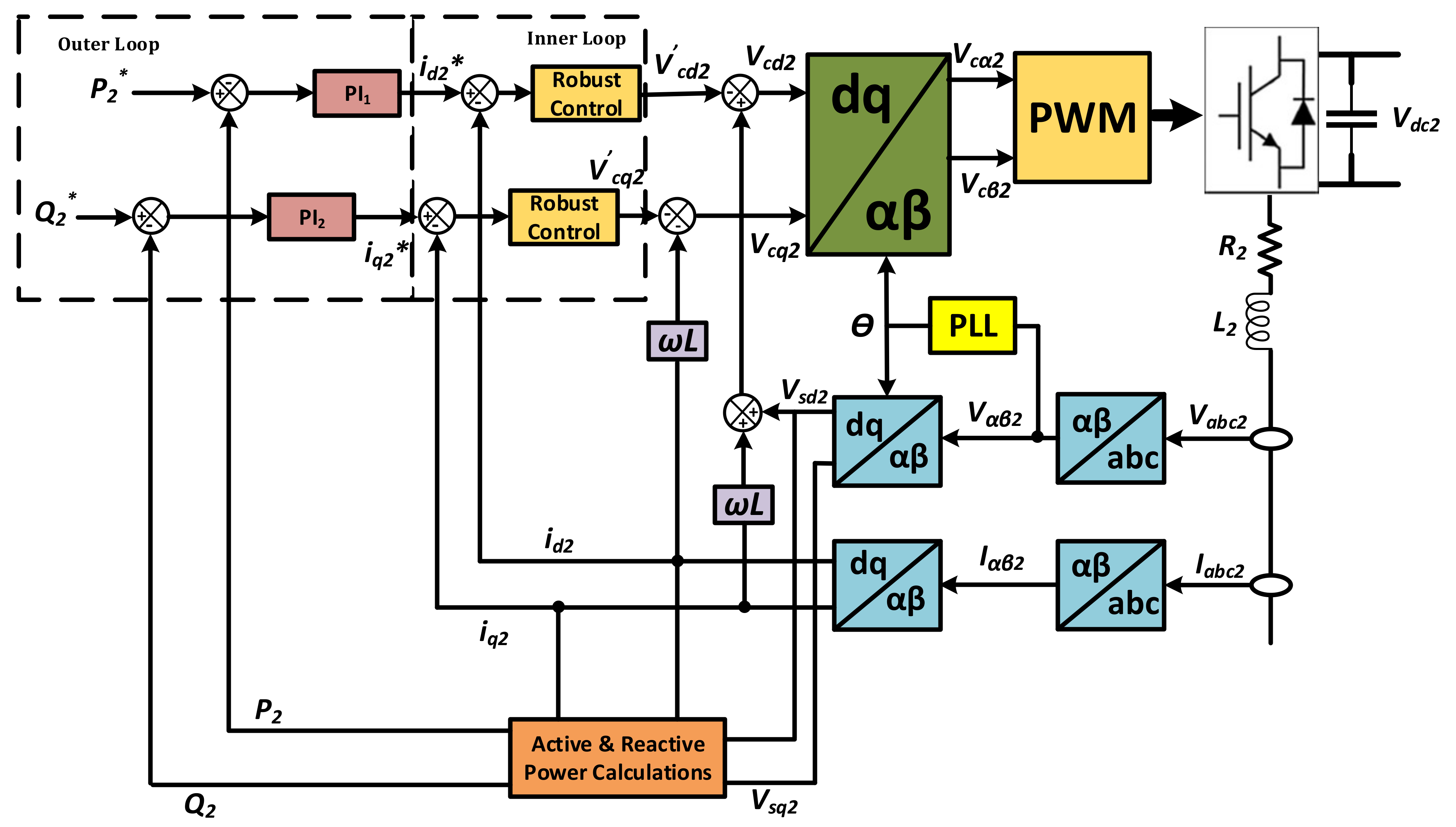
2.2. Control Loops of the VSC HVDC Light System

For the case study in this paper, a Vector Oriented Control (VOC) approach is used. VOC utilizes the decoupled d-q control scheme, has two nested control loops, a relatively faster inner loop that controls the d-q components of the current, and a slower outer loop. The coupling terms ($L_1\omega i_{q1},L_1\omega i_{d1}, L_2\omega i_{q2}, and L_2\omega i_{d2},$) in Equations (1) and (2) are decoupled through feed-forward inputs as seen in Equations (9) and (10).

$$\left[\begin{array}{c}{V}_{xd1}\\ V_{xq1}\end{array}\right]=R_1\left[\begin{array}{c}{i}_{d1}\\ i_{q1}\end{array}\right]+L_1\frac{d}{dt}\left[\begin{array}{c}{i}_{d1}\\ i_{q1}\end{array}\right]$$

(9)

where, $\left[\begin{array}{c}{V}_{xd1}\\ V_{xq1}\end{array}\right]=\left[\begin{array}{c}{V}_{sd1}\\ V_{sq1}\end{array}\right]-\omega L_1\left[\begin{array}{c}-i_{q1}\\ i_{d1}\end{array}\right]-\left[\begin{array}{c}{V}_{cd1}\\ V_{cq1}\end{array}\right]$

$$\left[\begin{array}{c}{V}_{xd2}\\ V_{xq2}\end{array}\right]=R_2\left[\begin{array}{c}{i}_{d2}\\ i_{q2}\end{array}\right]+L_2\frac{d}{dt}\left[\begin{array}{c}{i}_{d2}\\ i_{q2}\end{array}\right]$$

(10)

where, $\left[\begin{array}{c}{V}_{xd2}\\ V_{xq2}\end{array}\right]=\left[\begin{array}{c}{V}_{sd2}\\ V_{sq2}\end{array}\right]-\omega L_2\left[\begin{array}{c}-i_{q2}\\ i_{d2}\end{array}\right]-\left[\begin{array}{c}{V}_{cd2}\\ V_{cq2}\end{array}\right]$

The dynamic Equations (9) and (10) are first-order systems and can be compensated using the linear compensator design techniques.

The block diagrams showing the decoupled d-q control scheme for the rectifier and the inverter stations are shown in Figure 2 and Figure 3, respectively. The outer control loop provides the setpoints to the inner current control loop. In this paper, the control objective is active power (P) control, reactive power (Q) control, and DC link voltage (V_dc) control. For power flow from Grid 1 to Grid 2, the P, Q, and V_dc control are realized using the classical PI controllers, as shown in Figure 2 and Figure 3. The inner decoupled d-q current loop is realized using a robust controller.

3. Robust Controller Design by Graphical Loop Shaping

The robust control design problem for the inner d-q current loop for the VSC HVDC system can be stated as: given a set of Equations (9) and (10), design a controller that will stabilize the nominal system following a disturbance. If the designed controller can also stabilize the VSC HVDC system for the other operating conditions in the vicinity of the nominal conditions, then the design objectives for robust control are met.

The VSCH VDC system of Figure 1 must be stable over a wide range of operating conditions, as disturbances of differing extents of severity could happen during the normal operations, and the topology of the system could change over time. The existence of uncertainties requires good robustness of the control system. The changes in the system parameters of the VSC HVDC system can be viewed as changes in the coefficients of the system nominal plant transfer function G_N and are considered as model uncertainty. In this paper, these changes are modeled as multiplicative uncertainties, and the robust design procedure is applied to arrive at a robust controller.

The robust controller design starts by obtaining the nominal plant transfer function G_N by rewriting the Equations (9) and (10) for the inner d-q current loop as

$$\left[\begin{array}{c}{V}_{cd1}\\ V_{cq1}\end{array}\right]=\left[\begin{array}{c}\left(R_1{i}_{d1}+L_1\frac{d{i}_{d1}}{dt}\right)-\omega L_1{i}_{q1}-V_{sd1}\\ \left(R_1{i}_{q1}+L_1\frac{d{i}_{q1}}{dt}\right)+\omega L_1{i}_{d1}\end{array}\right]$$

(11)

where the terms in normal brackets in Equation (11) are treated as state equations between the voltage and the current for the d-q axes current control loops, whereas the terms outside the normal brackets are treated as compensation terms. A similar equation can also be written for converter 2.

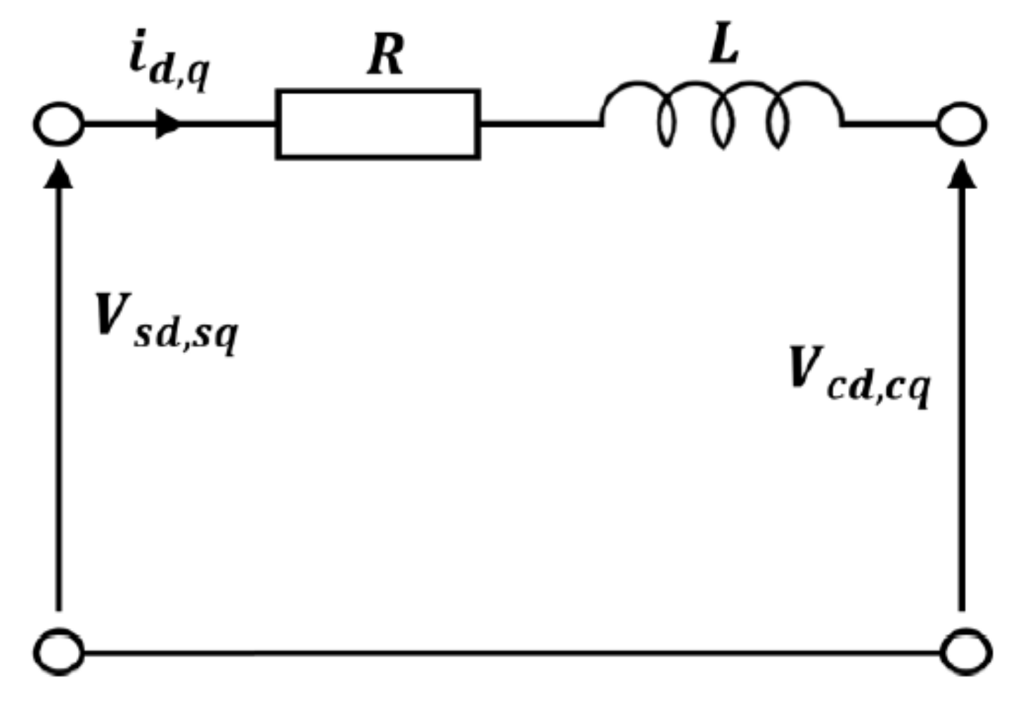
Hence, the $i_d$ and $i_q$ controller is designed based on the nominal plant transfer function G_N given by

$$G_N=\frac{i_d}{V_{xd}}=\frac{i_q}{V_{xq}}=\frac{1}{Ls+R}$$

(12)

where$V_{xd}=V_{cd}+\omega L{i}_q+V_{sd}$ and $V_{xq}=V_{cq}-\omega L{i}_d$ and R and L are the equivalent resistance and inductance of the grid and filter, respectively. Thevinin’s equivalent circuit realization for the inner d-q current loop for the VSC HVDC system is shown in Figure 4.

The changes in the system operating conditions and the system parameters can be considered as variations in the coefficients of the plant transfer function and can be represented by multiplicative uncertainties. The robust controller can then be designed for the ranges of perturbations or variations in the plant transfer function. The following subsections give a brief theory of uncertainty modeling, the robust stability criterion, a graphical designed technique termed loop-shapingand, and finally, the graphical loop-shaping algorithm is presented.

3.1. Uncertainty Model

Suppose G_N belongs to a bounded set of transfer functions and consider that due to changes in the system the perturbed plant transfer function $\widetilde{G_N}$ parameters can be expressed in the form

$$\widetilde{G_N}=\left(1+\Delta W_{f2}\right)G_N$$

(13)

where $W_{f2}$ is a weight function, and $\Delta$ is a variable transfer function satisfying ${\Vert \Delta \Vert }_{\infty }<1$. The infinity norm (∞-norm) of a function is the least upper boundary of its absolute value, also written as ${\Vert \Delta \Vert }_{\infty }=su{p}_{\omega }\left|\Delta \left(\mathrm{j}\omega \right)\right|$, is the largest value of gain on a Bode magnitude plot. The uncertainties, which are the changes in the system parameters or the operating points are thus modeled through $\widetilde{G_N}$ in (13). The feedback loop with uncertainty model representation is shown in Figure 5.

Equation (13) represents the multiplicative uncertainty model, and $\Delta W_{f2}$ is the normalized plant perturbations away from 1. If ${\Vert \Delta \Vert }_{\infty }<1$ then

$$\left|\frac{\widetilde{G_N}\left(j\omega \right)}{G_N\left(j\omega \right)}-1\right|\le \left|W_{f2}\left(j\omega \right)\right|\forall \omega$$

(14)

Therefore, $\left|W_{f2}\left(j\omega \right)\right|$ provides the uncertainty profile, and in the frequency plane, it is the upper boundary of all of the normalized plant transfer functions away from 1.

3.2. Robust Stability and Performance

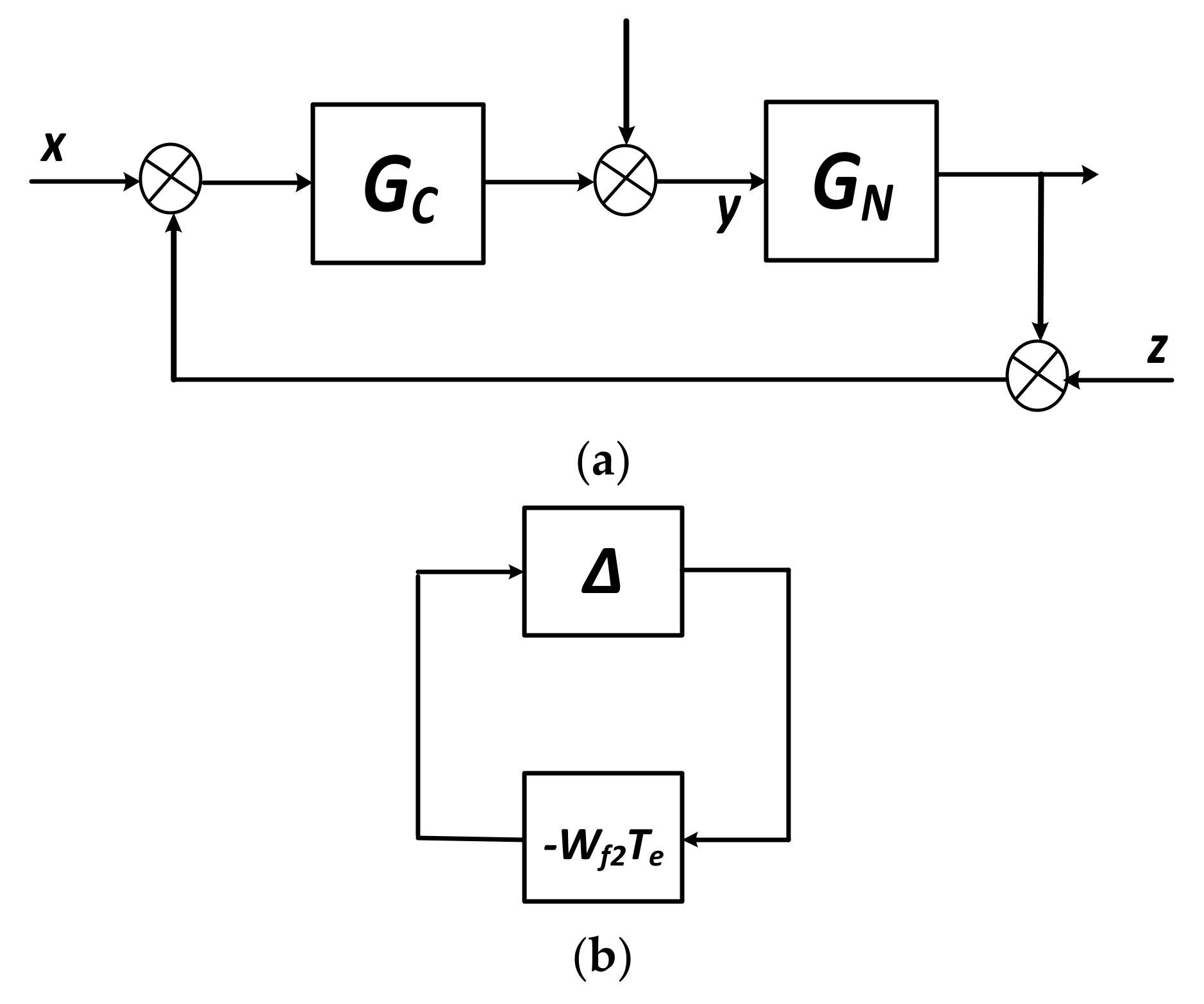
Considering the multi-input control system of Figure 6a, a controller $G_C$ provides robust stability if it provides internal stability for every plant in the uncertainty set. If $G_O$ denotes the open-loop transfer function ($G_O=G_{N{G}_C}$), then the sensitivity function is written as

$$S_e=\frac{1}{1+G_N}$$

(15)

The complementary sensitivity function or the input–output transfer function is given by

$$T_e=1-S_e=\frac{1}{1+G_o}=\frac{G_N{G}_C}{1+G_N{G}_C}$$

(16)

For a multiplicative perturbation model, the robust stability condition is met if and only if ${\Vert W}_{f2}{T}_e{\Vert }_{\infty }<1$. This implies that

$$\left|\frac{W_{f2}\left(j\omega \right)G_O\left(j\omega \right)}{1+G_O\left(j\omega \right)}\right|<1 \mathrm{for} \mathrm{all} \omega$$

(17)

or

$$\left|\Delta \left(\mathrm{j}\omega \right)W_{f2}\left(j\omega \right)G_O\left(j\omega \right)\right|<\left|1+G_O\left(j\omega \right)\right| \mathrm{for} \mathrm{all} \omega \mathrm{and} {\Vert \Delta \Vert }_{\infty }<1$$

(18)

The block diagram of a typical perturbed system, ignoring all inputs, is shown in Figure 5. The transfer function from the output of $\Delta$ to the input of $\Delta$ is equal to $W_{f2}{T}_e$. The properties of the block diagram can be reduced to those of the configuration given in Figure 6b.

The maximum loop gain $-{\Vert W}_{f2}{T}_e{\Vert }_{\infty }$ is less than 1 for all allowable $\Delta$if and only if the small gain condition ${\Vert W}_{f2}{T}_e{\Vert }_{\infty }<1$ holds. The nominal performance condition for an internally stable system is given as ${\Vert W}_{f1}{S}_e{\Vert }_{\infty }<1$, where $W_{f1}$ is a real–rational, stable, minimum phase transfer function, also called a weighting function. If $G_N$ is perturbed to $\widetilde{G_N}=\left(1+\Delta W_{f2}\right)G_N$, and $S_e$ is perturbed to

$$\widetilde{S_e}=\frac{1}{1+(1+\Delta W_{f2}{G}_N)}=\frac{S_e}{1+\Delta W_{f2}{T}_e}$$

(19)

The robust performance condition can therefore be written as

$${\Vert W}_{f2}{T}_e{\Vert }_{\infty }<1, \mathrm{and} {\Vert \frac{W_{f1}{S}_e}{W_{f2}{T}_e}\Vert }_{\infty }<1 \mathrm{for} \mathrm{all} {\Vert \Delta \Vert }_{\infty }<1$$

(20)

Combining the above equations, it can be shown that a necessary and sufficient condition for robust stability and performance is

$${\Vert W}_{f1}{S}_e+W_{f2}{T}_e{\Vert }_{\infty }<1$$

(21)

To summarize the above sections, it can be said that for a control function $G_C$ in cascade with the plant $G_N$, the robustness measures are,

a)

The nominal performance measure is ${\Vert W}_{f1}{S}_e{\Vert }_{\infty }<1$;

b)

G_C provides robust stability iff ${\Vert W}_{f2}{T}_e{\Vert }_{\infty }<1$;

c)

The necessary and sufficient condition for robust stability and robust performance is given by Equation (21).

3.3. The Loop-Shaping Technique

The loop-shaping technique is a graphical process to design a controller G_C fulfilling the robust performance and stability conditions given in Equations (20) and (21). The main idea of the loop shaping technique is to construct an open-loop transfer function, $G_O=G_N{G}_C,$ to satisfy the criteria given by Equations (22) and (23) and then to obtain the robust controller, $G_C=G_O /G_{N }$. The internal stability of the plant and the properness of $G_C$ constitute the constraints of the method. During the design process, care must be taken such that $G_N{G}_C$ should not have any pole-zero cancellation. An important criterion for robustness is that either or both $\left|W_{f1}\right|$, $\left|W_{f2}\right|$ must be less than 1.

$$\left|G_O\right|>\frac{\left|W_{f1}\right|}{1-\left|W_{f2}\right|} \mathrm{at} \mathrm{low} \mathrm{frequencies}$$

(22)

$$\left|G_O\right|<\frac{1-\left|W_{f1}\right|}{\left|W_{f2}\right|}\approx \frac{1}{\left|W_{f2}\right|} \mathrm{at} \mathrm{high} \mathrm{frequencies}$$

(23)

At high frequencies, the dB magnitude of the open-loop function $G_O$ should roll off at least as quickly as the dB magnitude of the plant transfer function $G_N$. This ensures the properness of the closed-loop system. The gain of the open-loop transfer function $G_O$ at low frequencies should be large enough, and the dB slope of $G_O$ should not be very steep near the crossover frequency to avoid internal instability [17,18,19,20,21].

3.4. Graphical Loop Shaping Algorithm

The general algorithm for the graphical loop-shaping design process can be summarized as:

 Step1: 

Construct the dB-magnitude plot for the nominal as well as perturbed plant transfer functions. These dB magnitude plots can be constructed by using Equations (12) and (13) respectively;

 Step2: 

Construct $W_{f2}$ satisfying the constraint given in Equation (14). It is to be noted here that $W_{f2}$ provides the uncertainty profile of the perturbed plant transfer functions;

 Step3: 

Fit a graph of the dB magnitude of the open-loop transfer function G_O, satisfying the constraints given in Equations (22) and (23);

 Step4: 

For the open-loop transfer function G_O, constructed in step 3, ensure that G_O is a stable minimum-phase transfer function and G_O(0) > 0. The latter condition guarantees negative feedback;

 Step5: 

Obtain the robust controller G_C from the relation G_O = G_NG_C;

 Step6: 

Check that the nominal stability and robust stability criteria of Equations (20) and (21) are satisfied;

 Step7: 

Verify that the closed-loop system with the controller is internally stable by direct simulation for pre-selected disturbances or inputs;

 Step8: 

Iterate through step 3 to step 7 until acceptable G_O and G_C are obtained. Note that a robust controller may not exist for all nominal conditions, and if it does, it may not be unique.

The steps of the graphical loop-shaping algorithm are illustrated in detail in the following section.

3.5. Implementation of Graphical Loop-Shaping Algorithm to VSC HVDC System

In this section, the graphical loop-shaping algorithm discussed in the previous section is implemented to design the robust controller for the inner decoupled d-q current loop of the VSC HVDC system of Figure 1. The control loop can be represented by a general block diagram, as shown in Figure 7. The plant output to be fed back to the robust controller G_C is chosen as the d-q current components of the grid. The system parameters shown in Table 1 are considered as the nominal system parameters.

The first step in the graphical loop-shaping algorithm is to construct the nominal and the perturbed plant transfer functions. The nominal plant transfer function considering the system parameters given in Table 1 can be constructed from Equation (12) and is given as

$$G_N=\frac{i_d}{V_{xd}}=\frac{i_q}{V_{xq}}=\frac{1}{Ls+R}=\frac{37.46}{\left(s+26.17\right)}$$

(24)

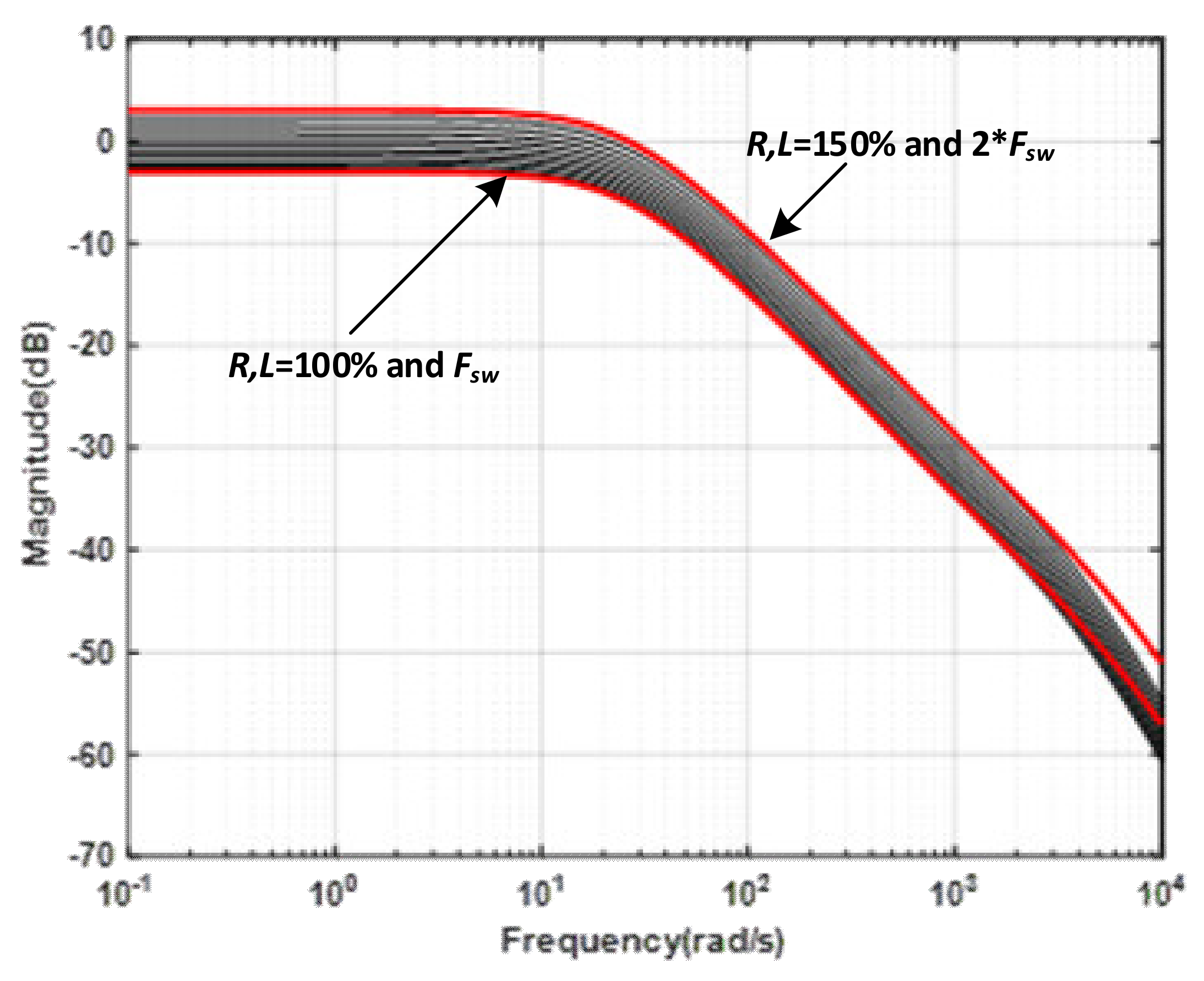
Equation (24) is used to construct the dB magnitude plot of the nominal plant transfer function, and the perturbed plant transfer functions are constructed by considering the degradation of system parameter (R and L) values due to aging and are considered as off-nominal system parameter variations. Variations between 100% and 150% were considered, and the worst-case scenario of one transmission line outage for maintenance was considered to create the dB magnitude plot of the perturbed plant transfer functions. The dB magnitude plots of the perturbed plant transfer functions are shown in Figure 8.

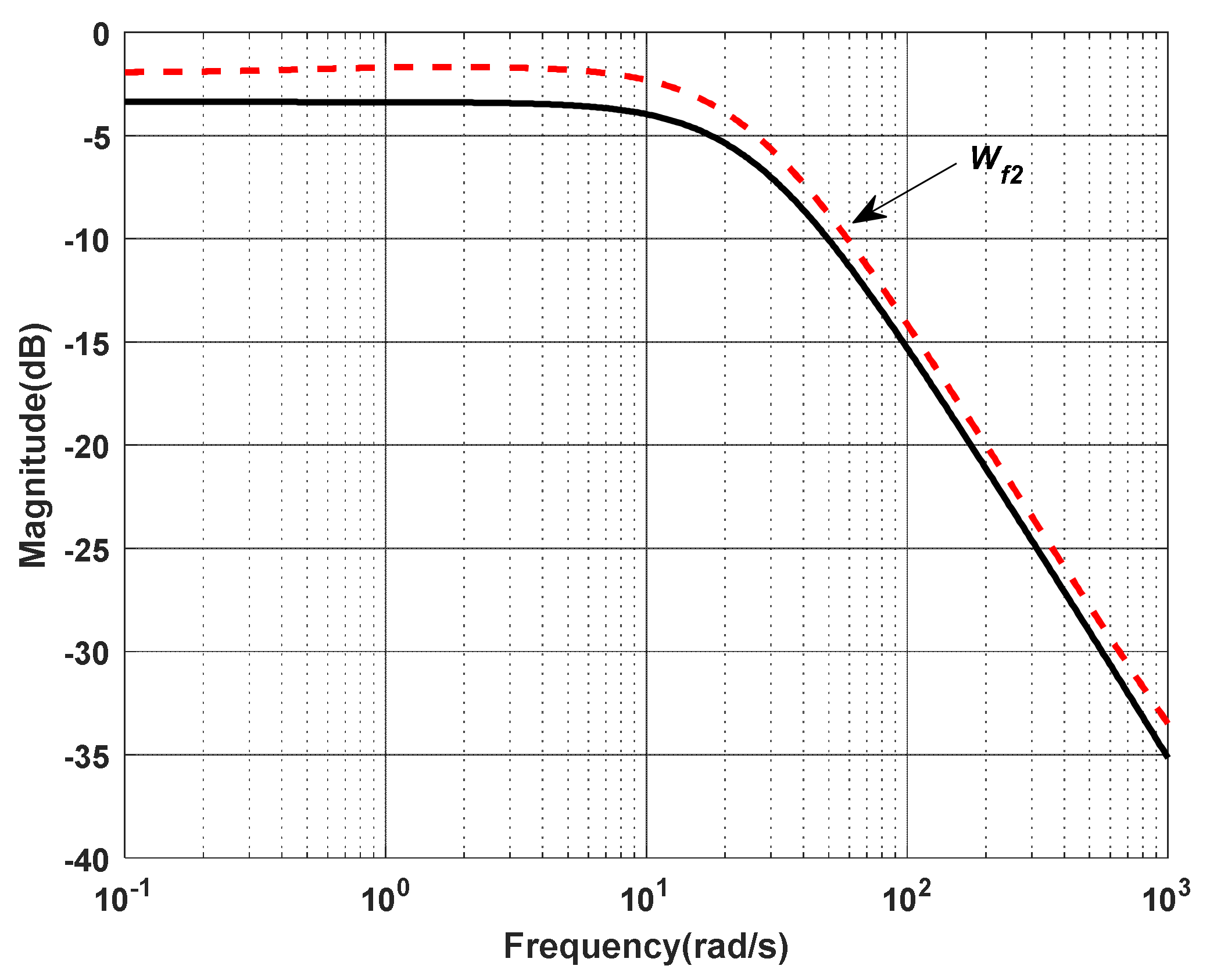
The next step in the design process is to obtain the transfer function $W_{f2}$. The quantity given by Equation (14) for each perturbed plant is constructed, and the uncertainty profile is fitted to the function given by

$$W_{f2}=\frac{0.0065s^2+20.16s+10.08}{s^2+24.85s+12.6}$$

(25)

The uncertainty profile of the perturbed plant transfer functions and the fitted weight function $W_{f2}$ are shown in Figure 9.

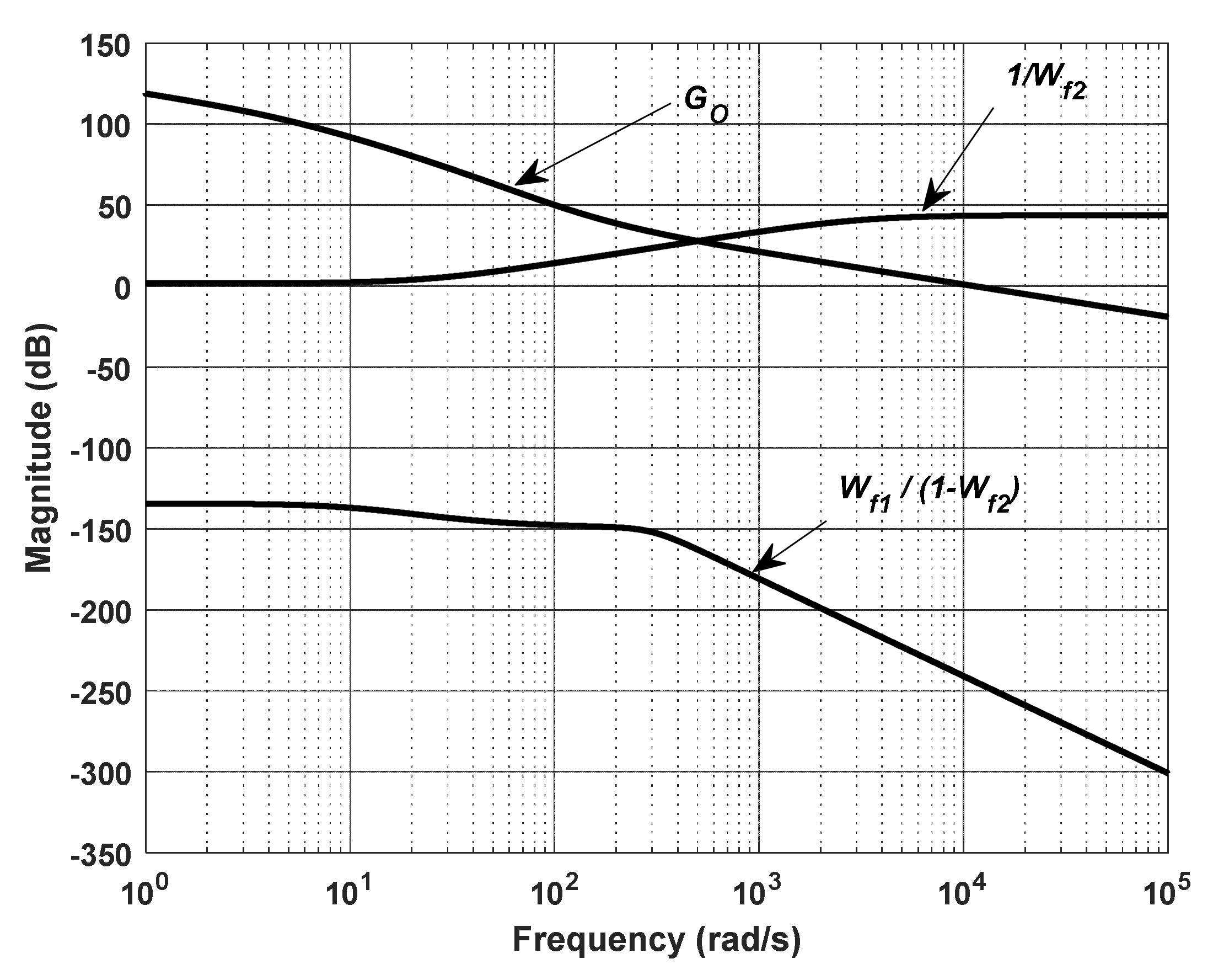
The next step is to construct an open-loop transfer function G_O to satisfy the constraints given in Equations (22) and (23). The open-loop transfer function G_O that satisfies these constraints is fitted to the equation given by

$$G_O=\frac{5.12\times {10}^4\left(s^2+251.9s+12960\right)}{\left(s^3+126s^2+3875s+3750\right)}$$

(26)

Once the open-loop transfer function Go is constructed, the desired robust controller G_C is then obtained from the relationship G_O = G_NG_C and is given by

$$G_C=\frac{1.37\times {10}^3\left(s^2+251.9s+12960\right)\left(s+26.17\right)}{\left(s^3+126s^2+3875s+3750\right)}$$

(27)

A filter transfer function $W_{f1}$ is to be chosen to check for the nominal stability and the robust stability criteria of Equations (20) and (21). A third-order Butterworth filter that fulfills all of the properties for $W_{f1}\left(s\right)$ is chosen as

$$W_{f1}=\frac{K_d{f}_c^2}{s^3+2s^2{f}_c+2s{f}_c^2+f_c^3}$$

(28)

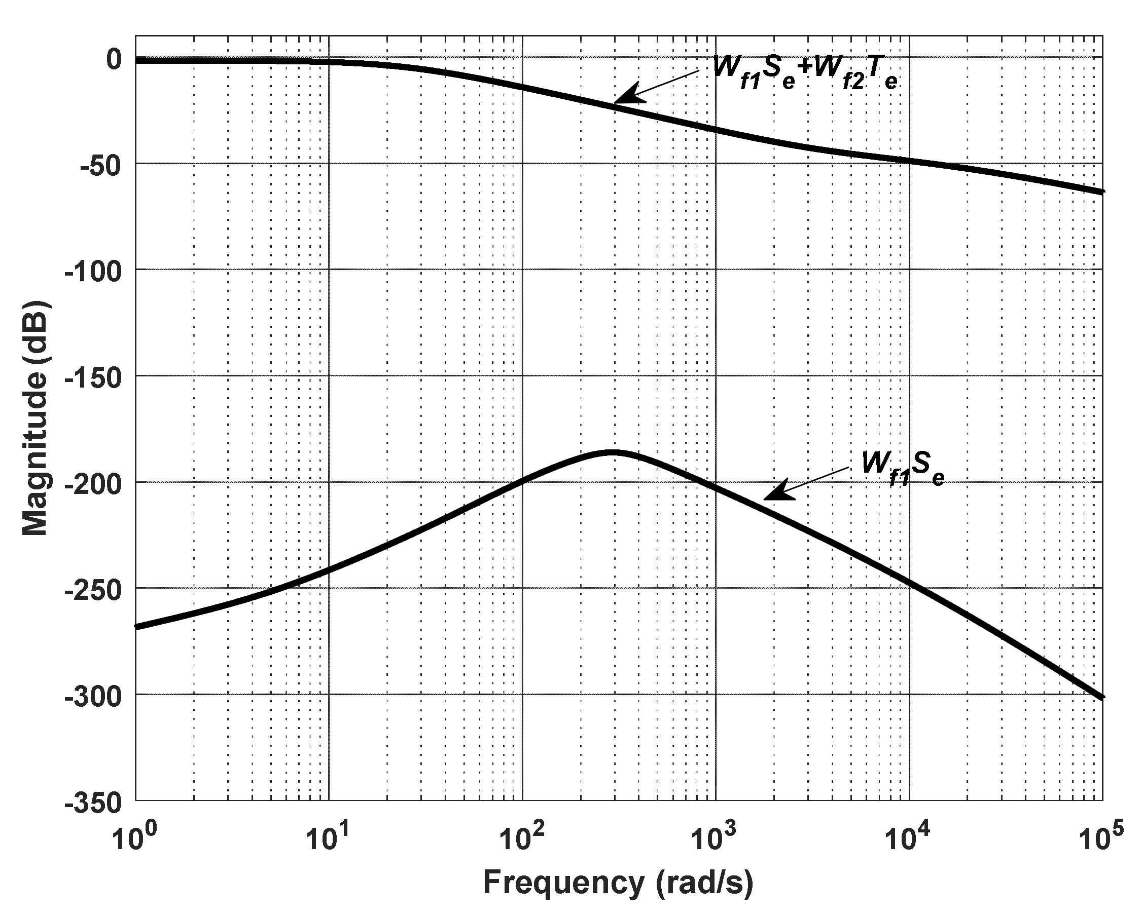
where $K_d={10}^{-5}$ and $f_c=300$. The nominal stability and robust stability criteria of Equations (20) and (21) are to be tested in the next step. The dB-magnitude plots relating $W_{f1}$, $W_{f2}$, and G_O, which were employed to arrive at this controller, are shown in Figure 10. It is evident from Figure 10 that the fitted open-loop function G_O satisfies the bounds set by Equations (22) and (23). The plots for the nominal and robust performance criteria are shown in Figure 11. It is clear from Figure 11 that the condition of (21) is satisfied for all of the frequencies of interest. The nominal performance measure $W_{f1}{S}_e$ is also well satisfied.

The final step in the robust control design using the graphical-loop shaping technique is to verify whether the closed-loop system with the designed robust controller is internally stable or not. This is tested by direct simulation for pre-selected disturbances or inputs.

The performance of the designed robust controller is compared to the classical PI controller tuned using the modulus optimum method. The following section describes a brief tuning method for the conventional PI controller using the modulus optimum method.

3.6. PI Controller Tuning Using the Modulus Optimum Method

The Modulus Optimum (MO) method is a popular technique used to tune the conventional PI control loops for grid-connected VSC [21,22]. A system with one large time constant and many small-time constants can be tuned using the MO method. An Equivalent time constant can be obtained by adding small-time constants. More details on tuning the PI controllers using the MO method for grid-connected VSC are givenin [22,23]. The design steps are briefly described as follows: if the transfer function of a system consists of one large time constant, T_L, and three small-time constants, $T_1,T_2$, and $T_3$, the open-loop transfer function can be given by

$$G_{ol}=\frac{K}{\left(1+T_L\right)\left(1+T_1\right)\left(1+T_2\right)\left(1+T_3\right)}$$

(29)

where $K$ is the system gain. The small-time constants can be added into one equivalent time constant as

$$T_{eq}=T_1+T_2+T_3$$

(30)

Equation (30) can then be written in a simplified form as

$$G_{ol}=\frac{K}{\left(1+T_L\right)\left(1+T_{eq}\right)}$$

(31)

The open-loop transfer function with the conventional PI controller can be given as

$$G_{ol}=K_p\left(\frac{1+s{T}_i}{s{T}_i}\right)\frac{K}{\left(1+T_L\right)\left(1+T_{eq}\right)}$$

(32)

where $K_p$ and $T_i$ are the proportional gain integral and the time constant, respectively. $K_i$ can be obtained from $T_i$ as $K_i=\frac{K_p}{T_i}$.

Using the MO method and upon applying the pole-zero cancellation of the dominating pole of the system and optimizing the absolute value for the closed-loop system with the PI controller to unity, the PI parameters than can be written as

$$K_p=\left(\frac{T_L}{2K{T}_{eq}}\right) and T_i=T_L$$

(33)

The performance of the designed robust controller for the VSC HVDC system is compared to the classical PI controller tuned by the MO method and is tested usingMATLAB/Simulink software in the next section.

4. Simulation of the Designed Robust Controller in MATLAB/Simulink

To verify the performance of the designed robust controller using the graphical loop-shaping algorithm and compare its performance with that of a classical PI controller, simulations were conducted for the switched VSC HVDC system in the SimPowerSystem environment of MATLAB/Simulink. The physical model of the VSC HVDC system is given in Figure 1. To simulate the system under parameter uncertainty, nominal and off-nominal cases were considered in the simulation study. The MATLAB/Simulink model of the VSC HVDC system is shown in Figure 12. For simulation study, it was assumed that 40 MW of real power (i.e., P₁ =P₂ = 40 MW) at unity power factor (i.e., Q₁ = Q₂ = 0 Mvar) was flowing from Grid 1 to Grid 2. The control loops given in Figure 2 and Figure 3 are modeled in MATLAB/Simulink to generate the reference signals for the sine PWM switching algorithm. The switching frequency F_sw used for the sine PWM algorithm was 2850 Hz. The system parameters for the nominal case are given in Table 1, and the classical PI controller parameters, Kp and Ki, obtained using the MO method discussed in Section 3.6, were found to be Kp = 25.3650 and Ki = 190. The transfer function for the robust loop shaping controller is given by Equation (27).

For the simulation study, a real power of 40 MW (i.e., P₁ = P₂ = 40 MW) at unity power factor (i.e., Q₁ = Q₂ = 0 Mvar) flowing from Grid-1 to Grid-2 is commanded. A comparison of the results between the robust controller and conventional PI controller tuned using the modulus optimum methods is shown in Figure 13, Figure 14, Figure 15 and Figure 16. The nominal system parameters used in the study are shown in Table 1. Under these conditions, the system is considered to be running under nominal conditions (nominal case). When one of the lines is taken out for maintenance for both the converter stations, this system condition is considered as an off-nominal case. In this case, the total system resistance (R) and the total system inductance (L) change. 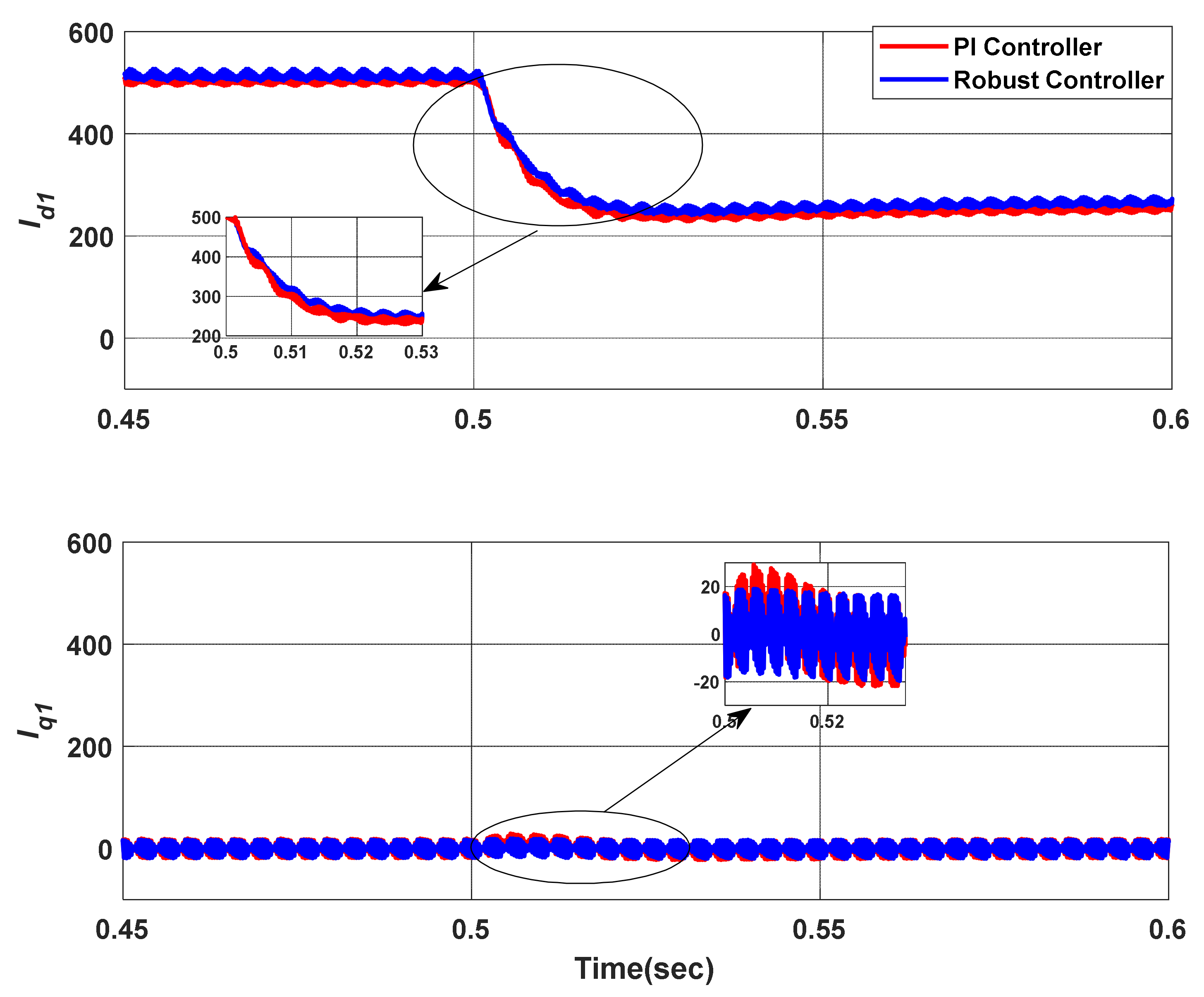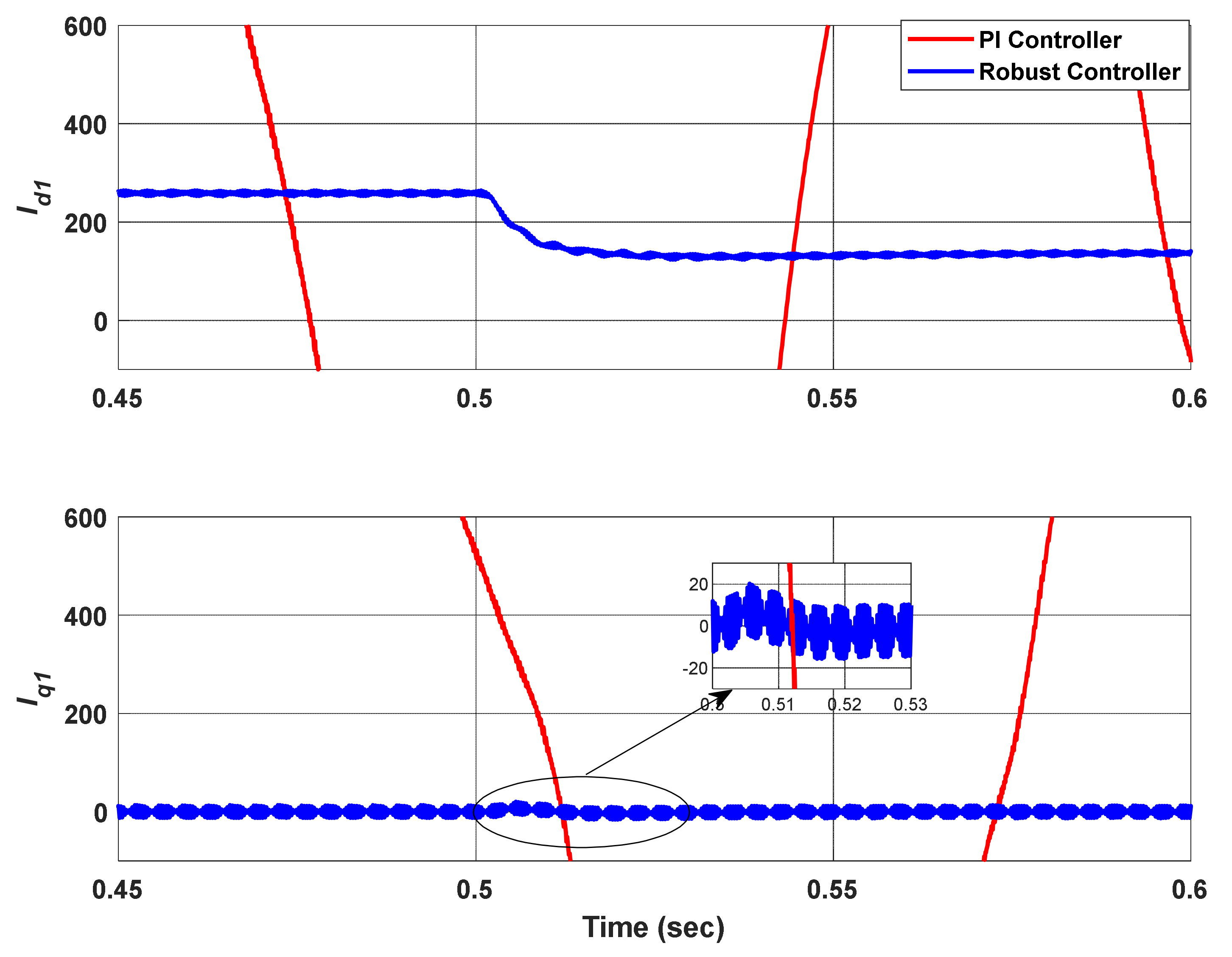The change in the the value of L is reflected in the decoupled control loop of Figure 2 and Figure 3 by switching to the new value of L in the decoupled loop. The d-q current response I_d1 and I_q1 for the nominal and the off-nominal cases for a 50% step change in the active power is shown in Figure 13 and Figure 14, respectively. 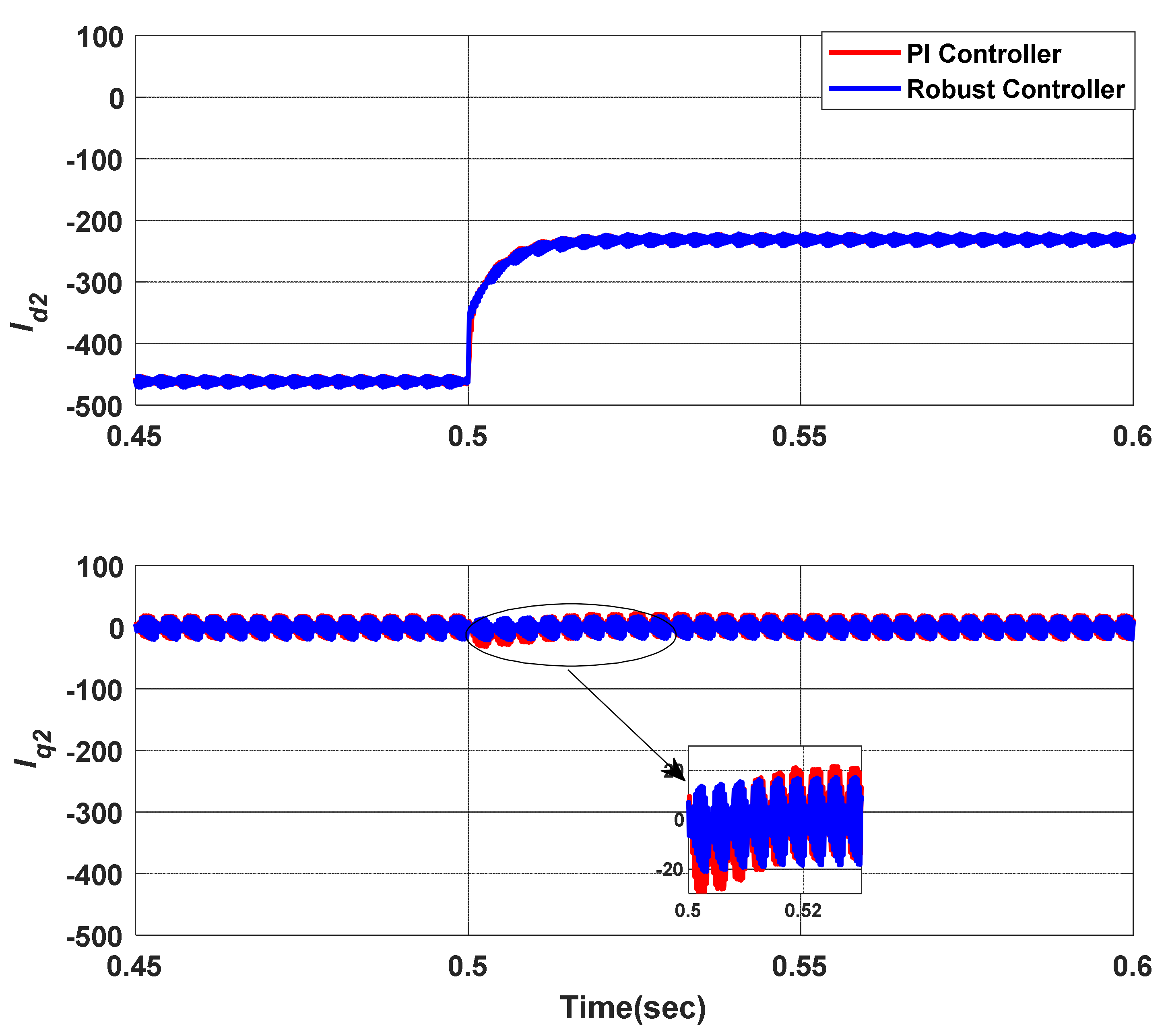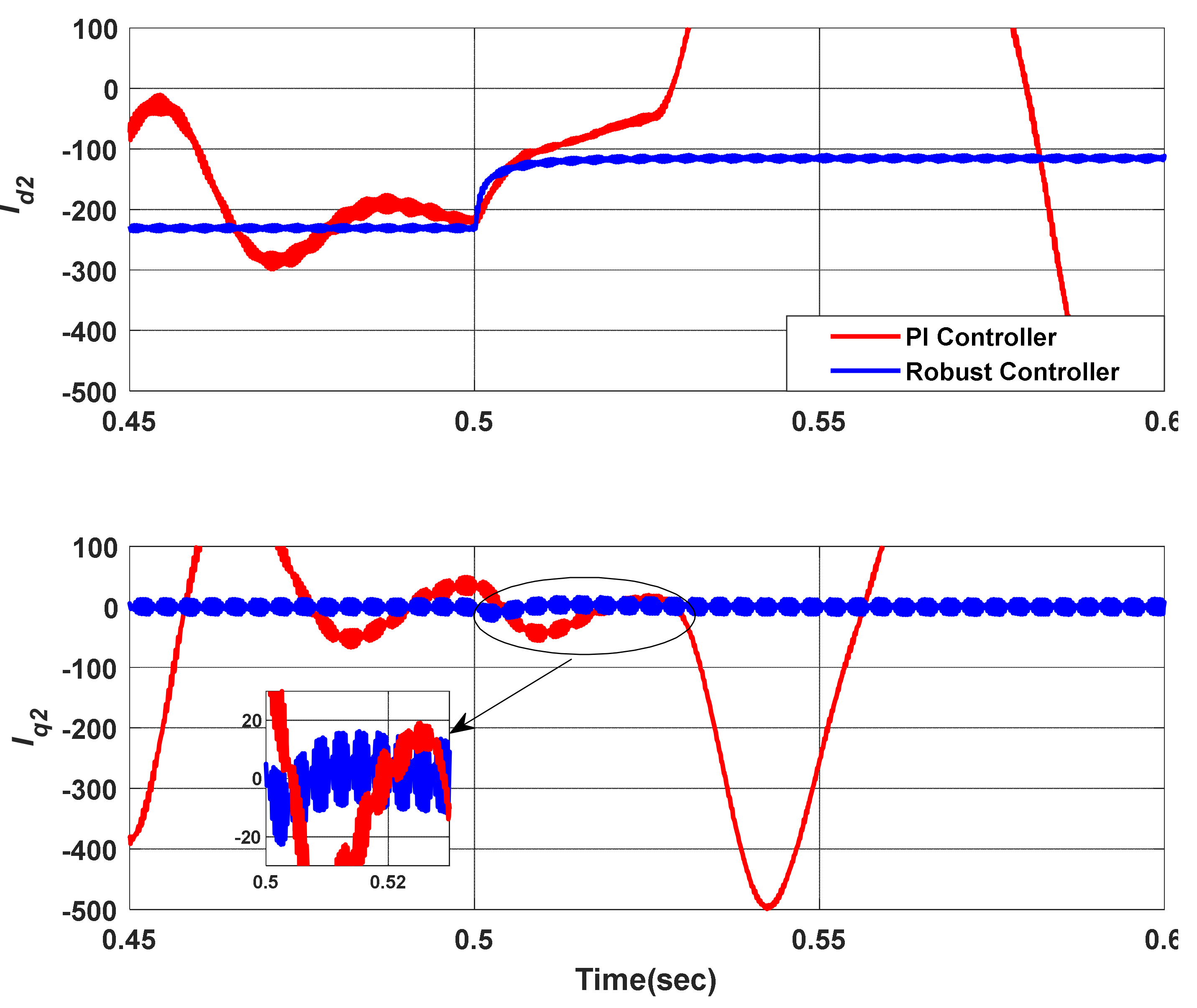Figure 15 and Figure 16 demonstrate the response of currents I_d2 and I_q2 for the nominal and off-nominal case when the system is subjected to a 50% step change in active power. It is clear from the responses that the robust controller and the traditional PI controller give an identical performance for the nominal case but that the PI controller gives an unstable response for the off-nominal case. The response of the classical PI controller for the off-nominal case is degraded because the variations in the system parameters change the open-loop transfer function of the VSC HVDC system, and the tuned Kp and Ki values are no longer valid for the off-nominal case.

The designed robust loop-shaping controller gives superior performance even for the off-nominal case. This is expected as the traditional PI controller is tuned to give the best performance at the nominal case, but for the proposed robust controller, the variations in the system uncertainties are considered during the design steps.

Since the perturbations only affect the inner loop variables and the designed robust controller can stabilize the inner loop, the outer loop is tuned using the classical PI controller. The simulation results show that the designed robust loop-shaping controller shows excellent performance for both nominal and off-nominal cases.

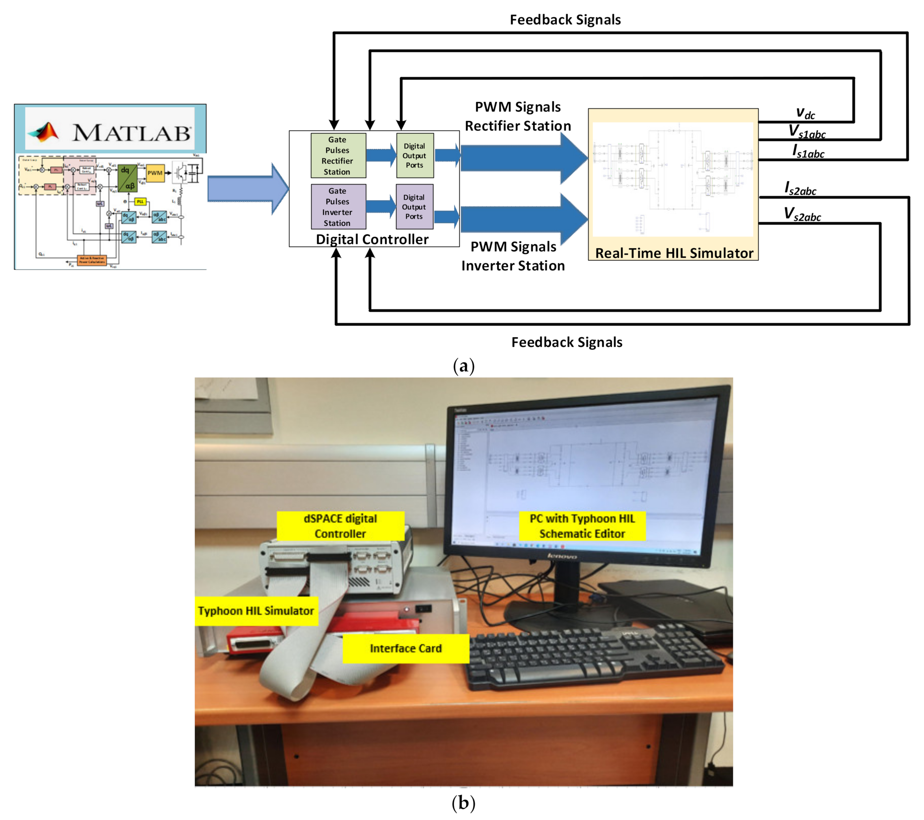
5. Experimental Validation of Robust Controller

The performance of the designed robust loop-shaping controller is also verified experimentally. The robust controller designed through the graphical loop-shaping technique in Section 3 is implemented in the lab on a dSPACE digital controller on the MATLAB/Simulink platform. A Typhoon real-time hardware in the loop (HIL) 604 simulator was used to build the model of the VSC HVDC system shown in Figure 1. The nominal system parameters used for the real-time simulation are given in Table 1, and the robust controller transfer function is given by Equation (27). The presence of hardware in the real-time simulation process helps in the proper prediction of the behavior of the control system before the implementation on the actual system [24]. The schematic and the picture of the experimental implementation of the designed robust controller in the lab are shown in Figure 17. In this setup, the VSC HVDC system is modeled in the Typhoon schematic editor. A very small simulation Step of 2 µsec is used to guarantee the behavior of the modeled system close to the actual VSC HVDC system. The designed robust loop-shaping controller and the control loops of Figure 2 and Figure 3 are programmed in MATLAB/Simulink environment, and the control scheme is implemented on a dSPACE-based digital controller, a MicroLabBox (Control Desk 7.3, 2020, dSpace GmbH, Paderborn, Germany) with 25 µsec sampling time. The actual feedback signals are input into the controllers as shown in Figure 16. The experimental results are shown in Figure 18, Figure 19, Figure 20 and Figure 21.

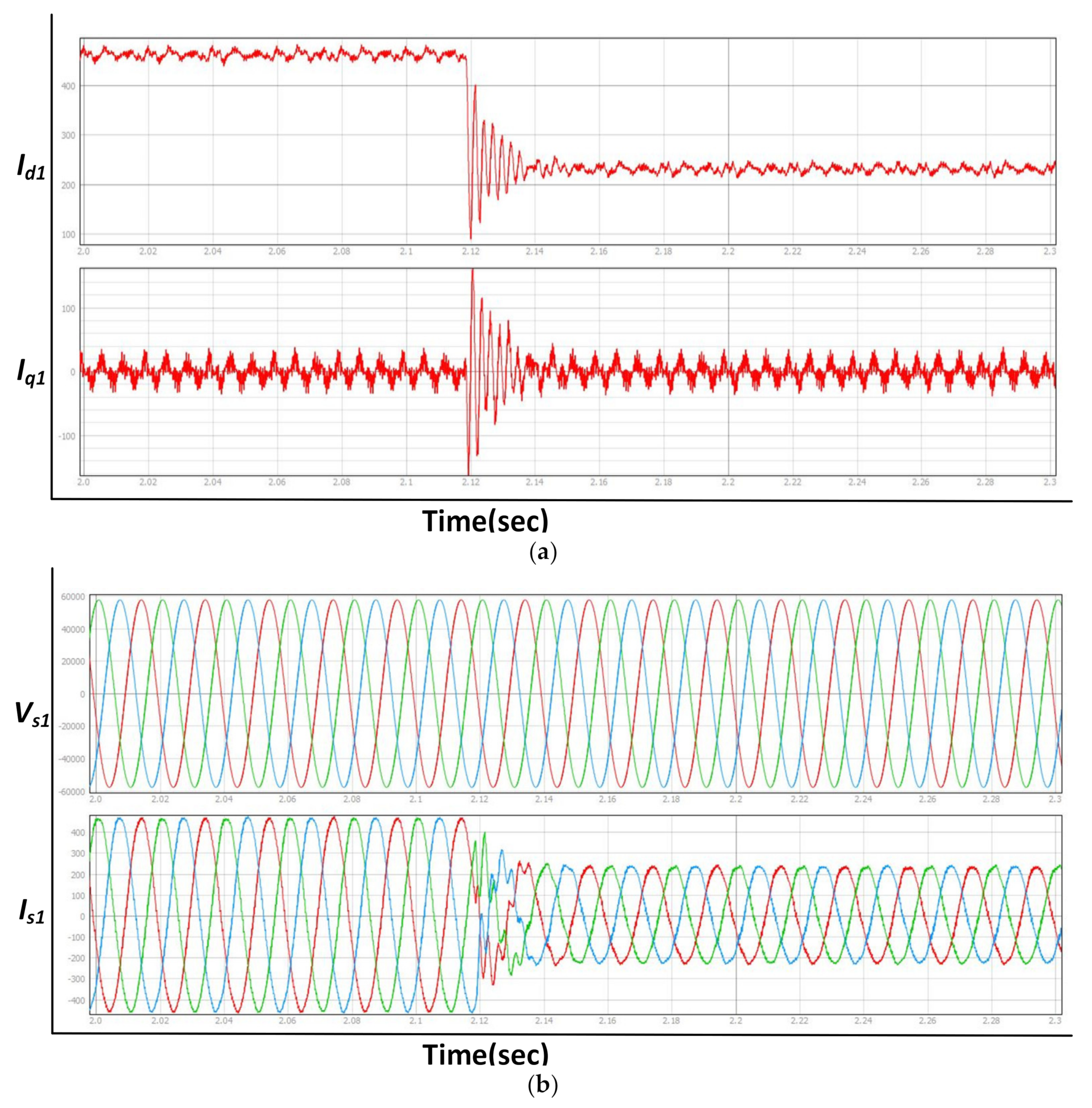
The d-q currents, I_d1, I_q1, and the grid voltage and current V_s1 (three phase votlages) and I_s1 (three line currents) for the Converter Station 1 for a 50% step change in active power at t = 2.18 s. are shown in Figure 18. It is clear from Figure 18a that the d-q currents reach the steady-state within 18 ms. Additionally, as it can be seen from Figure 18b, the grid current stabilizes within two cycles.

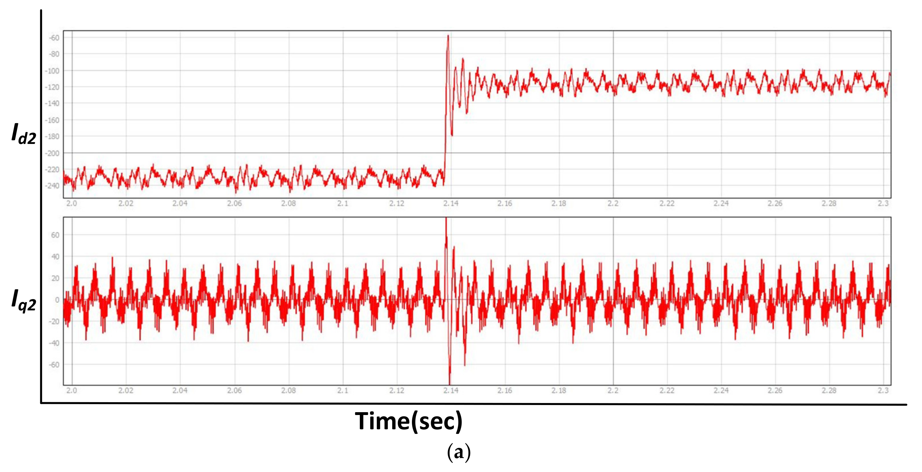
Figure 19 shows the experimental results for the off-nominal case (when one of the transmission lines is taken out for maintenance) for a step change in active power at t = 2.056 sec. It is evident from Figure 19a that the d-q currents I_d1 and I_q1 are stable even in this worst-case scenario and that the designed robust controller can achieve the d-q quantities of the Conv-1 to steady-state value very fast, within 8 m sec. The grid voltage, V_s1, and the grid current I_s1 for the off-nominal case for Conv-1 are shown in Figure 19b, and as evident from Figure 19b, which also shows thatthe grid current reaches steady within 1.5 cycles. The grid integrity is maintained by the robust controller for the off-nominal case as well.

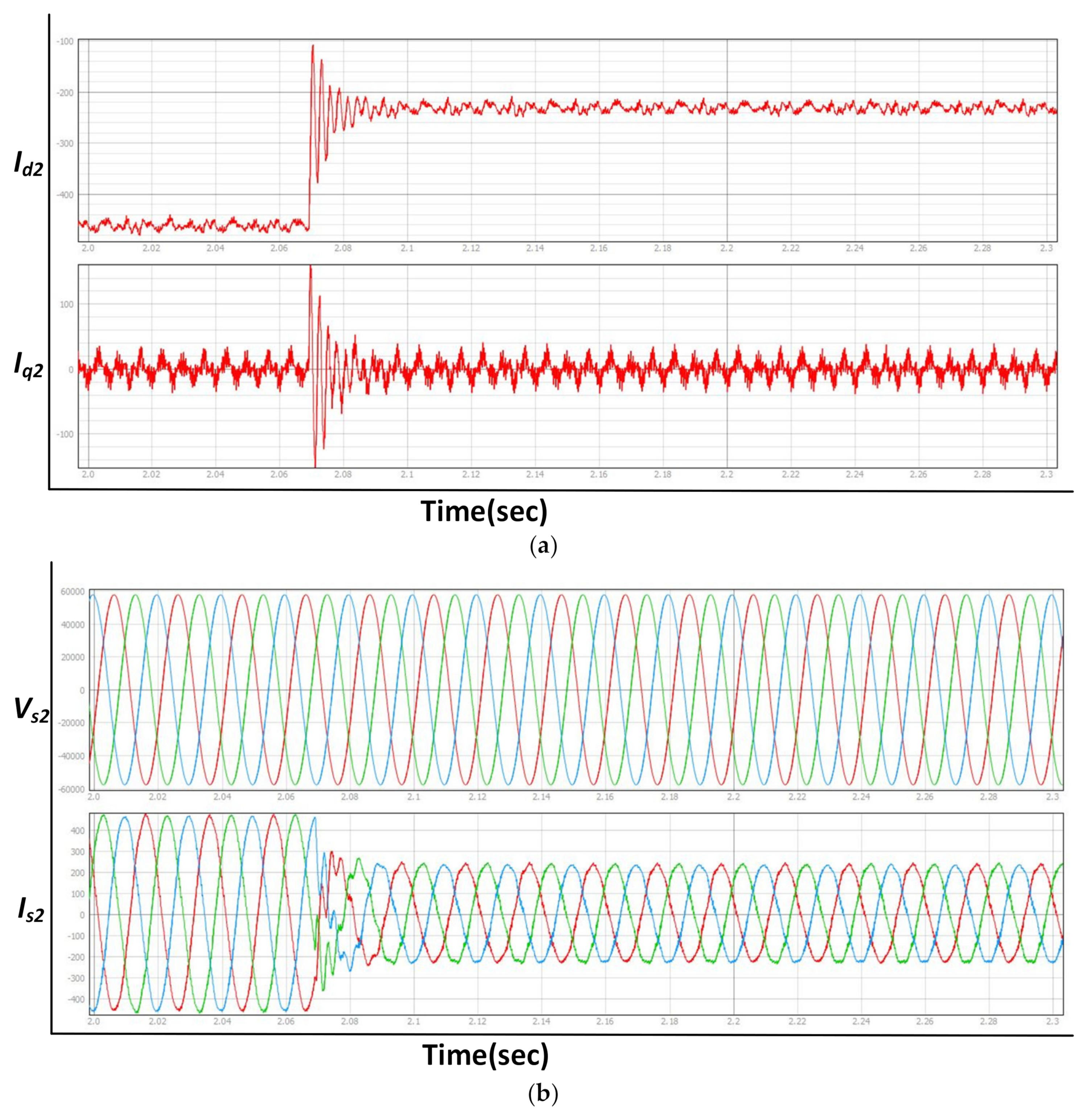
The experimental results for the Conv-2 for the nominal case are shown in Figure 20. The considered distburbance is a 50% step change in the active power at t = 2.07 sec. Figure 20a shows the d-q currents I_d2 and I_q2. The robust controller that was designed using the loop-shaping algorithm demonstrates a fast response, and the system stabilizes within 18ms. The grid current response for the nominal case is shown in Figure 20b. The transients in the grid current I_s2 reach the steady-state value within 2 cycles.

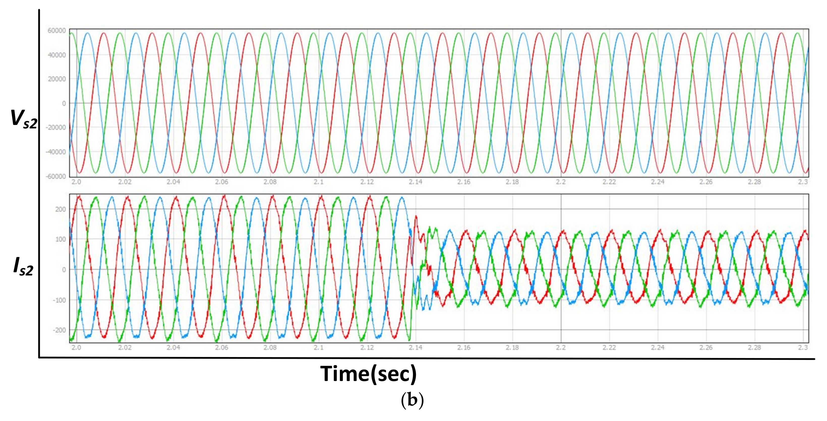
The response for the off-nominal case for Conv-2 is shown in Figure 21. The experimental results demonstrate the effectiveness of the designed robust loop-shaping controller in stabilizing the system not only for the nominal case but also for the off-nominal case.

6. Conclusions

A robust controller for the internal d-q current loops of a VSC HVDC system has been designed through a graphical loop-shaping procedure. Unlike the H∞ approach, the graphical loop-shaping used in this paper is a simple technique avoiding complex minimization procedures. In the loop-shaping method, uncertainty is addressed indirectly using the perturbed plant transfer functions. The shaped plants are chosen based on the graphical loop-shaping concept, wherein both the necessary as well as the sufficient conditions of the robust performance are applied. This method is more intuitive for the designer, as the controller can be directly extracted from the open-loop transfer function of the shaped plant. The design yields a fixed parameter controller making its implementation straightforward. The designed controller is tested both using simulations in MATLAB and also experimentally verified using a real-time simulator. Simulation and experimental results show that the proposed robust controller not only achieves good performance under nominal cases but also achieves superior performance under plant perturbations considered during the design procedure. Extending this work for other systems such as grid-connected renewable systems, variable speed AC drives, and electric vehicles to include uncertainty in the switching frequency and grid parameter uncertainty will be interesting work for the future.