
Generation Data of Synthetic High Frequency Solar Irradiance for Data-Driven Decision-Making in Electrical Distribution Grids


Abstract
:1. Introduction
- In contrast to recorded measurement data and to approaches used in commercial software [7], a model is more general and non-biased against the occurrence of a specific scenario.
- For stochastic numerical simulation, an infinite amount of data can be generated.
- To investigate the sensitivity of a numerical simulation to specific model parameters, we can change the parameters of the model.
1.1. Literature Review
1.2. Contribution
- We provide a comprehensive model of PV systems power production that is suitable for the numerical simulation of electrical distribution grids.
- The dependency of temporal weather variations, including one-minute, daily, and monthly variations on the PV systems power production, is considered. A model is developed to generate a sequence of PV systems power production with a random average based on the N-state MC model of that day.
- A distinct N-state MC model is proposed for each group of days characterized by cloudy, intermittent cloudy, and clear sky. The proposed model is tested on two locations with ‘‘warm and temperate” and ‘‘tropical wet and dry/savanna” climates.
1.3. Organization
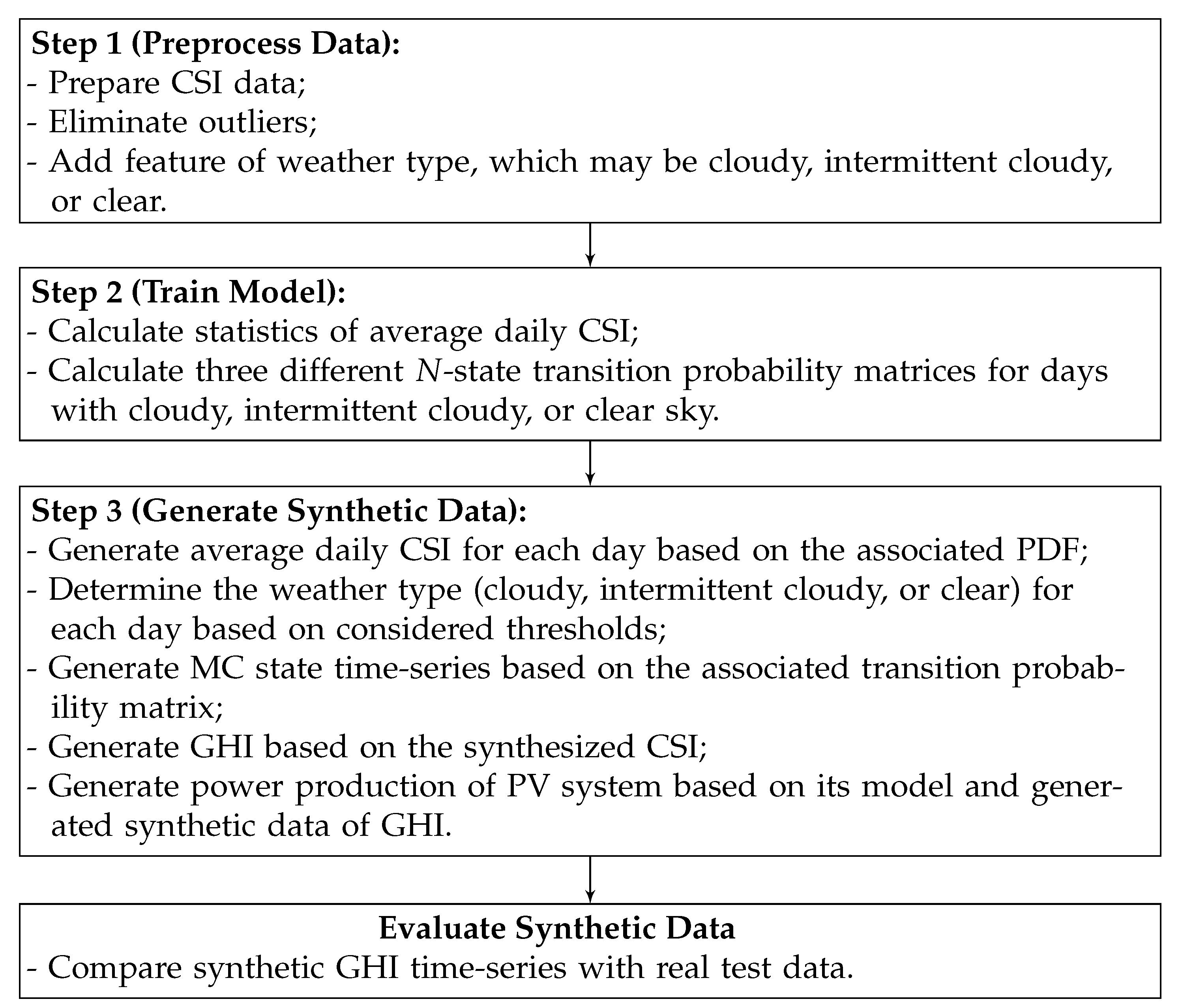
2. Proposed Model
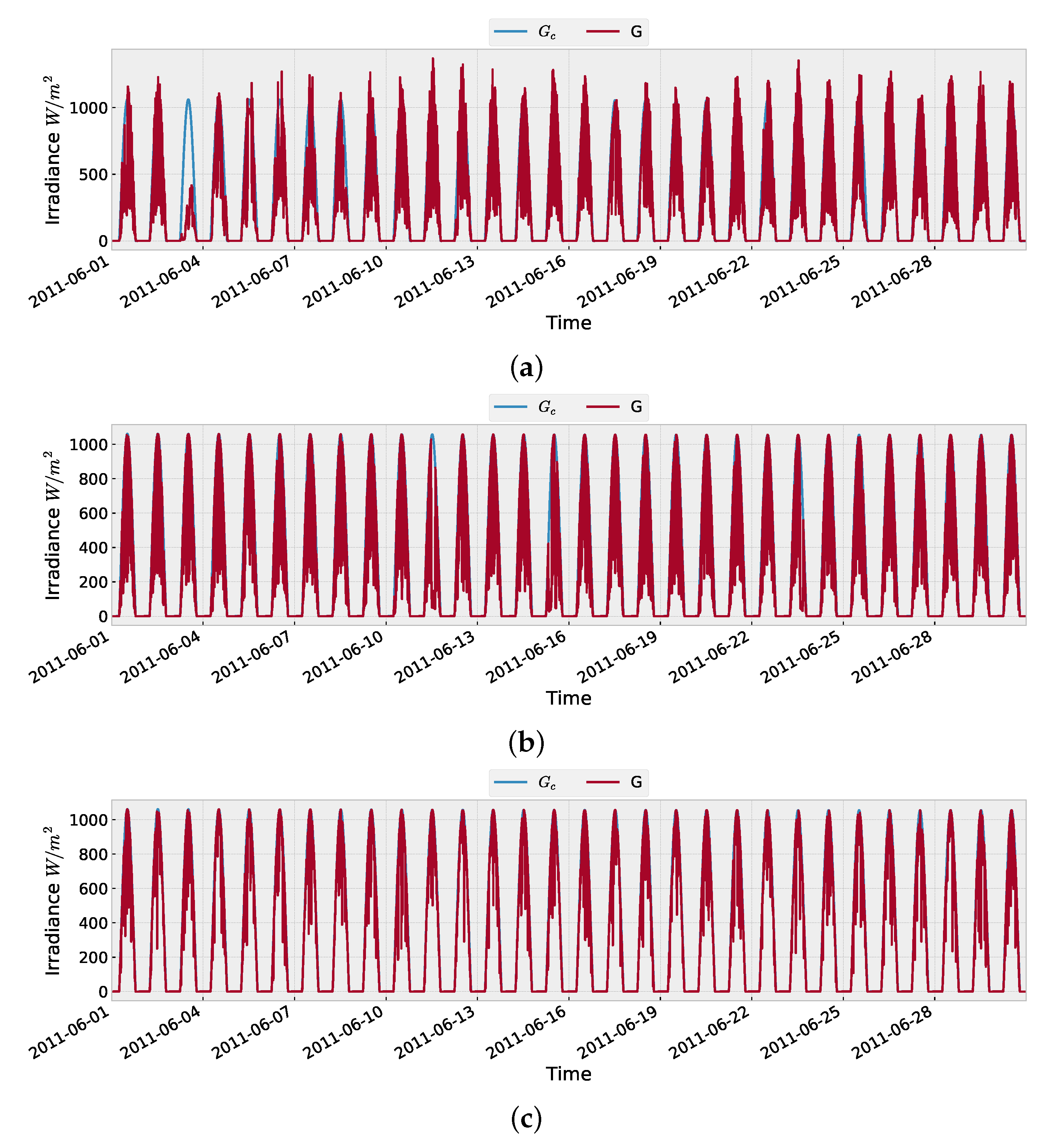
2.1. Step 1 (Preprocess Data)
2.2. Step 2 (Train Model)
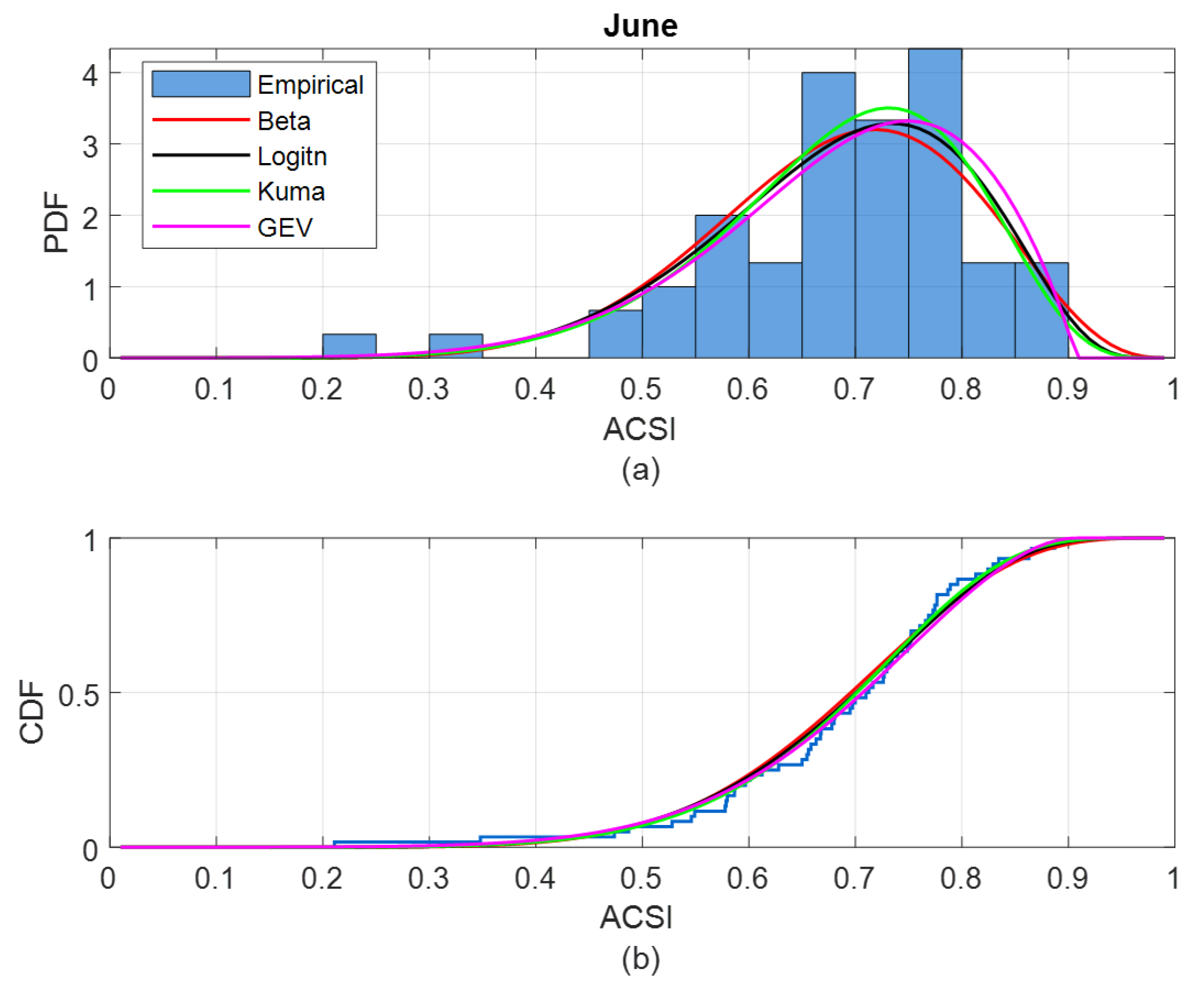
2.2.1. Pool of Selected Probability Density Functions
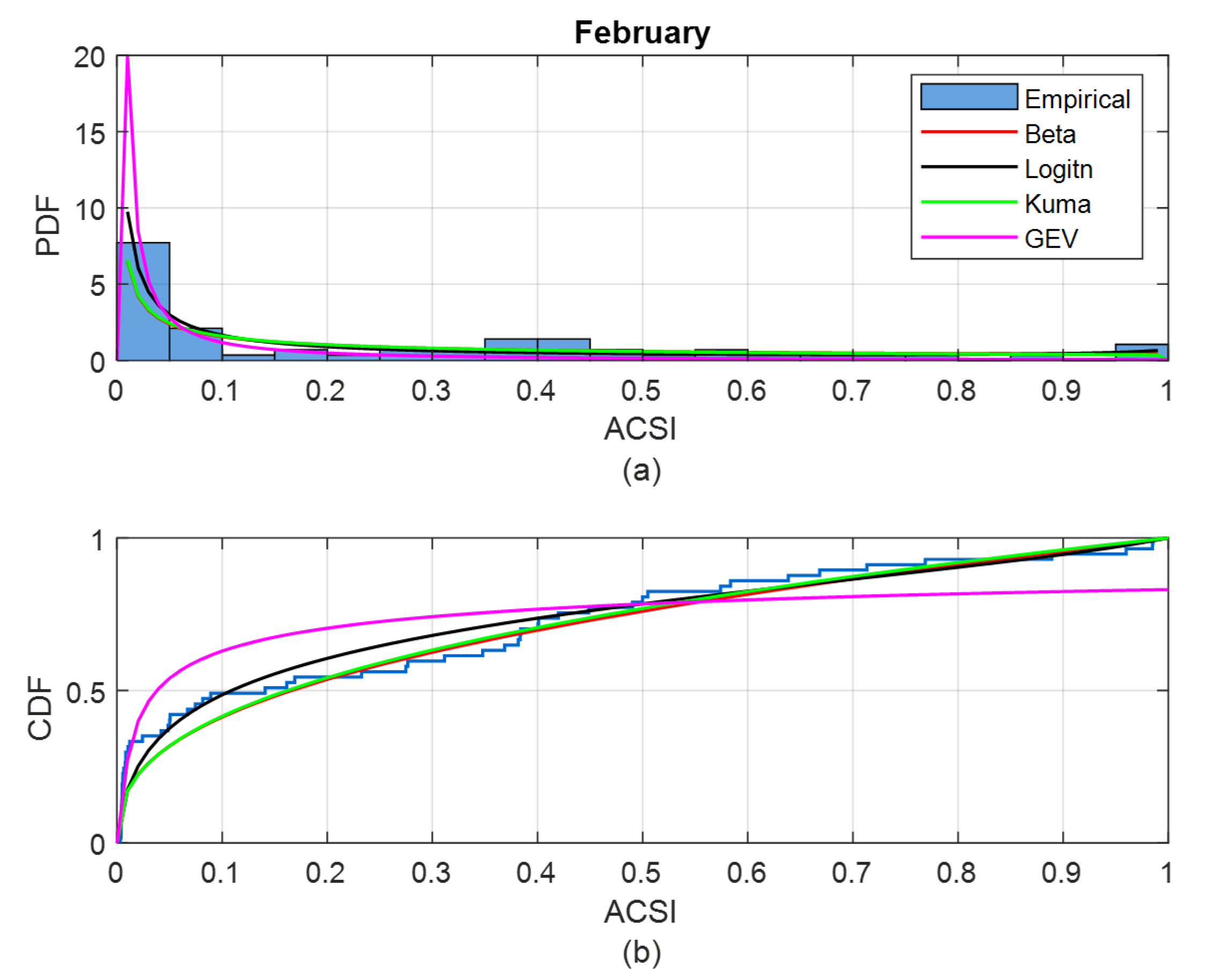
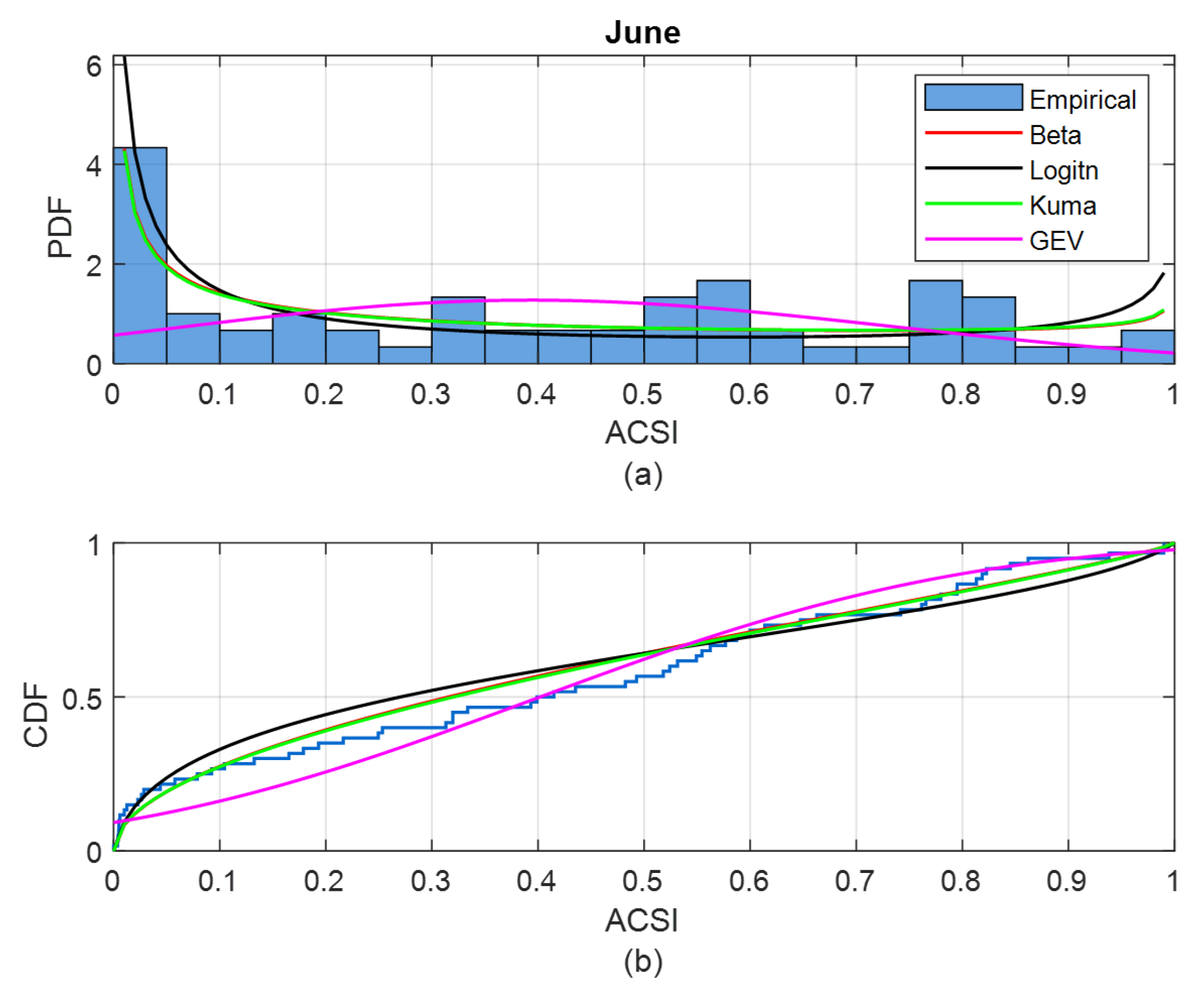
2.2.2. Parameter Estimation of Probability Density Function and Goodness of Fitting Test
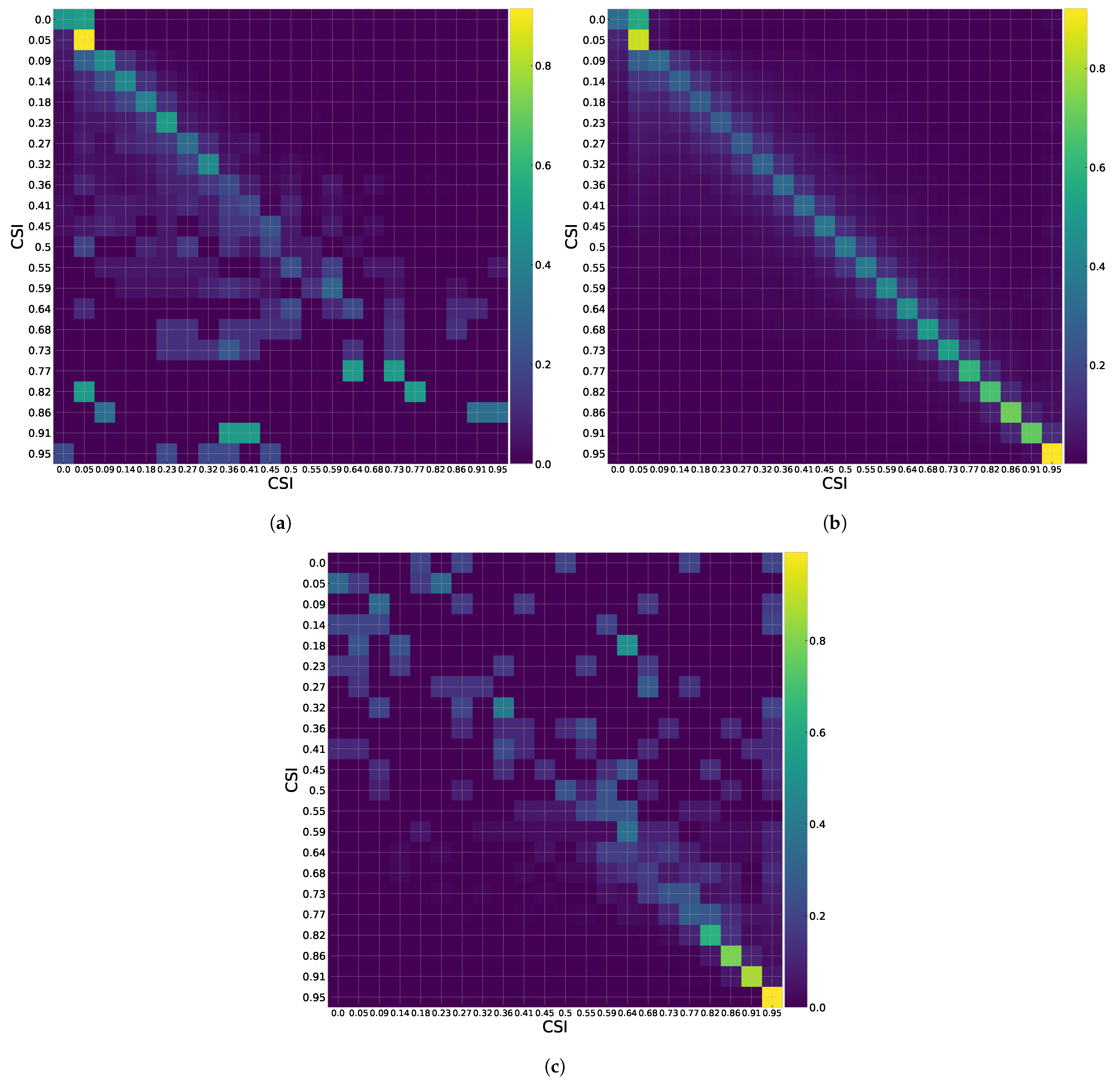
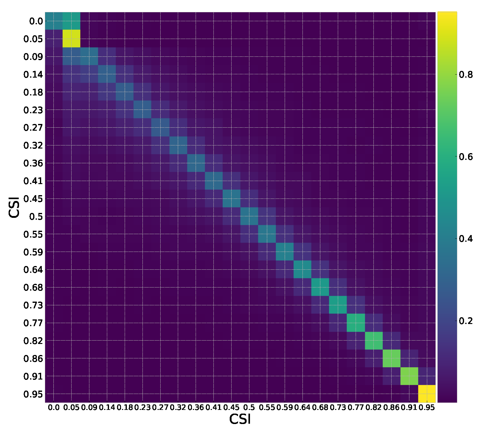
2.2.3. Markov Chain Training
2.3. Step 3 (Generate Synthetic Data)
2.4. Evaluate Synthetic Data
- similarity of PDFs in different months to evaluate the impacts of monthly weather variation on GHI;
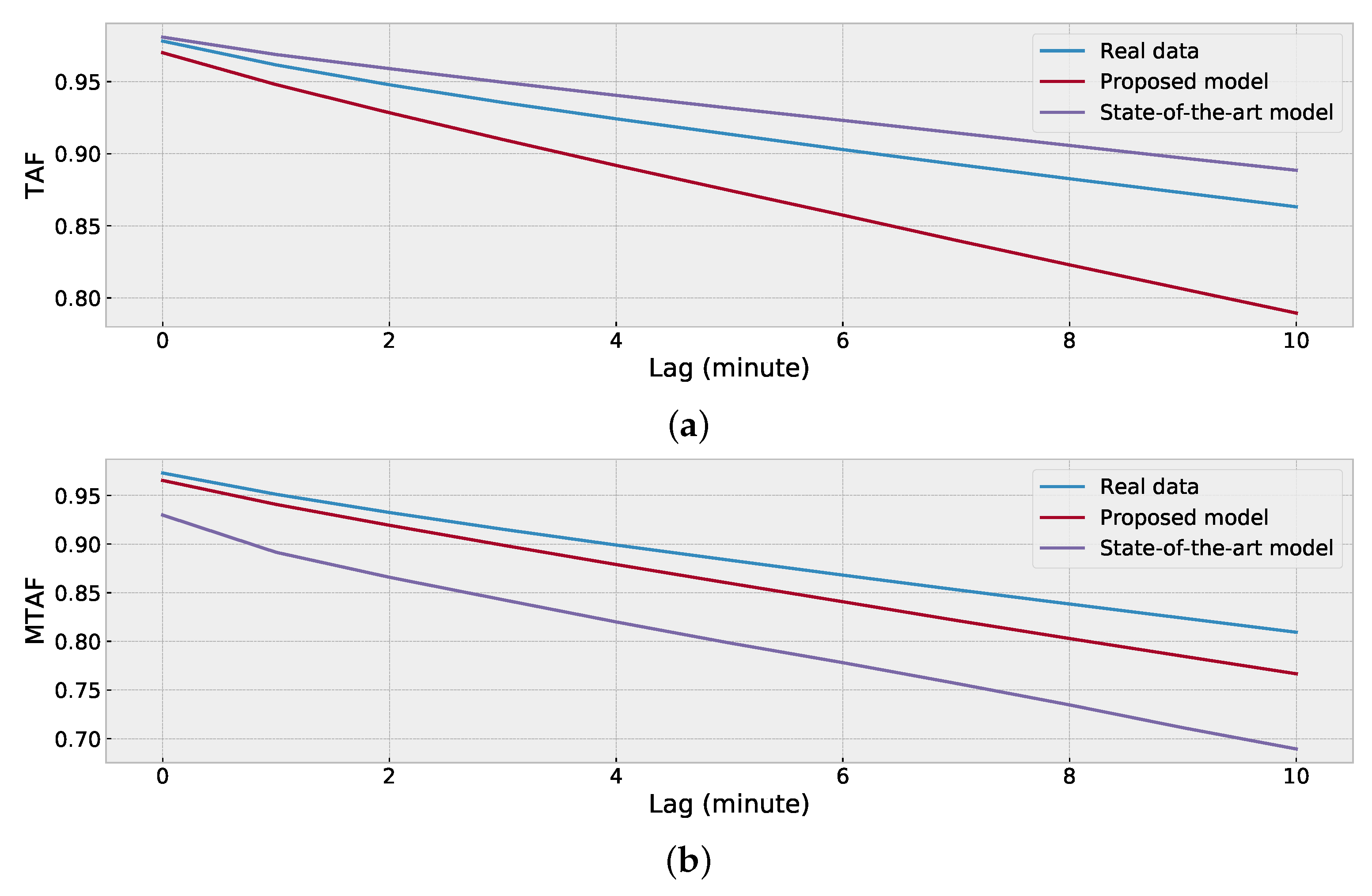
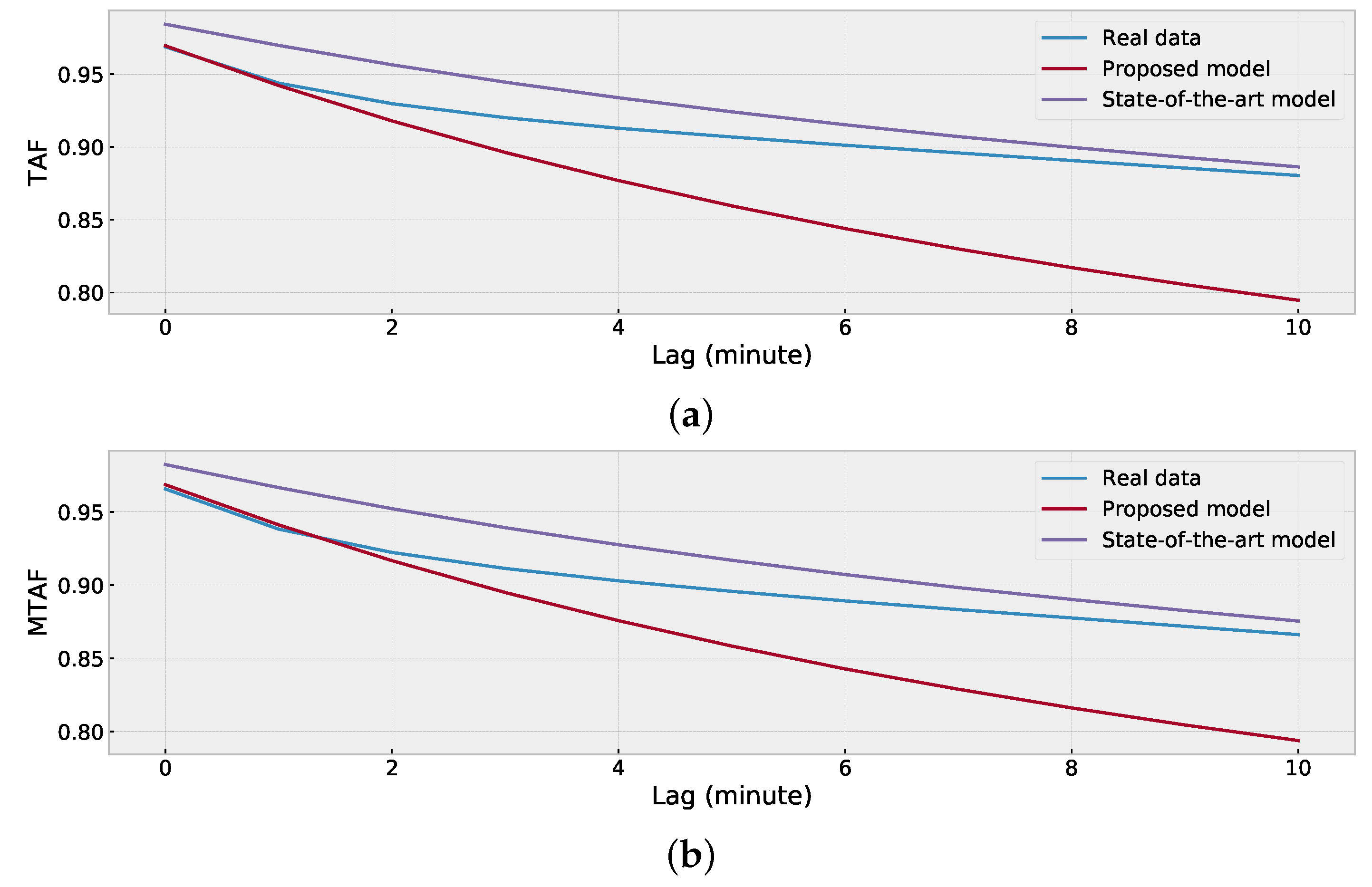
- TAF similarity of average daily GHI for evaluating the impacts of daily weather variation on GHI; and
- TAF similarity of GHI time-series for evaluating the impacts of one-minute-resolution weather variations.
2.5. Benchmark Model
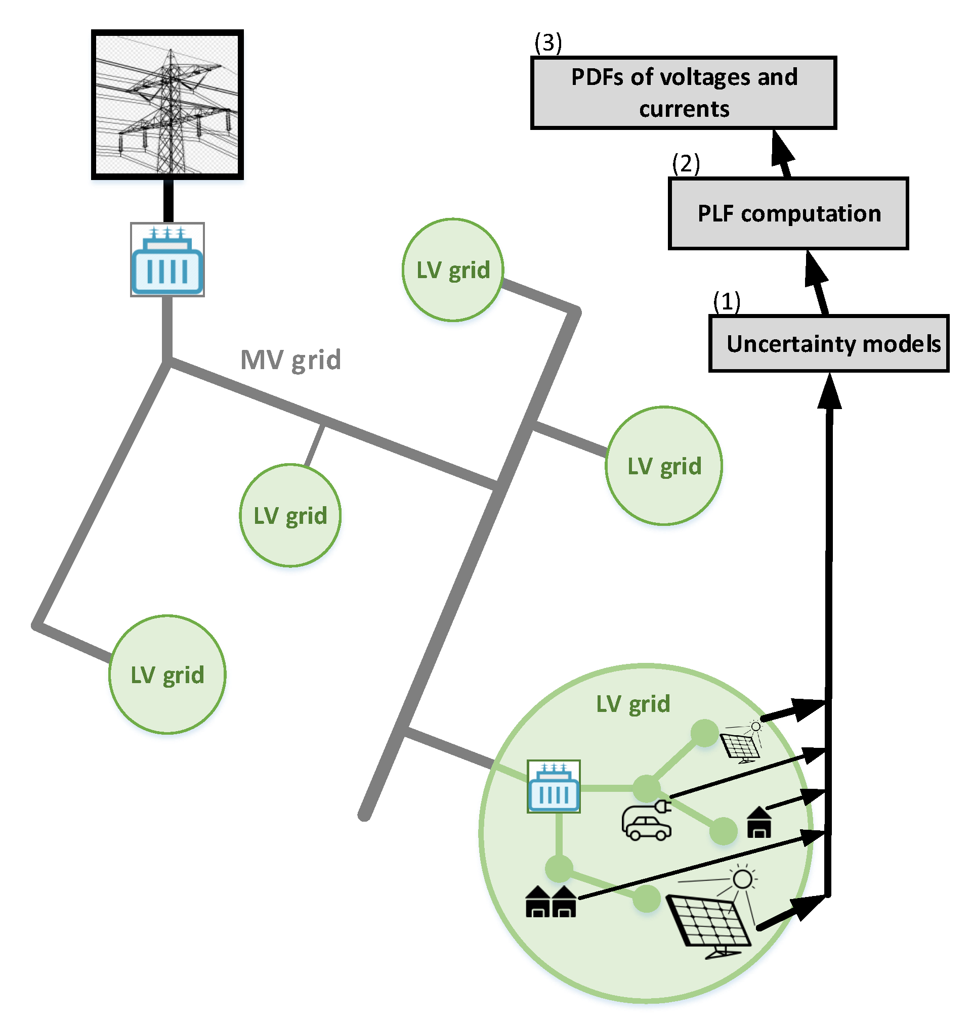
3. Exemplary Applications of the Proposed Model
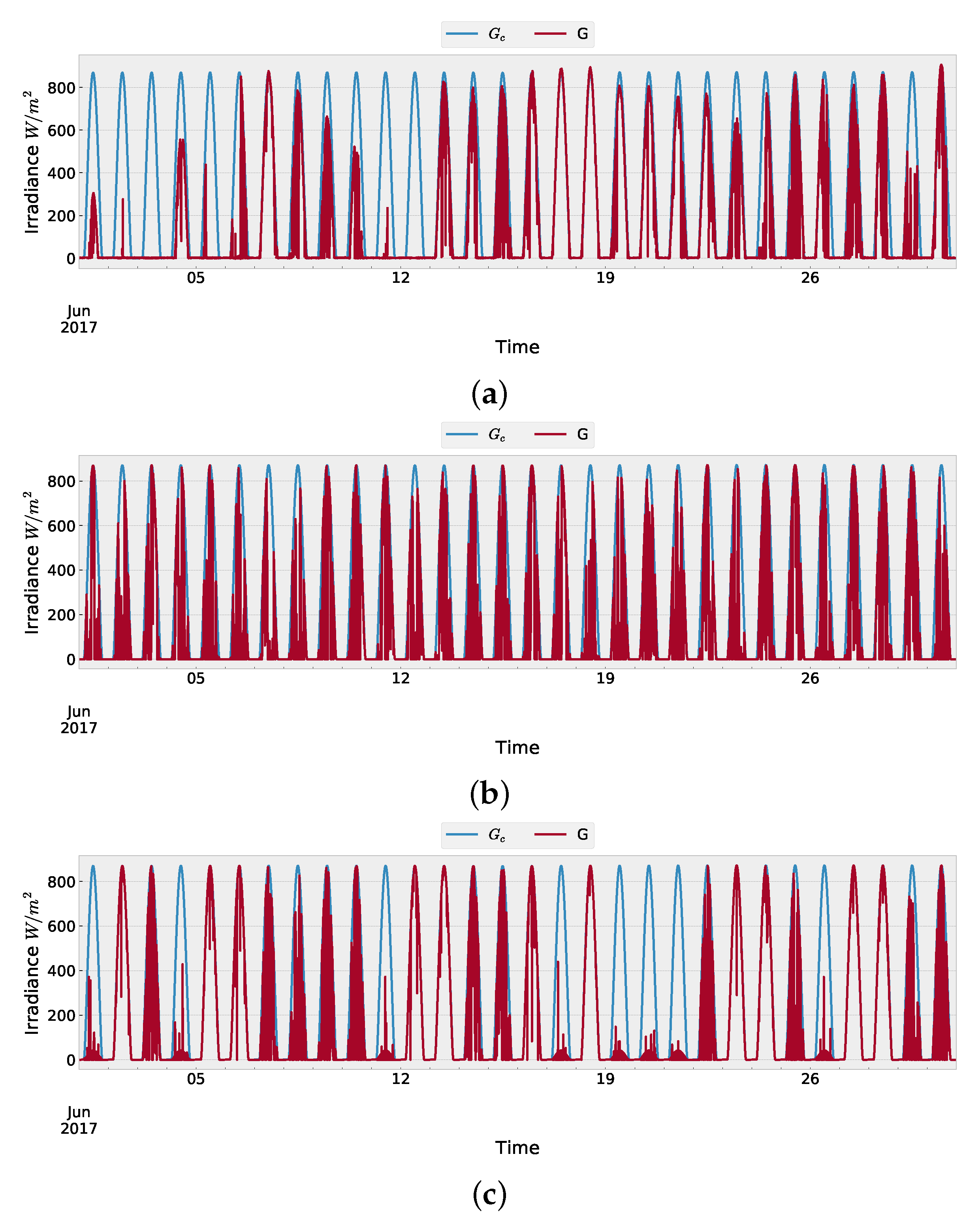
4. Experimental Results
4.1. Input Data
4.2. Model Training on Data of Location (a)
4.3. Synthetic Data Generation at Location (a)
4.4. Evaluation of Synthetic Data of Location (a)
4.5. Model Training on Data of Location (b)
5. Conclusions and Future Works
Author Contributions
Funding
Institutional Review Board Statement
Informed Consent Statement
Data Availability Statement
Conflicts of Interest
Abbreviations
| BSRN | Baseline Surface Radiation Network |
| COP21 | 21st Conference of Parties |
| CSI | Clear Sky Index |
| DC | Determination Coefficient |
| EV | Electric Vehicle |
| GEV | Generalized Extreme Value |
| GHI | Global Horizontal Irradiance |
| GoF | Goodness of Fitting |
| HMM | Hidden Markov Model |
| Kuma | Kumaraswamy |
| LogitN | Logit-Normal |
| Logist | Logistic |
| Log-Log | Log-Logistic |
| LV | Low-Voltage |
| MC | Markov Chain |
| MLE | Maximum Likelihood Estimation |
| MTAF | Modified Temporal Autocorrelation Function |
| MV | Medium-Voltage |
| Probability Density Function | |
| PLF | Probabilistic Load Flow |
| PV | Photovoltaic |
| SCSI | State of Clear Sky Index |
| SFOE | Swiss Federal Office of Energy |
| TAF | Temporal Autocorrelation Function |
| WRMC | World Radiation Monitoring Center |
Nomenclature
| Indices | |
| m | Month |
| d | Day |
| t | Minute time-step |
| Lag of TAF in minutes | |
| Functions | |
| Beta PDF | |
| Kumaraswamy PDF | |
| Logit-Normal PDF | |
| Logist PDF | |
| Log-Log PDF | |
| GEV PDF | |
| Standard TAF | |
| Modified version of TAF | |
| Variables | |
| Measured GHI at month m, day d, and time step t | |
| Synthetic GHI at month m, day d, and time step t | |
| Clear sky GHI at month m, day d, and time step t | |
| Clear Sky Index at month m, day d, and time step t | |
| State of CSI at month m, day d, and time step t | |
| , | Minimum and maximum of tolerance band |
| , | 0.25 and 0.75 quantile of the measured GHI |
| Type of day d of month m | |
| Average of CSI over day d at month m | |
| Standard deviation of CSI over day d at month m | |
| Residual of CSI average from the centers of clusters | |
| Residual of CSI standard deviation from the centers of clusters | |
| Transition matrix of a day type | |
| Parameters | |
| Number of days in month m | |
| , | Average thresholds to cluster the days |
| , | Standard deviation thresholds to cluster the days |
| a, b | Shape parameters of Beta PDF |
| c, d | Shape parameters of Kumaraswamy PDF |
| , | Average and standard deviation of of Logit-N PDF |
| , s | Average and scale parameter of of Logist PDF |
| , v | Log average and log scale parameter of Log-Log PDF |
References
- Rhodes, C.J. The 2015 Paris climate change conference: COP21. Sci. Prog. 2016, 99, 97–104. [Google Scholar] [CrossRef]
- SFOE. Potenzialabschätzung für Sonnenkollektoren im Wohngebäudepark; Swiss Federal Office of Energy: Bern, Switzerland, 2018. [Google Scholar]
- Hänni, J. Energy Transition in Switzerland. In Energy Law and Economics; Springer: Berlin/Heidelberg, Germany, 2018; pp. 43–57. [Google Scholar]
- Ramadhani, U.H.; Shepero, M.; Munkhammar, J.; Widén, J.; Etherden, N. Review of probabilistic load flow approaches for power distribution systems with PV generation and electric vehicle charging. Int. J. Electr. Power Energy Syst. 2020, 120, 106003. [Google Scholar] [CrossRef]
- Bahaidarah, H.M.; Tanweer, B.; Gandhidasan, P.; Rehman, S. A combined optical, thermal and electrical performance study of a V-trough PV system—Experimental and analytical investigations. Energies 2015, 8, 2803–2827. [Google Scholar] [CrossRef] [Green Version]
- Gunal, M.M. Simulation for Industry 4.0; Springer: Berlin/Heidelberg, Germany, 2019. [Google Scholar]
- Mueller, S.C.; Remund, J.; Meteotest, A. Validation of the Meteonorm satellite irradiation dataset. In Proceedings of the 35th European Photovoltaic Solar Energy Conference and Exhibition, Brussels, Belgium, 24–28 September 2018; pp. 24–27. [Google Scholar]
- Uniyal, A.; Sarangi, S. Optimal network reconfiguration and DG allocation using adaptive modified whale optimization algorithm considering probabilistic load flow. Electr. Power Syst. Res. 2020, 192, 106909. [Google Scholar] [CrossRef]
- Da Silva, A.M.L.; de Castro, A.M. Risk assessment in probabilistic load flow via Monte-Carlo simulation and cross-entropy method. IEEE Trans. Power Syst. 2018, 34, 1193–1202. [Google Scholar] [CrossRef]
- Prusty, B.R.; Jena, D. A critical review on probabilistic load flow studies in uncertainty constrained power systems with PV generation and a new approach. Renew. Sustain. Energy Rev. 2017, 69, 1286–1302. [Google Scholar] [CrossRef]
- Engerer, N.; Mills, F. KPV: A clear-sky index for PVs. Sol. Energy 2014, 105, 679–693. [Google Scholar] [CrossRef]
- Graham, V.; Hollands, K. A method to generate synthetic hourly solar radiation globally. Sol. Energy 1990, 44, 333–341. [Google Scholar] [CrossRef]
- Sulaiman, M.Y.; Oo, W.H.; Abd Wahab, M.; Zakaria, A. Application of Beta distribution model to Malaysian sunshine data. Renew. Energy 1999, 18, 573–579. [Google Scholar] [CrossRef]
- Ettoumi, F.Y.; Mefti, A.; Adane, A.; Bouroubi, M. Statistical analysis of solar measurements in Algeria using Beta distributions. Renew. Energy 2002, 26, 47–67. [Google Scholar] [CrossRef]
- Kabir, M.N.; Mishra, Y.; Bansal, R. Probabilistic load flow for distribution systems with uncertain PV generation. Appl. Energy 2016, 163, 343–351. [Google Scholar] [CrossRef]
- Dellino, G.; Laudadio, T.; Mari, R.; Mastronardi, N.; Meloni, C.; Vergura, S. Energy production forecasting in a PV plant using transfer function models. In Proceedings of the 2015 IEEE 15th International Conference on Environment and Electrical Engineering (EEEIC), Rome, Italy, 10–13 June 2015; pp. 1379–1383. [Google Scholar]
- Biga, A.; Rosa, R. Statistical behaviour of solar irradiation over consecutive days. Sol. Energy 1981, 27, 149–157. [Google Scholar] [CrossRef]
- Herrero, M. Autocorrelation coefficient of the daily solar irradiation series in Spain. Int. J. Ambient Energy 1995, 16, 11–16. [Google Scholar] [CrossRef]
- Jain, P.; Lungu, E. Stochastic models for sunshine duration and solar irradiation. Renew. Energy 2002, 27, 197–209. [Google Scholar] [CrossRef]
- Bálint, R.; Fodor, A.; Magyar, A. Model-based Power Generation Estimation of Solar Panels using Weather Forecast for Microgrid Application. Acta Polytech. Hung. 2019, 16, 149–165. [Google Scholar]
- Bright, J.; Smith, C.; Taylor, P.; Crook, R. Stochastic generation of synthetic minutely irradiance time series derived from mean hourly weather observation data. Sol. Energy 2015, 115, 229–242. [Google Scholar] [CrossRef] [Green Version]
- Bright, J.M.; Babacan, O.; Kleissl, J.; Taylor, P.G.; Crook, R. A synthetic, spatially decorrelating solar irradiance generator and application to a LV grid model with high PV penetration. Sol. Energy 2017, 147, 83–98. [Google Scholar] [CrossRef]
- Frimane, A.; Soubdhan, T.; Bright, J.M.; Aggour, M. Nonparametric Bayesian-based recognition of solar irradiance conditions: Application to the generation of high temporal resolution synthetic solar irradiance data. Sol. Energy 2019, 182, 462–479. [Google Scholar] [CrossRef]
- Frimane, Â.; Bright, J.M.; Yang, D.; Ouhammou, B.; Aggour, M. Dirichlet downscaling model for synthetic solar irradiance time series. J. Renew. Sustain. Energy 2020, 12, 063702. [Google Scholar] [CrossRef]
- Driemel, A.; Augustine, J.; Behrens, K.; Colle, S.; Cox, C.; Cuevas-Agulló, E.; Denn, F.M.; Duprat, T.; Fukuda, M.; Grobe, H.; et al. Baseline Surface Radiation Network (BSRN): Structure and data description (1992–2017). Earth Syst. Sci. Data 2018, 10, 1491–1501. [Google Scholar] [CrossRef] [Green Version]
- Munkhammar, J.; Widén, J.; Hinkelman, L.M. A copula method for simulating correlated instantaneous solar irradiance in spatial networks. Sol. Energy 2017, 143, 10–21. [Google Scholar] [CrossRef]
- Voyant, C.; Muselli, M.; Paoli, C.; Nivet, M.L. Optimization of an artificial neural network dedicated to the multivariate forecasting of daily global radiation. Energy 2011, 36, 348–359. [Google Scholar] [CrossRef] [Green Version]
- Lotfi, M.; Javadi, M.; Osório, G.J.; Monteiro, C.; Catalão, J.P. A novel ensemble algorithm for solar power forecasting based on kernel density estimation. Energies 2020, 13, 216. [Google Scholar] [CrossRef] [Green Version]
- Aslam, M.; Lee, J.M.; Kim, H.S.; Lee, S.J.; Hong, S. Deep learning models for long-term solar radiation forecasting considering microgrid installation: A comparative study. Energies 2020, 13, 147. [Google Scholar] [CrossRef] [Green Version]
- Munkhammar, J.; Widén, J. A Markov-Chains probability distribution mixture approach to the clear-sky index. Sol. Energy 2018, 170, 174–183. [Google Scholar] [CrossRef]
- Munkhammar, J.; Widén, J. An B-state Markov-Chains mixture distribution model of the clear-sky index. Sol. Energy 2018, 173, 487–495. [Google Scholar] [CrossRef]
- Larrañeta, M.; Fernandez-Peruchena, C.; Silva-Pérez, M.; Lillo-Bravo, I.; Grantham, A.; Boland, J. Generation of synthetic solar datasets for risk analysis. Sol. Energy 2019, 187, 212–225. [Google Scholar] [CrossRef]
- Shepero, M.; Munkhammar, J.; Widén, J. A generative hidden Markov model of the clear-sky index. J. Renew. Sustain. Energy 2019, 11, 043703. [Google Scholar] [CrossRef] [Green Version]
- Cervone, A.; Carbone, G.; Santini, E.; Teodori, S. Optimization of the battery size for PV systems under regulatory rules using a Markov-Chains approach. Renew. Energy 2016, 85, 657–665. [Google Scholar] [CrossRef]
- Ben-Gal, I. Outlier detection. In Data Mining and Knowledge Discovery Handbook; Springer: Berlin/Heidelberg, Germany, 2005; pp. 131–146. [Google Scholar]
- Ye, M. An Integer Programming Clustering Approach with Application to Recommendation Systems; Iowa State University: Ames, Iowa, 2007. [Google Scholar]
- Draper, N.R.; Smith, H. Applied Regression Analysis; John Wiley & Sons: Hoboken, NJ, USA, 1998; Volume 326. [Google Scholar]
- Bracale, A.; Carpinelli, G.; De Falco, P. A new finite mixture distribution and its expectation-maximization procedure for extreme wind speed characterization. Renew. Energy 2017, 113, 1366–1377. [Google Scholar] [CrossRef]
- Koudouris, G.; Dimitriadis, P.; Iliopoulou, T.; Mamassis, N.; Koutsoyiannis, D. A stochastic model for the hourly solar radiation process for application in renewable resources management. Adv. Geosci. 2018, 45, 139–145. [Google Scholar] [CrossRef] [Green Version]
- La Salle, J.L.G.; Badosa, J.; David, M.; Pinson, P.; Lauret, P. Added-value of ensemble prediction system on the quality of solar irradiance probabilistic forecasts. Renew. Energy 2020, 162, 1321–1339. [Google Scholar] [CrossRef]
- Bozorg, M.; Fatemi, N.; Andres Pena, C.; Mousavi, O.; Carpita, M. L’intelligence Artificielle au Service des Réseaux. Technical Report. 2020. Available online: https://www.bulletin.ch/fr/news-detail/lintelligence-artificielle-au-service-desreseaux.html (accessed on 2 August 2021).
- Sengupta, M.; Andreas, A. Oahu Solar Measurement Grid (1-Year Archive): 1-Second Solar Irradiance; Oahu, Hawaii (Data); Technical Report; National Renewable Energy Lab. (NREL): Golden, CO, USA, 2010. [Google Scholar]
- Andrews, R.W.; Stein, J.S.; Hansen, C.; Riley, D. Introduction to the open source PV LIB for python Photovoltaic system modelling package. In Proceedings of the 2014 IEEE 40th Photovoltaic Specialist Conference (PVSC), Denver, CO, USA, 8–13 June 2014; pp. 0170–0174. [Google Scholar]
- Qu, Z.; Oumbe, A.; Blanc, P.; Espinar, B.; Gesell, G.; Gschwind, B.; Klüser, L.; Lefèvre, M.; Saboret, L.; Schroedter-Homscheidt, M.; et al. Fast radiative transfer parameterisation for assessing the surface solar irradiance: The Heliosat-4 method. Meteorol. Z. 2017, 26, 33–57. [Google Scholar] [CrossRef]


| Month | DC | |||||
|---|---|---|---|---|---|---|
| Beta | LogitN | Kuma | Logist | Loglog | GEV | |
| Jan. | 0.9481 | 0.9541 | 0.9515 | 0.8664 | 0.9288 | 0.8974 |
| Feb. | 0.9490 | 0.9574 | 0.9503 | 0.8954 | 0.9173 | 0.8921 |
| Mar. | 0.9854 | 0.9803 | 0.9856 | 0.9485 | 0.9236 | 0.9454 |
| Apr. | 0.9518 | 0.9763 | 0.9384 | 0.8877 | 0.9494 | 0.9150 |
| May | 0.9917 | 0.9845 | 0.9916 | 0.9493 | 0.9291 | 0.9590 |
| Jun. | 0.9796 | 0.9591 | 0.9813 | 0.9609 | 0.8950 | 0.9591 |
| Jul. | 0.9911 | 0.9810 | 0.9912 | 0.9667 | 0.9268 | 0.9648 |
| Aug. | 0.9725 | 0.9669 | 0.9713 | 0.9317 | 0.8493 | 0.9289 |
| Sep. | 0.9814 | 0.9812 | 0.9803 | 0.9295 | 0.9211 | 0.8068 |
| Oct. | 0.9706 | 0.9757 | 0.9679 | 0.9026 | 0.8676 | 0.8902 |
| Nov. | 0.9234 | 0.9639 | 0.9274 | 0.8854 | 0.9389 | 0.9236 |
| Dec. | 0.8260 | 0.8924 | 0.8339 | 0.7704 | 0.8855 | 0.9307 |
| Month | DC | |||||
|---|---|---|---|---|---|---|
| Beta | LogitN | Kuma | Logist | Loglog | GEV | |
| Jan. | 0.9534 | 0.9695 | 0.9612 | 0.9604 | 0.9196 | 0.9756 |
| Feb. | 0.9697 | 0.9726 | 0.9689 | 0.9562 | 0.9508 | 0.9748 |
| Mar. | 0.9275 | 0.9433 | 0.9477 | 0.9577 | 0.9144 | 0.9572 |
| Apr. | 0.9889 | 0.9870 | 0.9871 | 0.9828 | 0.9798 | 0.9858 |
| May | 0.9726 | 0.9816 | 0.9824 | 0.9770 | 0.9561 | 0.9940 |
| Jun. | 0.9851 | 0.9887 | 0.9931 | 0.9896 | 0.9786 | 0.9871 |
| Jul. | 0.9948 | 0.9944 | 0.9933 | 0.9915 | 0.9872 | 0.9948 |
| Aug. | 0.9945 | 0.9932 | 0.9924 | 0.9930 | 0.9903 | 0.9877 |
| Sep. | 0.9927 | 0.9929 | 0.9921 | 0.9888 | 0.9826 | 0.9896 |
| Oct. | 0.7810 | 0.6872 | 0.8091 | 0.9905 | 0.7960 | 0.9898 |
| Nov. | 0.9652 | 0.9749 | 0.9825 | 0.9769 | 0.9592 | 0.9779 |
| Dec. | 0.9239 | 0.9405 | 0.9233 | 0.9245 | 0.8780 | 0.9305 |
Publisher’s Note: MDPI stays neutral with regard to jurisdictional claims in published maps and institutional affiliations. |
© 2021 by the authors. Licensee MDPI, Basel, Switzerland. This article is an open access article distributed under the terms and conditions of the Creative Commons Attribution (CC BY) license (https://creativecommons.org/licenses/by/4.0/).
Share and Cite
Rayati, M.; Falco, P.D.; Proto, D.; Bozorg, M.; Carpita, M. Generation Data of Synthetic High Frequency Solar Irradiance for Data-Driven Decision-Making in Electrical Distribution Grids. Energies 2021, 14, 4734. https://doi.org/10.3390/en14164734
Rayati M, Falco PD, Proto D, Bozorg M, Carpita M. Generation Data of Synthetic High Frequency Solar Irradiance for Data-Driven Decision-Making in Electrical Distribution Grids. Energies. 2021; 14(16):4734. https://doi.org/10.3390/en14164734
Chicago/Turabian StyleRayati, Mohammad, Pasquale De Falco, Daniela Proto, Mokhtar Bozorg, and Mauro Carpita. 2021. "Generation Data of Synthetic High Frequency Solar Irradiance for Data-Driven Decision-Making in Electrical Distribution Grids" Energies 14, no. 16: 4734. https://doi.org/10.3390/en14164734
APA StyleRayati, M., Falco, P. D., Proto, D., Bozorg, M., & Carpita, M. (2021). Generation Data of Synthetic High Frequency Solar Irradiance for Data-Driven Decision-Making in Electrical Distribution Grids. Energies, 14(16), 4734. https://doi.org/10.3390/en14164734