Wake Flow Investigation on Notchback MIRA Model by PIV Experiments

Abstract

To deepen our understanding of the flow field and flow mechanism of a car-like model, in this paper, an experimental investigation of the flow field of MIRA notchback 1/8 scale model is carried out using Particle Image Velocimetry (PIV) method. The tests are conducted in an open circuit wind tunnel at a Reynolds number of $9.16\times {10}^5$. In order to obtain the detailed flow field structure of the notchback model, the PIV method was used to capture the flow field images from three orthogonal directions. By studying the vorticity and velocity vector figures of both the time-averaged and instantaneous states, a three-dimensional flow field schematic of the notchback model is summarized, and the formation mechanism and development process of the vortices are analyzed. This study not only provides an intuitive display of the three-dimensional flow field structure of the MIRA notchback model but, more importantly, it provides a reference for the development of automobile aerodynamic drag reduction by analyzing the flow mechanism, which is beneficial to energy conservation.

1. Introduction

Work towards energy saving and emission reduction has highlighted the importance of drag reduction research for vehicles. It should be pointed out that a comprehensive understanding of flow around automobiles is particularly necessary, due to the close relationships between the flow structure and aerodynamic drag. It was demonstrated in a number of studies that the pressure drag contributes predominantly to the aerodynamic drag, in particular at a high speed. Furthermore, the pressure drag is generated largely by the rear of the auto-body for most sedan cars [1]. Therefore, the wake field of vehicle models has attracted considerable attention in the drag reduction research, and a large number of experimental and numerical investigations have been performed in the simplified geometries [2]. The geometric characters of MIRA notchback vehicle model is similar with that of a real vehicle. Additionally, the aerodynamics of the model are very significant, as they can affect many aspects of vehicle performance.

A review of early work in this area can be found in Carr, which detected the existence of a vertical vortex behind the backlight of a notchback vehicle [3]. The flow visualization and the detailed measurements of velocity fluctuation were carried out by Nouzawa et al., clarifying the typical vortex patterns of wake, which were an arch-type vortex, behind the rear window, and a trailing vortex behind the trunk deck [4]. The arch vortex had the same structure as the vertical vortex originally recognized by Carr. In addition, Nouzawa et al. showed that the unsteady characteristics of the wake of notchback were directly related to aerodynamic drag through their experiments and numerical results with an unsteady wake analysis of a notchback vehicle model [5]. In addition, they found that the arch vortex exhibited a characteristic frequency consistent with the shedding one.

Hucho stated that the airflow around a notchback vehicle can be characterized by two different types of flow separation: quasi-two-dimensional and three dimensional [6]. Jenkins concluded that the existence of two streamwise vortices that extend from the deck lid surface toward the center while moving downstream was based on the low Reynolds number notchback model testing [7].

Based on the above research, some further analyses were provided to the wake of notchback by Brendan et al. They investigated the unsteady behavior in the near wake, and unveiled a new topological structure of the wake. The near-wake frequencies which can affect ride and steering comfort were found to be 0.11U∞/XR and 0.42U∞/XR (XR-reattachment length), respectively. The lower frequency appeared to be a result of large-scale shedding vortex (‘hairpin’ vortex) behind the backlight or rear-window. The higher could be attributed to the shear-layer vortices [8].

Additionally, Yoshihiro et al. unveiled the formation of three typical vortex structures around the vehicle: the front pillar vortex travelled downstream, above trunk deck from the roof, and enhanced the rear pillar vortex above the rear window; two clock-wise vortices were generated on both sides of the body [9], which could also be seen in Bonitz. One was the upper vortex, which came out and separated from the gap between the upper rear side of the front wheel and the front wheel arch; the other was a lower vortex, which separated from the lower front region of the front wheel [10]. A pair of counter-rotating vortex structures existed around the floor of the vehicle. These three vortex structures and trailing vortices (C-pillar) had an interrelationship which enhanced one another.

Cadot et al. investigated the unsteady aerodynamics force and base pressure distribution of four model cars in real conditions, and found a clear correlation between the base pressure distribution fluctuations [11]. The side wind condition of DrivAer model was also considered, but they did not discuss the near wake 3D structures in depth [12]. Palaskar analyzed the combined effects of different tail taper angles and diffuser on vehicle drag, and suggested that the optimal state of the tail taper angle is 10°, and simply increasing the diffuser will increase the resistance coefficient of the square-back model [13].

Notably, we need to know more about the instantaneous characteristics of the flow field. It is important to achieve a comprehensive understanding of flow field around automobiles. Bearman measured the wake of a 1/8 scale fastback vehicle with the method of PIV and noted a significant difference between time-averaged and instantaneous flow structures around the rear auto-body [14]. The instantaneous flow field showed that small scale vortex structures were random in space and time, which had a great influence on the characteristics of vehicle wakes. It was more complicated than the time-averaged flow field that showed a well-defined counter-rotating vortex pair.

Yingchao Zhang at el. measured the near wake flow structure of the fastback MIRA mode via the PIV method and CFD method, which provided insight into the complex three-dimensional features of the flow structure in the wakes. However, some characters can be different between the fastback and notchback cars [15].

Taking into account the above research, the purpose of this study is to further understand the wake of the notchback MIRA model through PIV measurements, and better resolve the topological flow structure around the model in specific regions. In the light of a highly 3D flow, the PIV measurements were not only performed in three orthogonal planes, but also captured multiple different locations at each orthogonal plane. The instantaneous and time-averaged characteristics of the flow field are analyzed by processing the data.

2. Methods

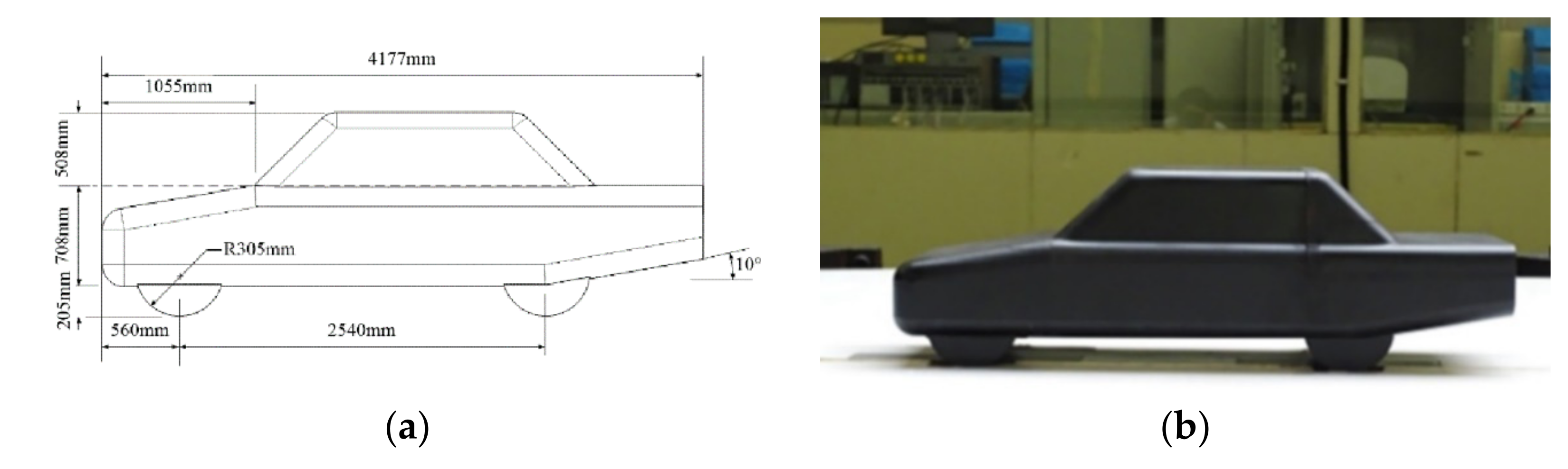
2.1. Wind Tunnel and Vehicle Model

Experiments were conducted in an open circuit wind tunnel with an 8 m-long × 4 m-wide × 2.2 m-high test section of Jilin University. The maximum speed of the tunnel is approximately 60 m/s and the nozzle area is 8.4 m². The appearance and size of an original MRIA notchback are given in Figure 1, which is 0.521 m in length (L), 0.203 m in width (B), and 0.178 m in height (H). As the experiment model size, the boundary layer of the ground may have an impact on the flow structure. Therefore, the test bench was specially made for the notchback model to avoid the above issue, with a 2.4-m-long × 1.2-m-wide × 1.0-m-high thin flat plate located in the middle of wind tunnel (Figure 2). Additionally, the notchback model was placed on the longitudinal center of symmetry with a 350 mm distance from the front edge of the flat plate. Measurements were conducted at the free stream velocity which is 27.78 m/s, whose Reynolds number Re_L is 9.16 × 10⁵, where superscript ‘L’ denotes that this value is based on vehicle length L. The effect of Reynolds number on the flow will not be researched in this paper, but some experimental work has been completed regarding the drag coefficient of the 1/8 MIRA notch at different velocities included U∞ = 16.67 m/s, 22.22 m/s, 27.78 m/s, 33.33 m/s, and 38.89 m/s. Additionally, limited drag coefficient shows a variation, albeit slightly, with increasing Re. The work suggests that the overall flow structure does not change significantly with the flow velocity, but it is uncertain that small changes in flow characteristics as a function of Reynolds number may exhibit [16]. This study will be continued in the future. The blockage ratio of the frontal surface of the model to the cross-sectional area of the wind tunnel above the flat plate was less than 1%, not exceeding 5%.

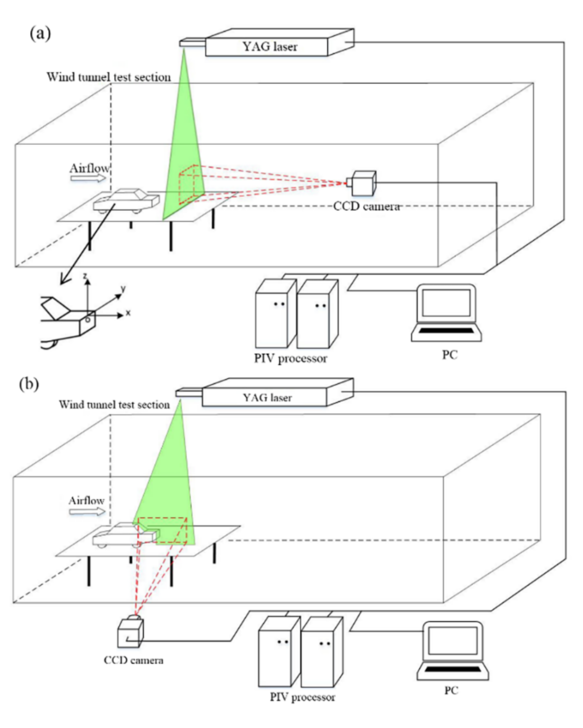
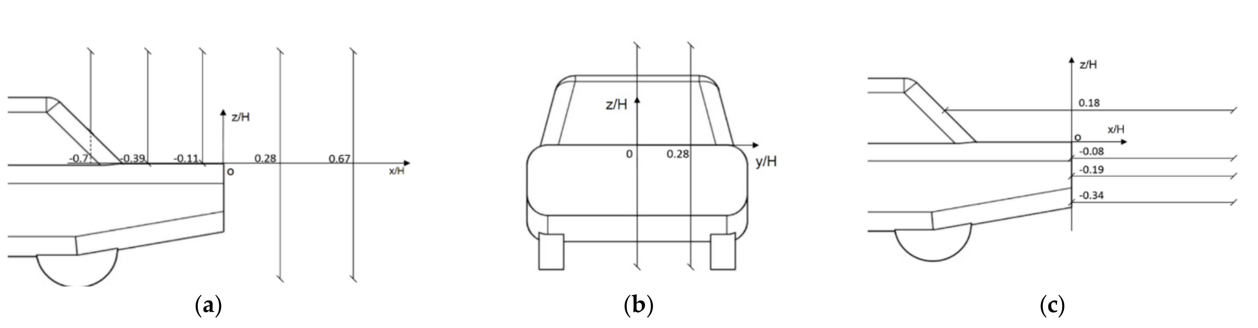
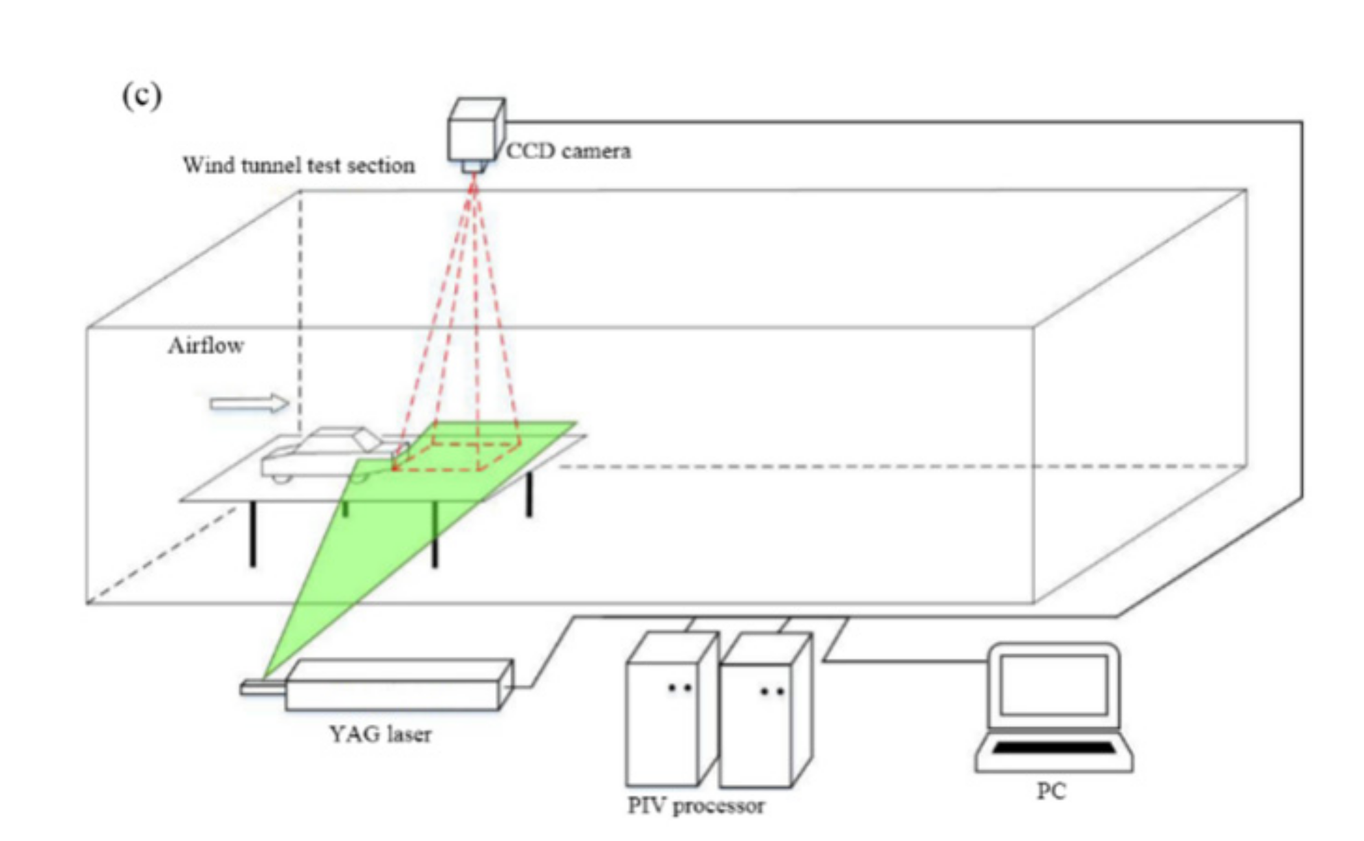
2.2. PIV Measurements

Tracing particles are seeded in the flow field equably in order to illustrate flow information. At some point, laser generator emits two pulses in a short time interval dT to illuminate the same plane which is selected to be measured, so that tracing particles can be captured by camera at the same time. With two pictures, displacement of each particle inside the plane in two orthogonality directions, Δx and Δy, can be obtained. Then, if dT can be small enough, instantaneous velocity component in x and y direction, uins and vins, would be approximate by average velocity component uave and vave, respectively, which can be calculated by the following equation:

$$\begin{array}{l}{u}_{ins}\approx u_{ave}=\frac{\Delta x}{dT}\\ v_{ins}\approx v_{ave}=\frac{\Delta y}{dT}\end{array}$$

(1)

With the velocity components calculated, vorticity is quite easy to be obtained. As we all know, vorticity is one of the most important methods to describe the swirl flows; it is rational and efficient to use vorticity as a measure of vortex identification. However, as vorticity fails to recognize the shear flow in the average processing, time-averaged velocity streamline and iso-contours of time-averaged streamwise velocity were calculated in this paper.

TSI PIV system was used to measure the flow around the notchback model. The schematic diagram of experimental setup is shown in Figure 2. The flow was illuminated using two Nd-YAG lasers, each with a maximum energy output of 200 mJ/pulse. The output beams were shaped into a 2 mm thick laser sheet normal to the free stream by a cylindrical lens. The lasers were synchronized to illuminate the flow twice, with a short time delay between the two exposures. Pulse interval value (dT) in these experiments were set to 15 µs and the time resolution of the PIV system was 3.75 Hz. The paraffin oil particles with an average diameter of 2–5 μm were released into the flow field by a smoke generator. The light scattered by the seeding particles was photographed with a CCD camera (TSI PIVCAM13-8, 1280 × 1024 pixels). The field of view of PIV images was about 350 × 300 mm. The number of images must be large enough to resolve the time-averaged and instantaneous flow fields [17]. Therefore, in total, 1200 PIV images were photographed at each plane.

Before taking these images, the length of images was marked by ruler. With images captured, cross-correlation algorithm was processed with 32 × 32 pixels in interrogation windows. Additionally, Fast Fourier Transformation was adopted with 50% overlap. In post processing, the vectors are compared against the neighboring vectors. Vectors that vary by more than the validation tolerance (default in Insight Software) from the neighborhood average, are removed. This neighborhood check enforces continuity on the flow. Places that are left empty can be filled in by interpolating the neighboring vectors to achieve the best estimate of the velocity at that point.

Figure 2 shows the definition of the right-handed Cartesian system (x, y, z), with the origin O at the midpoint of the upper edge of the model vertical base [18]. It is defined such that x, y, and z which are set up along the longitudinal, spanwise, and vertical directions, respectively. In order to capture the highly 3D flow structure accurately, PIV measurements were executed in a number of planes, including the x–z plane at y/H = 0(symmetry plane) and y/H = 0.28; the x–y plane at z/H = −0.34, z/H = −0.19, z/H = −0.08, and z/H = 0.18; and the y–z plane at x/H = −0.7, x/H = −0.39, x/H = −0.11, x/H = 0.28, and x/H = 0.67, respectively. Different measurement planes are shown in Figure 3. For the measurements in the y–z plane, a camera was vertically placed at around x = 2000 mm behind the laser sheet, and it was equivalent to 4 times of vehicle lengths. When performing longitudinal measurements, the camera effect on the flow field should be small enough.

The PIV data were processed by Insight software from TSI. Additionally, the 1200 PIV images of each plane were averaged to one time-average image.

3. Analysis of Longitudinal Structures (y–z Planes)

In the wake of MIRA notchback model, the longitudinal flow field can be discussed by observing the cross-section flow field parallel to the air flow direction, which is the most able to reflect the structure and the formation process of the flow field behind the vehicle. Additionally, a series of instantaneous flow field shows a very complex, random variation of the vortex structure and vortex formation, shedding process, which cannot be seen from time-averaged flow field, while the time-averaged flow field shows a stable and complete vortex structure that is also useful for the analysis of instantaneous flow. Therefore, the instantaneous flow information of five different cross-sections was also collected at the longitudinal direction.

3.1. Time-Averaged Flow

Time-averaged flow were obtained by averaging the 1200 images captured. Figure 4 shows the iso-contours of time-averaged streamwise vorticity ω in the y–z plane at x/H = −0.7. A solid line means positive vorticity rotating counter-clockwise. A dashed line means negative vorticity rotating clockwise. We can attribute the half-baked line to the intersecting of the cross-section and the model body. There is a pair of small counter-rotating vortices marked with C appearing on both upper sides of the C-pillar of the vehicle. As the airflow flows through the C-pillar, the airflow from the body side forms a separated shear layer over the C-pillar and rolls up into cone-shaped, streamwise vortices which can also be seen in Figure 5. This is the beginning of the formation of the well-known C-pillar vortices.

As shown in Figure 5, Figure 6 and Figure 7, the size of the C-pillar vortex further enlarges while moving backward from x/H = −0.7 to x/H = −0.11, and the vorticity increases by more than 200 %. At the same time, the locations of vortex cores are downward tilted from z/H = 0.23 to z/H = 0 with increasing x due to the flow separation and the effect of downwash flow. Moreover, in the next Figure 7 and Figure 8, these vortices grow in both vorticity strength and size while running downstream, and then form a pair of long drag vortices. Eventually, the pair of counter-rotating vortices decays in the far wake.

Besides the C-pillar vortex, another pair of interesting vortices appears below the upper edge of the back window and above the C-pillar vortex, shown in Figure 5 and marked by A. As the flow from the front of the wind shield separates from the A-pillar, it forms the A-pillar trailing vortices. These vortices trail along the side glass and move over the roof, then appear in the wake above and inside the C-pillar vortices (Figure 6 and Figure 7). The shape of the autobody can make a great influence on the development and movement of A-pillar vortices [15,19].

As a result of the interference of both the airflow from body sides and the wash airflow from body bottom occurs at the rear wheels at x/H = 0.28 (Figure 7), it causes airflow separation and merging, resulting in a very complex vortex structure behind. Firstly, a pair of vortex structures marked by E are captured in the middle of the vehicle tail. Ahmed researched that a separation occurring at the blunt edges of the body forms a recirculation region characterized by two small inner vortices, a so-called recirculation bubble A and B (not shown), which is formed by the inner part of shear layers rolling up from the upper and lower edges of the vehicle base [20]. As shown in Figure 7, the mechanism of vortex E is same as the recirculation bubble A, which is formed by the downwash shear layer rolled up from the trunk deck, and the downward trend of the C-pillar vortex forces vortex E to the middle location of the tail. Combining with the vertical section in Figures 16 and 17, and the vertical section vortex structure in Figure 27, we can see that the shape of vortex E shows a pair of L type, and the size of vortex, from the vertical tail center to the side of the body, becomes gradually smaller, as shown in Figure 9. The C-pillar downwash vortex squeezes both the side vortex and vortex D, mentioned later.

However, in Figure 7, there is not a complete vortex similar to vortex B of Ahmed model [19]. On the contrary, there are many vortices (marked with F) around the lower edge of the tail, which tend to occur alternately and be aligned in a row.

Likewise, as a result of the tail upturn angle, a new pair of highly concentrated, counter-rotating, large-scale vorticity appear, marked by D in Figure 8, which are similar to the C-pillar vortex and have not been researched in detail to date. They come from the merger of shear layers from tail upturn angle and body side, then extend and develop into a pair of longitudinal trail vortex. The vortices D are located at the lower end of the C-pillars vortex, which is weaker in vorticity strength and smaller in size than C-pillar vortex. Moreover, the rotation direction of vortex D and the C-pillar vortex are contrary. Nevertheless, the C-pillar vortex and vortex D also have interaction and influence in the process of their formation and development, which will be described later. In addition, one vorticity concentration, marked by I, appears around vortex D, along each side surface of the model, which probably results from the shear layer developed over the side surface of the model and merges with vortex D and vortex I gradually.

Finally, there are also some interesting vortex structures developed at the vehicle underside clearance and the rear wheels. In Figure 7 and Figure 8, we can see there is a pair of vortices G between the ground and the model underside, which is related to the shear layer flow, apparently slowed down in the gap, leading to the pressure difference inside and outside of the gap. In the end, the shear layer rolls up to a pair of longitudinal vortices G. The maximum vorticity concentration of vortices G is about 25% of the C-pillars’ and it gradually merges with vortex D.

3.2. Instantaneous Flow

From Figure 10, one row of small, alternately signed vortices occurs at the upper edge of the back window, and develops downstream gradually in Figure 11, which does not appear in the time-averaged flow field shown in Figure 4 or Figure 5 due to the fact they tend to offset one another in the averaging process. As shown in Figure 12a, its characteristics are similar with a spanwise roll vortex wrapped with the rib structure on the upper edge of Ahmed model, with the slant of α = 35° [17]. It occurs due to the flow separation from the upper edge of the back window and is absorbed by the A-pillar vortex gradually, in the process of extending downward, as seen in in Figure 13.

The C-pillar and A-pillar vortices are identified easily with a pair of the most highly concentrated, counter-rotating, large-scale vortices in Figure 13. These results indicate that the longitudinal structures are very stable in space. Additionally, we can also find that the maximum instantaneous vorticity concentration of the C-pillar and the A-pillar is greater than the time-averaged one. The instantaneous flow is characterized by chaotic variation in order, and it represents just a certain moment of vorticity rather than the average vorticity of a period of time.

Typical instantaneous vorticity at x/H = 0.28 is exhibited in Figure 14. The main features are consistent with the time-averaged flow shown in Figure 9. Firstly, the shape and location of the C-pillar and E vortices are similar. The maximum vorticity concentration of the C-pillar vortex is quite high, but the size is not large and resembles a strip. This due to the separation of A-pillar after leaving the model, resulting in the vorticity of fluctuation being counteracted while averaging. Secondly, there is a row of small, dispersed vorticity concentrations occurring on the lower edge of the model, which is consistent with its counterpart in Figure 7, implying that the vortices F structure is closely affected by vortex E, and its feature is a wavy, spanwise roll with the rib structure in Figure 12b. The influence from vortex D also cannot be ignored. However, the tail upturn angle may be the most important factor leading to the F vortex structure. Although the vortices under the model are very messy, the structure of vortex D is visible.

As shown in Figure 14, the instantaneous flow seems to be random, but reveals the leaves out of the back window interaction relationship between the C-pillar vortex and vortex D. We can see that the vortex core of the C-pillar is surrounded by many small positive and negative vortex structures, and vortex D is scattered. To take the right part vortices of Figure 15 as an example, the C-pillar vortex and vortex D are counter-rotating. At the junction of the two vortices occurs a strong interlacing, leading to many respective sub-vortices. Moreover, as the size and vorticity of the C-pillar vortices are much larger than vortex D, it plays a dominant role relative to vortex D, and the C-pillar vortex cores are rounded by most of the sub-vortices. Additionally, the two C-pillar vortices may also separate and generate sub-vortices. Therefore, it can be seen that the C-pillar vortex and the D vortex extend in opposite directions in the longitudinal direction, accompanied by mutual shearing action. The analysis of the instantaneous flow unveils the formation and detachment of the vortex, which makes us understand the formation mechanism of the vortex more clearly.

4. Analysis of Spanwise Structures (x–z Planes)

4.1. Time-Averaged Flow

As shown in Figure 16 and Figure 17, we can clearly see the flow characteristics of spanwise structurers near wake. The airflow over the roof of the model separates at the upper edge of back window. Then, the airflow leaves from the back window and develops into a long downwash flow. Observing the shape of this vortex in Figure 16 and Figure 17, the characteristic of middle part is thick and long, but vortices at both sides are thin and short. This phenomenon may be closely connected with the C-pillar vortex and the A-pillar vortex.

As the separated shear layer reattaches to the back window, it produces a big recirculation region (Figure 18). (It seems that the streamlines protrude into the geometry, which can be explained by the errors of PIV data acquisition. On the other hand, some extensions or deviations may be possible while drawing curves.) There are some small vortices below the recirculation zone marked by hairpin vortex R (Figure 16). These vortices are driven by the shear layer.

Additionally, in Figure 16, vortex E begins to extend down from the upper edge of trunk deck. Meanwhile, it appears to present a triangle vortex occupying 2/3 of the wake region. However, on both sides of the trunk deck (Figure 17), the shape of vortex E presents a strip structure, and the vorticity strength is also reduced. In addition, along the tail upturn angle, the airflow separating and rolling up forms a long vortex structure (Figure 16). However, it undergoes a rapid decrease in terms of the maximum vorticity and length of the concentration (Figure 17). The variation in shape and the vorticity strength of these vortices is due to the C-pillar as well as the A-pillar absorbing the part of vorticity. It is worth noting that vortex ‘E’ produces a much stronger vorticity concentration on the x–z plane than on the y–z plane (Figure 7). This indicates that its structure is mainly in the spanwise orientation.

Similar to the averaged velocity streamlining at y/H = 0 exhibited in Figure 18, two different recirculation bubbles appear behind the model tail, which separate from the upper and the lower edges and are called the vortices E and F, respectively. However, in the iso-contours of time-averaged streamwise velocity at y/H = 0 (Figure 19), there only exists one large recirculation bubble with very low velocity; the other has disappeared. Therefore, it is evident that vortex E accounts for a leading role in wake and influences the development of vortex F.

Finally, in Figure 16, there is a very long vortex structure behind the wheel, which is vortex G. It has a great impact on the development of the C-pillar vortex, and even the entire wake flow field.

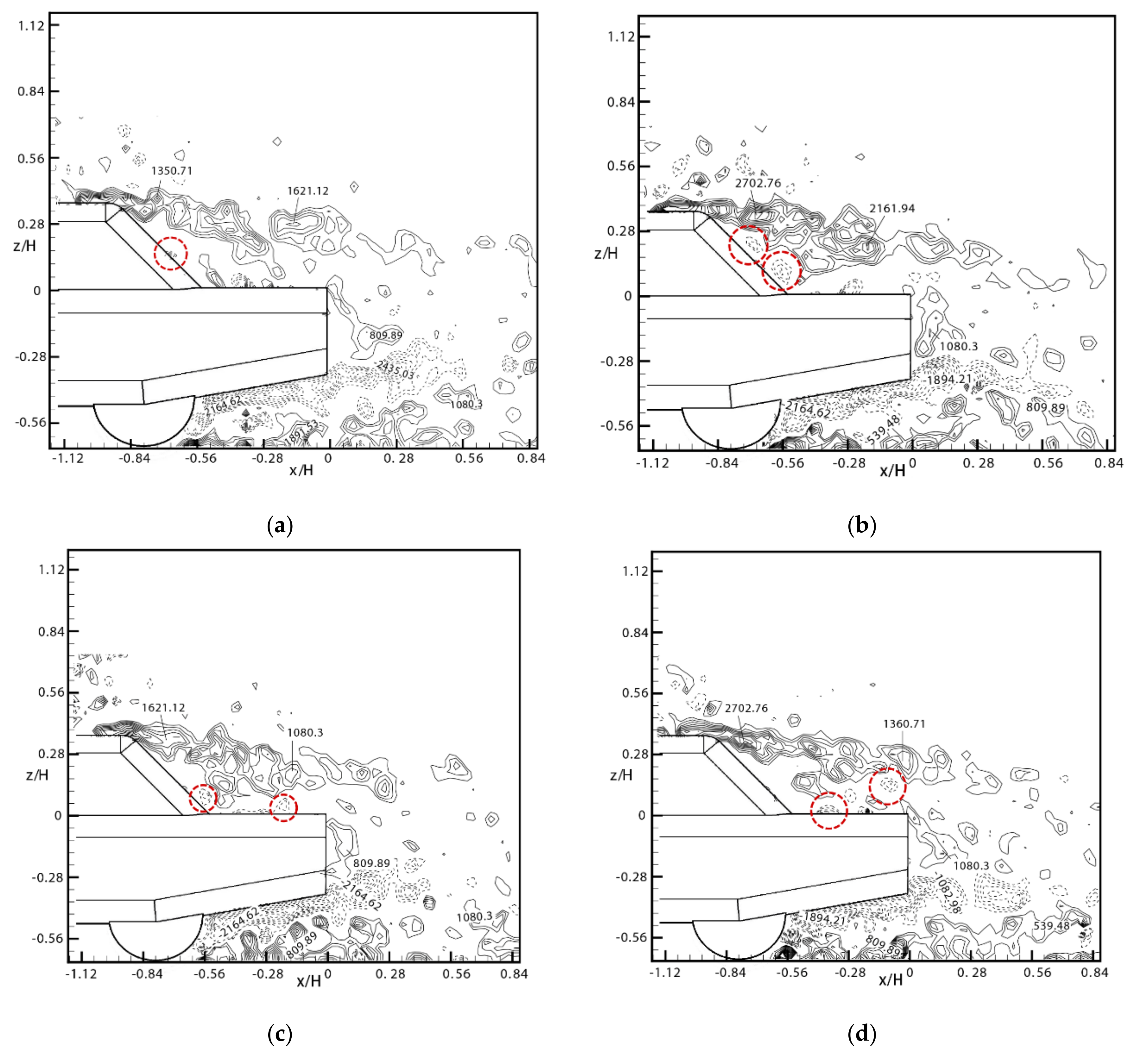
4.2. Instantaneous Flow

The hairpin vortex on the back window seems to be very stable circulation vortex. In fact, it has a certain formation and shedding cycle, which is presented in instantaneous flow field. Figure 20 (not consecutive in time) illustrated a certain time of continuous instantaneous vorticity. In picture (a), a small vortex highlighted by a red-colored broken forms in the early period. With the shear layer rolling up from the back windows, two circulation vortices grow up and appear on the back window shown in picture (b), then they reattach to the deck lid and move backward gradually in picture (c). Next, the vortices leave out the deck lid and, one by one, disappear in the wake, shown in pictures (d) and (e). Finally, another new vortex appears in the picture (f) as the previous separation. It is deduced that a new vortex reforms on the back window only after a vortex shedding from the deck lid.

As shown in Figure 21, in the continuous variation of the instantaneous flow, some typical characteristics of vortex structures are similar with the time-averaged feature, such as vortex E but, in fact, they are in a cycle of forming, shedding, and disappearing.

Figure 21 shows representative instantaneous vorticity in the near wake of the x–z plane at y/H = 0.28, which is similar to the x–z plane at y/H = 0 and unveils some interesting phenomenon. The downwash airflow over the roof reattaches to the deck lid and absorbs vortex E, so that there is no obvious vortex structure behind the tail. Meanwhile, the upwash airflow under the model crashes the downwash flow at x/H = 0.28 acutely, generating some separation vortices. According to the above analyses, the formation and development of vortex E mainly occurs at y/H = 0. Both the downwash flow and the C-pillar vortex have strong impacts on vortex E.

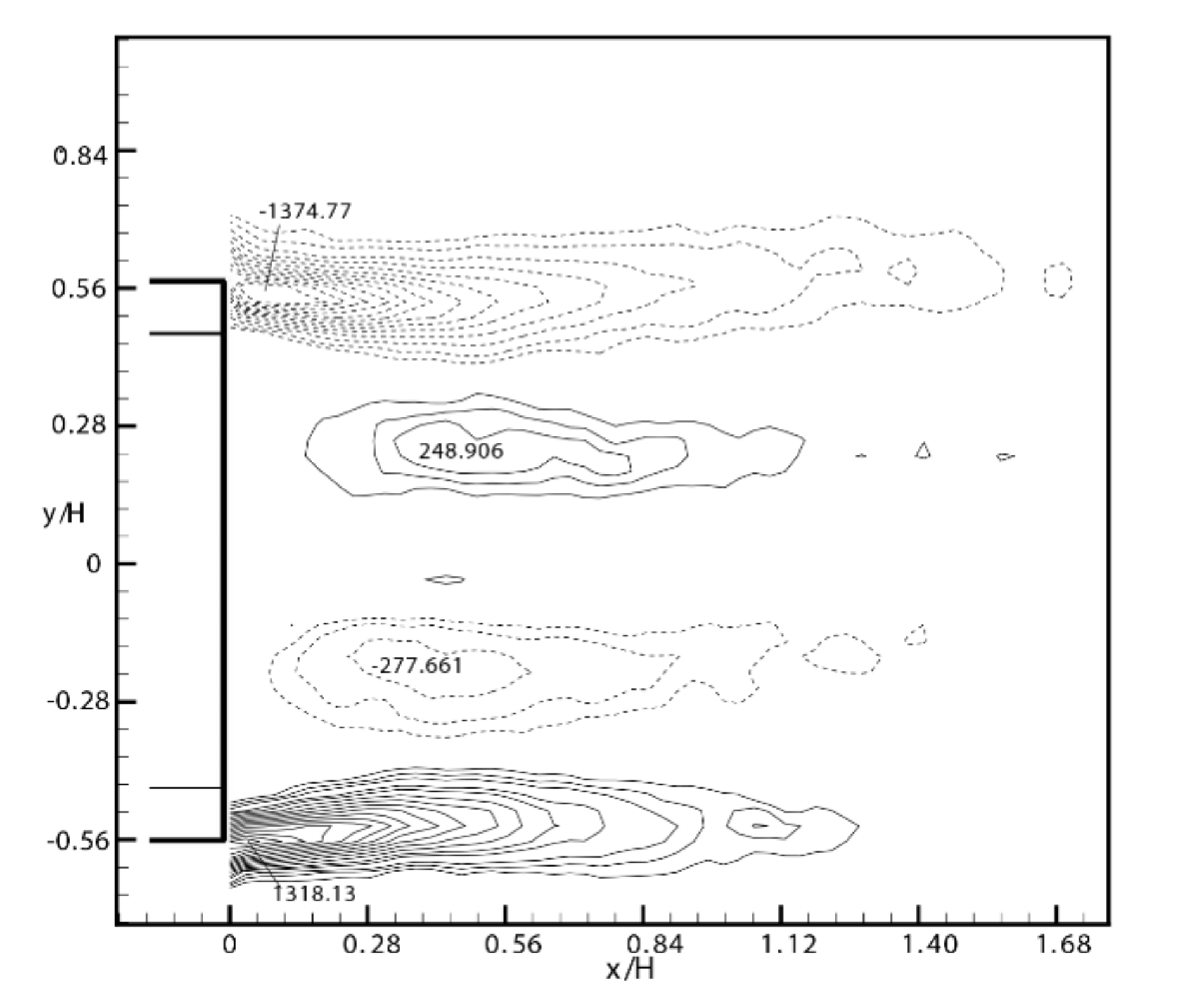
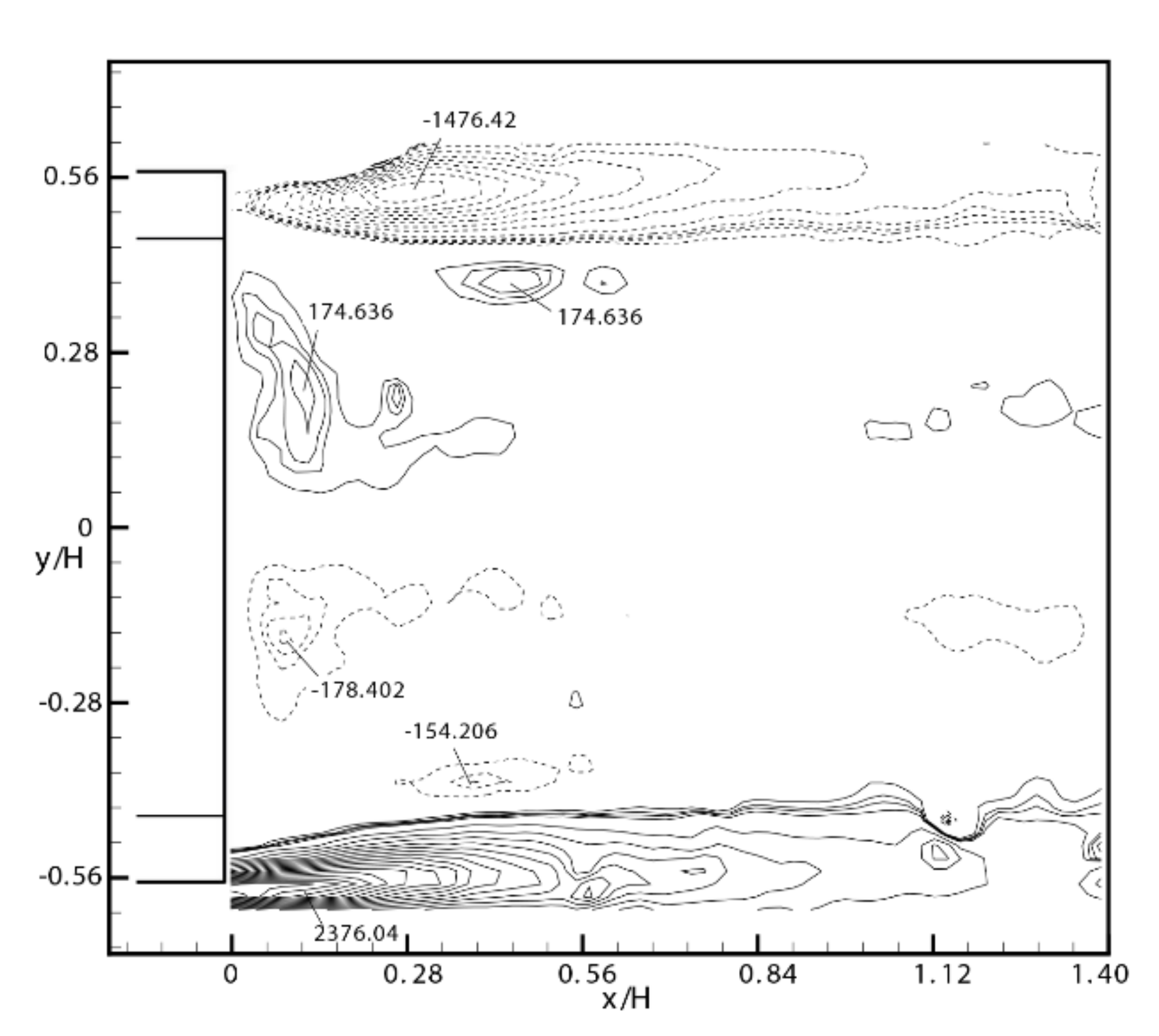
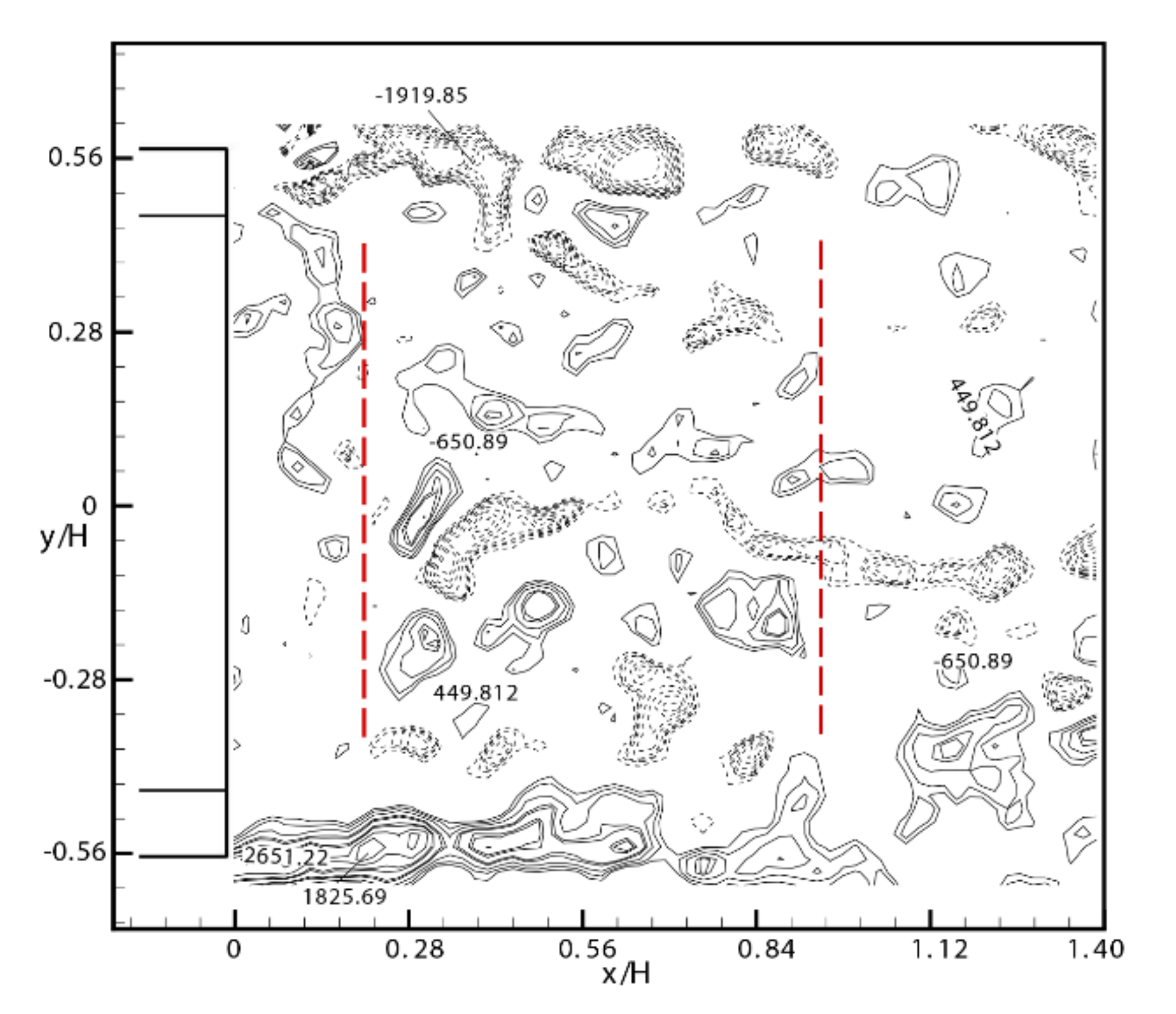
5. Analysis of Vertical Structures (x–y Planes)

5.1. Instantaneous Flow

The iso-contours of instantaneous vertical vorticity ωz in the x–y plane at z/H = 0.18 (Figure 22) shows that the shear layer from both sides of the cabin makes a separation, and some part of the shear layer is involved in the formation of C-pillar vortex. Some part of the shear layer merges with the separation flow coming from the roof, which generates a big recirculation region behind the back window, as shown in Figure 16. The last part of the shear layer connects with the A-pillar vortex. From Figure 22, we can find the airflow on both sides moved gradually to the middle by the pushing from the development of the C-pillar vortex which is similar with the flow path of the A-pillar. Therefore, it is inferred that the airflow merges together with the A-pillar vortex making the size and vorticity strength of the A-pillar vortex larger and stronger (Figure 6). Subsequently, the A-pillar vortex becomes a pair of small vortices in Figure 7. At last, the A-pillar vortex goes down and disappears in the C-pillar vortex resulting from the pushing of downwash flow. In addition, in Figure 8, we can still find the weak A-pillar vortex appears at x/H = 0.67, which indicates that the A-pillar vortex may also has a long tail.

Observing Figure 22 again, the right side shows four alternately signed vertical vortices behind the tail, which corresponds well to Figure 14. That is the instantaneous feature of the A-pillar vortex. Additionally, a series of vortices with alternating directions of rotation appears behind the back window, which are just the vortices, highlighted by thick red broken line, which appeared in Figure 11, proving the existence of a spanwise rib structure.

As in the y–z plane at z/H = −0.08 (Figure 23), the instantaneous flow structure seems complicated. There are two vorticity strips with higher energy on the sides of the model, which are located at y/H≈−0.56 and 0.56 symmetrically, apparently corresponding to vortex I (Figure 8). The strip structures appear to break down into some patches. This is likely due to the interaction with the C-pillar vortices and vortex D. It is worth noting that those patches may be the separation vortices around the C-pillar vortex in Figure 15, and vortex I is also involved in the interlacing between the C-pillar vortex and vortex D mentioned above. A row of strip vortices marked by dotted line tends to occur alternately on the inner side of position of the A-pillar vortices due to the interactions between the C-pillar vortex and vortex E, possibly also influenced by vortices I on sides. The strip vortices not only extend streamwise, but also develop downward with the increasing x.

Compared with Figure 23, the vortices structures in Figure 24 are more complex. The same is that two highly concentrated vorticity strips appear in the same location. The difference is that the alternating band vortex on the inner side of the tail obviously increases, due to the effect of vortex D, the C-pillar vortex, and vortex E, etc.

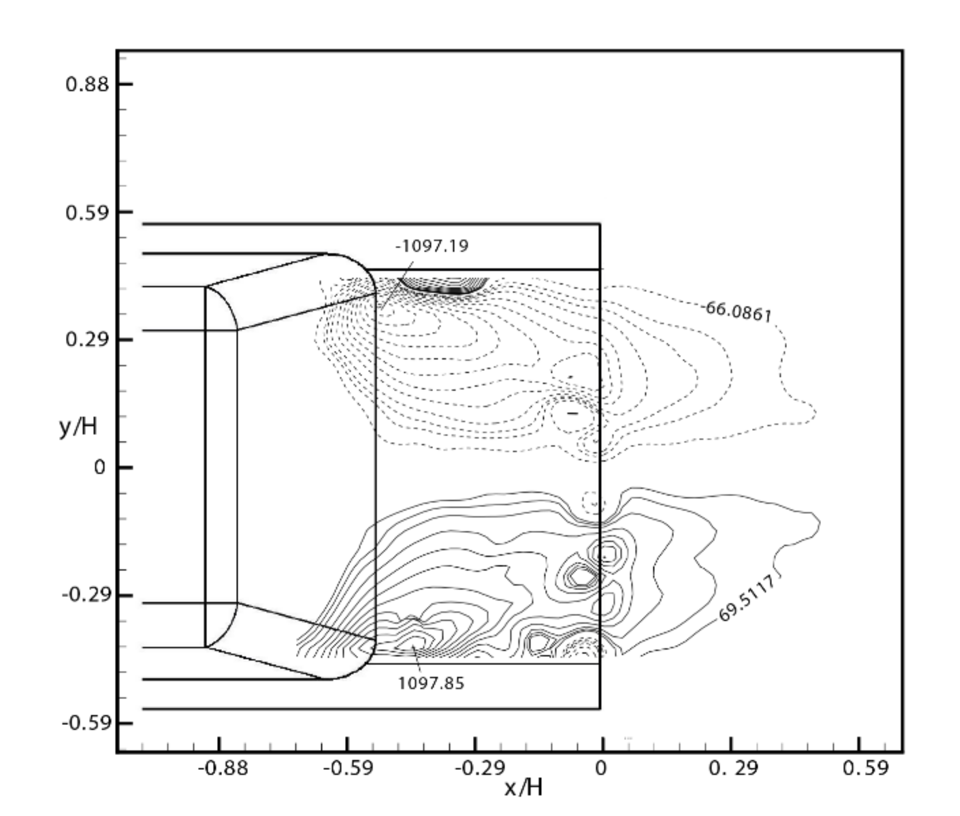
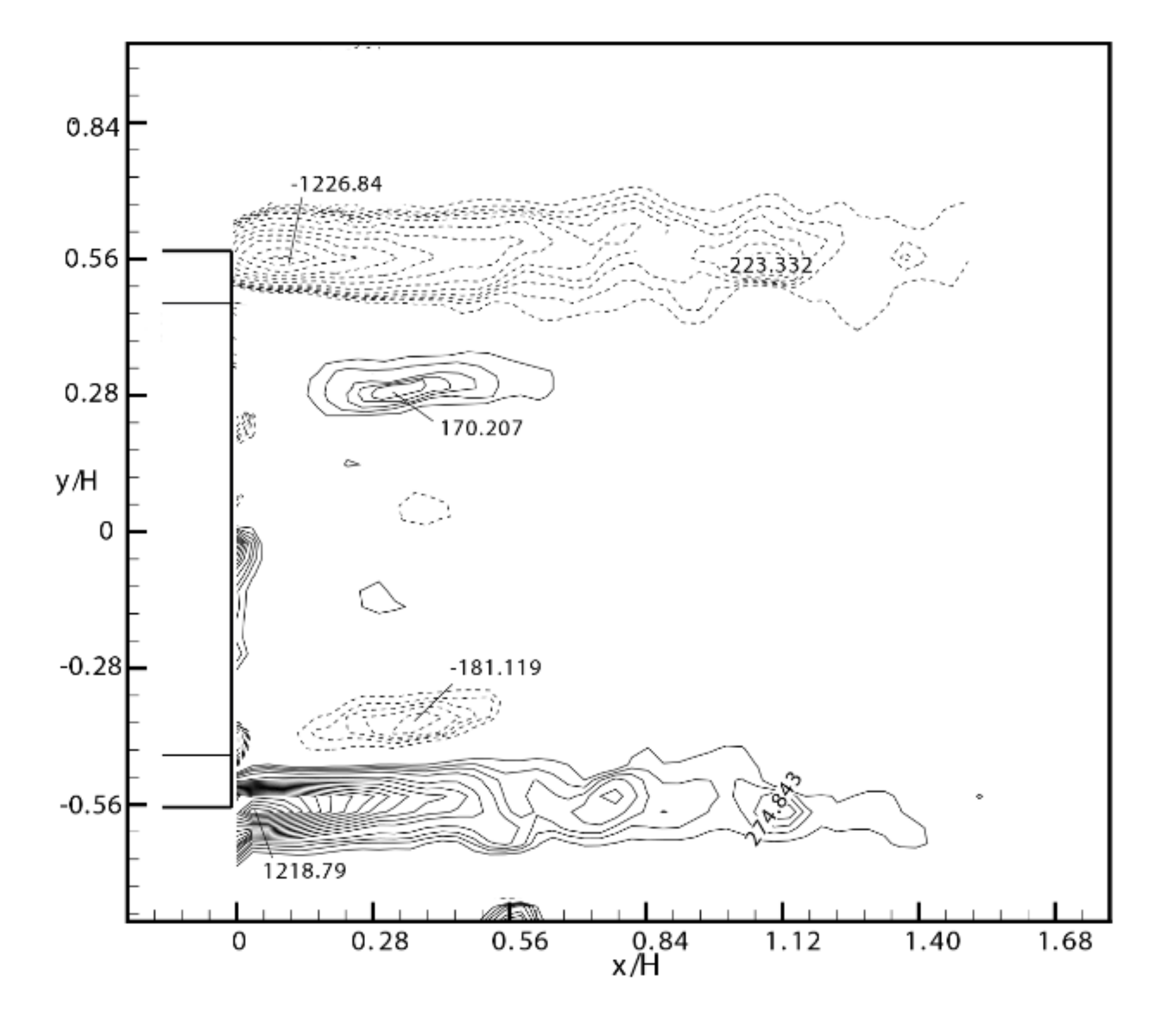
5.2. Time-Averaged Flow

The corresponding mean vorticity field can be explained in consideration of the instantaneous vertical structures. In all cases, the iso-contours of time-averaged vorticity ω in the x–y plane are approximately symmetrical about y/H= 0. In Figure 25, it can be seen in to two large vortices behind the back window, covering the whole deck lid.

In Figure 26, two strip structures are shown on each side of y/H = 0. The outer strip structures resulted from vortex I and then gradually merge with the C-pillar vortex. The inner strip structures in the opposite direction may be due to the interaction of the C-pillar vortex and vortex E, but the influence from I could not be excluded. There is a blank area between the two inner strips.

In Figure 27, the x–y plane at z/H = −0.19, the outer strip shows about 250 s⁻¹ higher in vorticity strength, and still results from vortex I. However, the end of the outer strip merges with vortex D. Near the outer strip there is a small vortex which, associated with the C-pillar vortex, may be also the inner strip in Figure 26. In addition, there are two vortices with L style in the tail of model. They clearly come from vortex E, supporting the assertion that vortex E occupies a large part of the model tail, and vortex F does not completely appear behind the model tail in Figure 28. It must be explained that, in Figure 27, as the PIV experiment has a bright spot on the model at y/H = 0.56, the data regarding vortex I at y/H = 0.56 were affected slightly. However, the wake structure is symmetrical with the flow structure at y/H = −0.56, and it does not affect the characteristics of other vortices in the graph.

In Figure 28, it is similar with the structure in Figure 26. The outer strip mainly originates from vortex I and the interaction between vortex I and vortex D. The inner strip structure is determined from vortex I and vortex D.

6. Conclusions

The wake flow of the 1/8 scale MIRA notchback model has been investigated in detail using the PIV method to obtain complete pictures of both the instantaneous and the time-averaged flows in three orthogonal planes. The investigation not only revealed the unknown instantaneous flow around the notchback, but also enriched our knowledge of the time-averaged flow, as seen in the summary and induction in the schematic of the flow structure in Figure 29. The analysis and part of the flow mechanism are summarized as follows:

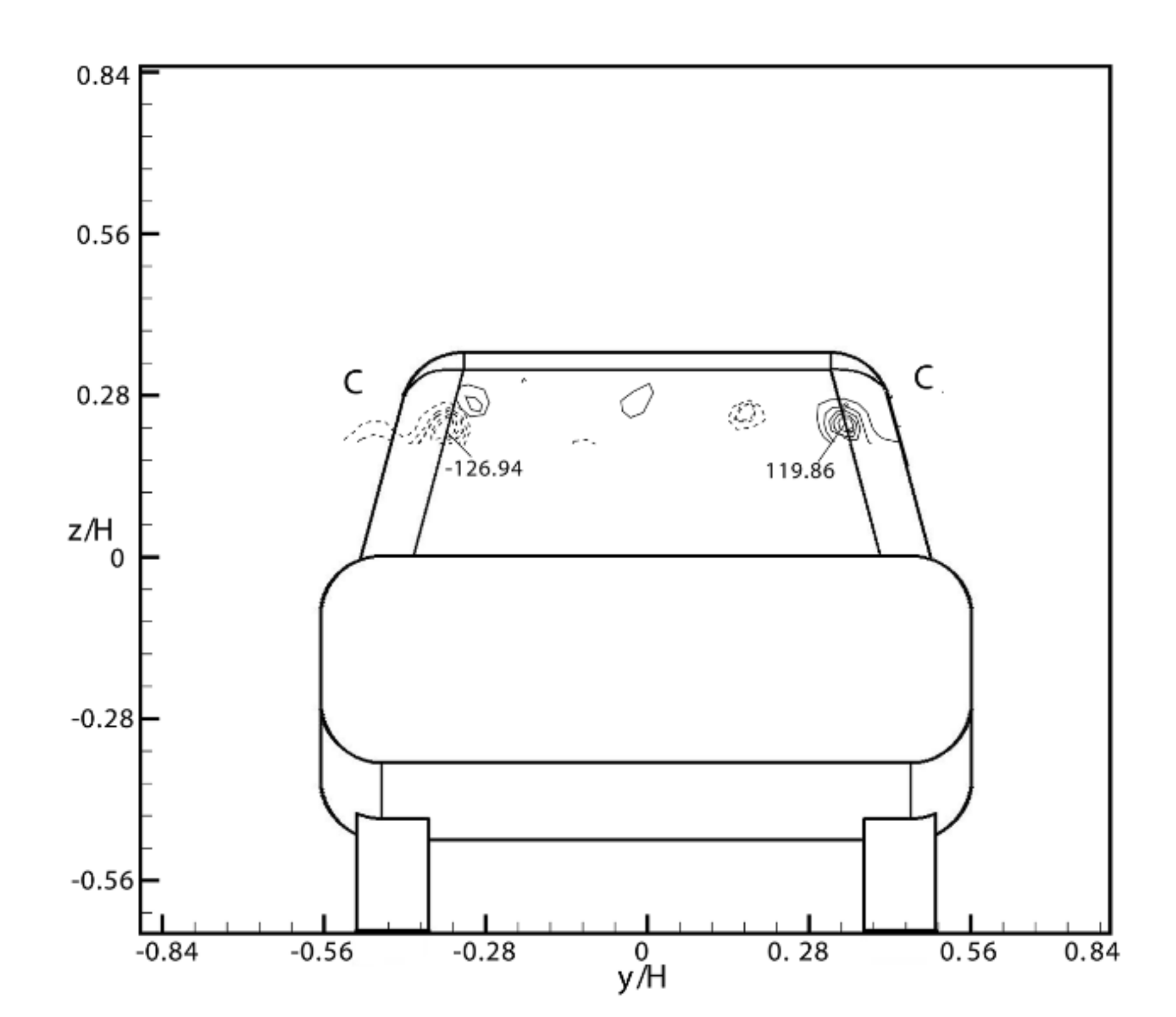
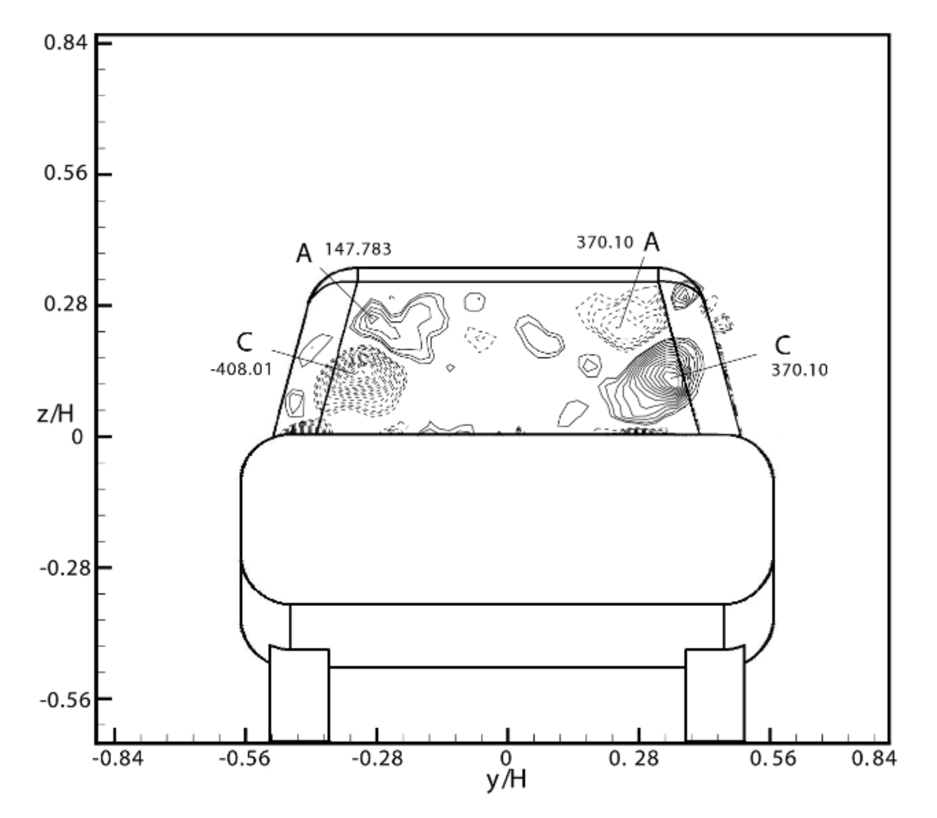
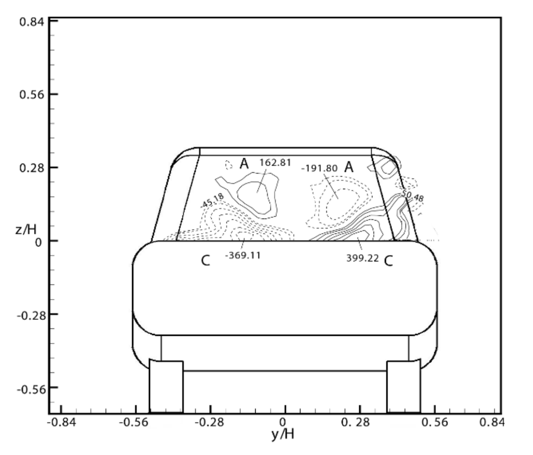
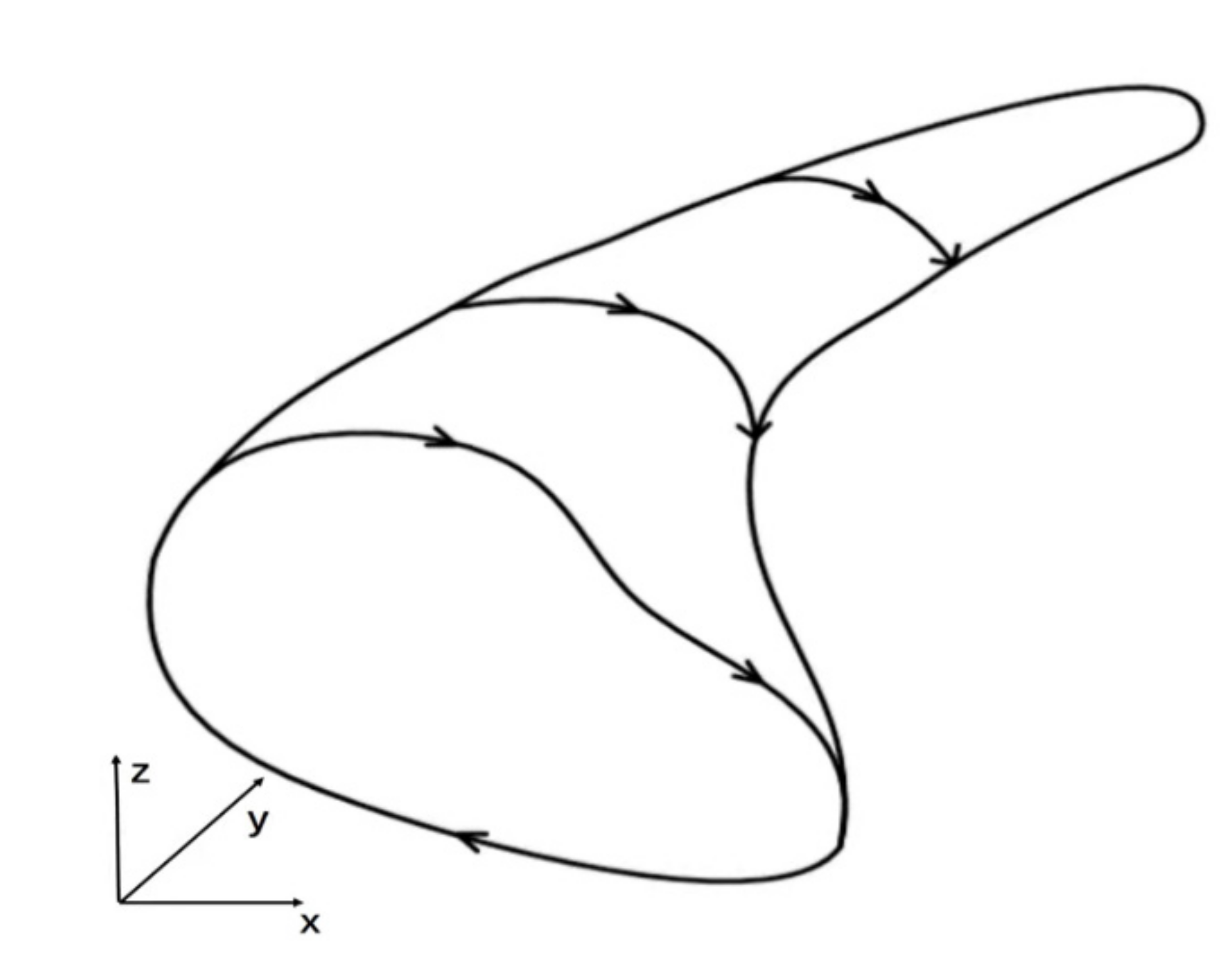
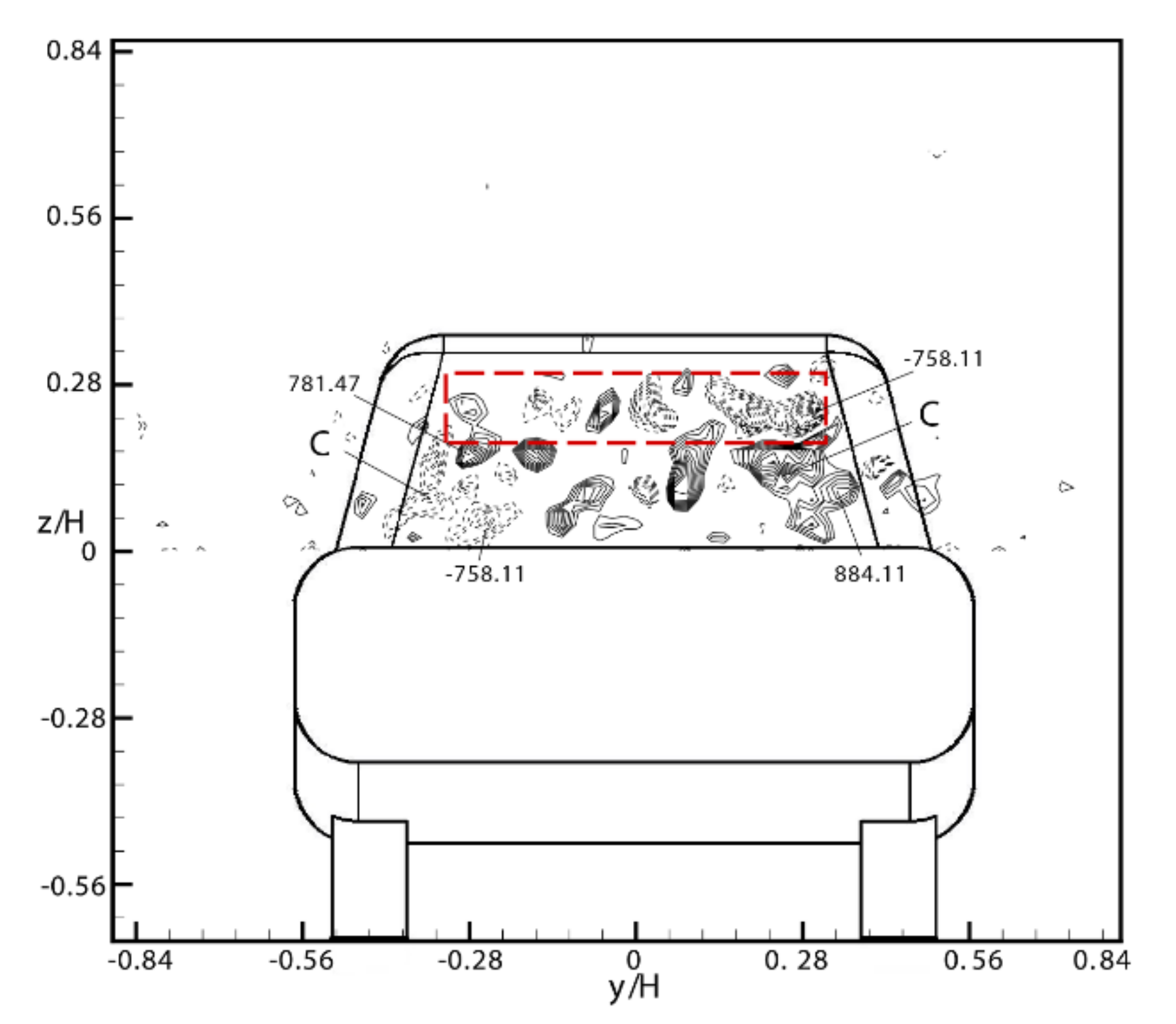
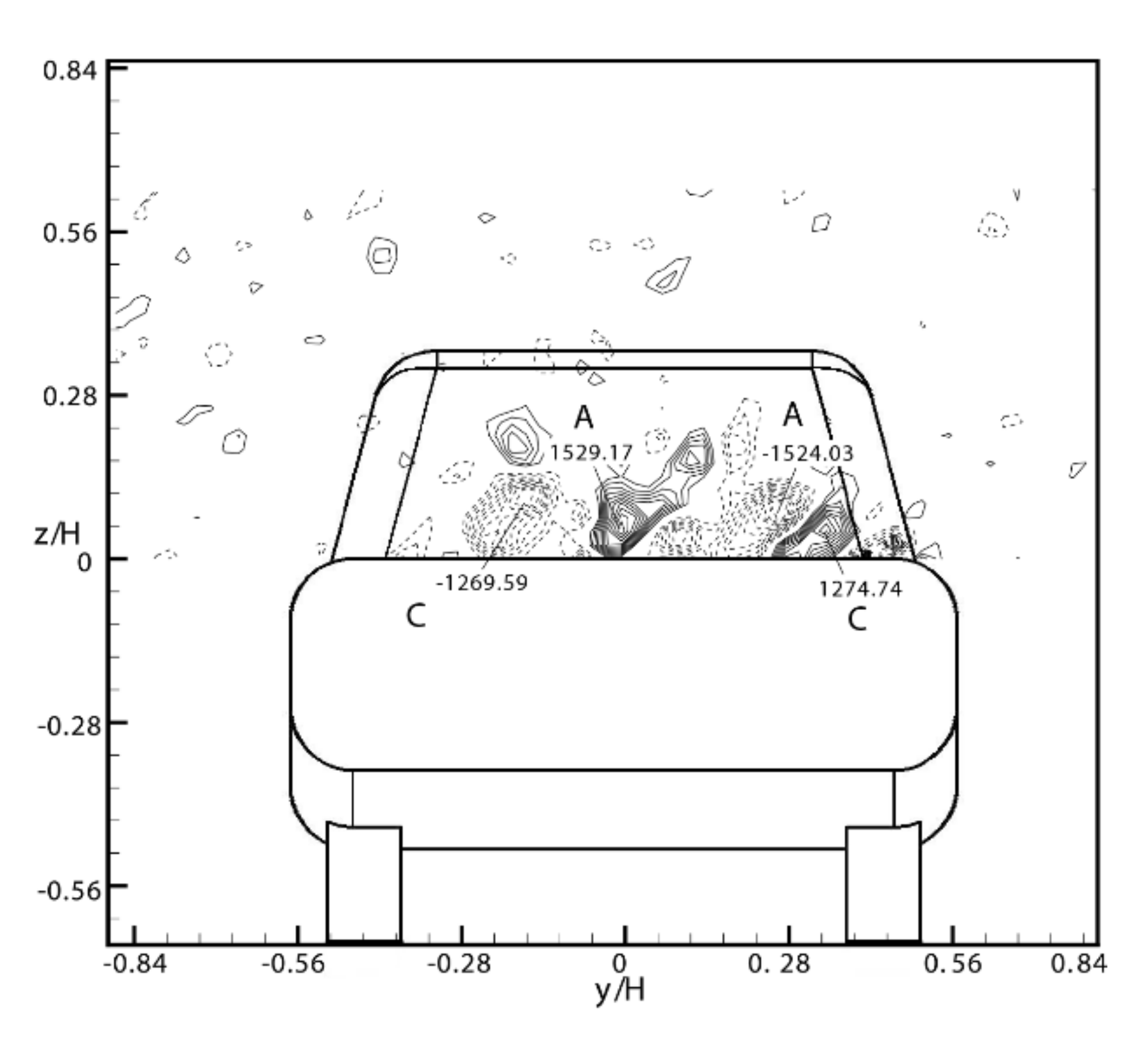
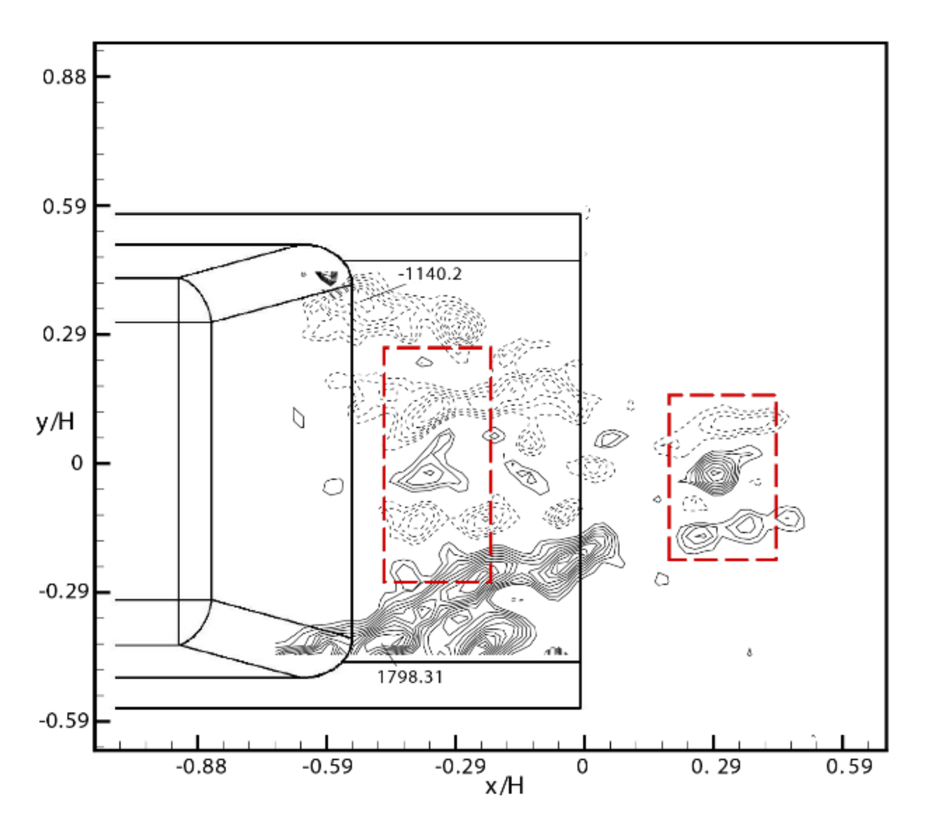
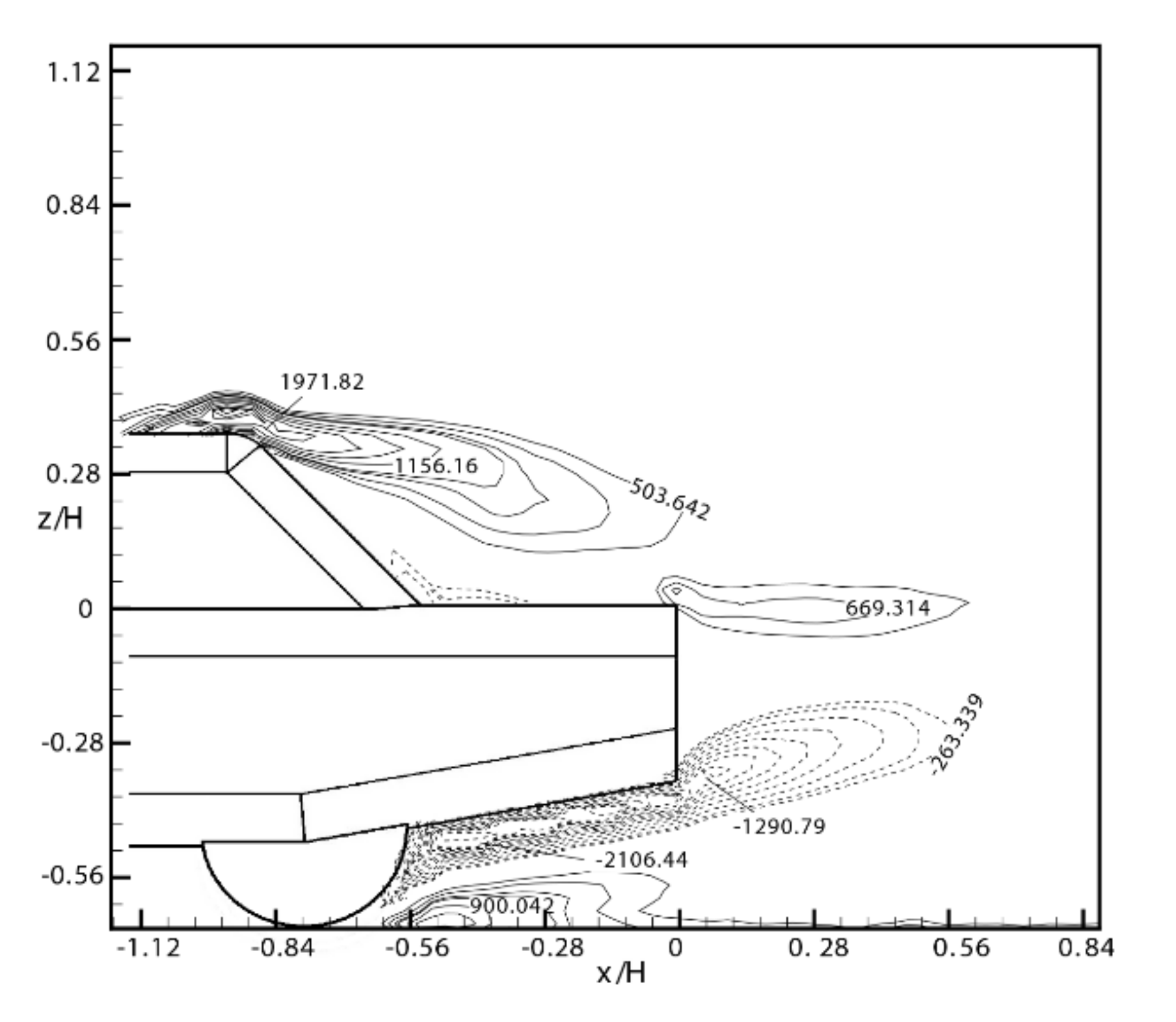
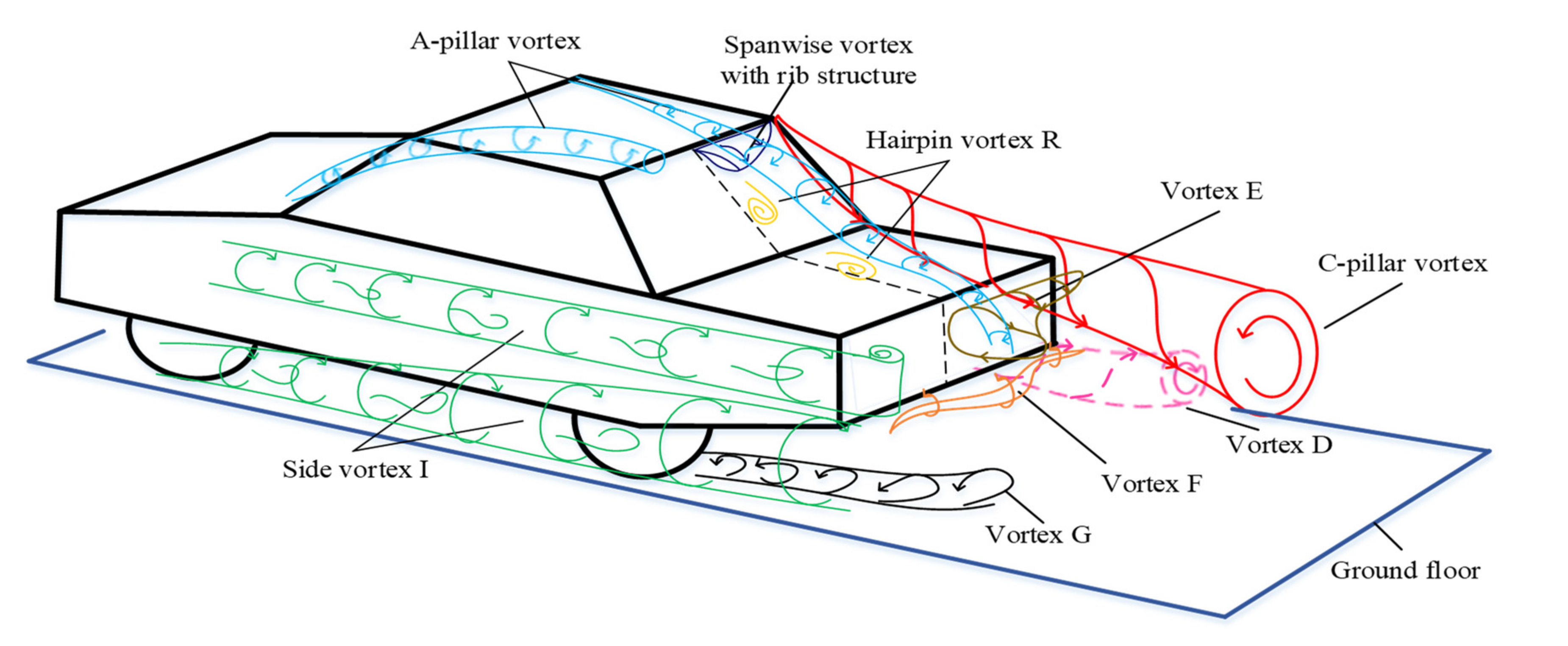
• A-pillar vortex extends backwards along both sides of the roof and meets with shear airflow on both sides of the body at the back. A pair of longitudinal vortices with small scale forms and then moves toward the middle of the tail under the compression of the C-pillar vortex. Finally, under the action of the downwash airflow, it flows into the tail flow and disappears;
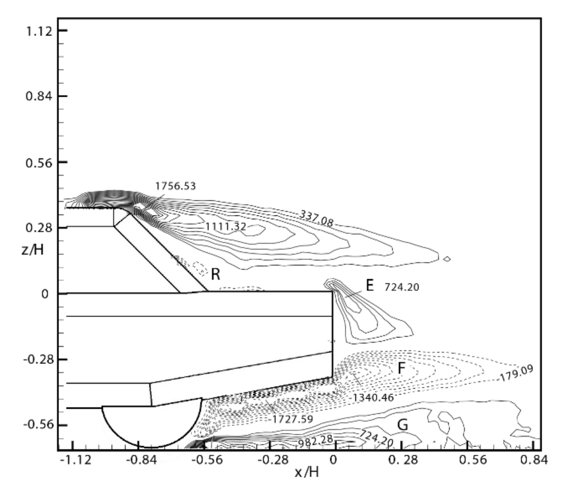
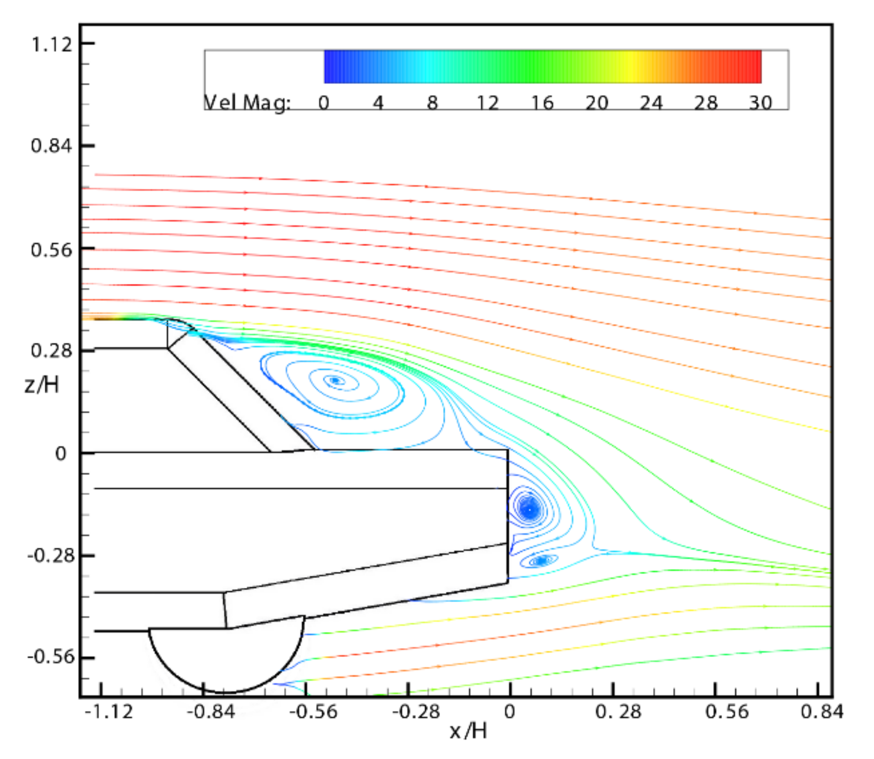
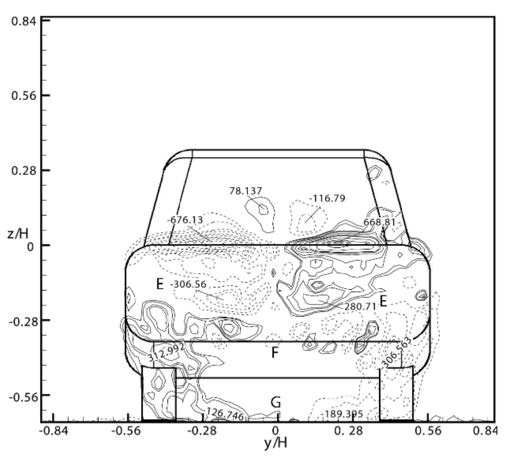
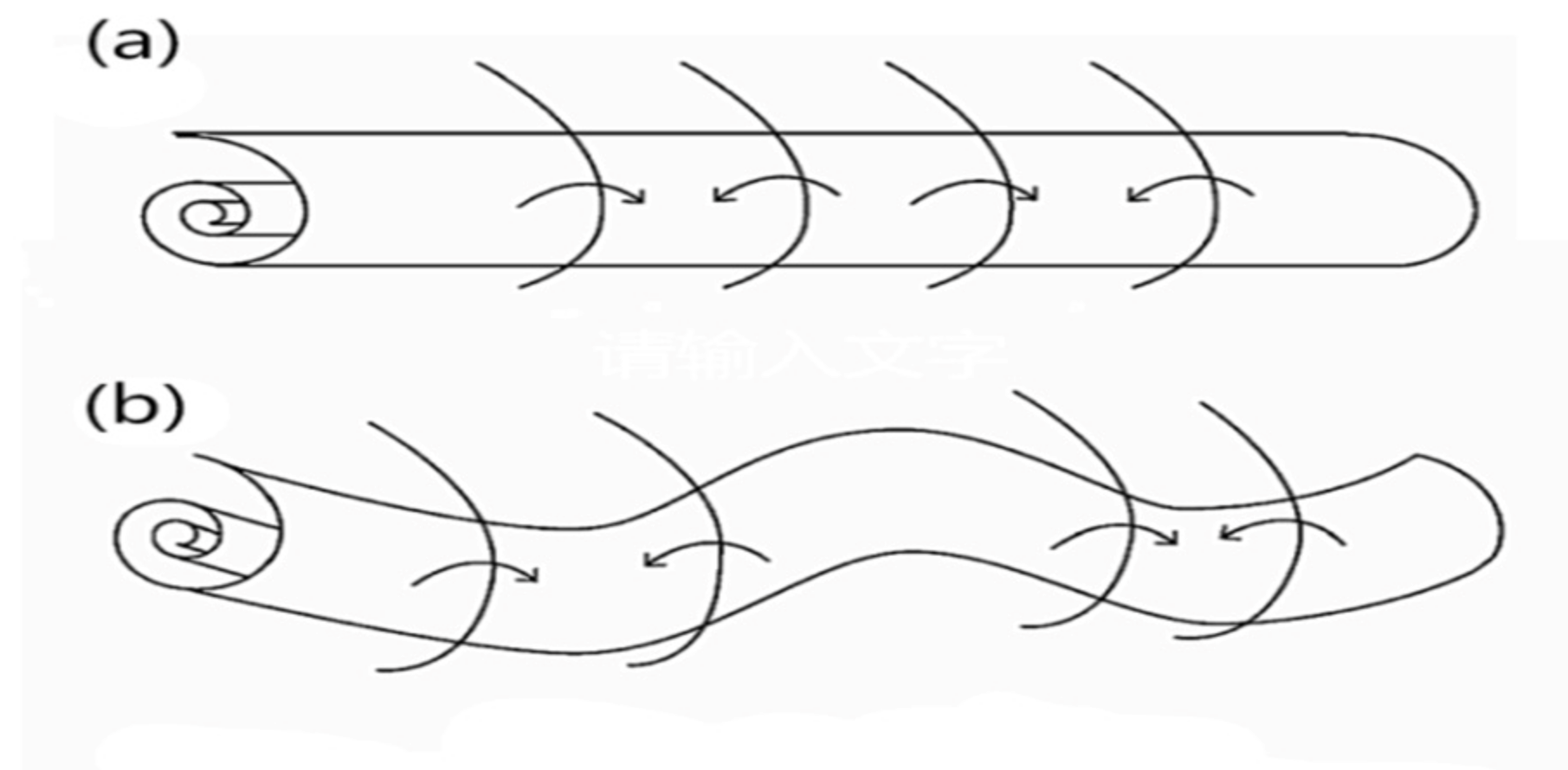
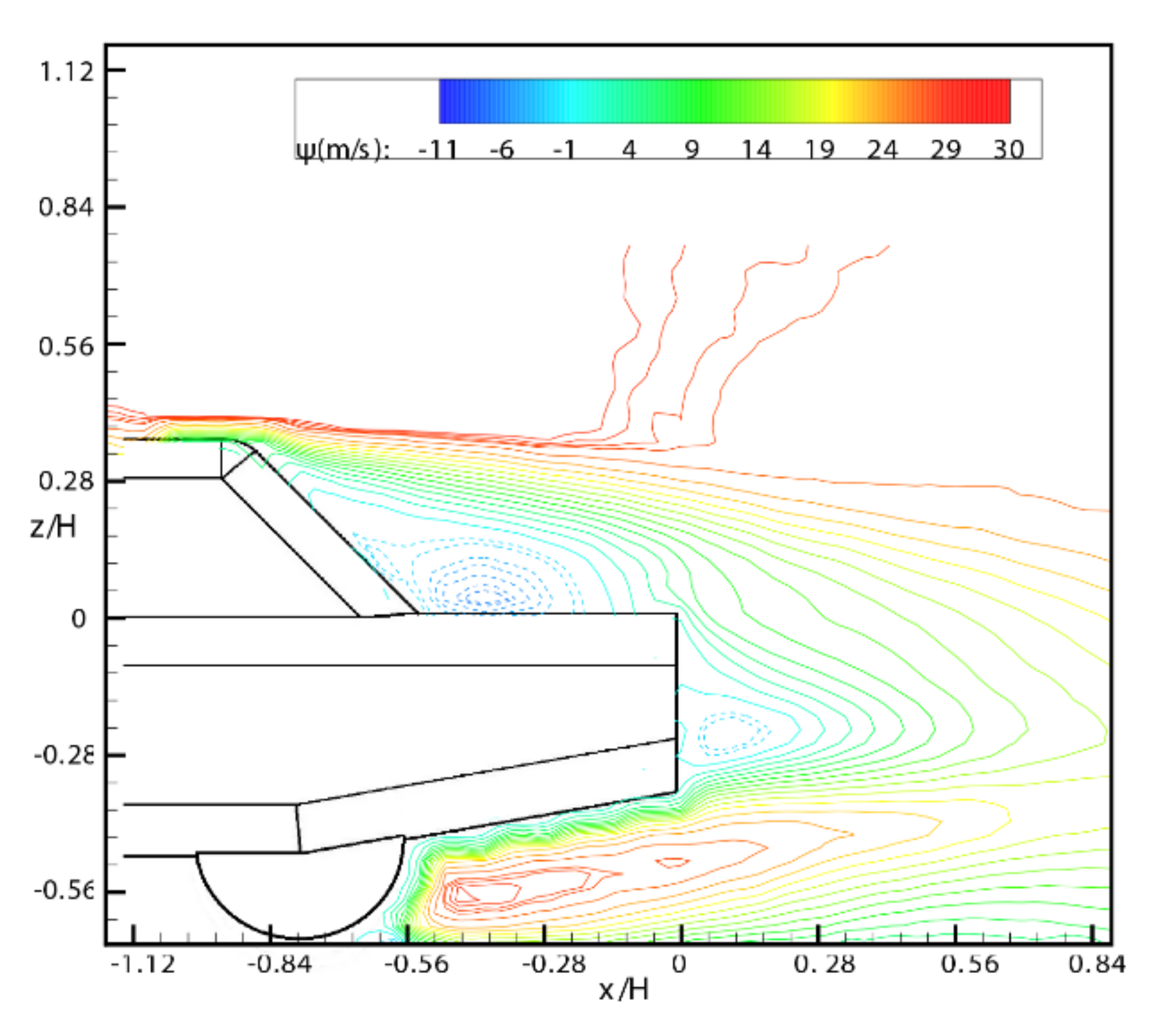
• There are two recirculation bubbles appearing behind the model tail due to the flow separation from the upper and the lower edges, referred to as vortices E and F, respectively. Additionally, the structure of vortex E resembles an L type, rather than the horseshoe type. The F vortex is composed of a row of alternating small vortices, which is characterized by a vortex with a rib structure in the vertical direction and a wave shape;
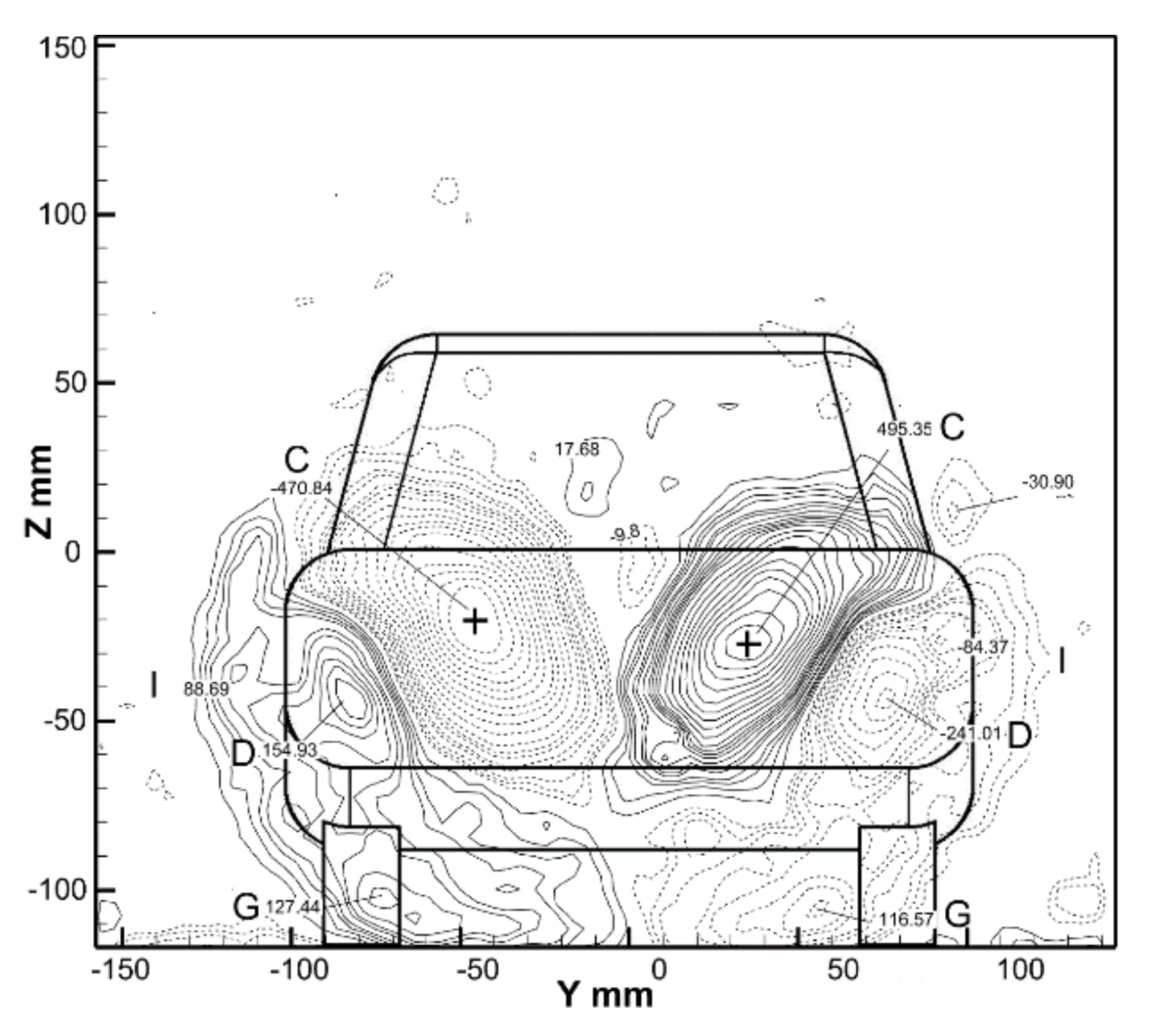
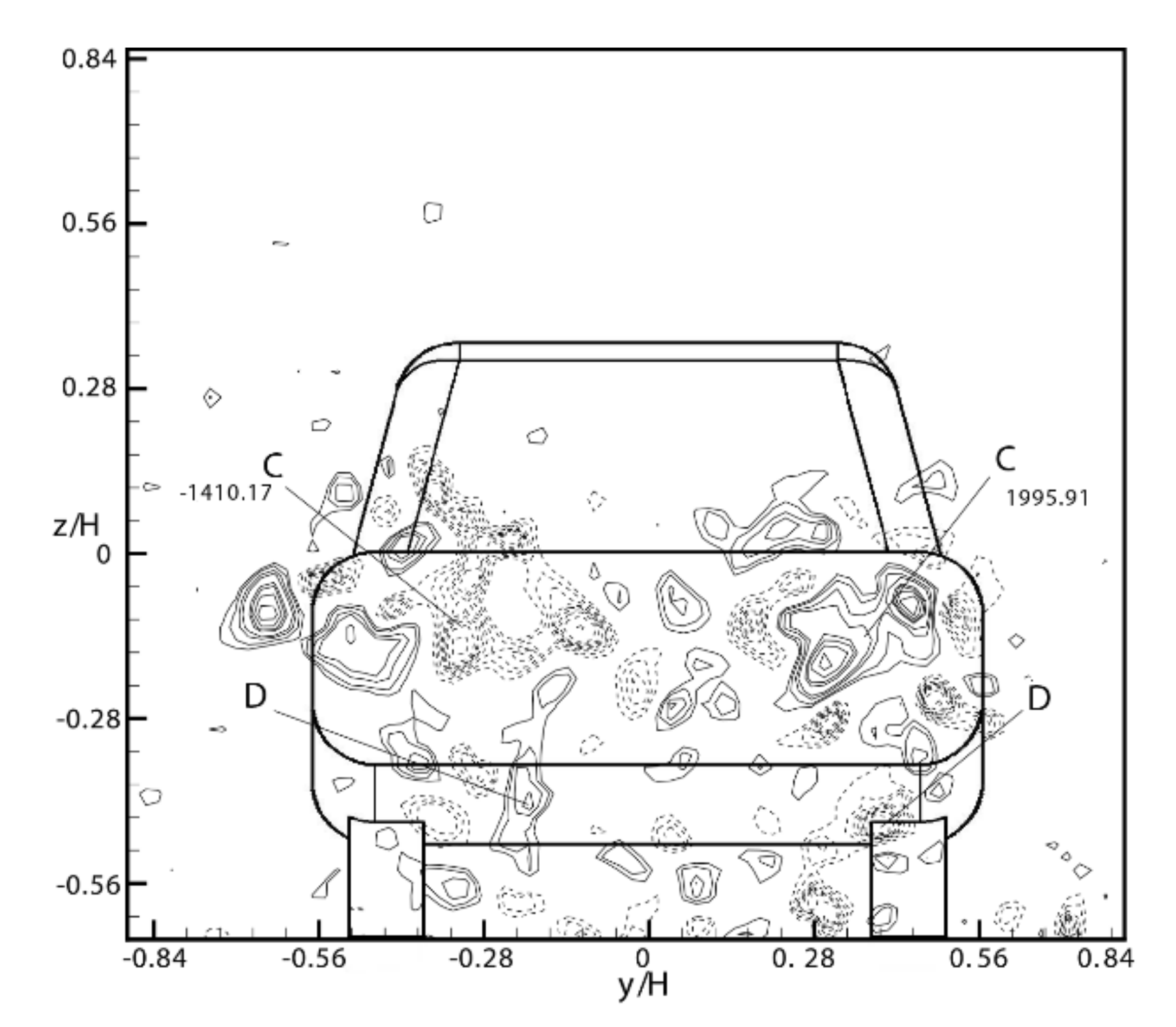
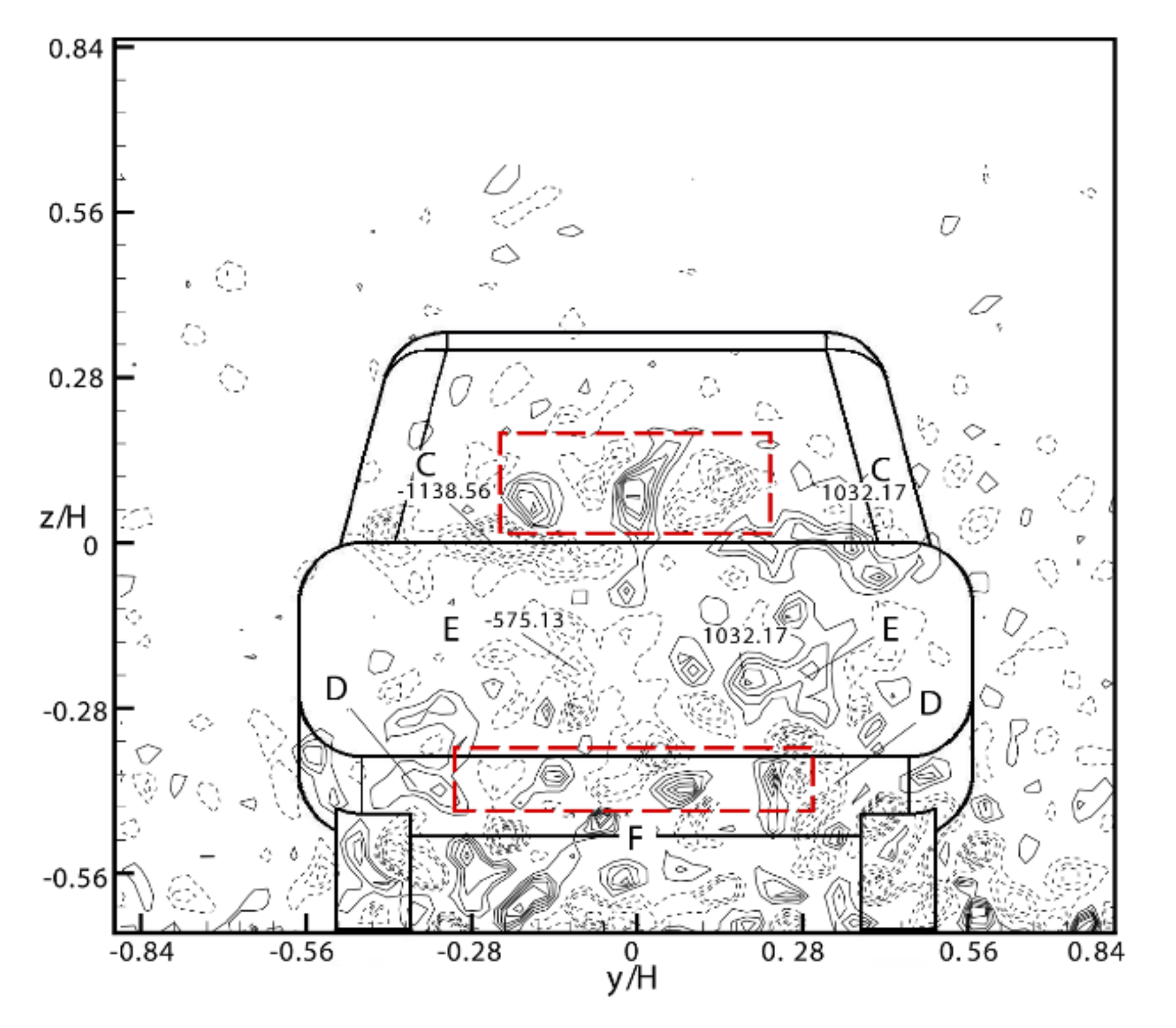
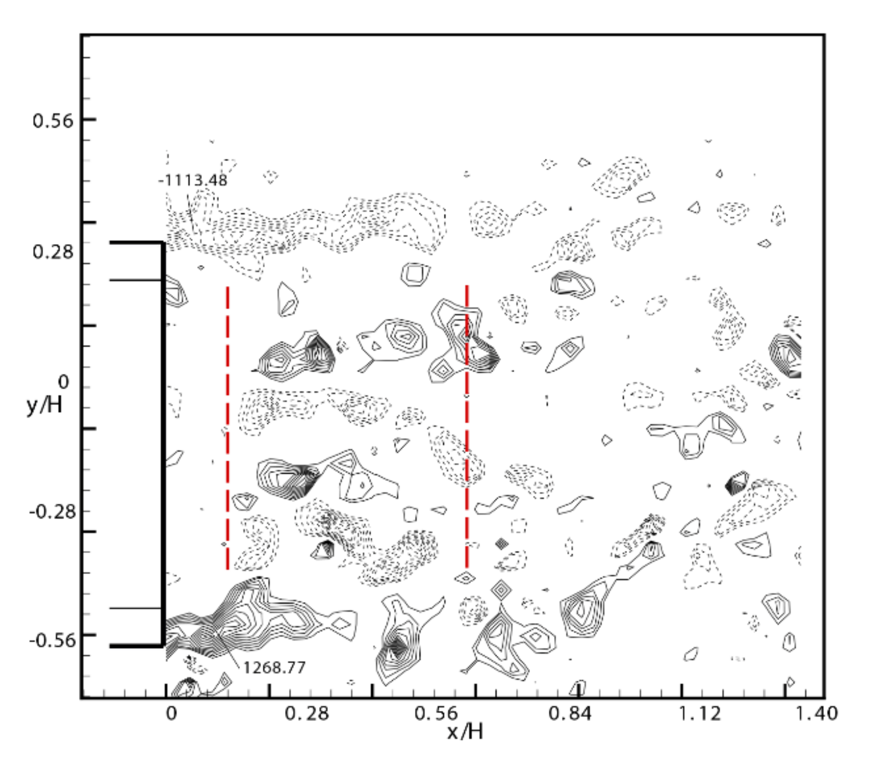
• Due to the upward angle of the tail of the MIRA model, a pair of predominant longitudinal 3D vortices similar to the C-pillar vortex, namely the D vortex, appears in the tail flow field structure. Additionally, C-pillar vortex contributes more energy than the D vortex. A pair of vertical separation vortices, namely I vortex, generates due to the airflow separation on both sides of the tail of the model;
• Between the ground and the model underside, due to the flow pressure difference between the inside gap and the outside, the shear layer eventually rolls up into a pair of longitudinal vortices Gt;
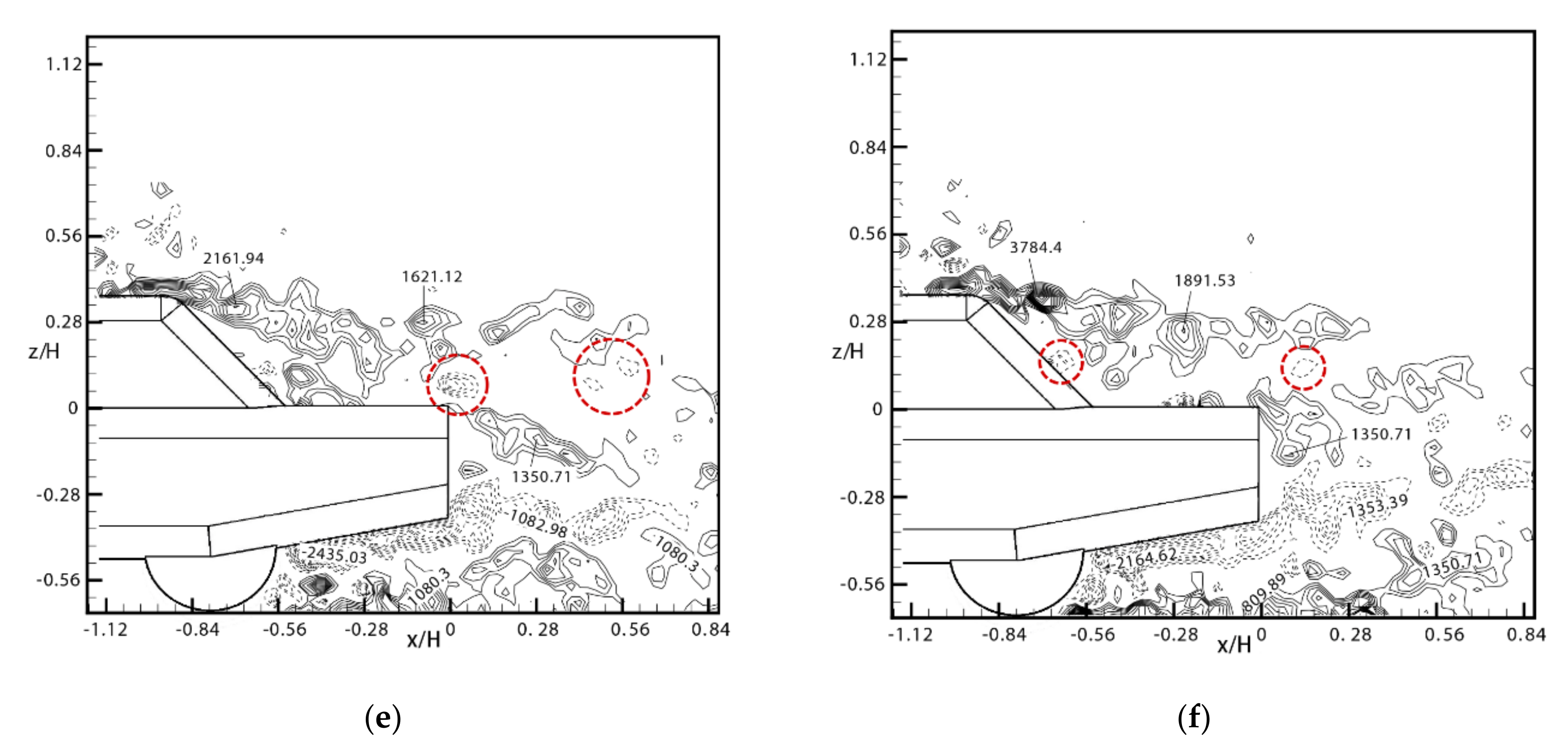
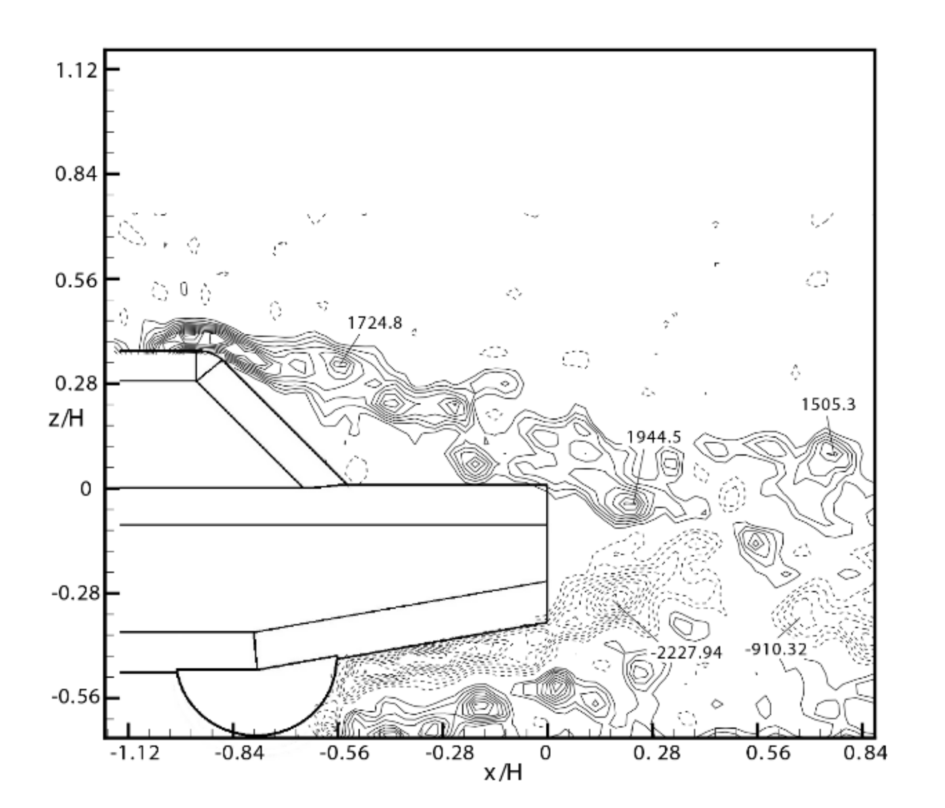
• The instantaneous flow shows a certain formation and shedding cycle of the hairpin vortex. It is deduced that a new vortex reproduces on the back window only after a vortex sheds from the deck lid.

In conclusion, this paper visually shows the flow structure of the MIRA notchback model and analyses the flow mechanism. It provides a reference for the development of automobile aerodynamic drag reduction, which is conducive to energy conservation.

References

1. Beaudoin, J.-F.; Aider, J.-L. Drag and lift reduction of a 3D bluff body using flaps. Exp. Fluids 2008, 44, 491–501. [Google Scholar] [CrossRef]
2. Tunay, T.; Sahin, B.; Akilli, H. Experimental and numerical studies of the flow around the Ahmed body. Wind. Struct. Int. J. 2013, 17, 515–535. [Google Scholar] [CrossRef]
3. Carr, G.W. Correlation of Pressure Measurements in Model and Full-Scale Wind Tunnels and on the Road; SAE Technical Paper Series; SAE International: Warrendale, PA, USA, 1975; Volume 84, pp. 365–379. [Google Scholar]
4. Nouzawa, T.; Haruna, S.; Hiasa, K.; Nakamura, T.; Sato, H. Analysis of Wake Pattern for Reducing Aerodynamic Drag of Notchback Model; SAE Technical Paper Series; SAE International: Warrendale, PA, USA, 1990; Volume 99, pp. 486–494. [Google Scholar]
5. Nouzawa, T.; Hiasa, K.; Nakamura, T.; Kawamoto, A.; Sato, H. Unsteady-Wake Analysis of Aerodynamic Drag of a Notchback Model with Critical Afterbody Geometry; SAE Technical Paper Series; International Congress & Exposition: Amsterdam, The Netherlands, 1992. [Google Scholar]
6. Hucho, W.H. Aerodynamics of Road Vehicle from Fluid Mechanics to Vehicle. Engineering, 4th ed.; Butterworth-Heinemann: Oxford, UK, 1987. [Google Scholar]
7. Jenkins, L.N. An Experimental Investigation of the Flow Over the Rear End of a Notchback Automobile Configuration; SAE Technical Paper Series; SAE International: Warrendale, PA, USA, 2000; Volume 109, pp. 477–496. [Google Scholar]
8. Gilhome, B.R.; Saunders, J.W.; Sheridan, J. Time Averaged and Unsteady Near-Wake Analysis of Cars; SAE Technical Paper; SAE International: Warrendale, PA, USA, 2001; Volume 110, pp. 1179–1196. [Google Scholar]
9. Okada, Y.; Nouzawa, T.; Nakamura, T.; Okamoto, S. Flow structures above the trunk deck of sedan-type vehicles and their influence on high-speed vehicle stability 1st report: On-road and wind tunnel studies on unsteady flow characteristics that stabilize vehicle behavior. SAE Int. J. Passeng. Cars Mech. Syst. 2009, 2, 138–156. [Google Scholar] [CrossRef]
10. Bonitz, S.; Larsson, L.; Lofdahl, L.; Broniewicz, A. Structures of Flow Separation on a Passenger Car. SAE Int. J. Passeng. Cars Mech. Syst. 2015, 8, 177–185. [Google Scholar] [CrossRef] [Green Version]
11. Cadot, O.; Courbois, A.; Ricot, D.; Ruiz, T.; Harambat, F.; Herbert, V.; Vigneron, R.; Délery, J. Characterisations of force and pressure fluctuations of real vehicles. Int. J. Eng. Syst. Model. Simul. 2016, 8, 99. [Google Scholar] [CrossRef]
12. Wieser, D.; Nayeri, C.N.; Paschereit, C.O. Wake Structures and Surface Patterns of the DrivAer Notchback Car Model under Side Wind Conditions. Energies 2020, 13, 320. [Google Scholar] [CrossRef] [Green Version]
13. Palaskar, P.M. Effect of Side Taper on Aerodynamics Drag of a Simple Body Shape with Diffuser and without Diffuser. SAE Technical Paper 2016-01-1621. 2016. Available online: https://www.sae.org/publications/technical-papers/content/2016-01-1621/ (accessed on 28 July 2021).
14. Bearman, P. Near wake flows behind two- and three-dimensional bluff bodies. J. Wind. Eng. Ind. Aerodyn. 1997, 69–71, 33–54. [Google Scholar] [CrossRef]
15. Liu, K.; Zhang, B.; Zhang, Y.; Zhou, Y. Flow structure around a low-drag Ahmed body. J. Fluid Mech. 2021, 913, A21. [Google Scholar] [CrossRef]
16. Lawson, N.J.; Garry, K.P.; Faucompret, N. An investigation of the flow characteristics in the bootdeck region of a scale model notchback saloon vehicle. Part D J. Automob. Eng. 2007, 221, 739–754. [Google Scholar] [CrossRef] [Green Version]
17. Wang, X.W.; Zhou, Y.; Pin, Y.F.; Chan, T.L. Turbulent near wake of an Ahmed vehicle model. Exp. Fluids 2013, 54, 1–19. [Google Scholar] [CrossRef]
18. Cenedese, A.; Doglia, G.; Sallusti, M.; Viotti, P. PIV velocity measurements close to a bluff body. J. Wind. Eng. Ind. Aerodyn. 1993, 50, 383–392. [Google Scholar] [CrossRef]
19. Goh, E.K. An Experimental Study into the Time-Dependent Characteristics of a Road Vehicle Wake Flow. Ph.D. Thesis, Department of Aeronautics, Imperial College, London, UK, 1994. [Google Scholar]
20. Ahmed, S.R.; Ramm, G.; Faltin, G. Some Salient Features of the Time-Averaged ground Vehicle Wake; SAE Transactions: Warrendale, PA, USA, 1984. [Google Scholar]
Figure 1. (a) Original size of MIRA notch back model; (b) 1/8 scale test mode in wind tunnel.
Energies 14 04568 g001
Figure 2. PIV measurements in three orthogonal planes: (a) y–z planes; (b) x–z planes; and (c) x–y planes.
Energies 14 04568 g002aEnergies 14 04568 g002b
Figure 3. Different plane locations in three orthogonal planes: (a) Longitudinal planes; (b) Spanwise planes; and (c) Transverse planes.
Energies 14 04568 g003
Figure 4. Iso-contours of time-averaged streamwise vorticity, ωx in the y–z plane at x/H = −0.7. Minimum and incremental values of vorticity are ωx,min = −45.221 s−1, 27.221 s−1, and Δωx = 20.430 s−1, respectively.
Energies 14 04568 g004
Figure 5. Iso-contours of time-averaged stream-wise vorticity, ωx in the y–z plane at x/H = −0.39. Minimum and incremental values of vorticity are ωx,min = −46.747 s−1, 48.778 s−1, and Δωx = 28.748 s−1, respectively.
Energies 14 04568 g005
Figure 6. Iso-contours of time-averaged streamwise vorticity, ωx in the y–z plane at x/H = −0.11. Minimum and incremental values of vorticity are ωx,min = −45.178 s−1, 50.476 s−1, and Δωx = 59.102 s−1, respectively.
Energies 14 04568 g006
Figure 7. Iso-contours of time-averaged stream-wise vorticity, ωx in the y–z plane at x/H = 0.28. Minimum and incremental values of vorticity are ωx,min = −65.067 s−1, 56.812 s−1, and Δωx = 91.841 s−1, respectively.
Energies 14 04568 g007
Figure 8. Iso-contours of time-averaged stream-wise vorticity, ωx in the y–z plane at x/H = 0.67. Minimum and incremental values of vorticity are ωx,min = −9.804 s−1, 17.676 s−1, and Δωx = 24.774 s−1, respectively.
Energies 14 04568 g008
Figure 9. Schematic of vortex E with “L” type.
Energies 14 04568 g009
Figure 10. Iso-contours of instantaneous stream-wise vorticity, ωx in the y–z plane at x/H = −0.7. Minimum and incremental values of vorticity are ωx,min = −185.343 s−1, 215.220 s−1, and Δωx = 143.058 s−1, respectively.
Energies 14 04568 g010
Figure 11. Iso-contours of instantaneous stream-wise vorticity, ωx in the y–z plane at x/H = −0.39. Minimum and incremental values of vorticity are ωx,min = −347.552 s−1, 370.918 s−1, and Δωx = 128.298 s−1, respectively.
Energies 14 04568 g011
Figure 12. Schematic of the separated spanwise roll wrapped with the rib structure. (a) spanwise roll with the rib structure occurring at the upper edge of the back window; (b) spanwise roll with the rib structure occurring on the lower edge of the model rear.
Energies 14 04568 g012
Figure 13. Iso-contours of instantaneous streamwise vorticity ωx in y–z plane at x/H = −0.11. Minimum and incremental values of vorticity are ωx,min = −251.859 s−1, 257.007 s−1, and Δωx = 141.352 s−1, respectively.
Energies 14 04568 g013
Figure 14. Iso-contours of instantaneous streamwise vorticity ωx in y–z plane at x/H = 0.28. Minimum and incremental values of vorticity are ωx,min = −230.944 s−1, 280.708 s−1, and Δωx = 225.428 s−1, respectively.
Energies 14 04568 g014
Figure 15. Iso-contours of instantaneous streamwise vorticity ωx in the y–z plane at x/H = 0.67. Minimum and incremental values of vorticity are ωx,min = −406.435 s−1, 284.304 s−1, and Δωx = 236.474 s−1, respectively.
Energies 14 04568 g015
Figure 16. Iso-contours of time-averaged streamwise vorticity ω in x–z plane at y/H = 0. Minimum and incremental values of vorticity are ωy,min = −179.091 s−1, 337.075 s−1, and Δωy = 143.379 s−1, respectively.
Energies 14 04568 g016
Figure 17. Iso-contours of time-averaged streamwise vorticity ωy in x–z plane at y/H = 0.28. Minimum and incremental values of vorticity are ωy,min = −263.339 s−1, 503.642 s−1, and Δωy = 188.227 s−1, respectively.
Energies 14 04568 g017
Figure 18. Time-averaged velocity streamline in x–z plane at y/H = 0, colored with velocity magnitude (Vel Mag, m/s).
Energies 14 04568 g018
Figure 19. Iso-contours of t time-averaged streamwise velocity in x–z plane at y/H = 0.
Energies 14 04568 g019
Figure 20. The hairpin vortex shedding sequence at y/H = 0. Minimum and incremental values of vorticity are ωy,min = −542.159 s−1, 539.48 s−1, and Δωy = 300.455 s−1, respectively. (af) shows the certain formation and shedding cycle of the hairpin vortex.
Energies 14 04568 g020aEnergies 14 04568 g020b
Figure 21. Iso-contours of instantaneous streamwise vorticity, ωy in x–z plane at y/H = 0.28. Minimum and incremental values of vorticity are ωy,min = −251.519 s−1, 407.288 s−1 and Δωy = 235.288 s−1, respectively.
Energies 14 04568 g021
Figure 22. Iso-contours of instantaneous streamwise vorticity, ωz in x–y plane at z/H = 0.18. Minimum and incremental values of vorticity are ωz,min = −405.572 s−1, 329.056 s−1, and Δωz = 169.530 s−1, respectively.
Energies 14 04568 g022
Figure 23. Iso-contours of instantaneous streamwise vorticity, ωz in x–y plane at z/H = −0.08. Minimum and incremental values of vorticity are ωz,min = −478.213 s−1, 474.689 s−1, and Δωz = 190.581 s−1, respectively.
Energies 14 04568 g023
Figure 24. Iso-contours of instantaneous streamwise vorticity ωz in x–y plane at z/H = −0.19. Minimum and incremental values of vorticity are ωz,min = −650.890 s−1, 449.812 s−1, and Δω = 253.948 s−1, respectively.
Energies 14 04568 g024
Figure 25. Iso-contours of time-averaged streamwise vorticity, ωz in the x–y plane at z/H = 0.18. Minimum and incremental values of vorticity are ωz,min = −66.086 s−1, 69.512 s−1, and Δωz = 79.165 s−1, respectively.
Energies 14 04568 g025
Figure 26. Iso-contours of time-averaged streamwise vorticity, ωz in the x–y plane at z/H = −0.08. Minimum and incremental values of vorticity are ωz,min = −119.654 s−1, 132.170 s−1, and Δωz = 96.175 s−1, respectively.
Energies 14 04568 g026
Figure 27. Iso-contours of averaged streamwise vorticity, ωz in x–y plane at z/H = −0.19. Minimum and incremental values of vorticity are ωz,min = −100.539 s−1, 98.948 s−1, and Δωz = 117.932 s−1, respectively.
Energies 14 04568 g027
Figure 28. Iso-contours of averaged stream- wise vorticity, ωz in x–y plane at z/H = −0.34. Minimum and incremental values of vorticity are ωz,min = −103.715 s−1, 119.761 s−1, and Δωz = 58.150 s−1, respectively.
Energies 14 04568 g028
Figure 29. Flow structure schematic of MIRA notchback model.
Energies 14 04568 g029
Publisher’s Note: MDPI stays neutral with regard to jurisdictional claims in published maps and institutional affiliations.