Article

Comparison of 3D Solid and Beam–Spring FE Modeling Approaches in the Evaluation of Buried Pipeline Behavior at a Strike-Slip Fault Crossing

Graduate School of Engineering, Kyoto University, Kyoto 615-8530, Japan
*
Author to whom correspondence should be addressed.
Energies 2021, 14(15), 4539; https://doi.org/10.3390/en14154539
Submission received: 1 June 2021 / Revised: 29 June 2021 / Accepted: 8 July 2021 / Published: 27 July 2021
(This article belongs to the Special Issue Trenchless Construction Methods for Energy Pipelines)

Abstract

:
Validated 3D solid finite element (FE) models offer an accurate performance of buried pipelines at earthquake faults. However, it is common to use a beam–spring model for the design of buried pipelines, and all the design guidelines are fitted to this modeling approach. Therefore, this study has focused on (1) the improvement of modeling techniques in the beam–spring FE modeling approach for the reproduction of the realistic performance of buried pipelines, and (2) the determination of an appropriate damage criterion for buried pipelines in beam–spring FE models. For this paper, after the verification of FE models by pull-out and lateral sliding tests, buried pipeline performance was evaluated at a strike-slip fault crossing using nonlinear beam–spring FE models and nonlinear 3D solid FE models. Material nonlinearity, contact nonlinearity, and geometrical nonlinearity effects were considered in all analyses. Based on the results, pressure and shear forces caused by fault movement and pipeline deformation around the high curvature zone cause local confinement of the soil, and soil stiffness around the high curvature zone locally increases. This increases the soil–pipe interaction forces on pipelines in high curvature zones. The beam–spring models and design guidelines, because of the uniform assumption of the soil spring stiffness along the pipe, do not consider this phenomenon. Therefore, to prevent the underestimation of forces on the pipeline, it is recommended to consider local increases in soil spring stiffness around the high curvature zone in beam–spring models. Moreover, drastic increases in the strain responses of the pipeline in the beam–spring model is a good criterion for a damage evaluation of the pipeline.

1. Introduction

The pipeline network has been spread all over the world to provide the essential needs of human societies (e.g., for transmission of gas, water, oil, wastewater, and chemical products). Hence, there are a great deal of pipelines crossing seismic hazardous areas, such as high curvature zones [1]. Earthquakes are the greatest threat to structures [2]. In the case of buried pipelines, most damage arises due to permanent ground deformation (PDG), for example, fault dislocations, liquefaction, and landslides. However, small regions within the pipeline network and earthquake fault zones are prone to PGD; because they cause large deformation of the pipelines, the damage potential is very high. On the other hand, there are very few pipeline cases that are damaged by wave propagations [3,4]. Accordingly, this paper has focused on the stability analysis of buried pipelines subjected to the strike-slip fault movement during PGD. Earthquake fault movements cause plastic deformation and even rupture to buried pipelines. The damage of buried pipelines due to previous earthquakes has been reported and has caused severe health and environmental issues [5,6,7,8,9,10,11,12,13,14,15,16]. Damage to the pipeline system not only affects urban infrastructures’ serviceability after earthquakes, but also, owing to the leakage of ecologically dangerous materials (e.g., chemicals, natural gas, fuel, or liquid waste), they can result in health and environmental issues [17]. Therefore, it is essential to develop analysis methods for buried pipelines to ensure the reliable resistance and economic design of these pipelines. Remarkably, because PGD can cause severe pipeline damage, the construction of buried pipelines at earthquake fault intersections is a key problem in engineering design tasks [1,18]. The effect of active fault crossings on buried pipelines has been investigated through several experimental studies [19,20]. Palmer et al. [21] described a large-scale testing facility at Cornell University and its working principles. O’Rourke and Bonneau [22] then performed large-scale tests to evaluate the effects of ground rupture on high-density polyethylene (HDPE) pipelines and the performance of steel gas pipelines distributed with 90° elbows. Lin et al. [23] performed small-scale tests to analyze the performance of buried pipelines under strike-slip faults. For the first time, the centrifuge-based approach was proposed by O’Rourke et al. [20] to model the ground faulting effects on buried pipelines, and several centrifuge tests have been performed to investigate the response of buried HDPE pipeline subjected to faulting displacement [24,25,26,27].
In 1975, the first analytical research on buried pipelines at a fault crossing was conducted by Newmark and Hall [28]. They evaluated a simplified analytical pipeline model by assuming cable-like behavior for a pipeline in small displacement, which was later extended by Kennedy et al. [29,30]. In those studies, the bending stiffness of the buried pipeline at the high curvature zone was neglected, which caused an overestimation of the bending stress–strain and increased the axial forces. Wang and Yeh [31] developed Kennedy et al. [30] model to strike-slip fault crossings by the extension of a simplified pipeline bending stiffness in their calculation. Wang and Yeh included the lateral soil yielding and introduced four segments to the buried pipeline at a fault crossing by partitioning. Two segments were adjacent to the fault crossing (the “high curvature zone”), and two were farther from the high curvature zone. However, the soil yielding starting point and partitioning assumptions were not realistic. Karamitros et al. [32] developed a method for strike-slip faults, wherein the pipeline is partitioned into four segments that are analyzed based on the beam-on-elastic-foundation and elastic beam theories. After the analytical solution, the longitudinal soil–pipe interaction was determined in addition to the steel pipe material’s non-linearity using a bilinear stress–strain relationship. The Karamitros et al. [32] model was developed by Trifonov and Cherniy [33] for normal fault crossings. They removed the symmetry conditions and estimated the axial elongation. Karamitros et al. [34], with the same assumption, extended their study [32] to normal-slip faults; however, this model has the same shortcomings as their previous study [32]. In 2012, an analytical model based on the stability model of Trifonov and Cherniy [33], including the operational loads (internal pressure and temperature gradient), was developed for the stress–strain analysis of buried pipelines at a fault crossing by Trifonov and Cherniy [35]; however, their study had the same shortcomings as their previous governing differential equation [33]. In 2020 and 2021, Talebi and Kiyono [36,37] introduced a novel nonlinear governing equation that includes the longitudinal sliding behavior of a pipe within soil during large PGDs, lateral elastoplastic soil–pipe interaction springs, and longitudinal forces made by geometrical nonlinearity effects. They removed the unrealistic assumptions and remarkably increased the accuracy and application area of the analytical methods for the problem of buried pipelines at active strike-slip fault crossings.
The efficacy of FEM-based analysis to assess the behavior of a buried pipeline crossing an active fault has been proved in the literature. FEM has been used to evaluate the buried pipeline performance with the assessment of criteria such as local buckling, ovalization, and tensile damages [18,38,39,40,41]. Vazouras et al. [39] modeled a hybrid (shell and solid elements beside the equivalent springs) pipeline buried in solid soil. Liu et al. [40] modeled a buried pipeline at a reverse fault crossing using the FE commercial code ABAQUS, in which the pipe was modeled as shell elements and the soil–pipe interaction was modeled as non-linear soil springs. In their study, the pipe and the soil–pipe interaction were modeled as shell elements and as non-linear soil springs, respectively. Besides, they had an investigation on the buckling of buried pipelines influenced by the yield strength and strain hardening parameters. Demirci et al. [41] studied the behavior of a continuous buried pipeline subjected to a reverse fault motion through a new experimental centrifuge modeling of a pipeline crossing a reverse fault. Additionally, 3D FEM analyses were used for more detailed results. Literature reviews show that various modeling approaches, including beam, shell, hybrid I (beam+shell), and hybrid II (spring+shell) for a pipe and springs, and soil continuum solid elements for soil modeling have been employed to evaluate pipeline performance against fault movement.
A 3D FE (3D solid)-based analysis, the most detailed approach for modeling a pipeline at a high curvature zone, including the shell elements and solid elements to simulate the buried pipeline and surrounding soil, respectively, can provide the most realistic evaluation of buried pipeline performance, including the local buckling, ovalization, and tensile damages. Typically, the 3D solid model is used for research purposes, owing to the modeling complexity. The beam–spring model is a simplified FE modeling approach, which uses beam and spring elements to model the pipe and soil–pipe interactions, respectively. Although it is pretty common to use a beam–spring model for the design purpose of buried pipelines at a fault crossing and all the design guidelines are extended based on this modeling approach for the analysis of buried pipelines, there is a gap in the literature for a detailed comparison of the beam–spring model and the 3D solid model results (a 3D solid model has almost realistic results). This comparison provides helpful conclusions for the development of the beam–spring modeling approach and the improvement of buried pipeline design guidelines.
This paper intends to present a detailed comparison between a nonlinear beam–spring modeling approach and a nonlinear 3D solid modeling approach to evaluate the performance of buried pipelines at strike-slip fault crossings to improve the beam–spring modeling approach and pipe damage criteria in this approach. In this regard, firstly, to verify the validity of the longitudinal and lateral soil–pipe interaction of the 3D solid model, a pipe and soil box model of pull-out and lateral sliding tests, based on Vazouras et al. [39], was simulated. The 3D solid model calibrated based on Vazouras et al. [39] and highly verified the results reported in the literature. Force–displacement diagrams of the equivalent soil-pipe interaction springs in the longitudinal, lateral, and vertical directions were extracted by displacement control FE analyses. Secondly, FE-base beam-spring models for identical pull-out and lateral sliding tests in previous 3D-solid models were created, and soil–pipe interaction springs were created based on the 3D solid model results and the results of beam-spring models were verified against the 3D-solid models for pull-out and lateral sliding tests. Finally, a 3D solid and a beam–spring FE model with identical properties for the problem of a buried pipeline at a strike-slip fault crossing were created. The responses of the buried pipeline modeled by both modeling approaches were compared to evaluate the pipe performance in both modeling approaches, and to extract any requirements in the development of the beam–spring modeling approach, and the development of the damage parameters and criteria.

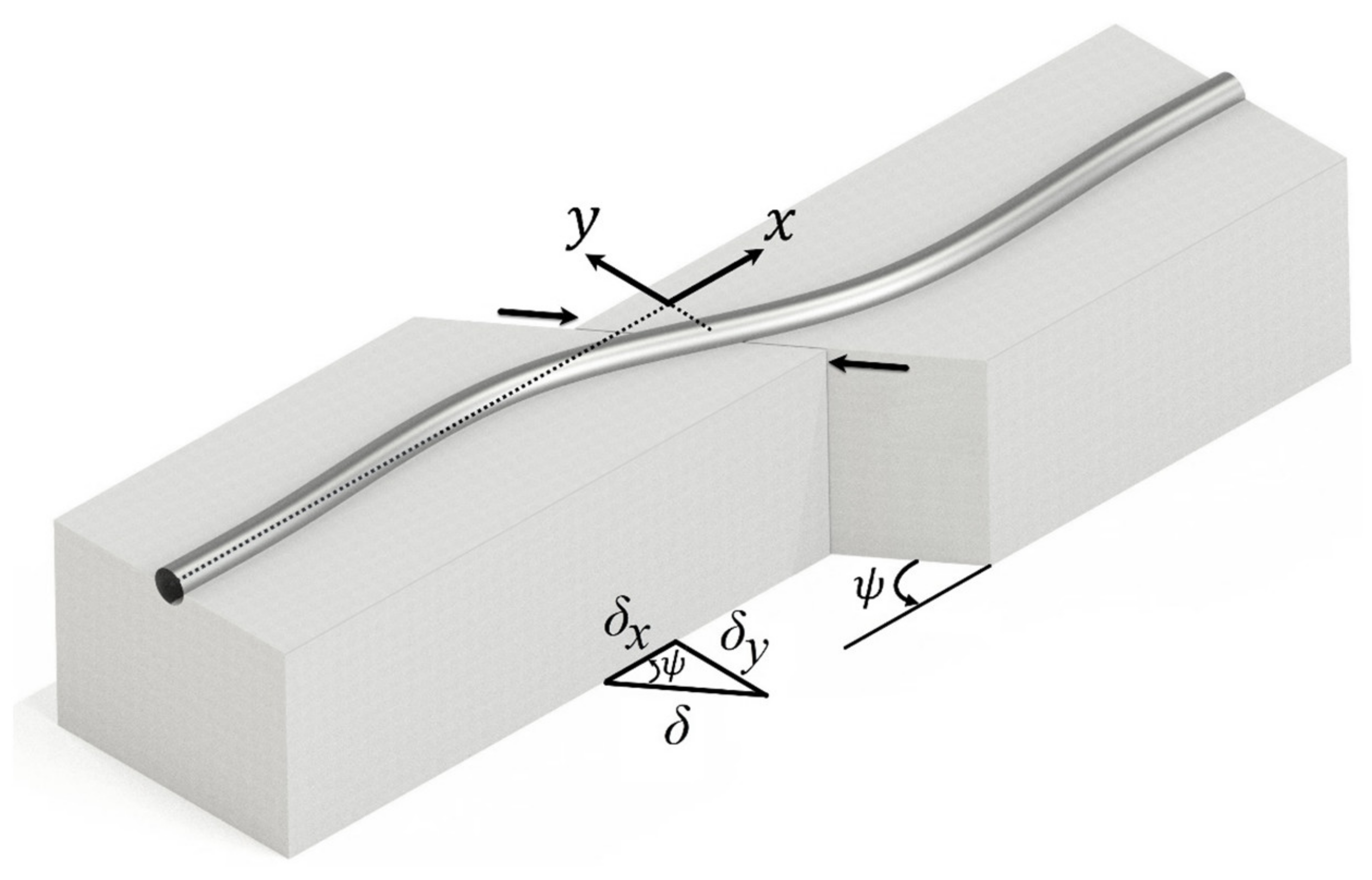
2. Analytical Evaluation of Buried Pipeline Behavior

Details of the strike-slip fault angle (ψ) and fault displacement (δ) are schematically shown in Figure 1, in which δx and δy are the longitudinal and lateral components of the fault displacement, respectively.
δx = δcosψ
δy = δsinψ
As mentioned in Section 1, Talebi and Kiyono [36,37] have extended the linear and nonlinear analytical methods for the stability analysis of buried pipelines at strike-slip faults with high accuracy results. Since, in this paper, the analytical method was just used for the parametric interpretation of the FE analyses results instead of the complex analytical approaches in the papers by [36,37], a simple linear analytical method mentioned by Talebi and Kiyono [42] was employed.
A simplified differential equilibrium equation for the pipeline crossing the strike-slip is expressed in Equation (1). By a closed-form solution, Equation (1) yields to Equation (4) [42].
E I d 4 w y d x 4 k t w y = 0
w y x = δ y 2 e β x c o s β x
where w y is the transverse displacement of the fault and β is
β = k t 4 E I 4  
In analytical methods, L c is the soil yielding zone at the high curvature zone of the pipeline. In fact, L c is the distance between the pipe–fault intersection point and the first point with zero deflection on the pipeline (shown in Figure 2).   L c is the first point after the fault line where deflection reaches zero. Based on Equation (4), where x = L c and w = 0 ,
L c π 2 4 E I k 4
Regarding Equation (6), the high curvature zone length ( L c ) has a direct relationship with EI and an inverse relationship with soil stiffness (k) [36].

3. Modeling Procedure

The comparison of buried pipeline performance at a strike-slip fault crossing using 3D solid and beam–spring FE modeling approaches was the main focus of the current study. Both the mentioned FEM modeling approaches were applied to investigate the problem of a buried pipeline at a strike-slip fault. The soil–pipe interaction modeling is the most complicated and important part of creating an FE model for the mentioned problem. Soil–pipe interaction modeling parameters can severely affect the pipe performance responses during faulting. Therefore, to have accurate models and results using both modeling approaches, in the first step, the soil–pipe interaction properties and modeling of the buried pipeline were validated using pull-out tests and lateral sliding test simulations. In the 3D solid model, the soil material model and contact properties are determinants for the calibration of the soil–pipe interaction. In the beam–spring model’s soil–pipe interaction, the spring properties are determinants. To validate the longitudinal soil–pipe interaction of the 3D solid FE model, three pull-out tests were simulated based on the model by Vazouras et al. [39] and the FE models’ results were verified against their results. Based on the 3D solid model’s pull-out tests, an identical beam–spring model was created, and its soil–pipe interaction results were verified against the 3D solid model. After verification of the 3D solid model soil–pipe interaction forces, three lateral sliding tests were created using the same 3D solid models, and lateral soil–pipe interaction forces were extracted. In the same manner, an identical beam–spring model for a lateral sliding test was created, and its lateral soil–pipe interaction forces were verified against the 3D solid model’s results. After calibration of the soil–pipe interaction parameters for the 3D solid and beam–spring models, we attempted to create FE models for the problem of a buried pipeline at a strike-slip fault crossing. All the FE models were created in the multi-purpose finite element program ABAQUS [43]. Both mentioned approaches include both geometrical and material nonlinearity effects.

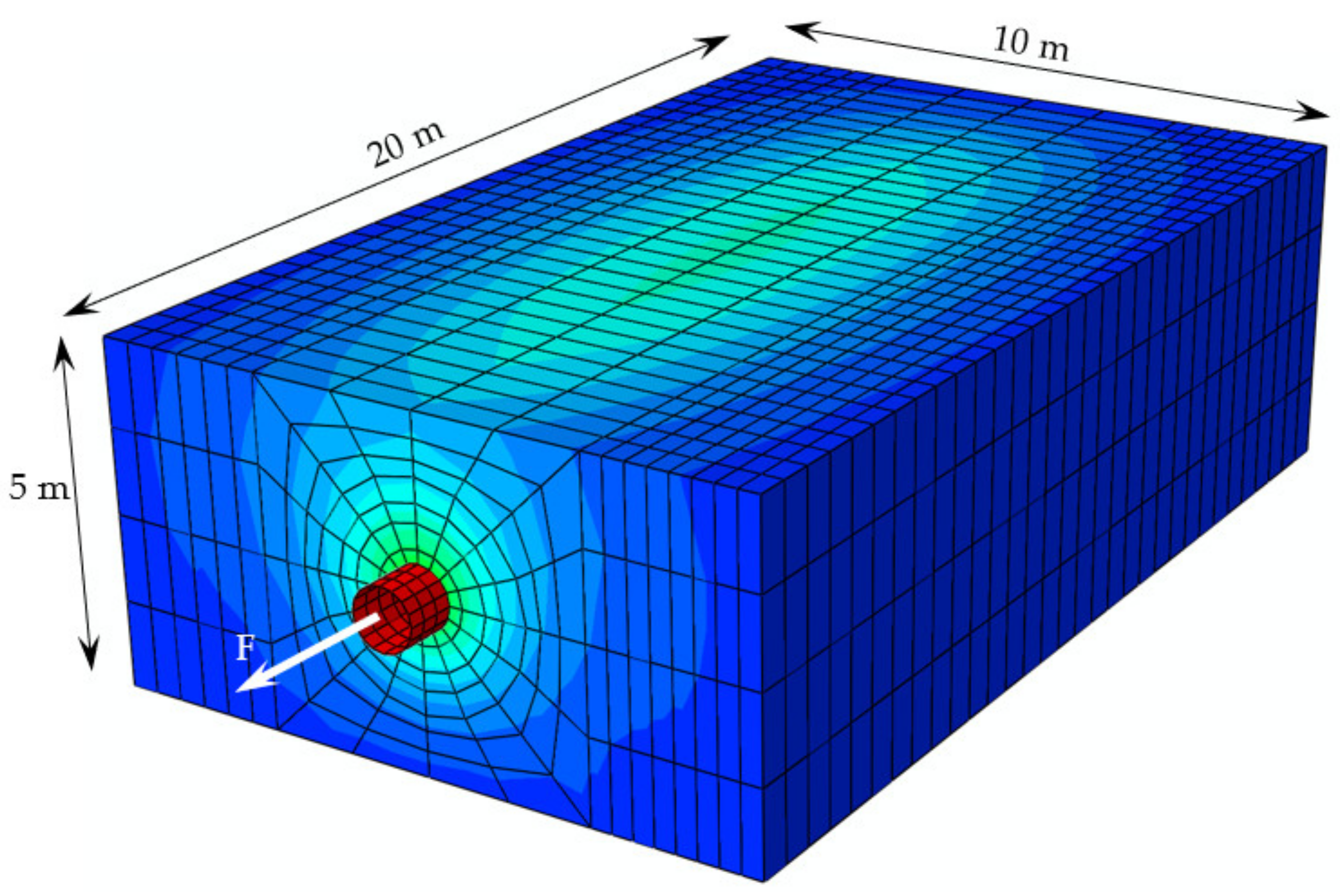
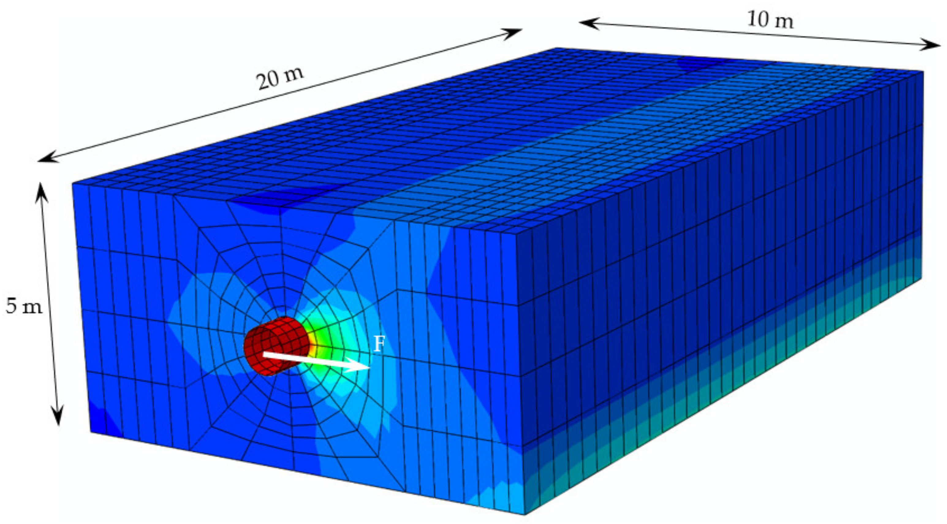
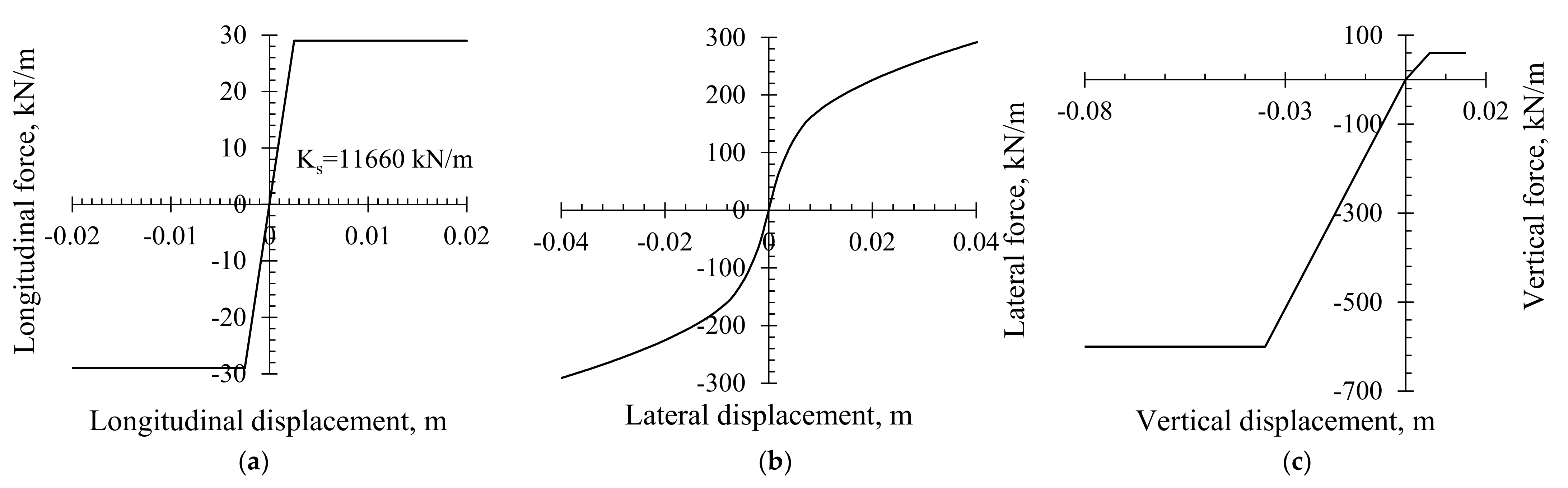
4. Longitudinal and Lateral Test Modeling

Two 3D FE models were created to study the longitudinal and lateral soil–pipe interaction and calibration of the 3D solid FE model soil–pipe interaction force–displacement relationship. The models were longitudinal pull-out and lateral sliding tests of the buried pipeline to show the force–displacement relationship of the longitudinal and lateral soil–pipe interaction, respectively. All the FE models were created in the multi-purpose finite element program ABAQUS [43].
Both the 3D solid and beam–spring models’ results were obtained for an X65 steel 36” pipeline with an outer diameter of 0.914 m, a thickness of 0.0095 m, Young’s modulus of 21 Tpa, a Poisson ratio of 0.3 , and a density of 7850 kg/m3. The Young’s modulus for pipe material was assumed to be 100 times stiffer than X65 steel for decreasing the pipeline deformation effect in the soil–pipe interaction evaluation. The pipeline was assumed to be buried in undrained clay. The soil had a density of 2000 kg/m3, a Young’s Modulus of 25 MPa, a Poisson ratio of 0.5 cohesion of 50 kPa, and a friction angle of 0°. As with real cases, it was assumed that the buried pipeline was surrounded by a thin layer of sand. Thus, a frictional soil–pipe interaction was employed. In addition, the soil box was modeled with the dimensions of 20 m × 10 m × 5 m. Table 1 reports the pipe and soil properties.
In the 3D solid model, the soil material was defined as an elastic–perfectly plastic Mohr–Coulomb constitutive model. The pipe elements were 4-node shell S4R element type, and the soil elements were 8-node linear brick, reduced integration C3D8R element type. The geometrical nonlinearity effect was taken into account for all analyses by the Nlgeom method, conducted by the FE program of ABAQUS.
In the beam–spring model, B31, RB3D2, and CONN3D2 elements were employed for the pipe elements, rigid bodies, and soil, respectively. The soil–pipe interaction was modeled through equivalent nonlinear soil springs in the longitudinal, lateral (horizontal), and vertical directions extracted from the 3D FE simulation results based on the pull-out and sliding tests. The Nlgeom method was the same as the 3D solid model’s and was implemented into the beam–spring model to have geometrical nonlinearity effects.

4.1. 3D FEM Analyses Results

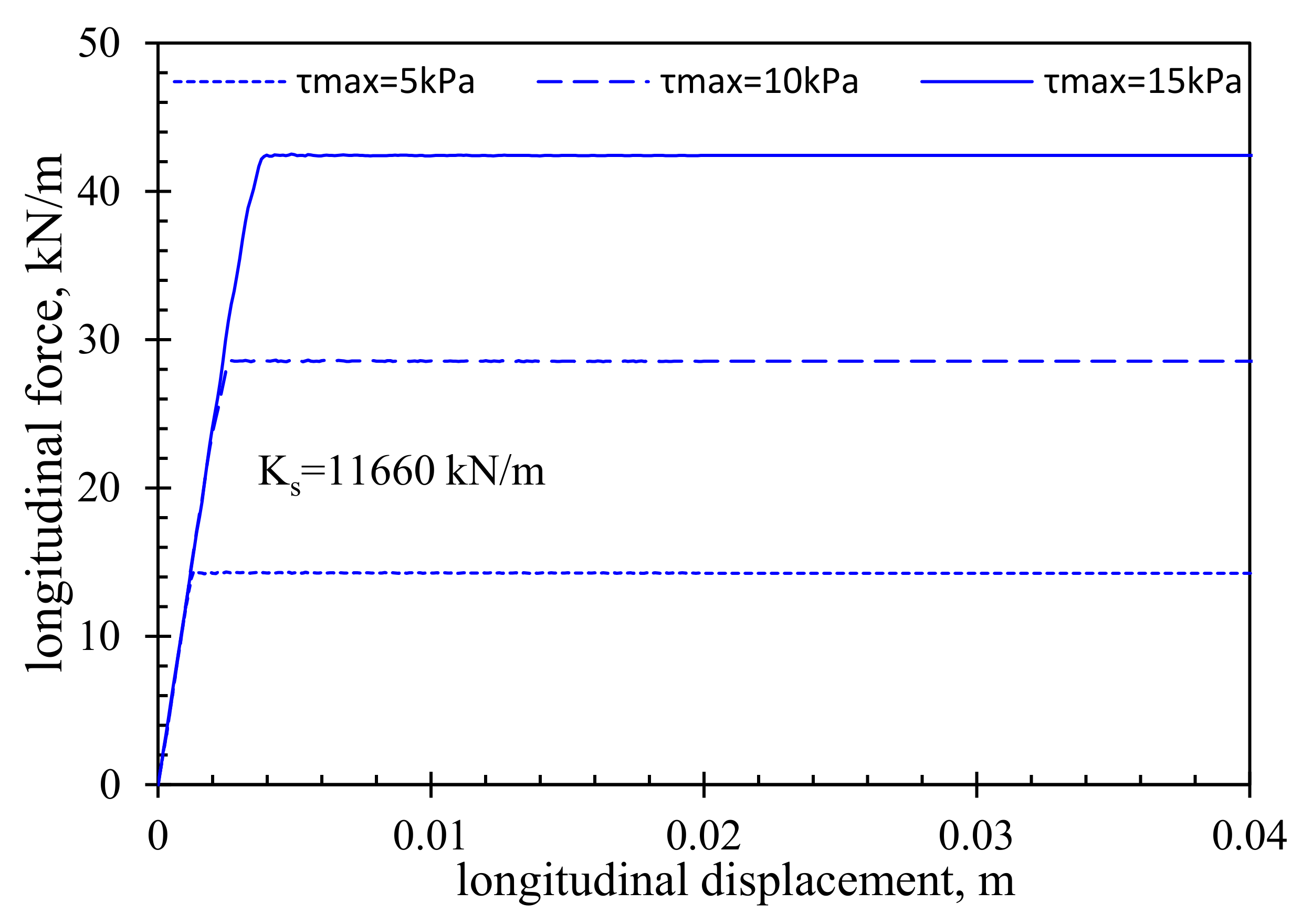
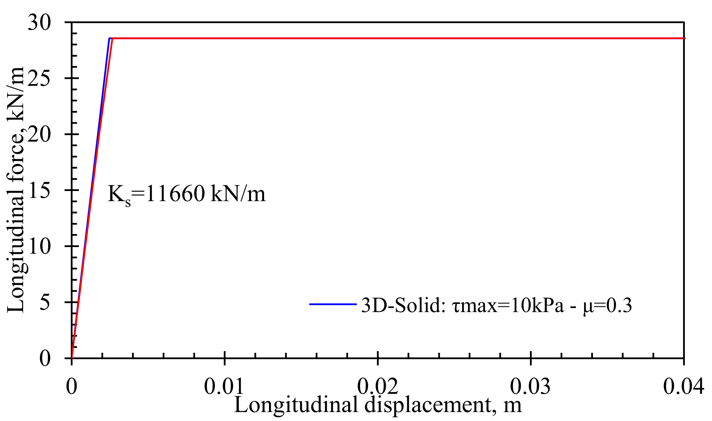
4.1.1. Longitudinal Pull-Out Test Analyses

As shown in Figure 3, three 3D solid FE cases for longitudinal pull-out tests were created to evaluate the longitudinal soil–pipe interaction. The FE analysis results were verified with the pull-out test results of Vazouras et al. [39] in Figure 4. As illustrated, good compatibility can be seen between the results of the current study and the results reported by Vazouras et al., 2015. Figure 5 shows the 3D solid models’ longitudinal force–displacement diagram of the unit length of the pipeline for the pull-out test results in the three cases with friction coefficients of 0.2, 0.3, and 0.4, in which the longitudinal soil–pipe interaction curves are elastic–perfectly plastic curves for all the cases. Therefore, the pipeline slides when the longitudinal force reaches the corresponding displacement of the yielding force in each case.
After verification of the 3D solid model for the pull-out test for the 0.2, 0.3, and 0.4 friction coefficient cases, the case with the 0.3 friction coefficient ( τ m a x = 10   kPa ) was selected as the main case for this paper.
To compare the beam–spring model versus the 3D solid model, it was required to create a FE model with identical properties and geometry and verify that their soil–pipe interaction behavior was almost identical. To achieve this goal, a beam–spring model with equivalent properties to a 3D solid pull-out test model ( μ = 0.3 and τ m a x = 10   kPa ) was created. The soil–pipe interaction spring in the beam–spring model was created based the on 3D solid force–displacement curve in Figure 5, and the modeling details of the beam–spring model are clarified in Section 4. As presented in Figure 6, the beam–spring model’s longitudinal soil–pipe interaction force–displacement curve is almost the same as the 3D solid model’s, and it was verified against the 3D solid model’s results.

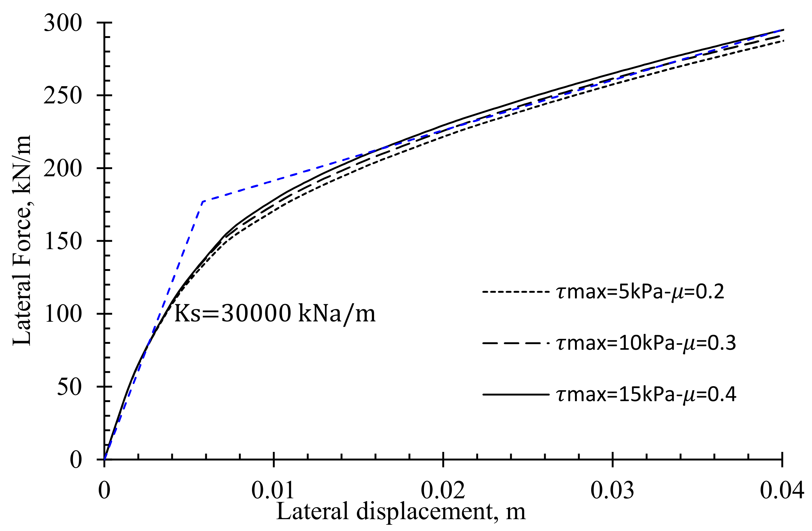
4.1.2. Lateral Sliding Test Analyses

After verification of the 3D solid model’s longitudinal soil–pipe interaction results, a 3D solid FE model with identical properties with the longitudinal pull-out 3D solid FE model was extended to simulate a lateral sliding test for the reproduction of the lateral soil–pipe interaction force–displacement relationship. The displacement contours for the lateral sliding test model are illustrated in Figure 7. Lateral soil–pipe interaction force–displacement curves for cases with friction coefficients of 0.2, 0.3, and 0.4 are shown in Figure 8. Based on Figure 8, all the cases with different friction coefficients have identical behavior in the elastic range and their discrepancy in a nonlinear range is almost negligible. In addition, it shows the soil material properties’ effect on the lateral soil–pipe interaction is predominant in comparison with the contact properties. On the contrary, based on Figure 5, the contact properties have a higher impact on the longitudinal soil–pipe interaction force–displacement relationship in comparison with the soil material.
The lateral soil–pipe interaction spring properties of the verified beam–spring model in the pull-out test were extended based on the 3D solid lateral sliding test model results for the μ = 0.3 and τ m a x = 10   kPa case. As shown in Figure 9, the lateral soil–pipe interaction force–displacement curve of the beam–spring model in the lateral sliding test is almost the same as the 3D solid model’s for the same case. Therefore, the beam–spring lateral soil–pipe interaction is verified to have almost identical behavior with the 3D solid model in the case with μ = 0.3 and τ m a x = 10   kPa .

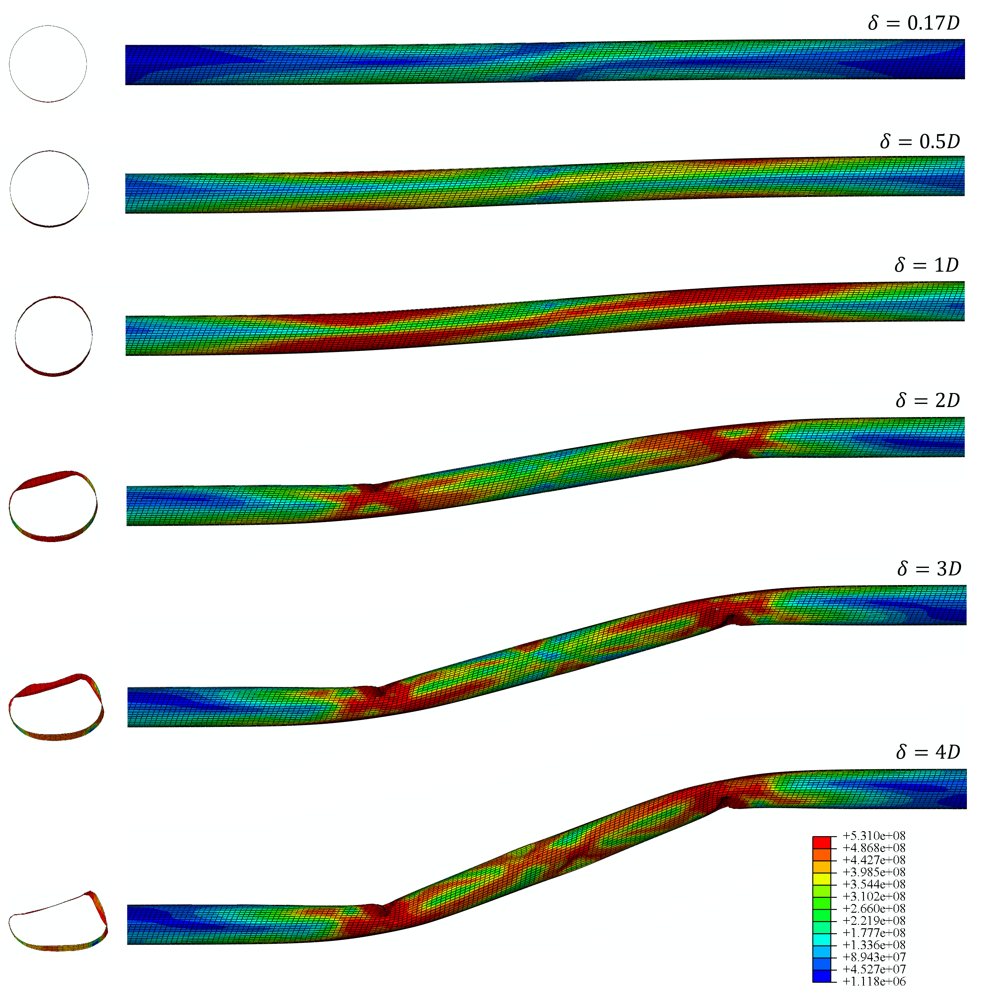
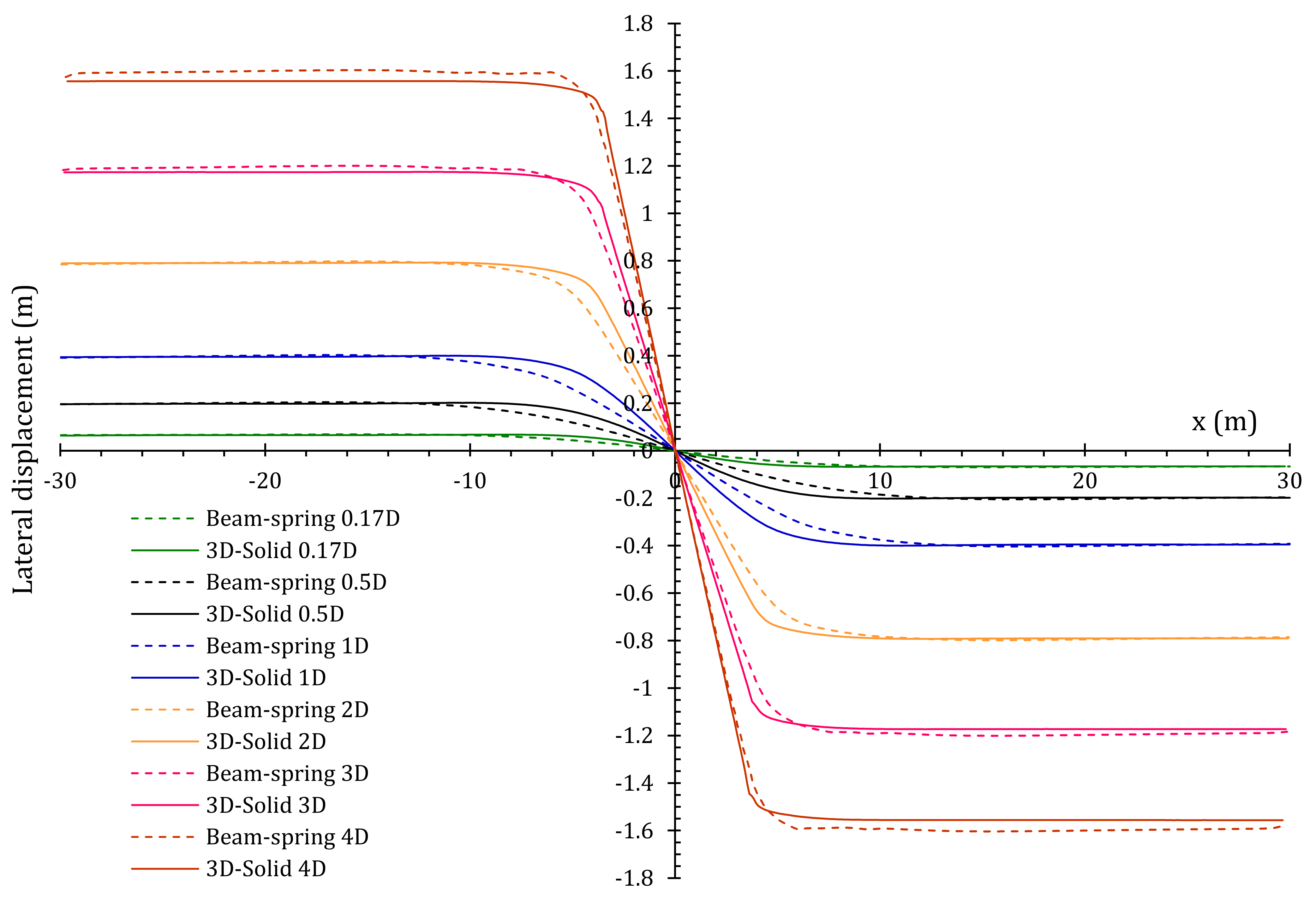
5. Modeling and Analysis Results of a Pipeline at a Strike-Slip Fault Crossing
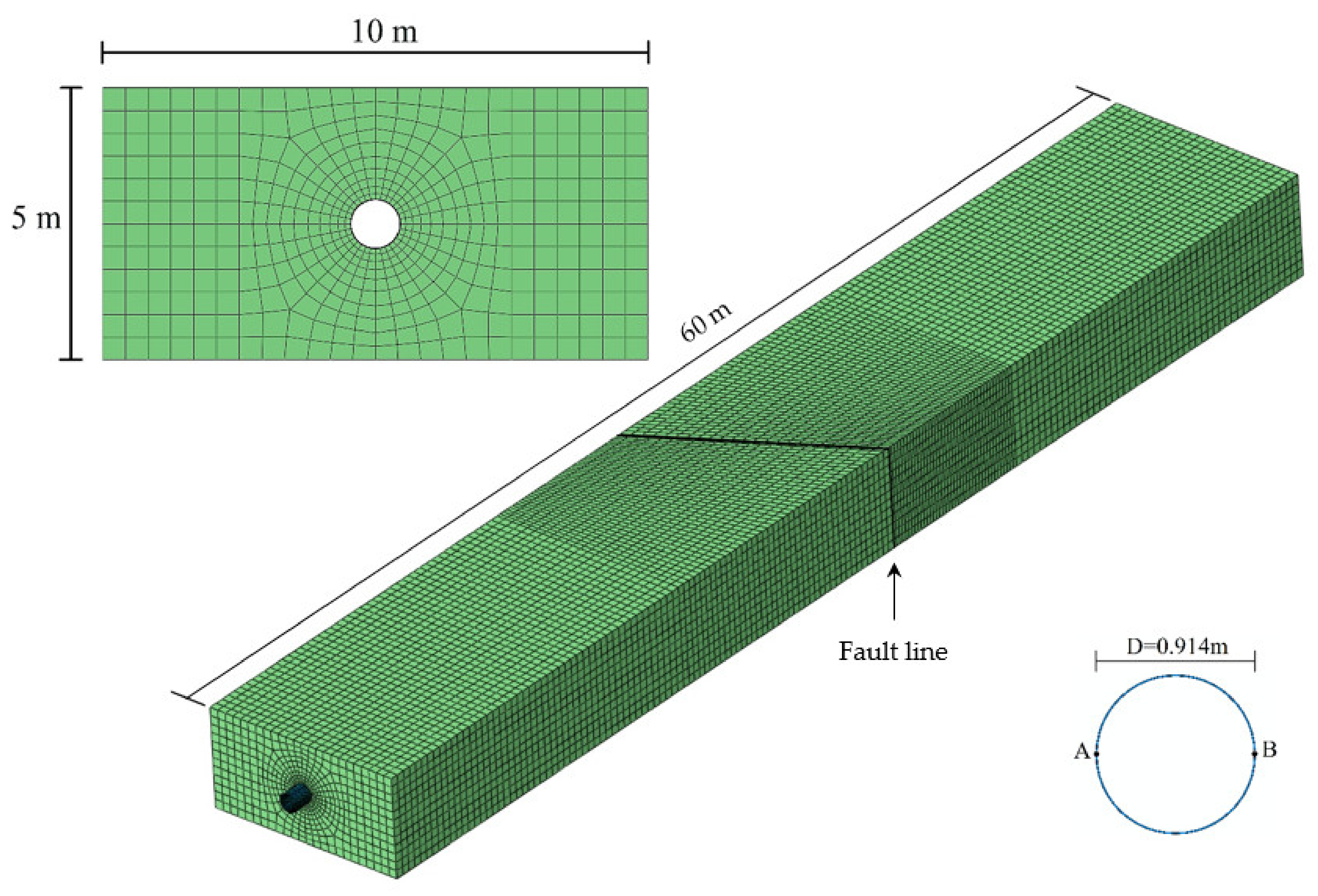
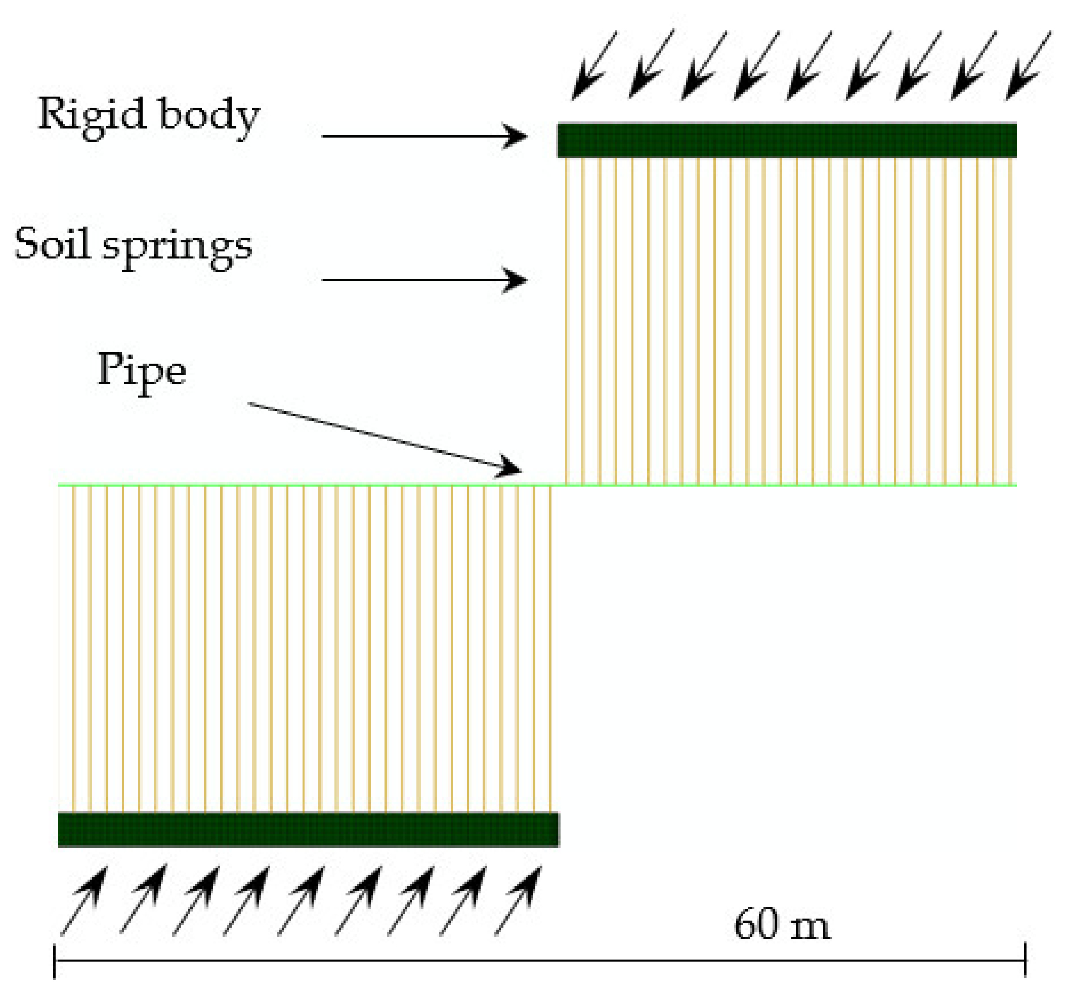
5.1. FE Modeling

Both the verified 3D solid and verified beam–spring models were extended for the problem of a buried steel pipeline subjected to a 60° strike-slip fault movement, based on the verified pull-out test and lateral sliding test models. In addition, both the 3D solid and the beam–spring modeling properties for the soil, pipe, springs, and contacts were identical with the FE models for the pull-out and sliding tests (except the pipe material properties). The soil box dimensions were 60 m × 10 m × 5 m; the 3D solid model is shown in Figure 10, and the beam–spring model is shown in Figure 11. A friction coefficient of 0.3 was assumed for contact modeling, which is equivalent to the demonstrated soil with a maximum shear stress equal to 10 kPa. The fault movements and boundary conditions were also applied to the soil box’s faces. The properties of the pipeline modeled by the 3D solid and beam–spring methods were the same (see Table 1), and the soil–pipe interaction curves are shown in Figure 12.
The fault displacement components were applied to the ends of the rigid elements at the end of the soil spring elements and the pipeline was free to move in the axial direction on both ends.
The pipeline’s steel material plasticity was modeled based on the Ramberg–Osgood equation, shown in Equation (7) (Figure 13). The Ramberg–Osgood parameters for X65 steel material are referenced in Table 2.
ε = σ E i 1 + a r + 1 σ σ y
in which a and r are equal to 38.31 and 31.51, respectively.

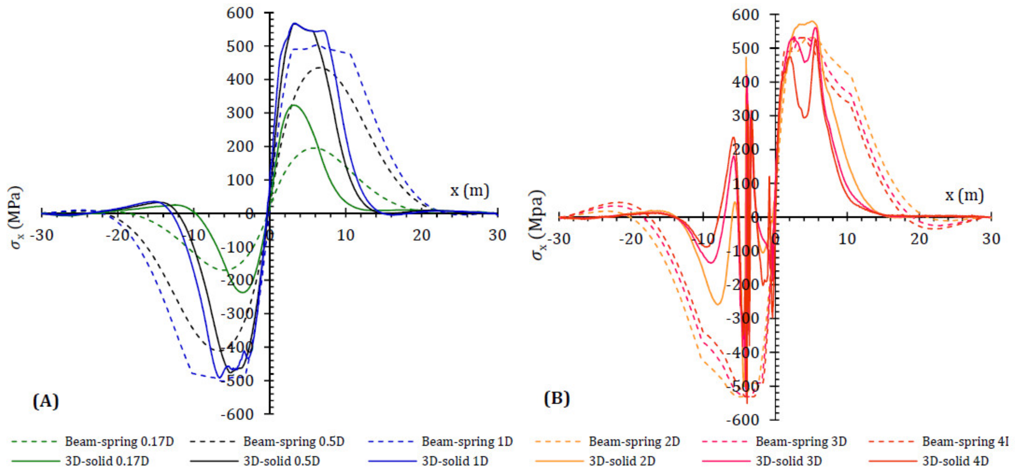
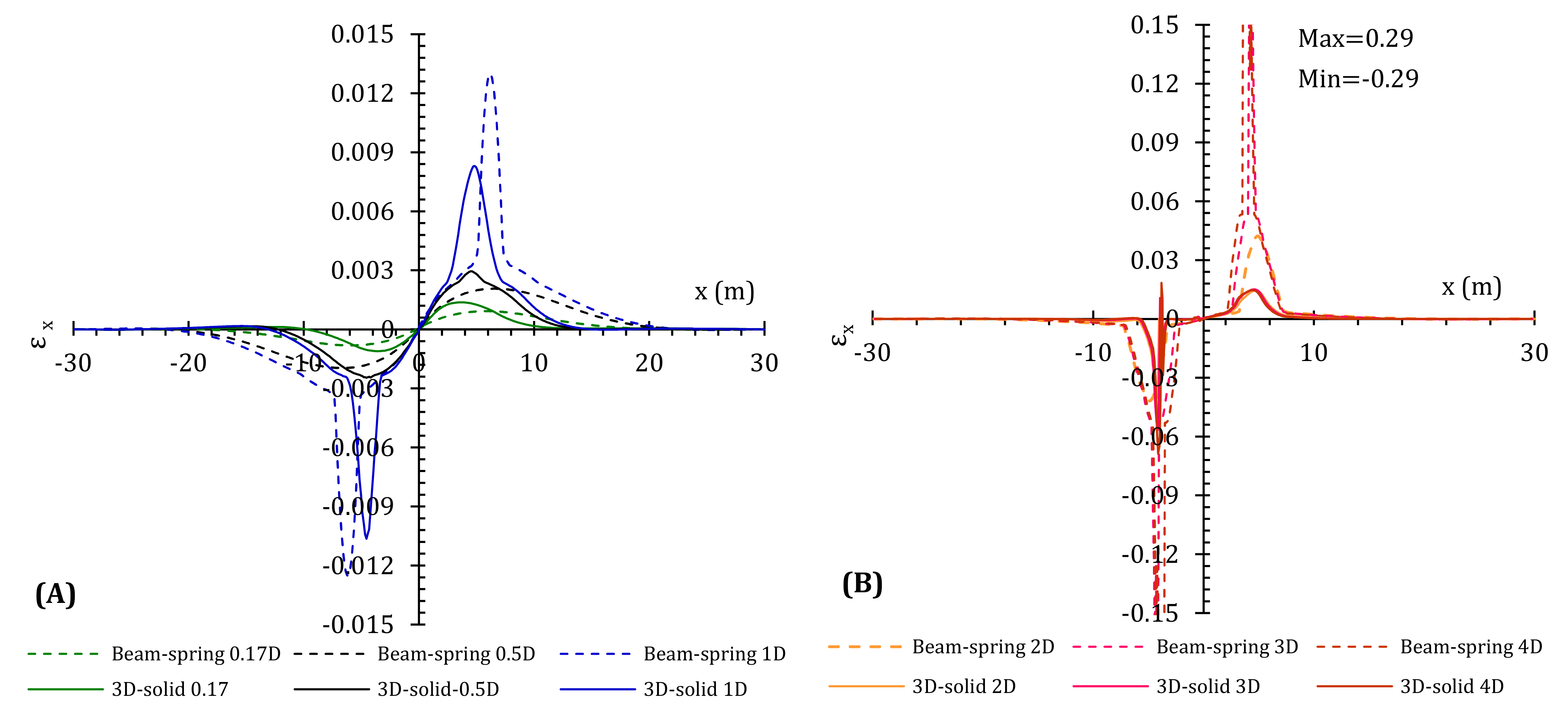
5.2. Analyses Results

The 3D solid and beam–spring FE models were analyzed with six cases with 60° strike-slip fault displacements of (δ) 0.17D, 0.5D, 1D, 2D, 3D, and 4D, where D is the pipe diameter.
Figure 14 shows the Mises stress outputs of the buried pipeline deformation modeled by the 3D solid method and its buckling for different fault movements. As seen, the pipeline starts buckling when the fault displacement is almost over 1D. Lateral displacements of the pipeline for both modeling approaches at the strike-slip fault crossing on a crown/invert of a pipe section (neutral axis) are compared in Figure 15.
In general, good compatibility is seen between the lateral displacement response of the buried pipeline for the 3D solid and beam–spring models.
However, due to a shorter high curvature zone of the 3D solid model than that of the beam–spring model, a gap can be seen around the faulting zone between the two model lateral displacement responses at the high curvature zone. Based on Equation (6), by increasing the soil stiffness and decreasing the pipe cross-section bending stiffness ( E I ), the high curvature zone length ( L c ) decreases. Since the material properties are identical in the 3D solid model and the beam–spring model, E is the same for both models. Therefore, a shorter high curvature zone length in the 3D solid models took place because of the local increasing soil stiffness at the faulting zone ( k ) and the decreasing of the inertia moment ( I ) of the pipe-section at the buckled locations. More precisely, the local stiffening of the soil in the 3D solid model is due to the local confinement of the soil at the fault line during the strike-slip fault movement. The beam–spring model cannot include the effects of soil confinement at the high curvature zone and local buckling of the buried pipe in the analysis, which are the main weakness of this modeling approach. Both modeling approaches present steady lateral displacement outside the high curvature zones. Furthermore, the lateral displacement results of the 3D solid model are lower than those of the beam–spring models at a steady-state range (further from the high curvature zone) for large fault movements (more than 2D). This happened because of the buckling of the buried pipeline at maximum bending moment locations (4–5 m from the fault plane) in the 3D solid model. Therefore, the strain energy release rate at the buckling location increased, and the strain rate in other locations along the pipeline decreased.
Stress and strain outputs are shown for the springline (point B in Figure 10) for the pipeline at both sides of the fault. The springline at the right side of the fault line has tensile stress, and the left side is in compression owing to the bending of the pipeline during faulting. As shown in Figure 16 and Figure 17, the distance between the maximum tensile/compression stress and the strain of the buried pipeline and fault line for the case of the 3D solid model is shorter than that of the beam–spring model. This is again because of the shortening of the high curvature zone due to the local stiffening of the soil and the local weakening of the I at the buckled zones in the 3D solid models.
Figure 16 and Figure 17 present the stress and strain outputs on the springline (point B in Figure 10) of the buried pipeline. Because of the symmetry of the problem, the results are shown only for one side of the pipe cross-section. The left springline of the pipe section has tensile stress and the right springline is in compression owing to the bending of the pipeline. As already discussed, local buckling in the pipeline occurs when the fault movement is almost over 1D. This local buckling affects the stress and strain responses. As shown in Figure 16 and Figure 17, the strain and stress responses of the buried pipeline before the appearance of local buckling in the 3D solid model ( δ 1 D ) were similar to the beam–spring model. However, the strain responses in the 3D solid model after buckling ( δ > 1 D ) were less than the beam–spring model. As shown in Figure 16 and Figure 17, the distance between maximum tensile/compression stress and strain of the buried pipeline and the faultline in the 3D solid models are shorter than the beam–spring model. This is again because of the shortening of the high curvature zone due to the local stiffening of the soil at the faulting zone and the local weakening of I at the buckled zones in the 3D solid models.
Because of the local stiffening of the soil around the high curvature zone and the local weakening of I at the buckled zones in the 3D solid models, the pipeline experienced higher stresses in the elastic range in comparison with the beam–spring model, and the maximum stress of the pipeline reached the yielding stress earlier than the beam–spring models. As shown in Figure 16, in the 3D solid model cases with ( δ > 1 D ), in locations where the longitudinal stress of the springlines on the pipe cross-sections have excided the yielding stress of the pipe material (490 MPa) at the local buckling hinges’ locations because of the dropping of the pipe’s bending stiffness, the stress response of the pipeline locally drops, and the stress oscillates because of wrinkles on the pipe. By increasing δ , the length of this local stress drop-zone increases. In a similar manner (Figure 17), in the 3D solid model cases, with the strain in cases with ( δ > 1 D ), the longitudinal strains of the pipeline in the local bending locations dropped and oscillated because of wrinkles along the pipe in those locations. Indeed, the pipeline strain on the springline in the beam–spring model drastically increased after the occurrence of local buckling in the 3D solid model, which represents that the pipeline was damaged. Therefore, large plastic strain in the beam–spring model is a criterion for damage detection in this modeling approach. Moreover, the pipeline experiences high stress at the elastic zone, and the pipeline yields in the 3D solid model earlier than in the beam–spring model owing to the local stiffening of the soil material around the high curvature zone.
Most of the buried pipeline designs are performed by beam–spring model analyses, and pipeline design guidelines are fitted for this modeling approach. However, none of the existing design guidelines have included the effect of local stiffening of the soil at the high curvature zone and the local weakening of the inertia moment of the pipe at buckled zones on buried pipelines’ force–displacement and stress-strain behavior. Local stiffening of the soil in high curvature zones of the pipe and local weakening of the inertia moment of the pipe at buckled zones can increase the soil–pipe interaction forces and, correspondingly, increase stresses and damage vulnerability to the buried pipelines. In other words, it causes the underestimation of forces on the buried pipeline at earthquake faults crossing. Therefore, it is recommended to assign stiffer nonlinear soil–pipe interaction spring properties to the high curvature zone of the pipeline than the rest of the pipeline in the beam–spring modeling approach.

6. Conclusions

In this study, six cases of buried pipelines subjected to a 60° strike-slip fault have been evaluated through beam–spring and 3D solid modeling approaches. Finally, the following have been found:
  • In the 3D solid model, because of the pressure and shear forces caused by the fault movement on the soil and pipeline around the high curvature zone, local confinement takes place, and soil stiffness surrounding the pipeline increases locally around the high curvature zone.
  • Because of the locally stiffening of the soil and the local weakening of the inertia moment of the pipe at buckled zones in the 3D solid models, the high curvature zone length of the pipeline is shorter than in the beam–spring models.
  • Due to the locally stiffening of the soil and the local weakening of the pipe cross-section moment of inertia in the 3D solid models, the soil–pipe interaction forces increase. Therefore, the buried pipeline in the 3D solid models before the occurrence of local buckling experiences higher stress and strain in comparison with the beam–spring models.
  • In the 3D solid models, damage to the pipeline is visually detectable. Whereas, in the beam–spring models, observation of a local large strain on the pipeline is the best criterion for damage (e.g., buckling and ovalization) evaluation of the buried pipelines.
  • In the 3D solid model, because of the local softening of the bending stiffness of the pipe cross-section, the pipe stress decreases at the buckled zone, which decreases the lateral deflection of the pipeline at further distances from the high curvature zone.
  • Creating the 3D solid model is much more complex than the beam–spring model and it is easy to make mistakes in modeling for an amateur analyst. Moreover, modeling and analyzing take much time and cost. However, it can reproduce detailed and accurate results and cover all phenomena.
  • Beam–spring models cannot include the effects of soil confinement at the high curvature zone and the local buckling of the buried pipe in the analysis, which are the main weaknesses of this modeling approach.
  • Existing buried pipeline design guidelines have not included the effect of the local stiffening of the soil and the local softening of the pipe’s moment of inertia in the analysis recommendation. Therefore, to prevent the underestimation of the forces on the pipeline in the beam–spring modeling approach, it is recommended to assign stiffer nonlinear soil–pipe interaction spring properties to the high curvature length of the pipeline than the rest of the pipeline.

Author Contributions

Both authors have read and agreed to the published version of the manuscript. Both authors contributed equally to this paper.

Funding

This work was supported by a Grant-in-Aid for Scientific Research (A) (17H01287 principal investigator: Junji Kiyono, Kyoto University).

Conflicts of Interest

The authors declare no conflict of interest.

References

  1. O’Rourke, M.J.; Liu, X. Response of Buried Pipelines Subject to Earthquake Effects; Monograph Series; Multidisciplinary Center for Earthquake Engineering Research (MCEER), USA: Buffalo, NY, USA, 1999. [Google Scholar]
  2. Aghabeigi, P.; Farahmand-Tabar, S. Seismic vulnerability assessment and retrofitting of historic masonry building of Malek Timche in Tabriz Grand Bazaar. Eng. Struct. 2021, 240, 112418. [Google Scholar] [CrossRef]
  3. Ariman, T.; Muleski, G.E. A review of the response of buried pipelines under seismic excitations. Earthq. Eng. Struct. Dyn. 1981, 9, 133–151. [Google Scholar] [CrossRef]
  4. Liang, J.; Sun, S. Site effects on seismic behavior of pipelines: A review. ASME J. Press. Vessel Technol. 2000, 122, 469–475. [Google Scholar] [CrossRef]
  5. O’Rourke, T.D.; Lane, P.A. Liquefaction Hazards and Their Effects on Buried Pipelines; Technical Report NCEER-89-0007; National Center for Earthquake Engineering Research: Buffalo, NY, USA, 1989. [Google Scholar]
  6. O’Rourke, T.D.; Palmer, M.C. Earthquake performance of gas transmission pipelines. Earthq. Spectra 1996, 20, 493–527. [Google Scholar] [CrossRef]
  7. Earthquake Engineering Research Institute. Kocaeli, Turkey Earthquake of August 17; EERI Special Earthquake Report; EERI: Oakland, CA, Canada, 17 August 1999. [Google Scholar]
  8. Uzarski, J.; Arnold, C. Chi-Chi, Taiwan, Earthquake of September 21, 1999 Reconnaissance Report; Earthquake Spectra 17 (Suppl. A); MCEER: Buffalo, NY, USA, 21 September 2001. [Google Scholar]
  9. Jennings, P.C. Engineering Features of the San Fernando Earthquake February 9, 1971; California Institute of Technology Report, CaltechEERL, California, 71–02; Caltech: Pasadena, CA, USA, 1971. [Google Scholar]
  10. MaCaffrey, M.A.; O’Rourke, T.D. Buried pipeline response to reverse faulting during the 1971 San Fernando Earthquake. ASME PVP 1983, 77, 151–159. [Google Scholar]
  11. Desmond, T.P.; Power, M.S.; Taylor, C.L.; Lau, R.W. Behavior of Large-Diameter Pipeline at Fault Crossings; ASCE: New York, NY, USA, 1995; pp. 296–303. [Google Scholar]
  12. Nakata, T.; Hasuda, K. Active fault I 1995 Hyogoken Nanbu earthquake. Kagaku 1995, 65, 127–142. [Google Scholar]
  13. Takada, S.; Nakayama, M.; Ueno, J.; Tajima, C. Report on Taiwan Earthquake; RCUSS, Earthquake Laboratory of Kobe University: Kobe, Japan, 1999; pp. 2–9. [Google Scholar]
  14. Kazama, M.; Noda, T. Damage statistics (Summary of the 2011 off the Pacific Coast of Tohoku Earthquake damage). J. Soils Found. 2012, 52, 780–792. [Google Scholar] [CrossRef] [Green Version]
  15. Wham, B.P.; Dashti, S.; Franke, K.; Kayen, R.; Oettle, N.K. Water supply damage caused by the 2016 Kumamoto Earthquake. J. Lowl. Technol. Int. 2017, 19, 165–174. [Google Scholar]
  16. Miyajima, M.; Fallahi, A.; Ikemoto, T.; Samaei, M.; Karimzadeh, S.; Setiawan, H.; Talebi, F.; Karashi, J. Site Investigation of the Sarpole-Zahab Earthquake, Mw 7.3 in SW Iran of November 12, 2017. JSCE J. Disaster FactSheets 2018. [Google Scholar]
  17. Bagriacik, A.; Davidson, R.A.; Hughes, M.W.; Bradley, B.A.; Cubrinovskic, M. Comparison of statistical and machine learning approaches to modeling earthquake damage to water pipelines. Soil Dyn. Earthq. Eng. 2018, 112, 76–88. [Google Scholar] [CrossRef]
  18. Manolis, G.D.; Beskos, D.E. Underground and Lifeline Structures. In Computer Analysis and Design of Earthquake Resistant Structures: A Handbook; Beskos, D.E., Anagnostopoulos, S.A., Eds.; CMP: Southampton, UK, 1997; pp. 775–837. [Google Scholar]
  19. Nourzadeh, D.; Mortazavi, P.; Ghalandarzadeh, A.; Takada, S.; Ahmadi, M. Performance assessment of the Greater Tehran Area buried gas distribution pipeline network under liquefaction. Soil Dyn. Earthq. Eng. 2019, 124, 16–34. [Google Scholar] [CrossRef]
  20. O’Rourke, M.J.; Gadicherla, V.; Abdoun, T. Centrifuge modeling of PGD response of buried pipe. Earthq. Eng. Eng. Vib. 2005, 4, 69–73. [Google Scholar] [CrossRef]
  21. Palmer, M.C.; O’Rourke, T.D.; Stewart, H.E.; O’Rourke, M.J.; Symans, M. Large displacement soil-structure interaction test facility for lifelines. In Proceedings of the 8th US National Conference Commemorating the 1906 San Francisco Earthquake, EERI, San Francisco, CA, USA, 18–22 April 2006. [Google Scholar]
  22. O’Rourke, T.D.; Bonneau, A. Lifeline performance under extreme loading during earthquakes. In Earthquake Geotechnical Engineering; Pitilakis, K.D., Ed.; Springer: Dordrecht, The Netherlands, 2007; pp. 407–432. [Google Scholar]
  23. Lin, T.J.; Liu, G.Y.; Chung, L.L.; Chou, C.H.; Huang, C.W. Verification of Numerical Modeling in Buried Pipelines under Large Fault Movements by Small-Scale Experiments. In Proceedings of the 15WCEE, Lisbon, Portugal, 24–28 September 2012; Volume 9, pp. 6685–6693. [Google Scholar]
  24. Xie, X.; Symans, M.D.; O’Rourke, M.J.; Abdoun, T.H.; O’Rourke, T.D.; Palmer, M.C.; Stewart, H.E. Numerical 47odelling of buried HDPE pipelines subjected to strike-slip faulting. J. Earthq. Eng. 2011, 15, 1273–1296. [Google Scholar] [CrossRef]
  25. Ha, D.; Abdoun, T.H.; O’Rourke, M.J.; Symans, M.D.; O’Rourke, T.D.; Palmer, M.C.; Stewart, H.E. Buried high-density polyethylene pipelines subjected to normal and strike–slip faulting—A centrifuge investigation. Can. Geotech. J. 2008, 45, 1733–1742. [Google Scholar] [CrossRef]
  26. Ha, D.; Abdoun, T.H.; O’Rourke, M.J.; Symans, M.D.; O’Rourke, T.D.; Palmer, M.C.; Stewart, H.E. Centrifuge modelling of earthquake effects on buried high-density polyethylene (HDPE) pipelines crossing high curvature zones. ASCE J. Geotech. Geoenviron. Eng. 2008, 134, 1501–1515. [Google Scholar] [CrossRef]
  27. Abdoun, T.H.; Ha, D.; O’Rourke, M.J.; Symans, M.D.; O’Rourke, T.D.; Palmer, M.C.; Stewart, H.E. Factors influencing the behavior of buried pipelines subjected to earthquake faulting. Soil Dyn. Earthq. Eng. 2009, 29, 415–427. [Google Scholar] [CrossRef]
  28. Newmark, N.M.; Hall, W.J. Pipeline design to resist large fault displacement. In Proceedings of the U.S. National Conference on Earthquake Engineering, University of Michigan, Ann Arbor, MI, USA, 18–20 June 1975; pp. 416–425. [Google Scholar]
  29. Kennedy, R.P.; Chow, A.M.; Williamson, R.A. Fault movement effects on buried oil pipeline. ASCE Transp. Eng. J. 1977, 103, 617–633. [Google Scholar] [CrossRef]
  30. Kennedy, R.P.; Kincaid, R.H. Fault crossing design for buried gas oil pipelines. ASME PVP 1983, 77, 1–9. [Google Scholar]
  31. Wang, L.R.L.; Yeh, Y.A. A refined seismic analysis and design of buried pipeline for fault movement. Earthq. Eng. Struct. Dyn. 1985, 13, 75–96. [Google Scholar] [CrossRef]
  32. Karamitros, D.; Bouckovalas, G.; Kouretzis, G. Stress analysis of buried steel pipelines at strike-slip fault crossings. Soil Dyn. Earthq. Eng. 2007, 27, 200–211. [Google Scholar] [CrossRef]
  33. Trifonov, O.V.; Cherniy, V.P. A semi-analytical approach to a nonlinear stress–strain analysis of buried steel pipelines crossing active faults. Soil Dyn. Earthq. Eng. 2010, 30, 1298–1308. [Google Scholar] [CrossRef]
  34. Karamitros, D.K.; Bouckovalas, G.D.; Kouretzis, G.P.; Gkesouli, V. An analytical method for strength verification of buried steel pipelines at normal fault crossings. Soil Dyn. Earthq. Eng. 2011, 31, 1452–1464. [Google Scholar] [CrossRef]
  35. Trifonov, O.V.; Cherniy, V.P. Elastoplastic stress-strain analysis of buried steel pipelines subjected to fault displacements with account for service loads. Soil Dyn. Earthq. Eng. 2012, 33, 54–62. [Google Scholar] [CrossRef]
  36. Talebi, F.; Kiyono, J. Introduction of the axial force terms to governing equation for buried pipeline subjected to strike-slip fault movements. Soil Dyn. Earthq. Eng. 2020, 133, 106125. [Google Scholar] [CrossRef]
  37. Talebi, F.; Kiyono, J. A refined nonlinear analytical method for buried pipelines crossing strike-slip faults. Earthq. Eng. Struct. Dyn. 2021, 1–24. [Google Scholar] [CrossRef]
  38. Talebi, F.; Kiyono, J. Evaluation of modeling approaches for buried pipelines subjected to strike–slip fault movements. In Proceedings of the 17th World Conference of Earthquake Engineering (17WCEE), Sendai, Japan, 13–18 September 2020. [Google Scholar]
  39. Vazouras, P.; Dakoulas, P.; Karamanos, S.A. Pipe–soil interaction and pipeline performance under strike–slip fault movements. Soil Dyn. Earthq. Eng. 2015, 72, 48–65. [Google Scholar] [CrossRef]
  40. Liu, X.; Zhang, H.; Li, M.; Xia, M.; Zheng, W.; Wu, K.; Han, Y. Effects of steel properties on the local buckling response of high strength pipelines subjected to reverse faulting. J. Nat. Gas Sci. Eng. 2016, 33, 378–387. [Google Scholar] [CrossRef]
  41. Demirci, H.E.; Bhattacharya, S.; Karamitros, D.; Alexander, N. Experimental and numerical modelling of buried pipelines crossing reverse faults. Soil Dyn. Earthq. Eng. 2018, 114, 198–214. [Google Scholar] [CrossRef] [Green Version]
  42. Talebi, F.; Kiyono, J. Seismic response of buried pipelines to strong ground motion of strike-slip fault. In Landslides 5 Book, Understanding and Reducing Landslide Disaster Risk; Springer: Cham, Switzerland, 2020; pp. 55–60. Available online: https://link.springer.com/chapter/10.1007/978-3-030-60713-5_6.
  43. ABAQUS/CAE 2017. Dassault Systems Simulia Corp: Mayfield Heights, OH, USA, documentation of 2017 release.
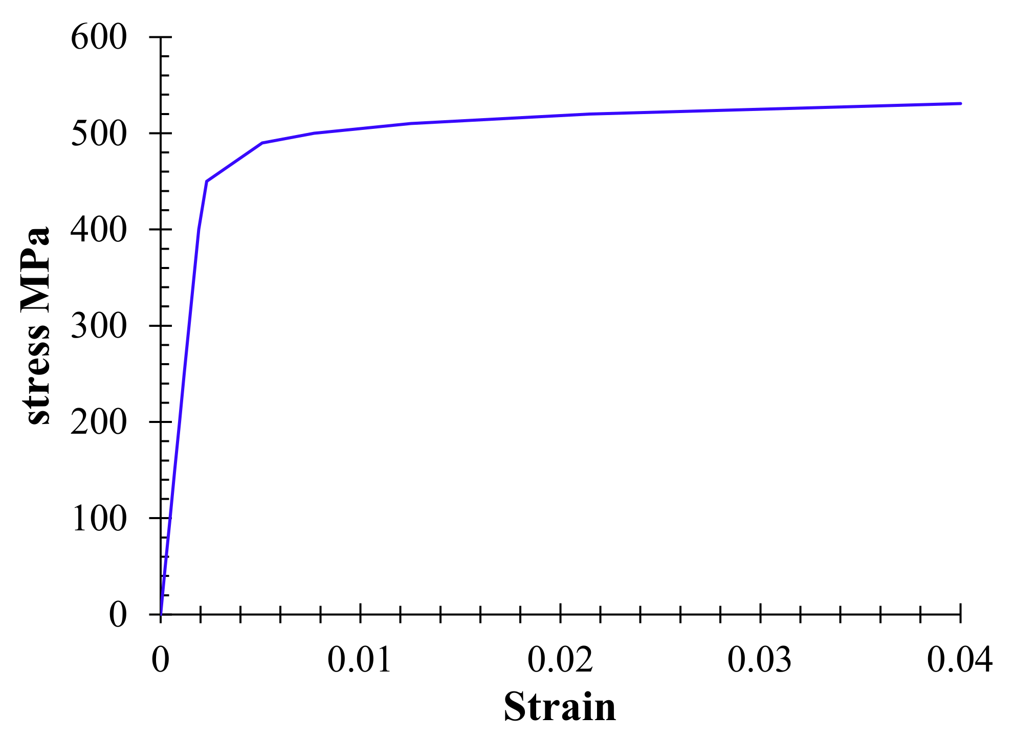
Figure 1. Buried pipeline subjected to a strike-slip fault with the faulting angle of (ψ).
Energies 14 04539 g001
Figure 2. High curvature length ( L c ) of the pipeline based on deflection w y .
Energies 14 04539 g002
Figure 3. 3D solid model for the pull-out test of the buried pipeline (displacement contours).
Energies 14 04539 g003
Figure 4. Shear stress–displacement relationship at the soil–pipe interface for friction coefficients of 0.2, 0.3, and 0.4. (a) This study, (b) Vazouras et al. [39].
Energies 14 04539 g004
Figure 5. Longitudinal soil–pipe force–displacement curves for contact friction coefficients of 0.2, 0.3, and 0.4 in pull-out tests by the 3D solid models.
Energies 14 04539 g005
Figure 6. Longitudinal soil–pipe force–displacement curve of the beam–spring model versus the 3D solid model in the pull-out test with a contact friction coefficient 0.3.
Energies 14 04539 g006
Figure 7. 3D solid model for the lateral sliding test of a buried pipeline (displacement contours).
Energies 14 04539 g007
Figure 8. Lateral soil–pipe force–displacement curves for contact friction coefficients of 0.2, 0.3, and 0.4 in lateral sliding tests by 3D solid models.
Energies 14 04539 g008
Figure 9. Lateral soil–pipe force–displacement curve of the beam–spring model versus the 3D solid model in a lateral sliding test with a contact friction coefficient of 0.3.
Energies 14 04539 g009
Figure 10. 3D solid model for a buried steel pipeline at a 60° strike-slip fault crossing. Points A and B are the springlines of the pipe.
Energies 14 04539 g010
Figure 11. Beam–spring model for a buried steel pipeline subjected at a 60° strike-slip fault crossing with a length of 60 m.
Energies 14 04539 g011
Figure 12. Equivalent nonlinear soil-pipe interaction springs in the beam–spring model. (a) Longitudinal, (b) Lateral, (c) Vertical.
Energies 14 04539 g012
Figure 13. Ramberg–Osgood stress–strain curve for steel API5L-X65.
Energies 14 04539 g013
Figure 14. The Mises stress response and buckled cross-section of a buried pipeline at a 60° strike-slip fault crossing in the 3D solid model for cases with fault movements of 0.17D, 0.5D, 1D, 2D, 3D, and 4D.
Energies 14 04539 g014
Figure 15. Lateral displacement of the buried pipeline subjected to a 60° strike-slip fault movement in the 3D solid model versus the beam–spring model on a crown/invert of a pipe cross-section, for cases with fault movements of 0.17D, 0.5D, 1D, 2D, 3D, and 4D.
Energies 14 04539 g015
Figure 16. Maximum/minimum longitudinal stresses of a buried pipeline subjected to a 60° strike-slip fault, 3D solid model versus beam–spring model. (A) Cases with a 0.17D to 1D fault movement; (B) cases with a 1D to 4D fault movement.
Energies 14 04539 g016
Figure 17. Maximum/minimum longitudinal strain of a buried pipeline subjected to a 60° strike-slip fault, 3D solid model versus beam–spring model. (A) Cases with a 0.17D to 1D fault movement; (B) cases with a 1D to 4D fault movement.
Energies 14 04539 g017
Table 1. Steel and soil properties.
ParameterX65 SteelSoil
Young’s Modulus (E)21 Tpa25 MPa
Poisson ratio (ν)0.30.5
Density (ρ)7850 kg/m32000 kg/m3
Cohesion (c)-50 kPa
Friction Angle (Φ)-
Yielding Stress ( σ y ) 490 MPa-
Yielding Strain ( ε y ) 0.233%-
Failure Stress ( σ f ) 531 MPa-
Failure Strain ( ε f ) 4%-
Table 2. Parameters of Ramberg–Osgood stress–strain for steel API5L-X65.
Initial Young’s modulus ( E )210 GPa
Yielding stress490 MPa
a38.31
r31.51
Publisher’s Note: MDPI stays neutral with regard to jurisdictional claims in published maps and institutional affiliations.

