Comparative Performance of Multi-Period ACOPF and Multi-Period DCOPF under High Integration of Wind Power

Abstract

Today, the power system operation represents a challenge given the security and reliability requirements. Mathematical models are used to represent and solve operational and planning issues related with electric systems. Specifically, the AC optimal power flow (ACOPF) and the DC optimal power flow (DCOPF) are tools used for operational and planning purposes. The DCOPF versions correspond to lineal versions of the ACOPF. This is due to the fact that the power flow solution is often hard to obtain with the ACOPF considering all constraints. However, the simplifications use only active power without considering reactive power, voltage values and losses on transmission lines, which are crucial factors for power system operation, potentially leading to inaccurate results. This paper develops a detailed formulation for both DCOPF and ACOPF with multiple generation sources to provide a 24-h dispatching in order to compare the differences between the solutions with different scenarios under high penetration of wind power. The results indicate the DCOPF inaccuracies with respect to the complete solution provided by the ACOPF.

1. Introduction

Reducing greenhouse gas emissions is imperative for climate change mitigation, leading to increased investments in reducing conventional fossil fuel-based power generation [1,2,3]. Therefore, a massive effort has been made worldwide to integrate renewable energy technologies [4,5,6]. The increasing inclusion of renewable energy resources is revealing a number of challenges in the power system operation [7,8,9,10]. Additional challenges for power system operators, who must address their day-to-day responsibilities, such as transmission requirements, maintaining network reliability and maximizing social and economic welfare [11]. Managing electricity markets requires a day-to-day operational planning [12,13].

A fundamental tool in the operational planning is the Optimal Power Flow (OPF), an optimization problem commonly involved in market clearing and security assessment processes [14,15]. Mainly, OPF aims to minimize operational cost while both units and system constraints are satisfied [15]. Moreover, the OPF solution allows to obtain a complete solution for all electrical variables, such as voltage, angles, active power, reactive power among others [16].

Nonetheless, the power flow solution is often hard to obtain, especially for large systems, due to problems related to both numerical methods and the power flow problem itself [17,18]. Additionally, power system analysis requires appropriate models to carry out steady state operation and stability studies [19,20,21,22]. Therefore, there are a variety of approaches to find the solution for an OPF, among which the AC optimal power flow (ACOPF) and the DC optimal power flow (DCOPF) stand out.

Consequently, this paper proposes a detailed formulation of the DC and AC optimal power flow with multiple generation sources to provide a 24-h dispatching to meet demand requirements based on [23]. Particularly, this paper proposes a detailed analysis of power system operation using both ACOPF and DCOPF under different conditions to evaluate the changes in reactive power and its effect in the overall dispatching and costs. This paper presents a comparative analysis finding circumstances where the differences between the DCOPF and the ACOPF are notorious. This paper uses a classical formulation wherein the objective function of both models is used to minimize the overall cost of the system operation, taking into account power generation costs. The proposed formulation determines the optimal results for all generators, for each case, all of them under different operating conditions and scenarios in order to determine power systems conditions where there are differences between the ACOPF and the DCOPF solution.

This paper is structured in these sections: Section 2 presents the problem description and formulation. In Section 3, the power system case and their parameters are outlined. Then, using the described systems, both formulation are tested. The results are analyzed and discussed at the end of this section. Some concluding remarks on this topic are given in Section 4.

2. AC Optimal Power Flow and the DC Optimal Power Flow Comparison

The optimal power flow for the economical dispatch of power systems containing different types of generators, such as gas or coal-fired thermal and renewable sources generators, has been extensively studied [24,25,26,27]. Different formulations are used to find a solution, including AC optimal power flow (ACOPF) and DC optimal power flow (DCOPF).

The ACOPF problem has been studied extensively in the literature [28,29,30,31,32,33,34], and corresponds to a full characterization of the power flow equations considering active and reactive power. Because of the non-convexity of the power flow equations, solving ACOPF by global optimization is extremely complex [35]. This difficulty has been increased by the variability generated by the inclusion of renewable energies, and has led to different studies in this area [36,37,38,39,40].

On the other hand, the DCOPF uses some simplifications from the ACOPF in order to obtain a linear system, and thus, it is easier to solve, giving the viability of obtaining computer solutions [41,42]. Therefore, the DCOPF has been widely studied and used in the recent years [43,44,45,46]. It has even been analyzed considering elements, such as uncertainty in electricity demand and wind availability [47,48,49]. Nevertheless, the DCOPF approach cannot provide information about reactive power, resistance and losses and voltage. Furthermore, the restriction of the degrees of freedom available, makes the solution less optimal and less precise [50,51].

3. Mathematical Formulation

This section includes the mathematical formulation for the DC-OPF dispatch model and the AC-OPF dispatch model. Both models include thermal and wind power generation. The two formulations are based on an optimization problem, designed to determine the lowest overall system operating cost, and derived from the production of electricity to meet demand over a 24-h period.

3.1. Formulation DC System

Equation (1) shows the total cost of electricity generation for a 24-h period as the sum of the cost of producing energy with g thermal units during a t time interval, plus the costs associated with non-utilization of the maximum wind generation source available.

$$EC=\sum _{g,t}{b}_g·P_g+\sum _{i,t}(VWC·P_{i,t}^{wc})$$

(1)

The dispatch model constraints are determined by the optimal power flow equations. The DC optimal power flow equilibrium is defined by Equation (2). The amount of power flowing in each line is determined by Equation (3). The constraints on the maximum amount of power that can flow through each line are given by the Equation (4).

$$\sum _g{P}_{g,t}+P_{i,t}^w-L_{i,t}=\sum _j{P}_{ij,t}$$

(2)

$$P_{ij,t}=\frac{1}{X_{ij}}\left({\theta }_{i,t}-{\theta }_{j,t}\right)$$

(3)

$${-P}_{ij,t}^{max}\le P_{ij,t}\le P_{ij,t}^{max}$$

(4)

On the other hand, the restrictions for thermal generation units are defined in Equations (5)–(7), where Equation (5) corresponds to the operational range of thermal generators. Equations (6) and (7) specify the maximum limits of the ramp-up and ramp-down of thermal generators, i.e., the maximum value that can vary the power of a generator in a one-hour interval.

$$P_{g,t}^{min}\le P_{g,t}\le P_{g,t}^{max}$$

(5)

$$P_{g,t}-P_{g,t-1}\le R_g^{up}$$

(6)

$${P_{g,t-1}-P}_{g,t}\le R_g^{down}$$

(7)

The constraints for wind generation are defined in Equations (8) and (9), where Equation (8) corresponds to to the amount of available wind power not utilized. Equation (9) indicates the range of minimum and maximum power that a wind turbine can produce, taking into account the capacity variables and wind availability.

$$P_{i,t}^{wc}=w_t·A_i-P_{i,t}^w$$

(8)

$$0\le P_{i,t}^w\le w_t·A_i$$

(9)

3.2. Formulation AC System

Equation (10) and, for the DC case, Equation (1), indicate the total cost of electricity generation for a 24-h period, plus the costs associated with non-utilization of the maximum wind generation source available.

$$EC=\sum _{g,t}{b}_g·P_g+\sum _{i,t}(VWC·P_{i,t}^{wc})$$

(10)

The restrictions for the dispatching model are given by the power flow equations. This section uses the AC approach to include power flow calculations. The active power flow balance is given by Equation (11). The reactive power flow balance is described by Equation (12). The active and reactive power flowing on each line is specified by Equations (13) and (14), respectively. The power flow restrictions are represented by the boundaries in Equation (15).

$$\sum _g{P}_{g,t}+P_{i,t}^w-L_{i,t}=\sum _j{P}_{ij,t}$$

(11)

$$\sum _g{Q}_{g,t}-{Lq}_{i,t}=\sum _j{Q}_{ij,t}$$

(12)

$$P_{ij,t}=\frac{V_{i,t}^2}{Z_{ij}}cos\left({\theta }_{ij}\right)-\frac{V_{ij}{V}_{ji}}{Z_{ij}}cos\left({\varphi }_{i,t}-{\varphi }_{j,t}+{\theta }_{ij}\right)$$

(13)

$$Q_{ij,t}=\frac{V_{i,t}^2}{Z_{ij}}sin\left({\theta }_{ij}\right)-\frac{V_{ij}{V}_{ji}}{Z_{ij}}sin\left({\varphi }_{i,t}-{\varphi }_{j,t}+{\theta }_{ij}\right)-\frac{b_{ij}{V}_{i,t}^2}{2}$$

(14)

$${-S}_{ij,t}^{max}\le S_{ij,t}\le S_{ij,t}^{max}$$

(15)

Furthermore, the restrictions for thermal generation units are defined in Equations (16)–(19). Equation (19) indicates the operational range in reactive power of thermal generators.

$$P_{g,t}^{min}\le P_{g,t}\le P_{g,t}^{max}$$

(16)

$$P_{g,t}-P_{g,t-1}\le R_g^{up}$$

(17)

$${P_{g,t-1}-P}_{g,t}\le R_g^{down}$$

(18)

$$Q_{g,t}^{min}\le Q_{g,t}\le Q_{g,t}^{max}$$

(19)

Additionally, the restrictions for wind generation are defined in Equations (20) and (21), as for the DC case.

$$P_{i,t}^{wc}=w_t·A_i-P_{i,t}^w$$

(20)

$$0\le P_{i,t}^w\le w_t·A_i$$

(21)

4. Results and Discussion

In order to analyze the sensitivity of power flows to reactive power, a power system case is used to simulate operational conditions. In this section, different scenarios are evaluated, with a 24 h period to consider the dispatching of generators. All simulations were completed with a personal computer (PC) running Windows^® with an Intel^® Core I7+ 8300H processor @2.3 GHz with 12.00 GB RAM, using Ipopt^® Solver (3.12.10) under the JuMP 0.19.2 Julia platform [52].

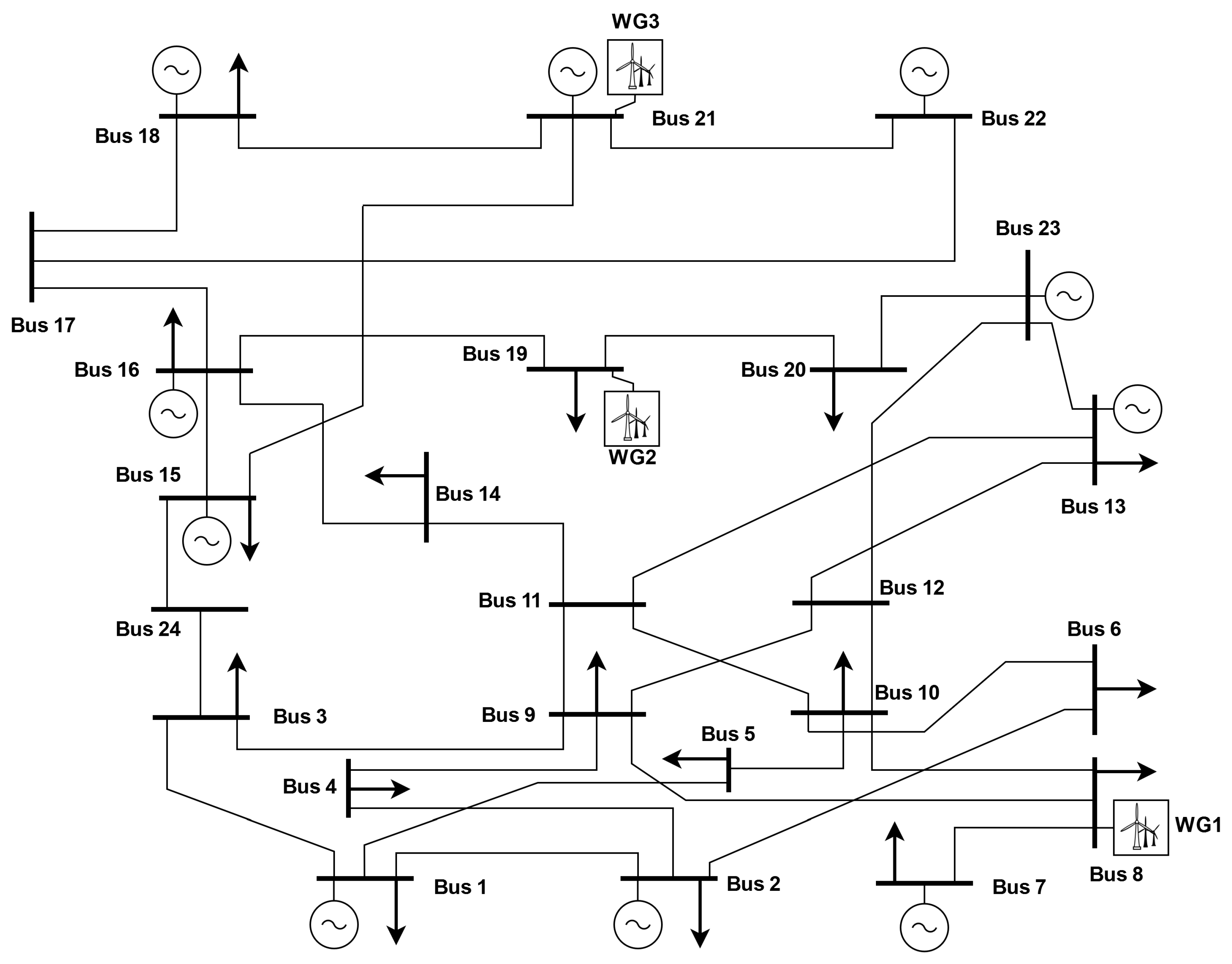
4.1. Case Description: IEEE 24-Bus

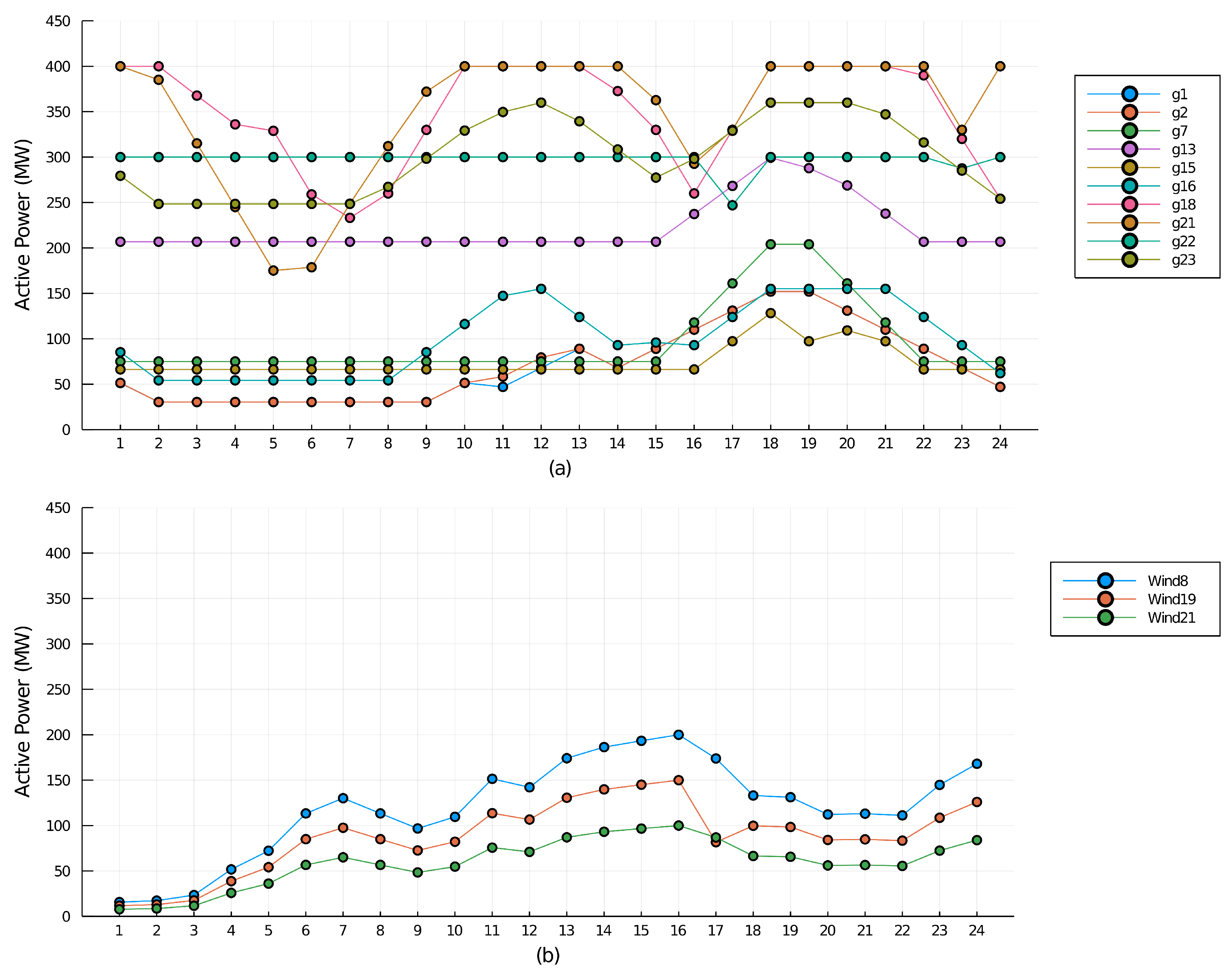
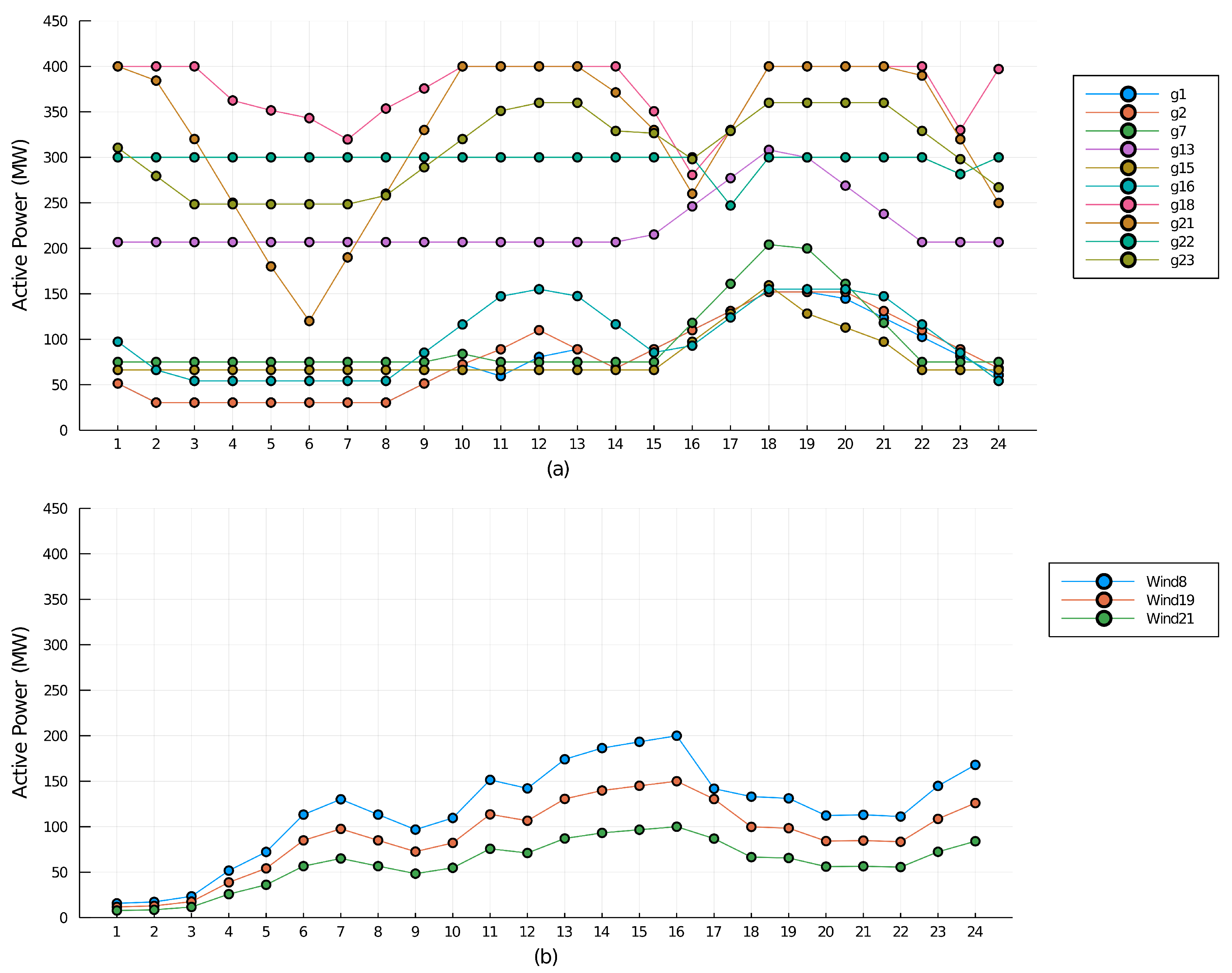
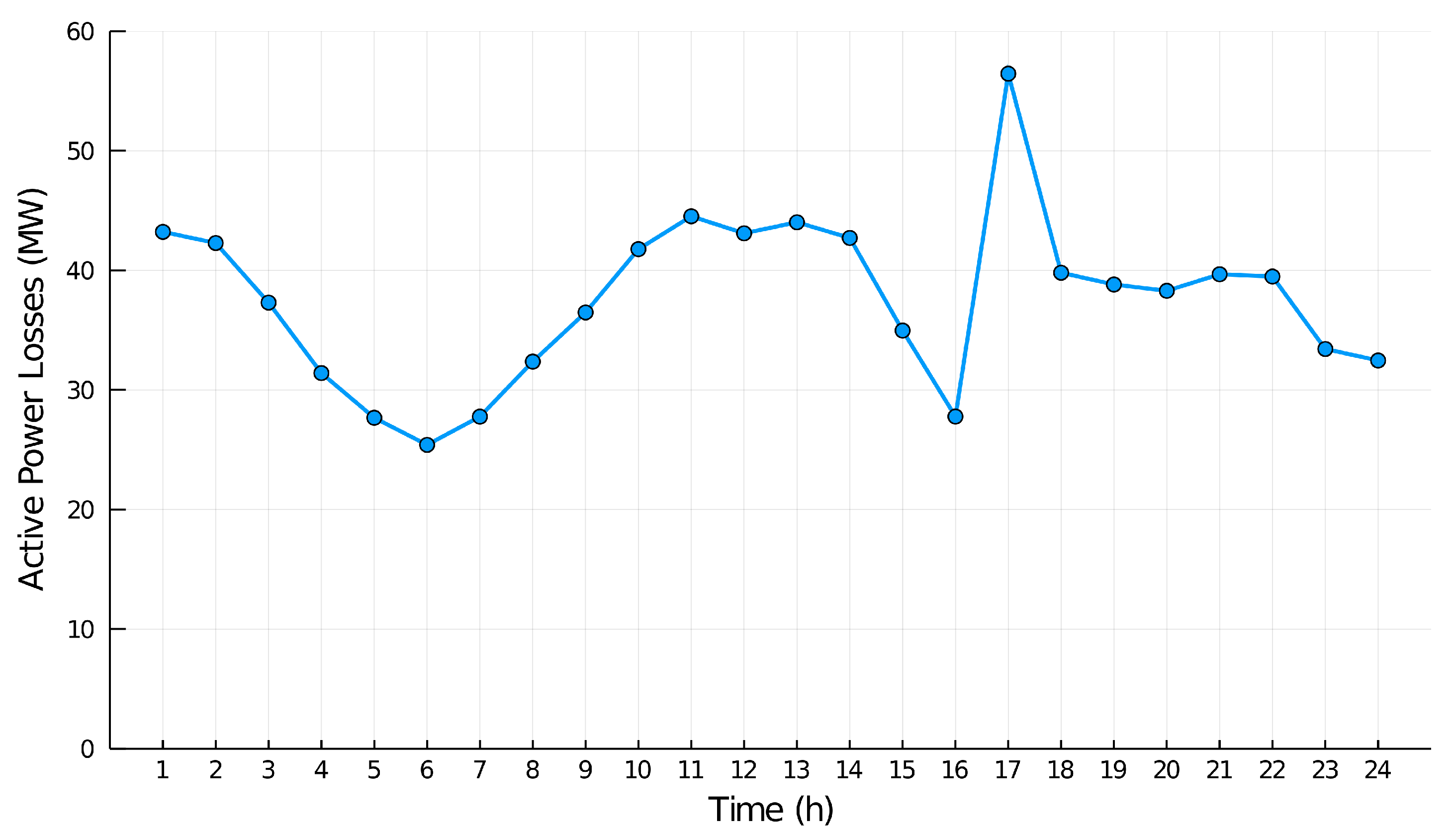
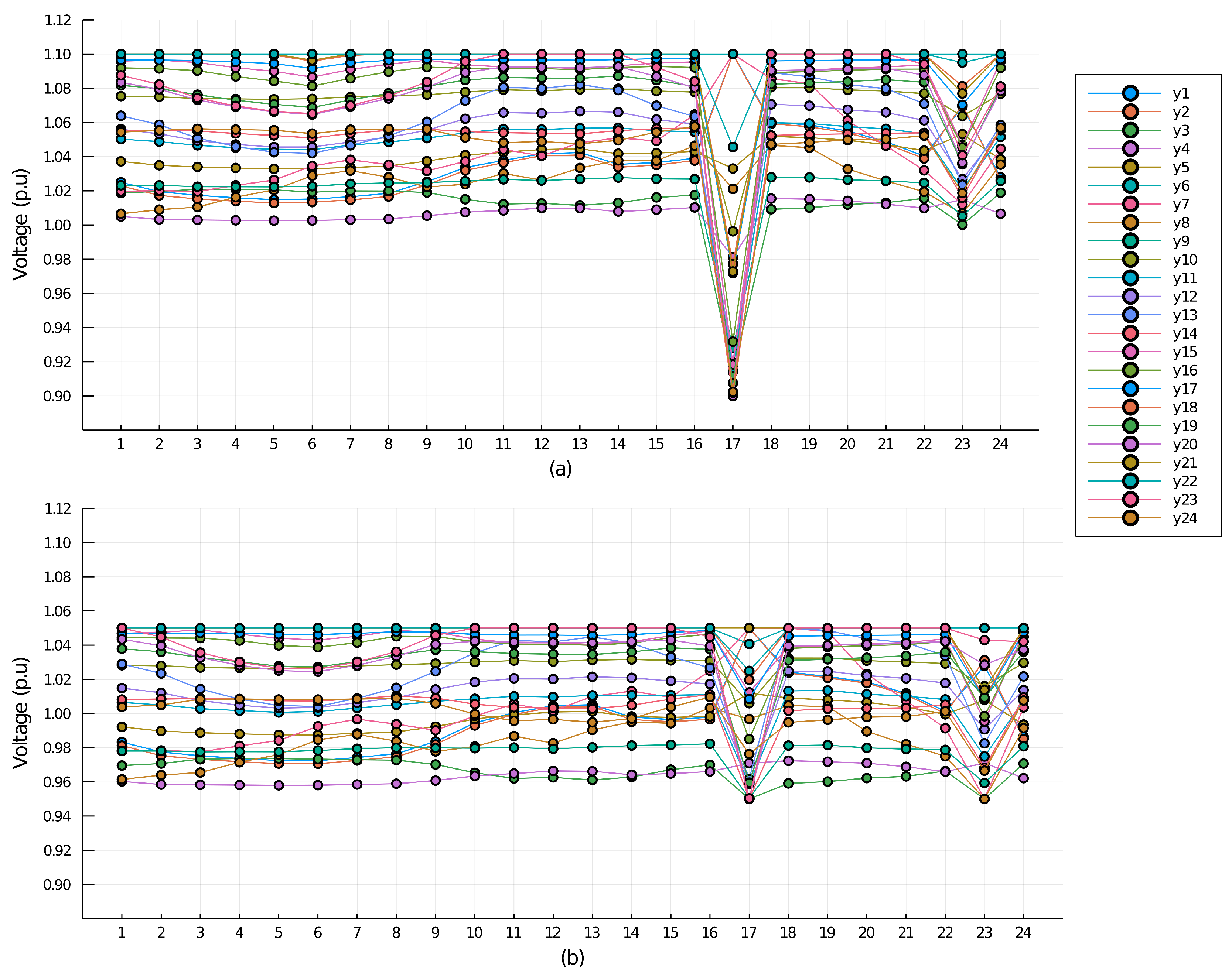
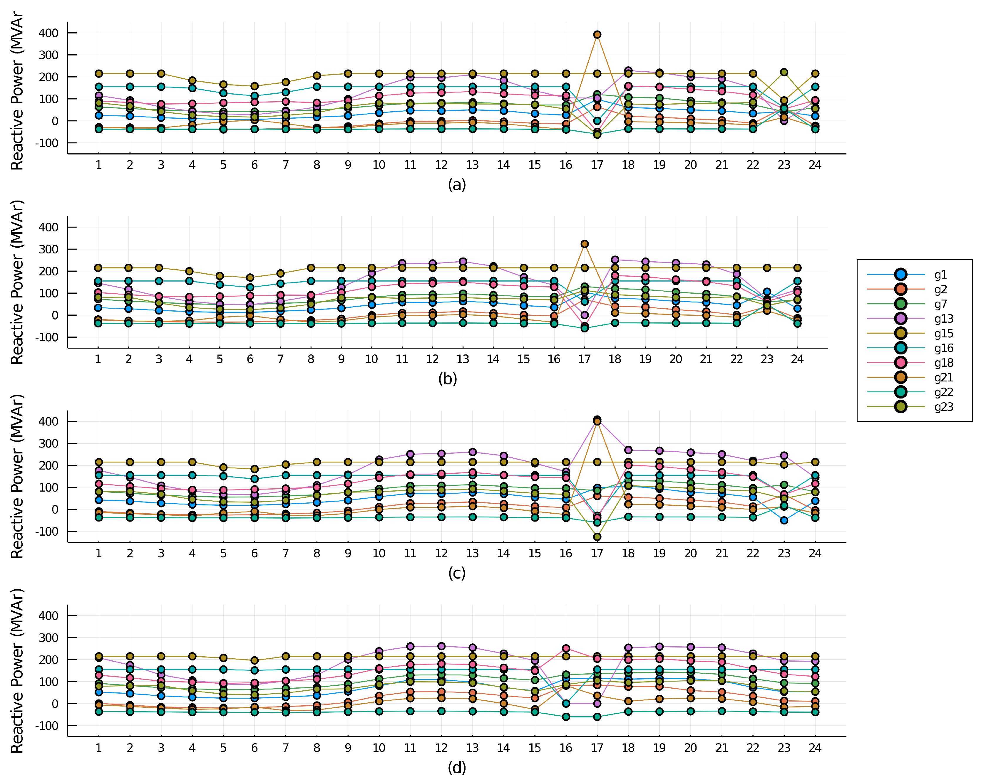
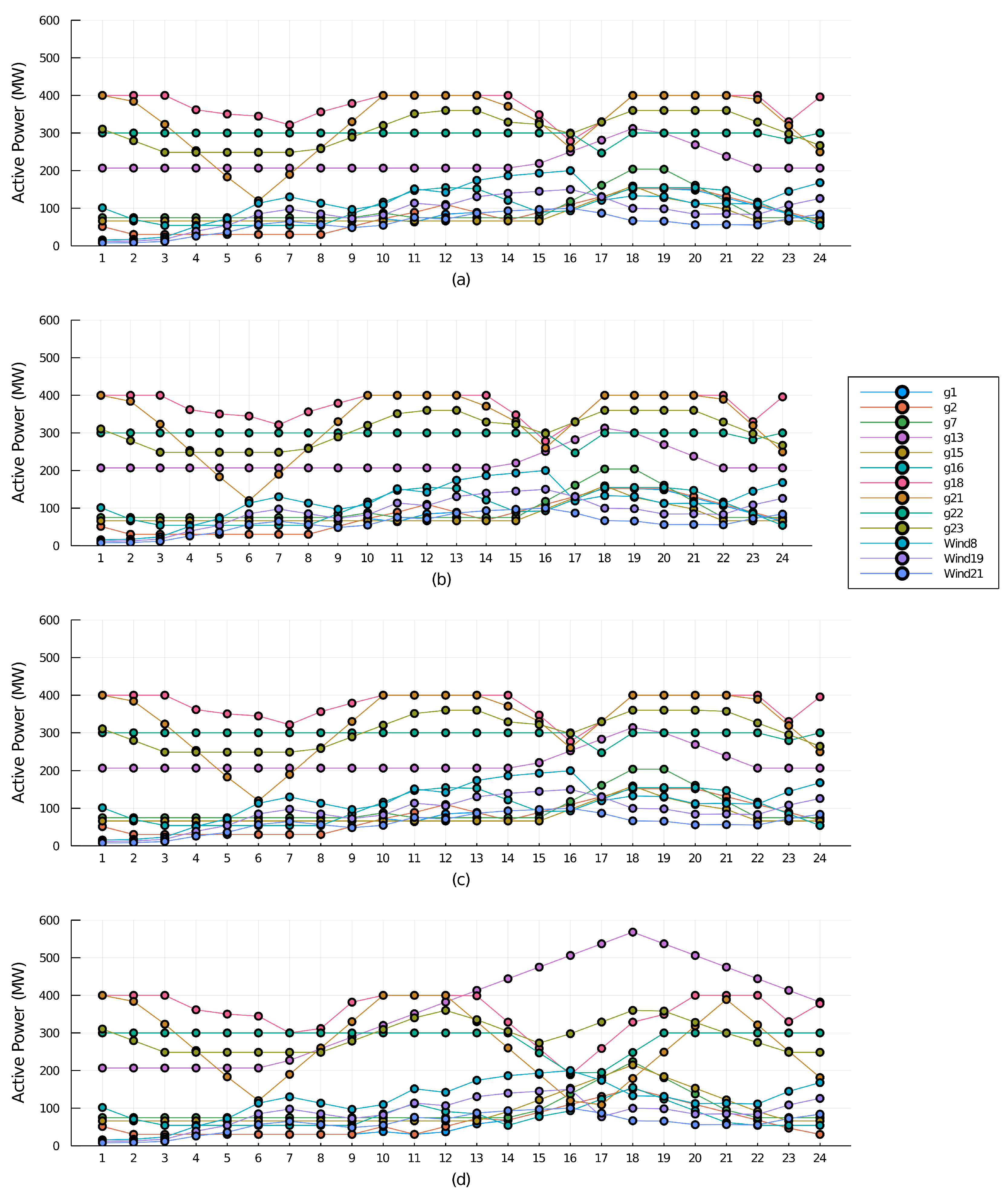
This section presents the results and simulations using the IEEE-24 bus system shown in Figure 1, considering different reactive power demand cases.

The IEEE 24-bus power system from [23] was slightly modified. The data for thermal units are shown in

Table 1. Thermal generation data for the 24-bus test system.

Gen	Bus	${\mathit{P}}_{\mathit{g}}^{\mathit{max}}$ (MW)	${\mathit{P}}_{\mathit{g}}^{\mathit{min}}$ (MW)	${\mathit{B}}_{\mathit{g}}$ ($/MW)	${\mathit{Q}}_{\mathit{g}}^{\mathit{max}}$ (MW)	${\mathit{Q}}_{\mathit{g}}^{\mathit{min}}$ (MW)	${\mathit{R}}_{\mathit{g}}$ (MW/h)
1	1	152	30.4	13.32	192	−50	21
2	2	152	30.4	13.31	192	−50	21
3	7	350	75	20.7	300	0	43
4	13	591	206.85	20.93	591	0	31
5	15	215	66.25	21	215	−100	31
6	16	155	54.25	10.52	155	−50	31
7	18	400	100	5.46	400	−50	70
8	21	400	100	5.47	400	−50	70
9	22	300	0	0	300	−60	53
10	23	360	248.5	10.52	310	−125	31

. This power system has three wind power plants, and the different sizes of these wind power plants are 250 MW, 150 MW and 100 MW connected to buses 8, 19 and 21, respectively. The system’s daily wind-demand variation patterns for all systems are plotted in Figure 2. In

Table 2. Branch data for the 24-bus test system.

From	To	${\mathit{r}}_{\mathit{ij}}$ (p.u)	${\mathit{X}}_{\mathit{ij}}$ (p.u)	${\mathit{b}}_{\mathit{ij}}$ (p.u)	Rating (MVA)
1	2	0.0026	0.0139	0.4611	175
1	3	0.0546	0.2112	0.0572	175
1	5	0.0026	0.0139	0.4611	175
2	4	0.0328	0.1267	0.0343	175
2	6	0.0497	0.192	0.052	175
3	9	0.0308	0.119	0.0322	175
3	24	0.0023	0.0839	0	250
4	9	0.0268	0.1037	0.0281	175
5	10	0.0228	0.0883	0.0239	175
6	10	0.0139	0.0605	2.459	250
7	8	0.0159	0.0614	0.0166	175
8	9	0.0427	0.1651	0.0447	175
8	10	0.0427	0.1651	0.0447	175
9	11	0.0023	0.0839	0	400
9	12	0.0023	0.0839	0	400
10	11	0.0023	0.0839	0	400
10	12	0.0023	0.0839	0	400
11	13	0.0061	0.0476	0.0999	500
11	14	0.0054	0.0418	0.0879	500
12	13	0.0061	0.0476	0.0999	500
12	23	0.0124	0.0966	0.203	500
13	23	0.0111	0.0865	0.1818	500
14	16	0.005	0.0389	0.0818	500
15	16	0.0022	0.0173	0.0364	500
15	21	0.0032	0.0245	0.206	1000
15	24	0.0067	0.0519	0.1091	500
16	17	0.0033	0.0259	0.0545	500
16	19	0.003	0.0231	0.0485	500
17	18	0.0018	0.0144	0.0303	500
17	22	0.0135	0.1053	0.2212	500
18	21	0.0017	0.013	0.109	1000
19	20	0.0026	0.0198	0.1666	1000
20	23	0.0014	0.0108	0.091	1000
21	22	0.0087	0.0678	0.1424	500

, the network grid information, such as the reactance, power line constraints and interconnections are shown, modified from [23].

4.2. Results

The results for this case are looking for differences in the dispatching using both ACOPF and DCOPF. Some scenarios are used to evaluate results of dispatching of active power, reactive power, costs, and voltage at different operating points. Additionally, some wind power values are used to determine the dispatching at different hours in order to identify critical points to be evaluated in detail. The simulations use the IEEE 24-Bus with the parameters indicated previously, to explore and evaluate the differences between the DCOPF and ACOPF model solutions, resulting from transmission line losses, voltage constraints and reactive power requirements.

Initially, the optimal power flow is realized using the DC case formulation, which is considered as the reference case. As a result, the optimal active power generation of thermal and wind power units over a 24-h period is obtained, and can be seen in Figure 3. According with the availability of wind power there are changes in the dispatching of some conventional generators, for instance, g18 and g21 at hours 4, 5, and 16. In addition, this optimal dispatch has a overall cost of $434,823.4.

Subsequently, an optimum power flow is determined using the AC case formulation, taking into account that the voltage of each bus had to remain at ±10% of its nominal magnitude (i.e., between 0.90 p.u. and 1.10 p.u.), and the angle between $-\pi$/2 and $\pi$/2. As a result, the optimal active power generation of thermal and wind power units over a 24-h period is obtained, and can be seen in Figure 4. This optimal dispatch has an overall cost of $447,921, which is 2.41% higher than the value of the DC case. This change is not only noticeable in the total cost, but also in the way thermal generators and wind turbine generators are dispatched in the 24-h period.

These variations depend on different factors, such as voltage restrictions, reactive power, and transmission line losses. For line losses, the factor in the case of DC, no line losses are considered; therefore, all the power generated by the thermal and wind units is for load supply only. In contrast, in the AC case, when considering the resistance, reactance and susceptance of the transmission lines, this leads to losses in the power flow among nodes. These losses depend on the power flow in the lines, and therefore, they vary every hour, as shown in Figure 5. For this case study, the 24-h losses were 901.2 MW, i.e., for the AC case, 901.2 MW more power had to be generated than in the DC case, which had to be supplied by the thermal units with high generation costs, resulting in an increase in the overall cost mentioned above.

Another factor to consider is voltage restrictions. This is due to the fact that in the case of DC, the magnitude of all bus voltages are 1.0 p.u, regardless of the optimal power flow dispatching solution. On the other hand, in the AC case, the voltage of the buses depends on the power flowing through them. Thus, the voltage in the buses varies over time; however, to obtain an optimal power flow, the magnitudes of the bus voltages should be maintained within a range close to 1.0 p.u. In order to analyze the effect of voltage restrictions, two cases were carried out, one where the voltage of each bus had to remain at ±10% of its nominal magnitude (i.e., between 0.90 p.u. and 1.10 p.u.), as shown in Figure 6a, and the second where the voltage of each bus had to remain at ±5% of its nominal magnitude (i.e., between 0.95 p.u. and 1.05 p.u.), as shown in Figure 6b.

For the case of voltage restriction at ±10%, it is found that the total cost of the system in the 24-h period was $447,921. On the other hand, for the voltage restriction case of 5, the overall system cost for the same period of time was $450,023, representing an increase of 0.47% compared to the previous case.

The increase in the overall cost is due to the fact that, as the voltage is restricted to values closer and closer to 1 p.u., the degrees of freedom of the model are reduced. Consequently, the solutions with a lower cost do not fulfill the constraints in certain hours, which results in variations in the optimal dispatch in accordance with the constraint. For example, it can be seen in Figure 6a that, for hour 17, the voltage at different nodes had an abrupt drop, but remained within the established parameters. However, for the case of Figure 6b, this drop cannot be so abrupt, which leads to a change in the dispatch of the thermal and wind generators compared to the previous case and thus is more costly.

Finally, the effect of reactive power on the optimal power flow solution was analyzed, using the ACOPF formulation. This case was performed, taking into account that the voltage of each bus had to remain at ±5% of its nominal magnitude (i.e., between 0.95 p.u. and 1.05 p.u.), and the angle between $-\pi$/2 and $\pi$/2.

The AC formulation performance was evaluated on the basis of an increase in reactive load, starting with the base case; thereafter, cases with a 10% increase of all the reactive load until reaching a 30% increase were considered. The analysis highlights the changes in power generation during a 24-h period of each generator, and therefore, the total cost of power generation for the same period of time.

Reactive power generation is performed by thermal generators, which must comply with the maximum and minimum reactor power generation restrictions shown in Table 2. In addition, the dispatch of reactives by the generators must comply with other restrictions, such as the magnitude and angle of voltage at the nodes, and the maximum apparent power that can flow through the lines. This means that as the reactive load increases, the dispatch changes in the 24-h period, as can be seen in Figure 7.

The base case of the ACOPF not only has a total cost different to the case of the DCOPF, but also the thermal units have the same active energy generation, as can be seen in Figure 7a. As of the 10% increase in the reactive load, changes in the OPF are beginning to be noticed, since for this case the total cost of energy generation was $437,407.2, which is 0.59% higher than the value of the DC case. This change is not only noticeable in the total cost, but also in the way thermal generators are dispatched in the 24-h period, as shown in Figure 7b.

For the $30\%$ increase in the reactive load, the changes are evident, because the total cost of power generation in this case was $461,026.3, which is 6.03% higher than the value of the DC case, meaning that for two versions of power systems with the same configuration and active load, the reactive load can increase the cost considerably. This change among cases is even more evident in the way thermal generators are dispatched in the 24-h period, and can be observed comparing the optimal active power generation of thermal units in DCOPF and ACOPF, shown in Figure 7c,d, respectively. For instance, the generator number 4, which is located on bus 13. For the DC case, at hour 18, it was dispatching a power of 300 MW, while in the same hour, for the AC case, it dispatched a power of 500 MW, corresponding to a variation of $66.6\%$. Meanwhile, Figure 8 shows the active power generation for each generator considering different levels of reactive power. As it can be seen, there are changes in active power at higher levels of reactive power, it means that in some circumstances the dispatch of active power changes, but the DCOPF model does not consider this changes because reactive power is neglected.

These results depend directly on the bus voltages. Considering that the voltage in a bus depends on the power flow and the load power factor, when the reactive load increases, some voltage magnitudes tend to decrease. Therefore, it is necessary that the power flow in these buses varies to comply with the voltage restriction. It is not recommended, in several occasions, to use the maximum capacity of wind power and use the most affordable generators at maximum capacity; instead, to use generators such that all restrictions are met, leading to an increase in total costs. Moreover, there are cases where an oversized increment in the reactive load causes that the optimal power flow model cannot comply with the voltage restriction; therefore, a solution is not found and the dispatch of the generators is not possible. As an illustration, there are cases of an increase of $40\%$ or more of the base reactive load, which do not converge because they do not meet all the restrictions. Furthermore, cost increases as reactive load grows may not be proportional, as shown in the results and illustrated in Figure 9.

5. Conclusions

In this document, two detailed models of economic dispatch for a 24-bus electric system that involves wind energy were presented under several operational settings for a 24-h time frame. It was demonstrated that the mathematical approach of both the ACOPF and DCOPF models presented corresponds to a valid approach to these elements for a planning process.

Power system operators are going to face increasing challenges in obtaining optimal power flows from a given system. For this reason, simplified models, such as the DCOPF, ought to be used, to facilitate obtaining an optimal solution, especially for cases with a high number of buses and generators. However, the simplified models are only an approximation and, in different cases, they must be verified.

Disregarding the reactive power in the optimal power flow can generate inaccurate results. This is because neither the generation and load nor the transmission of reactive power is considered. Besides, the magnitude of node voltages depends largely on the reactive power, and since these magnitudes must remain close to 1 p.u., the reactive flow becomes crucial.

In the evaluated scenarios, it could be observed that for cases of low reactive load, the differences between the economic dispatch solutions of the simplified DCOPF model and the ACOPF model were minimal. However, as the reactive load increased and the active load remained constant, the difference between the solutions of the two models became more significant.

References

1. Foley, A.; Olabi, A.G. Renewable energy technology developments, trends and policy implications that can underpin the drive for global climate change. Renew. Sustain. Energy Rev. 2017, 68, 1112–1114. [Google Scholar] [CrossRef] [Green Version]
2. Kasem, A.; Alawin, M. Exploring the Impact of Renewable Energy on Climate Change in The GCC Countries. Int. J. Energy Econ. Policy 2019, 9, 124–130. [Google Scholar] [CrossRef]
3. Hamels, S. CO2 Intensities and Primary Energy Factors in the Future European Electricity System. Energies 2021, 14, 2165. [Google Scholar] [CrossRef]
4. Ellabban, O.; Abu-Rub, H.; Blaabjerg, F. Renewable energy resources: Current status, future prospects and their enabling technology. Renew. Sustain. Energy Rev. 2014, 39, 748–764. [Google Scholar] [CrossRef]
5. Nasirov, S.; Cruz, E.; Agostini, C.A.; Silva, C. Policy Makers’ Perspectives on the Expansion of Renewable Energy Sources in Chile’s Electricity Auctions. Energies 2019, 12, 4149. [Google Scholar] [CrossRef]
6. Sanchez, F.; Gonzalez-Longatt, F.; Bogdanov, D. Probabilistic Assessment of Enhanced Frequency Response Services Using Real Frequency Time Series. In Proceedings of the 2018 20th International Symposium on Electrical Apparatus and Technologies (SIELA), Bourgas, Bulgaria, 3–6 June 2018; pp. 1–4. [Google Scholar] [CrossRef] [Green Version]
7. Carrasco, J.M.; Franquelo, L.G.; Bialasiewicz, J.T.; Galván, E.; PortilloGuisado, R.C.; Prats, M.M.; León, J.I.; Moreno-Alfonso, N. Power-electronic systems for the grid integration of renewable energy sources: A survey. IEEE Trans. Ind. Electron. 2006, 53, 1002–1016. [Google Scholar] [CrossRef]
8. Moreno, R.; Hoyos, C.; Cantillo, S. A Framework from Peer-to-Peer Electricity Trading Based on Communities Transactions. Int. J. Energy Econ. Policy (IJEEP) 2021, 11, 537–545. [Google Scholar] [CrossRef]
9. Moreno, R.; Larrahondo, D. The First Auction of Non-Conventional Renewable Energy in Colombia: Results and Perspectives. Int. J. Energy Econ. Policy (IJEEP) 2021, 11, 528–535. [Google Scholar] [CrossRef]
10. Shariatmadar, K.; Arrigo, A.; Vallée, F.; Hallez, H.; Vandevelde, L.; Moens, D. Day-Ahead Energy and Reserve Dispatch Problem under Non-Probabilistic Uncertainty. Energies 2021, 14, 1016. [Google Scholar] [CrossRef]
11. Lipka, P.; Oren, S.S.; O’Neill, R.P.; Castillo, A. Running a more complete market with the SLP-IV-ACOPF. IEEE Trans. Power Syst. 2016, 32, 1139–1148. [Google Scholar] [CrossRef]
12. Roald, L.; Andersson, G. Chance-constrained AC optimal power flow: Reformulations and efficient algorithms. IEEE Trans. Power Syst. 2017, 33, 2906–2918. [Google Scholar] [CrossRef] [Green Version]
13. Hinojosa, V.; Gonzalez-Longatt, F. Stochastic security-constrained generation expansion planning methodology based on a generalized line outage distribution factors. In Proceedings of the 2017 IEEE Manchester PowerTech, Manchester, UK, 18–22 June 2017; pp. 1–6. [Google Scholar] [CrossRef] [Green Version]
14. Capitanescu, F.; Ramos, J.M.; Panciatici, P.; Kirschen, D.; Marcolini, A.M.; Platbrood, L.; Wehenkel, L. State-of-the-art, challenges, and future trends in security constrained optimal power flow. Electr. Power Syst. Res. 2011, 81, 1731–1741. [Google Scholar] [CrossRef] [Green Version]
15. Kim, S.C.; Salkut, S.R. Optimal power flow based congestion management using enhanced genetic algorithms. Int. J. Electr. Comput. Eng. (2088-8708) 2019, 9. [Google Scholar] [CrossRef]
16. Frank, S.; Steponavice, I.; Rebennack, S. Optimal power flow: A bibliographic survey I. Energy Syst. 2012, 3, 221–258. [Google Scholar] [CrossRef]
17. Milano, F. Continuous Newton’s Method for Power Flow Analysis. IEEE Trans. Power Syst. 2009, 24, 50–57. [Google Scholar] [CrossRef]
18. Montoya, O.D.; Rueda, L.E.; Gil-González, W.; Molina-Cabrera, A.; Chamorro, H.R.; Soleimani, M. On the Power Flow Solution in AC Distribution Networks Using the Laurent’s Series Expansion. In Proceedings of the 2021 IEEE Texas Power and Energy Conference (TPEC), College Station, TX, USA, 2–5 February 2021; pp. 1–5. [Google Scholar] [CrossRef]
19. Moreno, R.; Florez, O. Online Dynamic Assessment of System Stability in Power Systems Using the Unscented Kalman Filter. Int. Rev. Electr. Eng. (IREE) 2019. [Google Scholar] [CrossRef]
20. Javadi, M.; Amraee, T. Mixed integer linear formulation for undervoltage load shedding to provide voltage stability. IET Gener. Transm. Distrib. 2018, 12, 2095–2104. [Google Scholar] [CrossRef]
21. Sridhar, J.; Prakash, R. Multi-objective whale optimization based minimization of loss, maximization of voltage stability considering cost of DG for optimal sizing and placement of DG. Int. J. Electr. Comput. Eng. (IJECE) 2019, 9, 835–839. [Google Scholar] [CrossRef]
22. Moreno, R. Identification of Topological Vulnerabilities for Power Systems Networks. In Proceedings of the 2018 IEEE Power & Energy Society General Meeting (PESGM), Portland, OR, USA, 5–9 August 2018. [Google Scholar] [CrossRef]
23. Soroudi, A. Power System Optimization Modeling in GAMS; Springer: Berlin/Heidelberg, Germany, 2017; pp. 148–150. [Google Scholar] [CrossRef]
24. Hakam, D.F. Nodal Pricing: The Theory and Evidence of Indonesia Power System. Int. J. Energy Econ. Policy 2018, 8, 135–147. [Google Scholar] [CrossRef]
25. Naveen, P.; Ing, W.K.; Danquah, M.K.; Abu-Siada, A.; Sidhu, A.S. Sustainable Economic and Emission Control Strategy for Deregulated Power Systems. Int. J. Energy Econ. Policy 2017, 7, 10. [Google Scholar]
26. Cantillo, S.; Moreno, R. Power system operation considering detailed modelling of energy storage systems. Int. J. Electr. Comput. Eng. (IJECE) 2021, 11, 182. [Google Scholar] [CrossRef]
27. Wang, Z.; Anderson, C.L. A Progressive Period Optimal Power Flow for Systems with High Penetration of Variable Renewable Energy Sources. Energies 2021, 14, 2815. [Google Scholar] [CrossRef]
28. Momoh, J.A. Electric Power System Applications of Optimization; CRC Press: Boca Raton, FL, USA, 2017. [Google Scholar]
29. Huneault, M.; Galiana, F. A survey of the optimal power flow literature. IEEE Trans. Power Syst. 1991, 6, 762–770. [Google Scholar] [CrossRef]
30. Zimmerman, R.D.; Murillo-Sánchez, C.E.; Thomas, R.J. MATPOWER: Steady-state operations, planning, and analysis tools for power systems research and education. IEEE Trans. Power Syst. 2010, 26, 12–19. [Google Scholar] [CrossRef] [Green Version]
31. Wang, H.; Murillo-Sanchez, C.E.; Zimmerman, R.D.; Thomas, R.J. On computational issues of market-based optimal power flow. IEEE Trans. Power Syst. 2007, 22, 1185–1193. [Google Scholar] [CrossRef]
32. Frank, S.; Rebennack, S. An introduction to optimal power flow: Theory, formulation, and examples. IIE Trans. 2016, 48, 1172–1197. [Google Scholar] [CrossRef]
33. Kang, S.; Kim, J.; Park, J.W.; Baek, S.M. Reactive power management based on voltage sensitivity analysis of distribution system with high penetration of renewable energies. Energies 2019, 12, 1493. [Google Scholar] [CrossRef] [Green Version]
34. Kanagaraj, A.; Raguru Pandu, K.D. Investigations of Various Market Models in a Deregulated Power Environment Using ACOPF. Energies 2020, 13, 2354. [Google Scholar] [CrossRef]
35. Lorca, A.; Sun, X.A. The adaptive robust multi-period alternating current optimal power flow problem. IEEE Trans. Power Syst. 2017, 33, 1993–2003. [Google Scholar] [CrossRef]
36. Dall’Anese, E.; Baker, K.; Summers, T. Chance-constrained AC optimal power flow for distribution systems with renewables. IEEE Trans. Power Syst. 2017, 32, 3427–3438. [Google Scholar] [CrossRef]
37. Ochoa, L.F.; Harrison, G.P. Minimizing energy losses: Optimal accommodation and smart operation of renewable distributed generation. IEEE Trans. Power Syst. 2010, 26, 198–205. [Google Scholar] [CrossRef] [Green Version]
38. Chamanbaz, M.; Dabbene, F.; Lagoa, C. AC optimal power flow in the presence of renewable sources and uncertain loads. arXiv 2017, arXiv:1702.02967. [Google Scholar]
39. Attarha, A.; Amjady, N.; Conejo, A.J. Adaptive robust AC optimal power flow considering load and wind power uncertainties. Int. J. Electr. Power Energy Syst. 2018, 96, 132–142. [Google Scholar] [CrossRef]
40. Bai, W.; Lee, D.; Lee, K.Y. Stochastic dynamic AC optimal power flow based on a multivariate short-term wind power scenario forecasting model. Energies 2017, 10, 2138. [Google Scholar] [CrossRef] [Green Version]
41. Cain, M.B.; O’neill, R.P.; Castillo, A. History of optimal power flow and formulations. Fed. Energy Regul. Comm. 2012, 1, 1–36. [Google Scholar]
42. Puangsukra, R.; Singh, J.G.; Ongsakul, W.; Gonzalez-Longatt, F.M. Multi-Objective Optimization for Enhancing System Coordination Restoration by Placement of Fault Current Limiters on an Active Distribution System with System Reliability Considerations. In Proceedings of the 2018 International Conference and Utility Exhibition on Green Energy for Sustainable Development (ICUE), Phuket, Thailand, 24–26 October 2018; pp. 1–9. [Google Scholar] [CrossRef]
43. Conejo, A.J.; Aguado, J.A. Multi-area coordinated decentralized DC optimal power flow. IEEE Trans. Power Syst. 1998, 13, 1272–1278. [Google Scholar] [CrossRef]
44. Montoya, O.D.; Grisales-Noreña, L.; González-Montoya, D.; Ramos-Paja, C.; Garces, A. Linear power flow formulation for low-voltage DC power grids. Electr. Power Syst. Res. 2018, 163, 375–381. [Google Scholar] [CrossRef]
45. Ou, M.; Xue, Y.; Zhang, X.P. Iterative DC optimal power flow considering transmission network loss. Electr. Power Components Syst. 2016, 44, 955–965. [Google Scholar] [CrossRef]
46. Hinojosa, V.H. Comparing Corrective and Preventive Security-Constrained DCOPF Problems Using Linear Shift-Factors. Energies 2020, 13, 516. [Google Scholar] [CrossRef] [Green Version]
47. Jabr, R.A. Adjustable Robust OPF With Renewable Energy Sources. IEEE Trans. Power Syst. 2013, 28, 4742–4751. [Google Scholar] [CrossRef]
48. Moreno, R.; Obando, J.; Gonzalez, G. An integrated OPF dispatching model with wind power and demand response for day-ahead markets. Int. J. Electr. Comput. Eng. (IJECE) 2019. [Google Scholar] [CrossRef]
49. Obando, J.S.; González, G.; Moreno, R. Quantification of operating reserves with high penetration of wind power considering extreme values. Int. J. Electr. Comput. Eng. (IJECE) 2020. [Google Scholar] [CrossRef]
50. Li, F.; Bo, R. DCOPF-based LMP simulation: Algorithm, comparison with ACOPF, and sensitivity. IEEE Trans. Power Syst. 2007, 22, 1475–1485. [Google Scholar] [CrossRef]
51. Soroush, M.; Fuller, J.D. Accuracies of optimal transmission switching heuristics based on DCOPF and ACOPF. IEEE Trans. Power Syst. 2013, 29, 924–932. [Google Scholar] [CrossRef]
52. Dunning, I.; Huchette, J.; Lubin, M. JuMP: A modeling language for mathematical optimization. SIAM Rev. 2017, 59, 295–320. [Google Scholar] [CrossRef]
Figure 1. IEEE 24-Bus.
Energies 14 04540 g001
Figure 2. Wind-demand variation patterns vs. time.
Energies 14 04540 g002
Figure 3. Active power generation of thermal units in Multi Period-DC OPF.
Energies 14 04540 g003
Figure 4. Active power generation of thermal units in Multi Period-AC OPF.
Energies 14 04540 g004
Figure 5. Active power losses in Multi-Period AC OPF.
Energies 14 04540 g005
Figure 6. Voltage power generation of thermal units in Multi Period-AC OPF.
Energies 14 04540 g006
Figure 7. Reactive power generation of thermal units in Multi Period-AC OPF.
Energies 14 04540 g007
Figure 8. Active power generation of thermal units in Multi Period-AC OPF.
Energies 14 04540 g008
Figure 9. Active power generation of thermal units in Multi Period-DC OPF.
Energies 14 04540 g009