Operating Cost Reduction in Distribution Networks Based on the Optimal Phase-Swapping including the Costs of the Working Groups and Energy Losses

Abstract

The problem of optimal phase-balancing in three-phase asymmetric distribution networks is addressed in this research from the point of view of combinatorial optimization using a master–slave optimization approach. The master stage employs an improved sine cosine algorithm (ISCA), which is entrusted with determining the load reconfiguration at each node. The slave stage evaluates the energy losses for each set of load connections provided by the master stage by implementing the triangular-based power flow method. The mathematical model that was solved using the ISCA is designed to minimize the annual operating costs of the three-phase network. These costs include the annual costs of the energy losses, considering daily active and reactive power curves, as well as the costs of the working groups tasked with the implementation of the phase-balancing plan at each node. The peak load scenario was evaluated for a 15-bus test system to demonstrate the effectiveness of the proposed ISCA in reducing the power loss (18.66%) compared with optimization methods such as genetic algorithm (18.64%), the classical sine cosine algorithm (18.42%), black-hole optimizer (18.38%), and vortex search algorithm (18.59%). The IEEE 37-bus system was employed to determine the annual total costs of the network before and after implementing the phase-balancing plan provided by the proposed ISCA. The annual operative costs were reduced by about 13% with respect to the benchmark case, with investments between USD 2100 and USD 2200 in phase-balancing activities developed by the working groups. In addition, the positive effects of implementing the phase-balancing plan were evidenced in the voltage performance of the IEEE 37-bus system by improving the voltage regulation with a maximum of 4% in the whole network from an initial regulation of $6.30\%$. All numerical validations were performed in the MATLAB programming environment.

1. Introduction

Three-phase distribution networks are responsible for interfacing transmission and sub-transmission networks at high-to-medium-voltage substations with end users at medium- and low-voltage levels [1,2]. These grids are typically built with a radial configuration to minimize the cost of investment in conductors and to simplify the process of protective device coordination [3]. The main challenge in three-phase distribution networks is to minimize the energy losses in the grid at minimal investment costs [4]. The energy losses in three-phase networks are mainly caused by the asymmetric nature of the matrix of impedances in all distribution lines, as well as the presence of multiple single-, two-, and three-phase loads [5]. Energy losses in electrical distribution networks can vary from 6 to 18% in the Colombian context [6]. These variations in the distribution networks depend on multiple factors, such as whether the connections are urban or rural, the length of the feeders, and the execution of maintenance plans. The Colombian regulatory environment for the electricity and gas sectors provides benefits via billing to distribution companies that demonstrate efficiency regarding energy loss indicators, thereby allowing them to transfer the costs of energy losses to all end users up to 8% [5]. This implies that if a distribution company has energy losses lower than this value, its distribution activities would generate an additional profit, whereas distribution companies with energy losses higher than 8% would not enjoy the advantage of this billing benefit. They would also incur additional operating costs that would reduce their net profit in the provision of the electricity service.

The extent of energy losses in three-phase networks can be lowered by employing different methodologies, such as shunt active and reactive power compensation [7,8], grid reconfiguration [9,10], and phase balancing [11,12]. The first two of these methodologies imply higher investment costs, as they require the acquisition of new equipment (i.e., capacitors, static compensators, and distributed generators), including the associated installation and maintenance costs [13]. On the other hand, the phase-balancing approach can be considered the most inexpensive method to reduce power losses because this method obviates the necessity for new devices [4], and the unique cost related to the phase-balancing plan is associated with working groups entrusted with traveling around to implement the required changes in the phases of the nodes of the grid [14]. In this study we solve the phase-balancing problem in an attempt to reduce the annual operating cost of three-phase distribution networks with asymmetric loads.

According to the latest literature, the problem of optimal phase balancing is typically studied with combinatorial optimization methods based on master–slave optimization strategies [15]. A few of these methodologies are described below. Cortés-Caicedo et al. [5] proposed the application of the vortex search algorithm (VSA) at the master stage combined with the classical backward/forward power flow in the slave stage. Their numerical results in test feeders composed of 8, 25, and 37 nodes demonstrated the efficiency of the VSA method when compared with classical genetic algorithms. In addition, all the results provided by the VSA were tested using DIgSILENT software, which confirmed the applicability of their methodology to real three-phase networks. Granada-Echeverri et al. [11] applied the classical Chu and Beasley genetic algorithm (CBGA) to solve the phase-balancing problem in two test feeders composed of 19 and 37 nodes. Their numerical results demonstrated the effectiveness of this optimization method in terms of the percentage of power loss reduction; however, they did not compare their approach with other metaheuristic approaches, which does not permit verification of the performance of the genetic algorithm in terms of processing times and solution repeatability. A simulated annealing method was proposed [4] for transformer swapping in three-phase asymmetric networks, and the approach was validated using a small test feeder composed of five nodes. The authors also compared their results with greedy and quenching algorithms to demonstrate the efficiency of the simulated annealing approach in reducing grid power losses. Authors of [16] proposed an improved version of the classical CBGA to solve the phase-balancing problem with an integer codification. The improvement consisted of the introduction on the selection, recombination, and mutation stages of a new operator based on the VSA to generate multiple offspring around a selected individual. This improvement helped the classical CBGA in the exploration and exploitation of the solution space in some promissory regions. Numerical results demonstrate the efficiency of the methodology when compared with the VSA, the classical CBGA, and the sine cosine algorithm, among others.

Additional methodologies applied to the phase-balancing problem include immune algorithms [12], artificial neural networks [17], fuzzy logic [18], a differential evolution algorithm [19], particle swarm optimization [20], and a bacterial foraging algorithm [21]. A different method to solve the phase-balancing problem was recently proposed in [22]. This involved the use of a mixed-integer quadratic approximation for redistributing the load connections among nodes in residential low-voltage microgrids. Although this approach ensures that the quadratic programming model finds the global optimum, the authors used a linear version of the three-phase power flow problem, which introduces estimation errors in the final solution. Authors of [23] presented a mixed-integer convex model to solve the load redistribution problem in three-phase asymmetric networks. The convex reformulation makes it possible find the global optimum of the approximated proposed model without considering the effect of the power balance equations in the optimization model; however, when the solution is evaluated in the exact phase-balancing formulation, the solutions provided by [23] correspond to locally optimal solutions. The authors of [24] proposed a linear programming formulation for the problem of phase balancing in three-phase networks. They did not consider the effect of the voltage magnitudes, since they were close to the substation voltage (i.e., 1.0 p.u.). Numerical results validated the proposed linear integer programming model in a small grid with six nodes; however, the authors did not provide comparisons with metaheuristics to confirm the effectiveness of their proposal.

Table 1. Main optimization methodologies applied to the phase-balancing problem in three-phase networks.

Optimization Method	Objective Function	Year	Reference
Simulated annealing algorithm	Power losses minimization	1999	[4]
Mixed-integer linear programming	Optimal current balancing	2006	[24]
Fuzzy logic approach	Power losses minimization	2007	[18]
Immune optimization algorithm	Power losses minimization	2008	[12]
Differential evolution algorithm	Power losses minimization	2012	[19]
Particle swarm optimization	Power losses minimization	2012	[20]
Bacterial foraging algorithm	Power losses minimization	2012	[21]
Chu and Beasley genetic algorithms	Power losses minimization	2012, 2020, 2021	[5,11,16]
Artificial neural networks	Power losses minimization	2014	[17]
Discrete vortex search algorithm	Power losses minimization	2020	[5]
Mixed-integer conic reformulation	Expected energy losses	2021	[22]
Mixed-integer convex approximation	Average unbalance level	2021	[23]

summarizes the main approaches reported in the literature to solve the problem of phase balancing in three-phase asymmetric distribution networks, which are based on metaheuristics and approximated convex models.

The main characteristic of the previous metaheuristic optimization methods listed in Table 1 is that they follow the leader–follower strategy. Here, the leader stage is entrusted by defining the load connections, and the follower stage solves the three-phase power flow problem to evaluate the objective function value, thereby helping guide the solution methodology through the solution space [25,26]. In addition, most of these studies only evaluated the phase-balancing methodology in the peak load condition and did not consider daily active and reactive power curves or the costs of the working groups that implement the final phase balancing along the test feeder.

The present research study makes the following contributions to the field:

• The use of an improved sine cosine algorithm (ISCA) to solve the phase-balancing problem; the algorithm was modified by changing the number of points in the codification that can change in each iterative cycle. This was achieved by using an adaptive rule as a function of the maximum number of nodes of the network.
• Hybridization of the ISCA (master stage) with the triangular-based three-phase power flow method (slave stage), which can solve power flow problems in asymmetric networks with loads with Y- and $\Delta$-connections.
• Evaluation of the phase-balancing plan by modifying the objective function to account for the annual costs of the energy losses (including daily active and reactive power curves) and the costs of the working groups that travel along the feeder to implement the optimization plan.

Importantly, the use of the ISCA to solve the phase-swapping problem in three-phase networks using master–slave optimization methodology has not previously been reported in the specialized literature. This is a gap in the current research that this work aims to fill. In addition, the results reported in this paper take into account the annual operating costs of the network by additionally considering the costs of deploying the working groups. This could be considered a reference point for the proposal of future optimization methodologies designed to address the problem of phase balancing in asymmetric three-phase networks.

The remainder of this document is structured as follows: Section 2 presents the general mixed-integer nonlinear programming model to represent the optimal phase-balancing problem in three-phase networks with a multi-period formulation; Section 3 describes the proposed optimization methodology based on the improved version of the sine cosine algorithm in the master stage and the triangular-based three-phase power flow method in the slave stage; Section 4 presents the main characteristics of the three-phase networks under study, which are composed of 15 and 37 nodes, respectively. Then, Section 5 presents the main numerical results obtained by the proposed ISCA in the 15- and IEEE 37-bus systems, considering the peak load scenario and daily active and reactive power curves. Furthermore, comparisons with four metaheuristic optimizers are provided to validate the effectiveness and robustness of our master–slave optimization proposal. Finally, Section 6 presents the concluding remarks derived from our research and outlines possible future work.

2. General Optimization Model

Electrical distribution networks are typically constructed with a three-phase structure such that they are as balanced as possible in terms of the impedances; however, the nature of the loads makes it impossible to ensure that the network is completely symmetrical, owing to the presence of single-, two-, and three-phase loads. This implies that the currents through all the lines are generally asymmetric [27,28], which significantly increases the energy losses of the network with respect to the ideal balanced case. Ultimately, this has a negative impact on the net profit of the distribution company in the electricity commercialization activity [29]. In order to address the problem of load balancing in three-phase networks, we propose an optimization model from the family of mixed-integer nonlinear programming (MINLP) methods, which are suitable for the analysis of multiperiod operating environments. The proposed optimization model attempts to minimize the annual operating cost of the network. These costs include the total costs of the energy losses summed with the costs of the phase-balancing task associated with the costs of displacing the crew working along the feeder. Note that the nonlinearities in the phase-balancing problem are related to the products of the trigonometric function and voltage magnitudes in the power balance constraints [30]. The integer part of the optimization model is related to the six possible load connections that are allowed at each node of the network [22]. The complete MINLP model is given in the following.

2.1. Objective Function

The structure of the objective function considered in this study corresponds to the summation of the costs incurred as a result of the annual energy loss and the cost of the phase balancing, which is associated with the displacement of the working group along the distribution feeder to implement the phase-balancing plan. Equation (1) defines the objective function used in this study.

$$A_{\cos \mathrm{t}}=f_1+f_2,$$

(1)

$$\begin{array}{c}{f}_1=C_{\mathrm{kWh}}T\sum _{t\in \mathcal{T}}\sum _{k\in \mathcal{N}}\sum _{m\in \mathcal{N}}\sum _{f\in \mathcal{F}}\sum _{g\in \mathcal{F}}{Y}_{kfmg}{V}_{kft}{V}_{mgt}cos\left({\delta }_{kft}-{\delta }_{mgt}-{\theta }_{kfmg}\right){\Delta }_t,\\ f_2=\sum _{k\in \mathcal{N}}{C}_{k,\mathrm{bal}}\underset{f\in \mathcal{F}}{max}\left\{\underset{g\in \mathcal{F}}{max}\left\{x_{kfg}-\left[\begin{array}{ccc}1& 0& 0\\ 0& 1& 0\\ 0& 0& 1\end{array}\right]\right\}\right\},\end{array}$$

where $A_{\mathrm{cost}}$ represents the total annual cost of the network operation, $f_1$ is the annual operating costs related with the total energy losses in all the branches of the network, and $f_2$ is the cost of the phase-balancing activity. $C_{\mathrm{kWh}}$ represents the average cost of the energy losses, T represents the number of hours in an ordinary year (i.e., 8760 h), $Y_{kfmg}$ represents the magnitude of the admittance that relates node k at phase f with node m at phase g, $V_{kft}$ ($V_{mft}$) corresponds to the voltage magnitude at node k (m) in phase f (g) at time period t, ${\delta }_{kft}$ (${\delta }_{mgt}$) is the angle of the voltage at node k (m) in phase f (g) at time period t, ${\theta }_{kfmg}$ represents the angle of the admittance that relates node k at phase f with node m at phase g, ${\Delta }_t$ is the time period during which the power demands remain constant, and $C_{k,\mathrm{bal}}$ is the cost of interchanging load phases at node k. Observe that $\mathcal{F}$, $\mathcal{N}$, and $\mathcal{T}$ are the sets that contain all the phases, nodes, and time periods, respectively.

2.2. Set of Constraints

The general set of constraints related to the phase-balancing problem in three-phase asymmetric networks includes active and reactive power balance equations, voltage regulation bounds, and conditions over the decision variables to maintain the feasibility of the solution space [5,22]. The set of constraints is as follows:

$$\begin{array}{c}\hfill P_{kft}^s-\sum _{g\in \mathcal{F}}{x}_{kfg}{P}_{kgt}^d=V_{kft}\sum _{m\in \mathcal{N}}\sum _{g\in \mathcal{F}}{Y}_{kfmg}{V}_{mgt}cos\left({\delta }_{kft}-{\delta }_{mgt}-{\theta }_{kfmg}\right),\left\{\begin{array}{c}\forall f\in \mathcal{F}\\ \forall k\in \mathcal{N}\\ \forall t\in \mathcal{T}\end{array}\right\},\end{array}$$

(2)

$$\begin{array}{c}\hfill Q_{kft}^s-\sum _{g\in \mathcal{F}}{x}_{kfg}{Q}_{kgt}^d=V_{kft}\sum _{m\in \mathcal{N}}\sum _{g\in \mathcal{F}}{Y}_{kfmg}{V}_{mgt}sin\left({\delta }_{kft}-{\delta }_{mgt}-{\theta }_{kfmg}\right),\left\{\begin{array}{c}\forall f\in \mathcal{F}\\ \forall k\in \mathcal{N}\\ \forall t\in \mathcal{T}\end{array}\right\},\end{array}$$

(3)

$$\begin{array}{c}\sum _{g\in \mathcal{F}}{x}_{kfg}=1,\left\{\forall f\in \mathcal{F},\forall k\in \mathcal{N},\forall t\in \mathcal{T}\right\},\end{array}$$

(4)

$$\begin{array}{c}\sum _{f\in \mathcal{F}}{x}_{kfg}=1,\left\{\forall g\in \mathcal{F},\forall k\in \mathcal{N},\forall t\in \mathcal{T}\right\},\end{array}$$

(5)

$$\begin{array}{c}{V}_{min}\le V_{kft}\le V_{max},\left\{\forall g\in \mathcal{F},\forall k\in \mathcal{N},\forall t\in \mathcal{T}\right\},\end{array}$$

(6)

where $P_{kft}^s$ and $Q_{kft}^s$ represent the active and reactive power generated by source s connected at node k in phase f in time period t, $P_{kgt}^d$ and $Q_{kgt}^d$ correspond to the active and reactive power demands connected at bus k in phase g at time period t, $x_{kfg}$ is a binary variable that determines the connection of the constant power consumption at bus k at f in phase g, and $V_{min}$ and $V_{max}$ are the minimum and maximum voltage regulation limits permitted for all buses of the electrical grid in each time period, respectively.

Remark 1.

The equality constraints (2) and (3), regarding the active and reactive power balance equations at each node, phase, and period of time, respectively, show the complexity of the three-phase unbalanced power flow problem in distribution grids, even when the connection of the loads at these nodes is perfectly known. Note that the main complication in these equations arises because of the need to calculate the products of the voltages and trigonometric functions, which necessitates the use of numerical methods to reach the solution within the desired convergence error [28].

2.3. General Model Interpretation

To understand the general formulation of the phase-balancing problem in asymmetric distribution networks, the following interpretations of Equations (1) and (6) are provided. Equation (1) is the objective function of the optimization problem. This function is intended to minimize the annual operating costs of the network, combining the costs of the energy losses with the cost of the phase-balancing implementation using working groups that travel along the feeder to implement the optimization plan. Equations (2) and (3) correspond to the active and reactive power balance equations for each node, phase, and time period in the three-phase distribution network, respectively. Note that in metaheuristic optimization methods with master–slave strategies these equations are solved numerically using methods such as the backward/forward power flow method [31], triangular-based power flow method [28], Newton–Raphson method, and graph-based approaches [32]. Equations (4) and (5) ensure that the loads are connected to the phases in a unique form by employing a matrix connection at each bus (i.e., node k), formed by the variables $x_{kfg}$, with the values in each column and each row of the matrix required to be equal to 1. Finally, the box-type Constraint (6) determines the upper and lower voltage regulation limits applicable to the electric distribution grid, which are typically $\pm 10\%$ for medium-voltage levels [5].

3. Solution Methodology

In this research, the problem of optimal phase balancing in three-phase networks is addressed from the point of view of master–slave optimization [15]. For the master stage, an improved sine cosine algorithm (ISCA) is proposed, whereas the slave stage is governed by solving the power flow problem for three-phase networks by using the recently developed triangular-based power flow method [28]. Note that the master stage is entrusted with determining the load configuration at each node of the network, whereas the slave stage is entrusted with the calculation of the costs incurred because of the energy loss during the period of analysis. In the following subsections, the master and slave stages are described in detail.

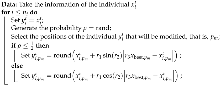
3.1. Master Stage: Improved Sine Cosine Algorithm

To determine the nodal connections of the three-phase loads, we propose an improved version of the sine cosine algorithm that explores and exploits the solution space by evolving through the solution space with trigonometric sine and cosine functions [33,34]. The main idea of the ISCA is to sweep the solution space using the information of the best current solution at iteration t (i.e., $x_{\mathrm{best}}$) and each individual $x_i^t$ in the population with weighted sine/cosine factors and a reduced number of modifications in the structure of the individual $x_i^t$, based on the adaptive rule.

The codification adopted to solve the phase-balancing problem is presented in

Table 2. Possible load connections in a three-phase node [5].

Connection Type	Phases	Sequence	Binary Variable ${\mathit{x}}_{\mathbf{kfg}}$
1	ABC		$\left[\begin{array}{ccc}1& 0& 0\\ 0& 1& 0\\ 0& 0& 1\end{array}\right]$
2	CAB	No change	$\left[\begin{array}{ccc}0& 0& 1\\ 1& 0& 0\\ 0& 1& 0\end{array}\right]$
3	BCA		$\left[\begin{array}{ccc}0& 1& 0\\ 0& 0& 1\\ 1& 0& 0\end{array}\right]$
4	ACB		$\left[\begin{array}{ccc}1& 0& 0\\ 0& 0& 1\\ 0& 1& 0\end{array}\right]$
5	BAC	Change	$\left[\begin{array}{ccc}0& 1& 0\\ 1& 0& 0\\ 0& 0& 1\end{array}\right]$
6	CBA		$\left[\begin{array}{ccc}0& 0& 1\\ 0& 1& 0\\ 1& 0& 0\end{array}\right]$

. Note that the binary variable $x_{kfg}$ can be easily represented with integer numbers between 1 and 6 [11].

The proposed classification for each individual $x_i^t$ in the ISCA is presented in Equation (7):

$$\begin{array}{c}\hfill x_i^t=\left[162\cdots 4\cdots 5\right],\end{array}$$

(7)

which produces an initial population with the form $I_p^t={\left[x_1^t{x}_2^t\cdots x_i^t\cdots x_{n_i}^t\right]}^T$ with $t=0$, where $n_i$ is the number of individuals in the population.

Remark 2.

Importantly, the codification presented in Equation (7) is feasible because each component of the individual $x_i^t$, i.e., $x_{ij}^t$, is generated with the following rule thereof:

$$\begin{array}{c}\hfill x_{ij}^t=round\left(x_{min}+\left(x_{min}-x_{max}\right)rand\right),\left\{\forall i=1,2,...,n_i,\forall j=1,2,...,n\right\},\end{array}$$

(8)

where $x_{min}=1$, $x_{max}=6$, $round\left(y\right)$ is a function that obtains the integer part of a real number, and rand is a random number between 0 and 1 generated with a normal distribution.

To generate the descending individuals, we propose a variation of the sine cosine algorithm that does not modify all the information of an individual in the same iteration. The general evolution of the ISCA is presented in Algorithm 1.

Algorithm 1: Generation of the descending individual.

In Algorithm 1, the parameter $\rho$ is determined for each individual if the evolution is made to occur using the sine or cosine function, $r_2$ is a random number between 0 and $2\pi$ generated with a normal distribution, and $r_3$ is a random number between 0 and 1 that determines the level of importance of the best current solution in the generation of the new individual. Note that $r_1$ is a variable factor that controls the balance between the exploration and exploitation of the solution space. This parameter is calculated as $r_1=1-\frac{t}{t_{max}}$, where $t_{max}$ is the maximum number of iterations specified for the ISCA.

Note that an important step prior to the evaluation of the descending individual $y_i^t$ is the verification of its upper and lower bounds, that is, $x_{min}\le y_{ij}^t\le x_{max}$. If either the upper or lower limit is violated, then the individual $y_{ij}^t$ is corrected by applying Equation (8).

To determine whether the descending individual $y_i^t$ will occupy the position $x_i^{t+1}$, the objective function value associated with the annual operating costs must be evaluated in the slave stage, which implies that if $A_{cost}\left(y_i^t\right)\le A_{cost}\left(x_i^t\right)$, then $x_i^{t+1}=y_i^t$.

The evolution process of the ISCA ends if one of the following criteria is met:

• If the maximum number of iterations $t_{max}$ is reached, then $x_{best}^{t_{max}}$ is reported as the optimal solution.
• If the objective function of the best solution does not improve during $k_{max}$ iterations, $x_{best}^{t_t}$ is reported as the optimal solution.

Remark 3.

The main advantage of using part of an individual to implement changes (i.e., the $p_m$ positions of the vector) is that the algorithm does not undertake large jumps through the solution space. This is necessary to control the exploration and exploitation properties of the algorithm, especially because of the discrete nature of the solution variables. The number of positions $p_m$ that will change varies between 1 and 10% of the number of variables of the problem, that is, n nodes.

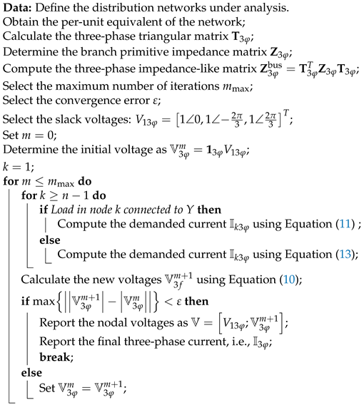
3.2. Slave Stage: Triangular-Based Power Flow Method

To evaluate each configuration provided by the master stage, we used the triangular-based three-phase power method that was recently proposed in [28]. The main advantages of this approach are its shorter processing times and its guarantee of convergence via the Banach fixed-point theorem [31]. The general formula for the triangular-based three-phase power flow method is presented below (taken from [28]):

$$\begin{array}{c}\hfill {\mathbb{V}}_{3\phi }={\mathbf{1}}_{3\phi }{V}_{13\phi }-{\mathbf{T}}_{3\phi }^T{\mathbf{Z}}_{3\phi }{\mathbf{T}}_{3\phi }{\mathbb{I}}_{3\phi },\end{array}$$

(9)

where ${\mathbb{V}}_{3\phi }\in {\mathcal{C}}^{3(n-1)\times 1}$ corresponds to a vector that contains all the phase voltages ordered per node, ${\mathbf{1}}_{3\phi }\in {\mathcal{R}}^{3(n-1)\times 3}$ corresponds to a rectangular matrix filled by $3\times 3$ identity matrices, $V_{13\phi }\in {\mathcal{C}}^{3\times 1}$ is a vector that contains the voltages of the substation node (voltage-controlled node), ${\mathbf{T}}_{3\phi }\in {\mathcal{R}}^{3b\times 3b}$ represents the three-phase equivalent of the upper-triangular matrix, ${\mathbf{Z}}_{3\phi }\in {\mathcal{C}}^{3b\times 3b}$ represents the primitive three-phase impedance matrix, which has a three-diagonal form, and ${\mathbb{I}}_{3\phi }\in {\mathcal{C}}^{3(n-1)\times 1}$ is a vector that contains all the phase currents ordered per node.

Note that Equation (9) must be solved iteratively because the voltages in all the demand nodes are indeed a function of the demanded currents (${\mathbb{I}}_{3\phi }$), which are functions of these voltages, that is, ${\mathbb{I}}_{3\phi }=f\left({\mathbb{V}}_{3\phi }\right)$. Equation (10) presents the recursive formula to solve the three-phase power-flow problem considering symmetric and asymmetric loads.

$$\begin{array}{c}\hfill {\mathbb{V}}_{3\phi }^{m+1}={\mathbf{1}}_{3\phi }{V}_{13\phi }-{\mathbf{T}}_{3\phi }^T{\mathbf{Z}}_{3\phi }{\mathbf{T}}_{3\phi }{\mathbb{I}}_{3\phi }^m,\end{array}$$

(10)

where m is the iterative counter. In addition, the convergence criterion adopted in this research corresponds to the maximum error between the voltage variables in two consecutive iterations, that is, $max\left\{\left|\right|{\mathbb{V}}_{3\phi }^{m+1}|-|{\mathbb{V}}_{3\phi }^m\left|\right|\right\}\le \epsilon$, where $\epsilon$ is the maximum tolerance and it is assigned as $1\times {10}^{-10}$, as recommended in [35].

It is important to emphasize that the triangular-based power flow method defined by the recursive Formula (10) has the ability to work with loads with $\Delta$- and Y-connections, which implies that the current ${\mathbb{I}}_{3\phi }^m$ must be calculated as a function of the type of load. If we consider that at node k there exists a load with a Y-connection, then the method for calculating the demand current is defined by Equation (11).

$$\begin{array}{c}\hfill {\mathbb{I}}_{ka}=\frac{{\mathbb{S}}_{ka}^{★}}{{\mathbb{V}}_{ka}^{★}},\\ \hfill {\mathbb{I}}_{kb}=\frac{{\mathbb{S}}_{kb}^{★}}{{\mathbb{V}}_{kb}^{★}},\\ \hfill {\mathbb{I}}_{kc}=\frac{{\mathbb{S}}_{kc}^{★}}{{\mathbb{V}}_{kc}^{★}},\end{array}$$

(11)

where ${\mathbb{I}}_{ka}$, ${\mathbb{I}}_{kb}$, and ${\mathbb{I}}_{kc}$ are the current demands in phases a, b, and c, respectively; ${\mathbb{V}}_{ka}$, ${\mathbb{V}}_{kb}$, and ${\mathbb{V}}_{kc}$ are the voltages per phase, considering that the neutral point of the load is solidly grounded; and ${\mathbb{S}}_{ka}$, ${\mathbb{S}}_{kb}$, and ${\mathbb{S}}_{kc}$ correspond to the loads connected between each phase and the neutral point. Observe that ${\mathbb{X}}^{★}$ presents the conjugate operator of the variable or parameter $\mathbb{X}$.

In the case of loads with a $\Delta$-connection at node k, the demanded current is calculated as defined in Equation (13).

$$\begin{array}{c}\hfill {\mathbb{I}}_{ka}={\left(\frac{{\mathbb{S}}_{kab}}{{\mathbb{V}}_{ka}-{\mathbb{V}}_{kb}}\right)}^{★}-{\left(\frac{{\mathbb{S}}_{kca}}{{\mathbb{V}}_{kc}-{\mathbb{V}}_{ka}}\right)}^{★},\\ \hfill {\mathbb{I}}_{kb}={\left(\frac{{\mathbb{S}}_{kbc}}{{\mathbb{V}}_{kb}-{\mathbb{V}}_{kc}}\right)}^{★}-{\left(\frac{{\mathbb{S}}_{kab}}{{\mathbb{V}}_{ka}-{\mathbb{V}}_{kb}}\right)}^{★},\\ \hfill {\mathbb{I}}_{kc}={\left(\frac{{\mathbb{S}}_{kca}}{{\mathbb{V}}_{kc}-{\mathbb{V}}_{ka}}\right)}^{★}-{\left(\frac{{\mathbb{S}}_{kbc}}{{\mathbb{V}}_{kb}-{\mathbb{V}}_{kc}}\right)}^{★},\end{array}$$

(12)

where ${\mathbb{S}}_{kab}$, ${\mathbb{S}}_{kbc}$, and ${\mathbb{S}}_{kca}$ are the apparent power consumption between the connections between phases a and b, b and c, and c and a, respectively.

To generalize the implementation of the triangular-based power flow method, Algorithm 2 presents the pseudo-code to solve the recursive Formula (10) for a general three-phase network with symmetric and asymmetric loads.

Algorithm 2: General pseudo-code for triangular-based three-phase power flow with loads with $\Delta$- and Y-connections.

Once the power flow problem is solved using the triangular-based power flow methodology presented in Algorithm 1, the evaluation of the annual energy losses of the network necessitates the calculation of the total power losses in each period of time. This is accomplished using the following expressions:

$$\begin{array}{c}\hfill {\mathbb{J}}_{3\phi }={\mathbf{T}}_{3\phi }{\mathbb{I}}_{3\phi },\end{array}$$

(13)

$$\begin{array}{c}\hfill {\mathbb{E}}_{3\phi }={\mathbf{Z}}_{3\phi }{\mathbb{J}}_{3\phi },\end{array}$$

(14)

where ${\mathbb{J}}_{3\phi }$ represents the vector that contains all the currents in the branches of the network, and ${\mathbb{E}}_{3\phi }$ represents the voltage drops. Note that if we combine these vectors, then the grid power losses are reached as defined in Equation (15).

$$\begin{array}{c}\hfill {\mathbb{S}}_{\mathrm{loss}}={\mathbb{E}}_{3\phi }^T{\mathbb{J}}_{3\phi },\end{array}$$

(15)

where ${\mathbb{S}}_{\mathrm{loss}}$ corresponds to the apparent power losses in the network.

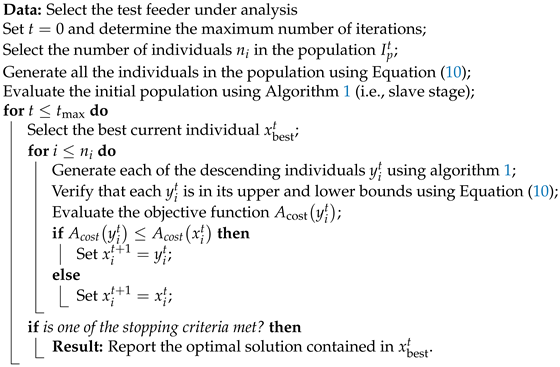
3.3. General Algorithm for the Proposed Master–Slave Optimizer

Algorithm 3 presents the pseudo-code with the optimization methodology designed to simplify the implementation of the proposed master–slave optimization approach. This method optimizes phase balancing in three-phase asymmetric networks with the ultimate aim of lowering the annual operating costs of the grid.

Algorithm 3: Master–slave optimization algorithm based on the ISCA and the triangular-based power flow method for phase balancing.

4. Test Feeders

The proposed master–slave optimization approach was validated using two test feeders in medium-voltage distribution networks composed of 15 and 37 nodes with radial topology, respectively. A description of each of these test feeders is presented below.

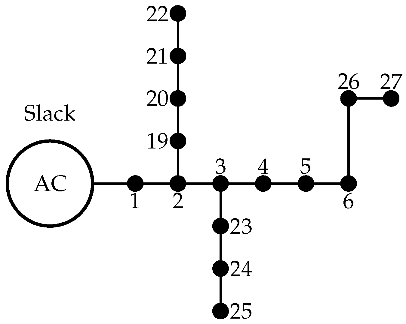
4.1. 15-Bus Test Feeder

This test feeder is composed of 15 nodes and 14 branches, with a voltage-controlled source connected at node 1, which is operated with a voltage magnitude of 13.2 kV. A single-phase diagram of this test feeder is presented in Figure 1. In addition, all the data for the 15-bus system are presented in

Table 3. Data of the 15-bus system (all power values are in kW and kvar).

Line	Node i	Node j	Cond.	Length (ft)	${\mathit{P}}_{\mathbf{ja}}$	${\mathit{Q}}_{\mathbf{ja}}$	${\mathit{P}}_{\mathbf{jb}}$	${\mathit{Q}}_{\mathbf{jb}}$	${\mathit{P}}_{\mathbf{jc}}$	${\mathit{Q}}_{\mathbf{jc}}$
1	1	2	1	603	0	0	725	300	1100	600
2	2	3	2	776	480	220	720	600	1040	558
3	3	4	3	825	2250	1610	0	0	0	0
4	4	5	3	1182	700	225	0	0	996	765
5	5	6	4	350	0	0	820	700	1220	1050
6	2	7	5	691	2500	1200	0	0	0	0
7	7	8	6	539	0	0	960	540	0	0
8	8	9	6	225	0	0	0	0	2035	1104
9	9	10	6	1050	1519	1250	1259	1200	0	0
10	3	11	3	837	0	0	259	126	1486	1235
11	11	12	4	414	0	0	0	0	1924	1857
12	12	13	5	925	1670	486	0	0	726	509
13	6	14	4	386	0	0	850	752	1450	1100
14	14	15	2	401	486	235	887	722	0	0

and

Table 4. Impedance parameters for the conductors in the 15-bus system.

Conductor		Impedance Matrix ($\mathbf{\Omega }/$mi)
	$0.3686+j0.6852$	$0.0169+j0.1515$	$0.0155+j0.1098$
1	$0.0169+j0.1515$	$0.3757+j0.6715$	$0.0188+j0.2072$
	$0.0155+j0.1098$	$0.0188+j0.2072$	$0.3723+j0.6782$
	$0.9775+j0.8717$	$0.0167+j0.1697$	$0.0152+j0.1264$
2	$0.0167+j0.1697$	$0.9844+j0.8654$	$0.0186+j0.2275$
	$0.0152+j0.1264$	$0.0186+j0.2275$	$0.9810+j0.8648$
	$1.9280+j1.4194$	$0.0161+j0.1183$	$0.0161+j0.1183$
3	$0.0161+j0.1183$	$1.9308+j1.4215$	$0.0161+j0.1183$
	$0.0161+j0.1183$	$0.0161+j0.1183$	$1.9337+j1.4236$

. Note that this information was adapted from [5].

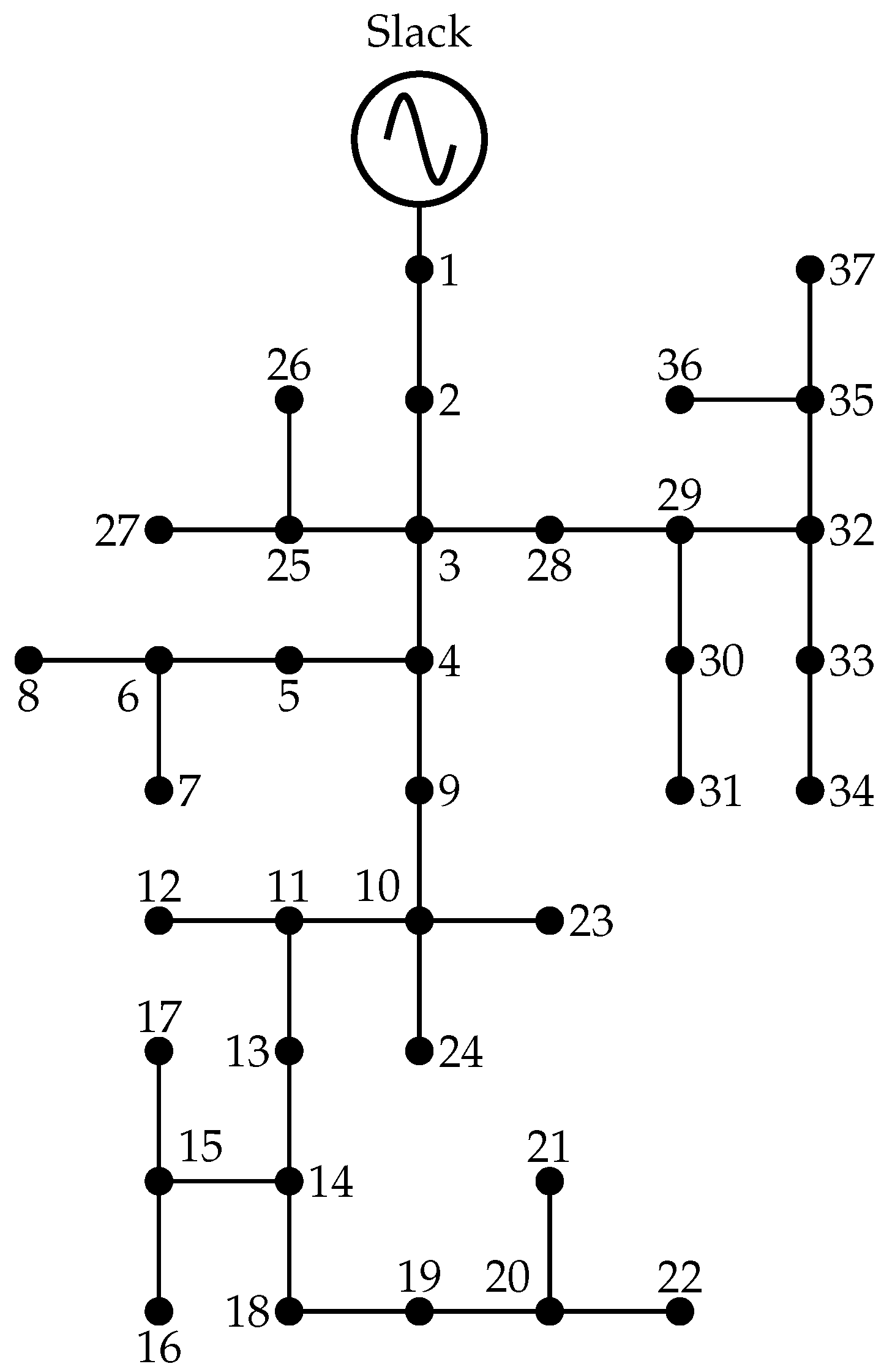
4.2. IEEE 37-Bus Test Feeder

This electrical network corresponds to a part of a real underground distribution system in California, USA. The network considered here is composed of 37 nodes and 36 lines with a radial configuration, where the slack source is located at node 1 and operated with a line-to-line voltage of 4.80 kV. The test system used in this study corresponds to the adaptation presented elsewhere [5]. The single-line diagram for this test feeder is presented in Figure 2, and the branches and loads as well as impedance information are presented in

Table 5. Data of the IEEE 37-bus system (all power values are in kW and kvar).

Line	Node i	Node j	Cond.	Length (ft)	${\mathit{P}}_{\mathit{ja}}$	${\mathit{Q}}_{\mathit{ja}}$	${\mathit{P}}_{\mathit{jb}}$	${\mathit{Q}}_{\mathit{jb}}$	${\mathit{P}}_{\mathit{jc}}$	${\mathit{Q}}_{\mathit{jc}}$
1	1	2	1	1850	140	70	140	70	350	175
2	2	3	2	960	0	0	0	0	0	0
3	3	24	4	400	0	0	0	0	0	0
4	3	27	3	360	0	0	0	0	85	40
5	3	4	2	1320	0	0	0	0	0	0
6	4	5	4	240	0	0	0	0	42	21
7	4	9	3	600	0	0	0	0	85	40
8	5	6	3	280	42	21	0	0	0	0
9	6	7	4	200	42	21	42	21	42	21
10	6	8	4	280	42	21	0	0	0	0
11	9	10	3	200	0	0	0	0	0	0
12	10	23	3	600	0	0	85	40	0	0
13	10	11	3	320	0	0	0	0	0	0
14	11	13	3	320	85	40	0	0	0	0
15	11	12	4	320	0	0	0	0	42	21
16	13	14	3	560	0	0	0	0	42	21
17	14	18	3	640	140	70	0	0	0	0
18	14	15	4	520	0	0	0	0	0	0
19	15	16	4	200	0	0	0	0	85	40
20	15	17	4	1280	0	0	42	21	0	0
21	18	19	3	400	126	62	0	0	0	0
22	19	20	3	400	0	0	0	0	0	0
23	20	22	3	400	0	0	0	0	42	21
24	20	21	4	200	0	0	0	0	85	40
25	24	26	4	320	8	4	85	40	0	0
26	24	25	4	240	0	0	0	0	85	40
27	27	28	3	520	0	0	0	0	0	0
28	28	29	4	80	17	8	21	10	0	0
29	28	31	3	800	0	0	0	0	85	40
30	29	30	4	520	85	40	0	0	0	0
31	31	34	4	920	0	0	0	0	0	0
32	31	32	3	600	0	0	0	0	0	0
33	32	33	4	280	0	0	42	21	0	0
34	34	36	4	760	0	0	42	21	0	0
35	34	35	4	120	0	0	140	70	21	10

and

Table 6. Impedance matrix for the type of conductors in the IEEE 37-bus test system.

Conductor		Impedance Matrix ($\mathbf{\Omega }/$mi)
	$0.2926+j0.1973$	$0.0673-j0.0368$	$0.0337-j0.0417$
1	$0.0673-j0.0368$	$0.2646+j0.1900$	$0.0673-j0.0368$
	$0.0337-j0.0417$	$0.0673-j0.0368$	$0.2926+j0.1973$
	$0.4751+j0.2973$	$0.1629-j0.0326$	$0.1234-j0.0607$
2	$0.1629-j0.0326$	$0.4488+j0.2678$	$0.1629-j0.0326$
	$0.1234-j0.0607$	$0.1629-j0.0326$	$0.4751+j0.2973$
	$1.2936+j0.6713$	$0.4871+j0.2111$	$0.4585+j0.1521$
3	$0.4871+j0.2111$	$1.3022+j0.6326$	$0.4871+j0.2111$
	$0.4585+j0.1521$	$0.4871+j0.2111$	$1.2936+j0.6713$
	$2.0952+j0.7758$	$0.5204+j0.2738$	$0.4926+j0.2123$
4	$0.5204+j0.2738$	$2.1068+j0.7398$	$0.5204+j0.2738$
	$0.4926+j0.2123$	$0.5204+j0.2738$	$2.0952+j0.7758$

, respectively.

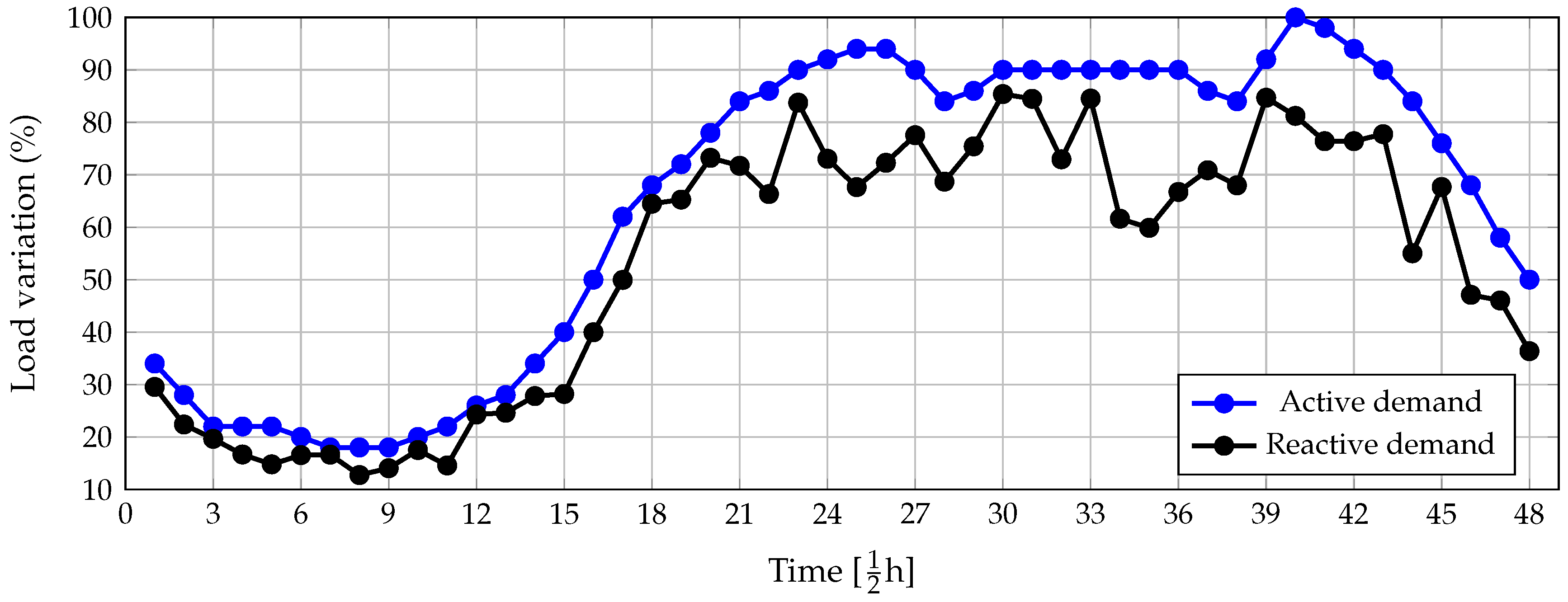
4.3. Behavior of the Demand in a Typical Working Day in Colombia

The effectiveness of the ISCA, in terms of performing the phase-balancing task for three-phase distribution networks, is demonstrated by considering the demand curves presented in Figure 3. The data used to plot these curves are also reported in

Table 7. Daily demand pattern in Colombia.

Period	Act. (pu)	React. (pu)	Period	Act. (pu)	React. (pu)
1	0.1700	0.1477	25	0.4700	0.3382
2	0.1400	0.1119	26	0.4700	0.3614
3	0.1100	0.0982	27	0.4500	0.3877
4	0.1100	0.0833	28	0.4200	0.3434
5	0.1100	0.0739	29	0.4300	0.3771
6	0.1000	0.0827	30	0.4500	0.4269
7	0.0900	0.0831	31	0.4500	0.4224
8	0.0900	0.0637	32	0.4500	0.3647
9	0.0900	0.0702	33	0.4500	0.4226
10	0.1000	0.0875	34	0.4500	0.3081
11	0.1100	0.0728	35	0.4500	0.2994
12	0.1300	0.1214	36	0.4500	0.3336
13	0.1400	0.1231	37	0.4300	0.3543
14	0.1700	0.1390	38	0.4200	0.3399
15	0.2000	0.1410	39	0.4600	0.4234
16	0.2500	0.1998	40	0.5000	0.4061
17	0.3100	0.2497	41	0.4900	0.3820
18	0.3400	0.3224	42	0.4700	0.3820
19	0.3600	0.3263	43	0.4500	0.3887
20	0.3900	0.3661	44	0.4200	0.2751
21	0.4200	0.3585	45	0.3800	0.3383
22	0.4300	0.3316	46	0.3400	0.2355
23	0.4500	0.4187	47	0.2900	0.2301
24	0.4600	0.3652	48	0.2500	0.1818

to enable our results to be compared with those in future research (note that the scaling factor of the data reported in Table 7 for active and reactive power demands is 2). Additional details regarding the active and reactive power daily behaviors presented in Table 7 can be consulted in [36].

Note that in the objective function we assume that the average energy cost is USD/kWh $0.1390$, which corresponds to the average cost of the energy in Bogotá, Colombia in May 2019 [36]. The number of days is considered to be 365 for an ordinary year, and the length of the power flow period, ${\Delta }_t$, is 0.5 h. In addition, the cost of the phase balancing of the working group is specified as USD 100 per node that requires intervention.

5. Numerical Analysis

In this section, we present the numerical results of the proposed master–slave optimization for solving the phase-balancing problem in three-phase asymmetric networks to minimize the annual grid operational costs. The following simulation scenarios are considered: (i) the evaluation of the numerical performance of the proposed ISCA on the 15-bus system considering the peak load condition, and (ii) the analysis of the annual operating cost of the network for the IEEE 37-bus system by employing the proposed ISCA.

5.1. Parametrization of the Optimization Algorithms

To determine the optimal population size for the proposed ISCA and the comparative optimization methodologies, we employed a grid generation with population sizes from 10 to 100 in steps of 5 in the 15-bus system for the peak load simulation case. The results were compared with those obtained using the following comparative methods: the classical Chu and Beasley genetic algorithm (CBGA) [11], classical sine cosine algorithm (SCA) [37], black-hole optimizer (BHO) [38], and vortex search algorithm (VSA) [5].

Table 8. General behavior of the proposed and comparative metaheuristics with different population sizes.

Method	Minimum (kW)	Maximum (kW)	Mean (kW)	Standard Deviation (kW)	Optimal Pop. Size
CBGA	109.2218	109.9080	109.5488	0.2075	75
BHO	109.5715	113.0922	110.7364	0.8377	95
SCA	109.5148	110.4816	109.9611	0.2492	85
VSA	109.2855	110.1828	109.6100	0.2485	80
ISCA	109.1980	109.6896	109.2952	0.1144	50

presents the general behavior of each of the optimization algorithms considering as performance indicators the minimum, maximum, mean and standard deviation.

The numerical results in Table 8 allow us to observe that:

✓

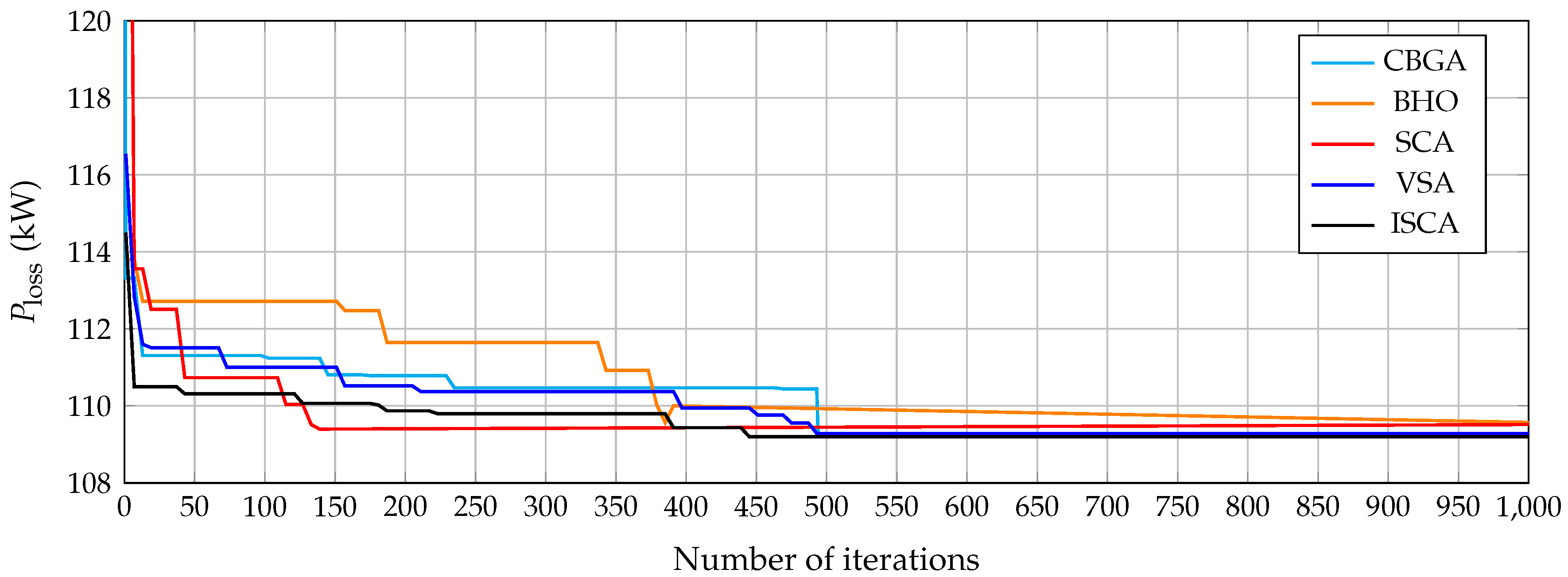
All the optimization methods required at least 50 or more individuals in the population to achieve an adequate objective function performance; the lowest minimum population size was 50, for the proposed ISCA, and the largest minimum population size was 95, for the BHO.

✓

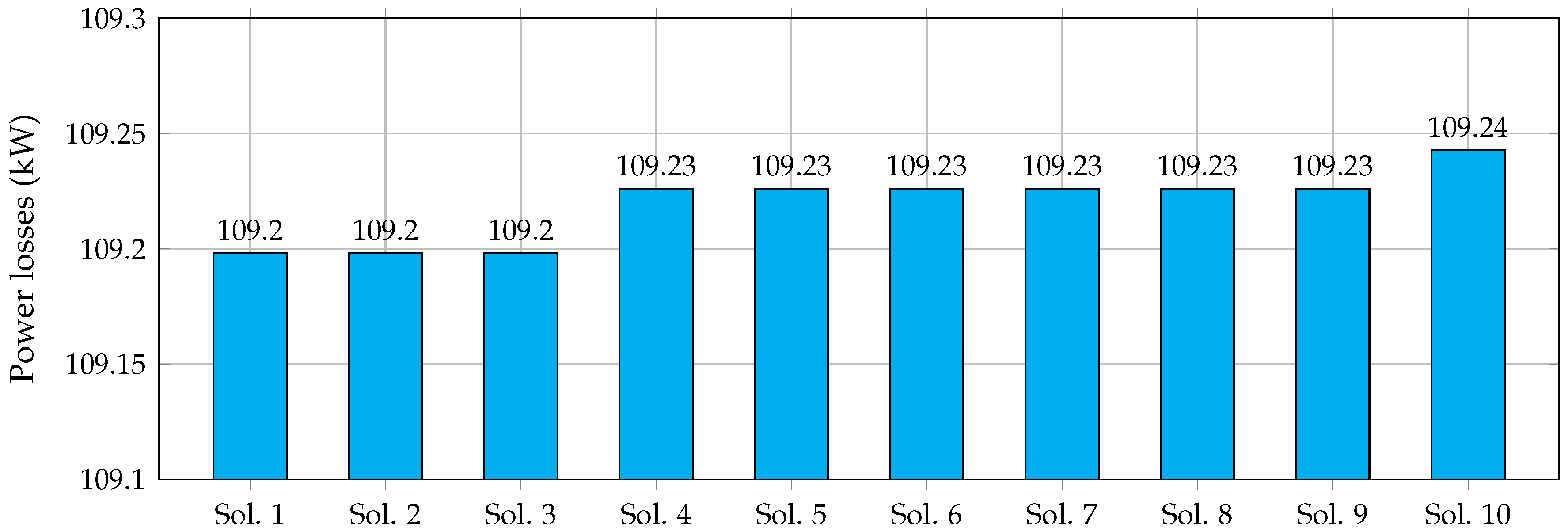
The minimum power losses were obtained by the proposed ISCA, with a value of $109.1980$ kW, followed by the CBGA with a value of $109.2218$ kW; however, the reliability of the ISCA was better since it had the lowest standard deviation of all the methods compared ($0.1144$ kW), followed by the CBGA as the second-best method with a standard deviation of about $0.2075$ kW.

✓

The ISCA presented a small variation between the extreme solutions, with a difference between the minimum and maximum values of $0.4916$ kW; the largest difference was obtained with the BHO, with a value of $3.5207$ kW. Note that the small difference between the minimum and maximum values in conjunction with the low standard deviation confirms that the ISCA obtained all the solutions inside of a small hypersphere, with the main advantage that most of the solutions obtained near to the optimal are better than the best results of the comparative methods. As an example, see the mean value of the ISCA in comparison with the minimum values of the BHO and the classical SCA.

On the other hand, to demonstrate the effectiveness of the proposed ISCA to solve the phase-balancing problem on the 15-bus system for the peak load scenario,

Table 9. Reduction of the power losses after phase balancing considering all the loads with Y-connections in the 15-bus system.

Method	Solution	Losses (kW)	Reduction (%)
Benchmark case	$\left\{1,1,1,1,1,1,1,1,1,1,1,1,1,1\right\}$	134.2472	0.00
CBGA	$\left\{3,3,4,3,5,3,3,4,3,4,5,4,3,2\right\}$	109.2218	18.64
BHO	$\left\{4,4,4,5,5,4,4,3,3,4,5,4,3,6\right\}$	109.5715	18.38
SCA	$\left\{2,1,1,5,1,2,4,2,2,2,4,6,3,4\right\}$	109.5148	18.42
VSA	$\left\{4,3,3,2,4,4,4,3,3,2,4,6,2,1\right\}$	109.2855	18.59
ISCA	$\left\{3,3,4,3,5,3,3,4,3,4,5,4,3,2\right\}$	109.1980	18.66

presents all the numerical results for all the optimization algorithms after 100 consecutive iterations, with the optimal number of individuals in the population reported in Table 8, for a total of 1000 iterations.

The results in Table 9 indicate the following: (i) all the comparative methods reduced the power losses by more than 18%; (ii) the ISCA achieved the best solution with a reduction of $18.66\%$ regarding power losses, followed by the CBGA, with a difference of $0.02\%$; (iii) the worst-performing method was the BHO with a reduction of $18.38\%$, which implies a difference of $0.3735$ kW with respect to the solution reached by the ISCA.

Figure 4 presents the 10 best objective function values determined by the ISCA after 100 consecutive evaluations. The results in this figure indicate that the difference between the first and the tenth values is only $0.04$ kW, which implies that these 10 solutions are closer to one another. In addition, a comparison of the tenth solution (i.e., $109.2427$ kW) with the results in Table 9 reveals that this result is superior to those obtained by all the comparative methods, except CBGA, which confirms the high efficiency of our proposed ISCA regarding the reduction of power losses.

On the other hand, Figure 5 shows the general evolution of the objective function value as a function of the number of iterations for each of the comparative methods and the one proposed reported in Table 9.

The behavior of the objective function value with respect to the number of iterations depicted in Figure 5 for the different metaheuristic optimizers indicates the following: (i) all of them were stabilized by about 500 iterations, since after this number none of the optimizers presented variations in the final objective function value; (ii) after the first 200 iterations, all the optimizers reached an objective function value lower than 112 kW (i.e., a reduction of about $16.57\%$), which implies that these iterations were used to explore the solution space while the remaining iterations were used to exploit the promissory regions of the solutions space identified in the exploration stage; and (iii) the classical SCA showed a premature convergence to the local optimum when compared with the proposed ISCA, since the classical SCA did not present objective function reduction after the first 150 iterations while the ISCA reached improvements during the first 450 iterations. These demonstrate the positive effect of the hybridization with the vortex search algorithm to balance the exploration and exploitation of the solution space.

5.2. Analysis of Annual Operating Costs

The results of the evaluation of the annual operating cost of the network (considering the costs of the working groups) for the IEEE 37-bus system are reported in

Table 10. Five best solutions reported by the ISCA for the IEEE 37-bus system.

Sol. No.	Solution	${\mathit{A}}_{\mathbf{cost}}$ (USD)	${\mathit{f}}_2$ (USD),
Ben. case	$\left\{1,1,1,1,1,1,1,1,1,1,1,1,1,1,1,1,1,1,1,1,1,1,1,1,1,1,1,1,1,1,1,1,1,1,1\right\}$	43,226.9376	0
Sol. 1	$\left\{3,4,1,1,2,1,1,2,1,2,1,4,5,1,3,3,3,2,1,2,1,1,3,5,6,6,2,1,6,5,3,6,1,3,1\right\}$	37,452.5749	2200
Sol. 2	$\left\{6,6,4,1,1,1,5,1,4,2,3,1,1,2,1,3,5,4,1,5,4,1,3,1,1,3,2,1,4,2,2,1,3,2,1\right\}$	37,482.4629	2100
Sol. 3	$\left\{4,3,4,1,5,1,1,2,1,3,5,2,1,4,6,2,4,3,4,4,3,1,1,1,3,1,3,1,5,1,5,1,5,5,1\right\}$	37,519.4476	2200
Sol. 4	$\left\{4,1,1,3,4,1,3,2,1,4,1,1,1,2,4,2,2,4,2,1,4,2,3,1,6,4,3,3,1,2,1,1,1,2,1\right\}$	37,533.5646	2100
Sol. 5	$\left\{1,6,1,1,2,3,1,5,6,3,4,1,1,6,3,5,1,3,1,4,1,1,1,2,1,4,3,3,3,2,1,2,3,1,3\right\}$	37,553.2596	2100

, where the five best solutions for this system are presented.

The results in Table 10 indicate the following: (i) the optimal solution obtained by the ISCA (i.e., Solution 1) allows an annual operating cost reduction of USD 5774.3627 with respect to the benchmark case; (ii) the difference in cost between the first and the final solutions reached by the ISCA was only USD $100.6840$, which is the same amount a phase change by the working group would incur; (iii) the percentage reduction with respect to the benchmark case for all the solutions was contained between $13.36\%$ and $13.13\%$ when Solutions 1 and 5 were respectively analyzed. These amounts imply that the ISCA generally allows the annual costs of operating the network to be lowered by approximately $13\%$. This would translate into a net profit for the utility company that could increase in subsequent years because the working groups would not incur additional cost in future years; (iv) the cost of the working groups oscillated between USD 2100 and USD 2200, implying that between 21 and 22, changes in the phase configuration are needed to improve the general grid performance; and (v) the average processing time to solve the phase-balancing problem with the ISCA was approximately 220 s for all 100 consecutive evaluations of the methodology. This could be considered the minimum processing time owing to the complexity of the phase-balancing optimization problem, which for the IEEE 37-bus system has a solution space with $6^{n-1}$ dimensions (with $n=37$)—tfhat is, $1.031\times {10}^{28}$ solutions are possible.

The positive impact of the phase-balancing strategy in three-phase asymmetric networks is illustrated in Figure 6, which depicts the percentage reduction in the cost of the energy losses of the network, i.e., the reduction of component $f_1$ of the objective function defined in Equation (1).

The general conclusion based on the results in Figure 6 is that the average reduction in the costs associated with the energy loss from the network was approximately $18\%$, with a maximum of $18.45\%$ for solution 1 and $17.98\%$ for solution 5.

It is worth mentioning that the cost of the energy losses, i.e., the objective function $f_1$, had a participation about $94.1259\%$ in the total annual operative costs for Solution 1 and $94.4079\%$ in the case of Solution 5 (see Table 10). This implies that, with inversions lower than 6% of the $A_{\cos \mathrm{t}}$, it is possible to reach important reductions in the amount of grid power losses and their costs, as presented in Figure 6. This is indeed the most important component of the objective function in the case of the IEEE 37-bus system.

The numerical values in Figure 7 indicate that phases a and c involved reductions of $126.98$ kWh/day and $408.17$ kWh/day regarding the daily energy losses, respectively, whereas phase c experienced an increase of $220.80$ kWh/day. This behavior is expected in the phases of the network because the objective of the phase-balancing problem is to reduce the level of asymmetry of the network, which is then achieved by redistributing all the loads of the network as uniformly as possible. Note that even if the daily energy losses of phase b were to increase, the general effect of phase balancing is a global daily reduction of $314.35$ kWh/day or $18.45\%$, as presented in Figure 4 for Solution 1.

In addition, to observe the benefit derived from the reduction in the energy losses in terms of the general electrical performance of the system, we present the total daily energy losses per phase for the benchmark case and for the best solution produced by the proposed ISCA in Figure 7.

5.3. Complementary Analysis

Here, we present some additional results and comments for the IEEE 37-bus system that allow us to confirm the positive effects that allow the implementation of the phase-balancing plan through the working groups along the grid. One of the most significant effects of the phase-balancing in three-phase asymmetric networks was the general improvement of the voltage profile in all nodes of the network. Figure 8 presents the general performance of the voltage profile before and after implementing the phase-balancing plan in Solution 1 (see Table 10).

The behavior of the voltage profiles in Figure 8 indicates the following: (i) Some magnitudes of the voltages in phases a and c had a regulation voltage higher than 5%, namely, nodes 13 to 22 with voltages lower than 0.95 p.u. (Figure 8a). (ii) Phase b showed a better voltage performance in the benchmark case (see Figure 8a) when compared to phases a and c, which is an expected behavior since this phase had lower active and reactive power demand consumption when compared with the other phases. The active and reactive power consumption in all the phases were 727 kW and 357 kvar for phase a, 639 kW and 314 kvar for phase b, and 1091 kW and 530 kvar for phase c. (iii) After the implementation of the phase-balancing plan (i.e., Solution 1 in Table 10), all the phases had a maximum voltage regulation of 4%, which implies that all the voltage profiles were above or equal to 0.96 p.u. In addition, all the phases presented a closer voltage behavior, which is the product of the load redistribution in all the phases, which had the following final consumptions: 763 kW and 371 kvar for phase a; 941 kW and 461 kvar for phase b; and 753 kW and 369 kvar for phase c.

An additional important result after implementing the phase-balancing plan is the improvement of the general grade of unbalance of the network. The grade of unbalance was measured for each phase with respect to the ideal consumption of the phase (perfectly balanced case), which was obtained through the average of the active and reactive power consumption in all of the phases. The ideal active and reactive power consumptions for the IEEE 37-bus system would be 819 kW and 400.33 kvar. With these values, the grades of unbalance before and after the implementation of the phase-balancing plan are reported in

Table 11. Grade of unbalance in the IEEE 37-bus system before and after implementing the phase-balancing plan.

Benchmark Case			Solution 1
Phase	Unb. Active (%)	Unb. Reactive (%)	Phase	Unb. Active (%)	Unb. Reactive (%)
a	11.2332	10.8243	a	6.8376	7.3272
b	21.9780	21.5654	b	14.8962	15.1540
c	33.2112	32.3897	c	8.0586	7.8268

.

The results in Table 11 show the following: (i) Phase c had the highest level of unbalance with respect to the ideal case in the benchmark scenario (greater than 30% for active and reactive power demands); this was because this phase had the highest demand in this scenario, with 1091 kW and 530 kvar (i.e., with an additional 272 kW and 129.67 kvar with respect to the ideal case). (ii) After implementing the phase-balancing plan, the highest level of unbalance corresponding to phase b was about $14.90\%$ for the active power and $15.15\%$ for the reactive power. (iii) Phases a and c reduced their active and reactive power unbalances from two digits to one digit, beginning their variation in phase c with more than 25% in both power demands.

Regarding the implementation of the phase-balancing plan by part of the working groups, it is important to mention that only a few trained staff with the ability to disconnect and reconnect transformers at the point of common coupling between the loads and the distribution feeder are required. However, before making any physical interventions in the network that will affect the electricity supply, the utility staff must follow the norms of each country regarding the notification of the end-users.

6. Conclusions

The problem of optimal phase balancing in three-phase asymmetric distribution networks was addressed in this research. The problem was solved from the point of view of metaheuristic optimization using a newly proposed master–slave optimization approach. The master stage employs an improved version of the sine cosine algorithm to determine the load connections among phases by using integer codification. In the slave stage, the triangular-based power flow method is used for three-phase networks that operate with loads with Y- and $\Delta$-connections. Two test feeders composed of 15 and 37 nodes were employed for the numerical validation of the proposed ISCA to solve the phase-balancing problem.

The numerical results for the 15-bus system demonstrated that the ISCA allowed a total power loss reduction of $18.66\%$ with respect to the benchmark case. These results were superior to those of the genetic algorithm ($18.64\%$), black hole optimizer ($18.04\%$), sine cosine algorithm ($18.51\%$), and vortex search algorithm ($18.57\%$). In addition, the difference in power losses among the 10 best solutions reached by the proposed ISCA was approximately $0.04$ kW, demonstrating its efficiency with respect to solving the phase-balancing problem in three-phase asymmetric networks.

The computational validations of the IEEE 37-bus system demonstrated that the proposed ISCA allowed reductions of approximately $13\%$ in the annual operating costs of the network, with investments between USD 2100 and USD $2200$ in working groups to implement the optimal phase-balancing plan along the test feeder in nodes where changes are required. In addition, the voltage regulation in the IEEE 37-bus system was improved from 6.3% to 4% when compared to the benchmark case with the implementation of the phase-balancing plan. In addition, the average processing time to solve the optimization problem was approximately 220 s, which can be considered a relatively small computational requirement, given that the dimension of the solution space for the IEEE 37-bus system is higher than $1\times {10}^{28}$.

In the future, the following research aims should be addressed: (i) to use the proposed ISCA to solve the problem of the optimal selection of conductors for three-phase asymmetric networks, including the phase-balancing strategy in a unique codification; and (ii) to propose a convex programming model that allows the global optimal solution of the phase-balancing problem to be reached using conic programming, and to compare these results with those of the proposed ISCA to determine the discrepancy between the global optimal solution and the solutions reached using metaheuristics.

References

1. Cheng, L.; Chang, Y.; Liu, M.; Feng, H.; Wu, Q. Typical medium voltage distribution system topologies in China: A review and a comparison of reliability. In Proceedings of the 2014 International Conference on Probabilistic Methods Applied to Power Systems (PMAPS), Durham, UK, 7 July 2014; IEEE: Piscataway, NJ, USA, 2014. [Google Scholar] [CrossRef]
2. Temiz, A.; Almalki, A.M.; Kahraman, Ö.; Alshahrani, S.S.; Sönmez, E.B.; Almutairi, S.S.; Nadar, A.; Smiai, M.S.; Alabduljabbar, A.A. Investigation of MV Distribution Networks with High-Penetration Distributed PVs: Study for an Urban Area. Energy Procedia 2017, 141, 517–524. [Google Scholar] [CrossRef]
3. Zamani, A.; Sidhu, T.; Yazdani, A. A strategy for protection coordination in radial distribution networks with distributed generators. In Proceedings of the IEEE PES General Meeting, Minneapolis, MN, USA, 25–29 July 2010; IEEE: Piscataway, NJ, USA, 2010. [Google Scholar] [CrossRef]
4. Zhu, J.; Bilbro, G.; Chow, M.Y. Phase balancing using simulated annealing. IEEE Trans. Power Syst. 1999, 14, 1508–1513. [Google Scholar] [CrossRef] [Green Version]
5. Cortés-Caicedo, B.; Avellaneda-Gómez, L.S.; Montoya, O.D.; Alvarado-Barrios, L.; Chamorro, H.R. Application of the Vortex Search Algorithm to the Phase-Balancing Problem in Distribution Systems. Energies 2021, 14, 1282. [Google Scholar] [CrossRef]
6. Riaño, F.E.; Cruz, J.F.; Montoya, O.D.; Chamorro, H.R.; Alvarado-Barrios, L. Reduction of Losses and Operating Costs in Distribution Networks Using a Genetic Algorithm and Mathematical Optimization. Electronics 2021, 10, 419. [Google Scholar] [CrossRef]
7. Soma, G.G. Optimal Sizing and Placement of Capacitor Banks in Distribution Networks Using a Genetic Algorithm. Electricity 2021, 2, 187–204. [Google Scholar] [CrossRef]
8. Gil-González, W.; Montoya, O.D.; Rajagopalan, A.; Grisales-Noreña, L.F.; Hernández, J.C. Optimal Selection and Location of Fixed-Step Capacitor Banks in Distribution Networks Using a Discrete Version of the Vortex Search Algorithm. Energies 2020, 13, 4914. [Google Scholar] [CrossRef]
9. Lueken, C.; Carvalho, P.M.; Apt, J. Distribution grid reconfiguration reduces power losses and helps integrate renewables. Energy Policy 2012, 48, 260–273. [Google Scholar] [CrossRef]
10. Vai, V.; Suk, S.; Lorm, R.; Chhlonh, C.; Eng, S.; Bun, L. Optimal Reconfiguration in Distribution Systems with Distributed Generations Based on Modified Sequential Switch Opening and Exchange. Appl. Sci. 2021, 11, 2146. [Google Scholar] [CrossRef]
11. Granada-Echeverri, M.; Gallego-Rendón, R.A.; López-Lezama, J.M. Optimal Phase Balancing Planning for Loss Reduction in Distribution Systems using a Specialized Genetic Algorithm. Ingeniería Cienc. 2012, 8, 121–140. [Google Scholar] [CrossRef] [Green Version]
12. Huang, M.Y.; Chen, C.S.; Lin, C.H.; Kang, M.S.; Chuang, H.J.; Huang, C.W. Three-phase balancing of distribution feeders using immune algorithm. IET Gener. Transm. Distrib. 2008, 2, 383. [Google Scholar] [CrossRef]
13. Montoya, O.D.; Gil-González, W.; Hernández, J.C. Efficient Operative Cost Reduction in Distribution Grids Considering the Optimal Placement and Sizing of D-STATCOMs Using a Discrete-Continuous VSA. Appl. Sci. 2021, 11, 2175. [Google Scholar] [CrossRef]
14. Kong, W.; Ma, K.; Fang, L.; Wei, R.; Li, F. Cost-Benefit Analysis of Phase Balancing Solution for Data-Scarce LV Networks by Cluster-Wise Gaussian Process Regression. IEEE Trans. Power Syst. 2020, 35, 3170–3180. [Google Scholar] [CrossRef]
15. Han, X.; Wang, H.; Liang, D. Master-slave game optimization method of smart energy systems considering the uncertainty of renewable energy. Int. J. Energy Res. 2020, 45, 642–660. [Google Scholar] [CrossRef]
16. Montoya, O.D.; Molina-Cabrera, A.; Grisales-Noreña, L.F.; Hincapié, R.A.; Granada, M. Improved Genetic Algorithm for Phase-Balancing in Three-Phase Distribution Networks: A Master-Slave Optimization Approach. Computation 2021, 9, 67. [Google Scholar] [CrossRef]
17. Fei, C.-G.; Wang, R. Using Phase Swapping to Solve Load Phase Balancing by ADSCHNN in LV Distribution Network. Int. J. Control Autom. 2014, 7, 1–14. [Google Scholar] [CrossRef]
18. Siti, M.; Jimoh, A.; Nicolae, D. Phase load balancing in the secondary distribution network using fuzzy logic. In Proceedings of the AFRICON 2007, Windhoek, Namibia, 26–28 September 2007; IEEE: Piscataway, NJ, USA, 2007. [Google Scholar] [CrossRef]
19. Sathiskumar, M.; kumar, A.N.; Lakshminarasimman, L.; Thiruvenkadam, S. A self adaptive hybrid differential evolution algorithm for phase balancing of unbalanced distribution system. Int. J. Electr. Power Energy Syst. 2012, 42, 91–97. [Google Scholar] [CrossRef]
20. Hooshmand, R.A.; Soltani, S. Fuzzy Optimal Phase Balancing of Radial and Meshed Distribution Networks Using BF-PSO Algorithm. IEEE Trans. Power Syst. 2012, 27, 47–57. [Google Scholar] [CrossRef]
21. Hooshmand, R.; Soltani, S. Simultaneous optimization of phase balancing and reconfiguration in distribution networks using BF–NM algorithm. Int. J. Electr. Power Energy Syst. 2012, 41, 76–86. [Google Scholar] [CrossRef]
22. Garces, A.; Gil-González, W.; Montoya, O.D.; Chamorro, H.R.; Alvarado-Barrios, L. A Mixed-Integer Quadratic Formulation of the Phase-Balancing Problem in Residential Microgrids. Appl. Sci. 2021, 11, 1972. [Google Scholar] [CrossRef]
23. Montoya, O.D.; Arias-Londoño, A.; Grisales-Noreña, L.F.; Barrios, J.Á.; Chamorro, H.R. Optimal Demand Reconfiguration in Three-Phase Distribution Grids Using an MI-Convex Model. Symmetry 2021, 13, 1124. [Google Scholar] [CrossRef]
24. Khodr, H.; Zerpa, I.; de Jesu’s, P.D.O.; Matos, M. Optimal Phase Balancing in Distribution System Using Mixed-Integer Linear Programming. In Proceedings of the 2006 IEEE/PES Transmission & Distribution Conference and Exposition: Latin America, Caracas, Venezuela, 15–18 August 2006; IEEE: Piscataway, NJ, USA, 2006. [Google Scholar] [CrossRef]
25. Turgut, M.S.; Turgut, O.E.; Afan, H.A.; El-Shafie, A. A novel Master–Slave optimization algorithm for generating an optimal release policy in case of reservoir operation. J. Hydrol. 2019, 577, 123959. [Google Scholar] [CrossRef]
26. Yang, B.; Chen, Y.; Zhao, Z.; Han, Q. A Master-Slave Particle Swarm Optimization Algorithm for Solving Constrained Optimization Problems. In Proceedings of the 2006 6th World Congress on Intelligent Control and Automation, Dalian, China, 21–23 June 2006; IEEE: Piscataway, NJ, USA, 2006. [Google Scholar] [CrossRef]
27. Jesus, P.D.O.D.; Alvarez, M.; Yusta, J. Distribution power flow method based on a real quasi-symmetric matrix. Electr. Power Syst. Res. 2013, 95, 148–159. [Google Scholar] [CrossRef]
28. Montoya, O.D.; Giraldo, J.S.; Grisales-Noreña, L.F.; Chamorro, H.R.; Alvarado-Barrios, L. Accurate and Efficient Derivative-Free Three-Phase Power Flow Method for Unbalanced Distribution Networks. Computation 2021, 9, 61. [Google Scholar] [CrossRef]
29. Naumov, I.V.; Karamov, D.N.; Tretyakov, A.N.; Yakupova, M.A.; Fedorinova, E.S. Asymmetric power consumption in rural electric networks. In Proceedings of the IOP Conference Series: Earth and Environmental Science 2021, Kuala Lumpur, Malaysia, 16 April 2021; Volume 677, p. 032088. [Google Scholar] [CrossRef]
30. Hu, R.; Li, Q.; Qiu, F. Ensemble Learning Based Convex Approximation of Three-Phase Power Flow. IEEE Trans. Power Syst. 2021, 1–10. [Google Scholar] [CrossRef]
31. Shen, T.; Li, Y.; Xiang, J. A Graph-Based Power Flow Method for Balanced Distribution Systems. Energies 2018, 11, 511. [Google Scholar] [CrossRef] [Green Version]
32. Marini, A.; Mortazavi, S.; Piegari, L.; Ghazizadeh, M.S. An efficient graph-based power flow algorithm for electrical distribution systems with a comprehensive modeling of distributed generations. Electr. Power Syst. Res. 2019, 170, 229–243. [Google Scholar] [CrossRef]
33. Montoya, O.D.; Molina-Cabrera, A.; Chamorro, H.R.; Alvarado-Barrios, L.; Rivas-Trujillo, E. A Hybrid Approach Based on SOCP and the Discrete Version of the SCA for Optimal Placement and Sizing DGs in AC Distribution Networks. Electronics 2020, 10, 26. [Google Scholar] [CrossRef]
34. Mirjalili, S. SCA: A Sine Cosine Algorithm for solving optimization problems. Knowl. Based Syst. 2016, 96, 120–133. [Google Scholar] [CrossRef]
35. Herrera-Briñez, M.C.; Montoya, O.D.; Alvarado-Barrios, L.; Chamorro, H.R. The Equivalence between Successive Approximations and Matricial Load Flow Formulations. Appl. Sci. 2021, 11, 2905. [Google Scholar] [CrossRef]
36. Montoya, O.D.; Gil-González, W.; Grisales-Noreña, L.; Orozco-Henao, C.; Serra, F. Economic Dispatch of BESS and Renewable Generators in DC Microgrids Using Voltage-Dependent Load Models. Energies 2019, 12, 4494. [Google Scholar] [CrossRef] [Green Version]
37. Attia, A.F.; Sehiemy, R.A.E.; Hasanien, H.M. Optimal power flow solution in power systems using a novel Sine-Cosine algorithm. Int. J. Electr. Power Energy Syst. 2018, 99, 331–343. [Google Scholar] [CrossRef]
38. Hasan, Z.; El-Hawary, M.E. Optimal Power Flow by Black Hole Optimization Algorithm. In Proceedings of the 2014 IEEE Electrical Power and Energy Conference, Calgary, AB, Canada, 12–14 November 2014; IEEE: Piscataway, NJ, USA, 2014. [Google Scholar] [CrossRef]
Figure 1. Nodal connections among nodes in the 15-bus system.
Energies 14 04535 g001
Figure 2. Connections among nodes in the IEEE 37-bus system.
Energies 14 04535 g002
Figure 3. Typical active and reactive power consumption curves in Colombia [13].
Energies 14 04535 g003
Figure 4. Ten best solutions reached by the proposed ISCA for the 15-bus system.
Energies 14 04535 g004
Figure 5. Evolution of the objective function value for the 15-bus system with different metaheuristic optimizers.
Energies 14 04535 g005
Figure 6. Level of reduction in the energy losses for the five best solutions reached by the ISCA for the IEEE 37-bus system.
Energies 14 04535 g006
Figure 7. Daily energy losses per phase before and after using the proposed ISCA for optimal phase-balancing in the IEEE 37-bus system.
Energies 14 04535 g007
Figure 8. Performance of the voltage profiles in the IEEE 37-bus system: (a) benchmark simulation scenario, and (b) after implementing the phase-balancing plan in Solution 1.
Energies 14 04535 g008