
Novel District Heating Systems: Methods and Simulation Results †

 , , , ,
Abstract
:1. Introduction
1.1. State of the Art Tools
1.2. Scope and Limitaions
2. Methodology
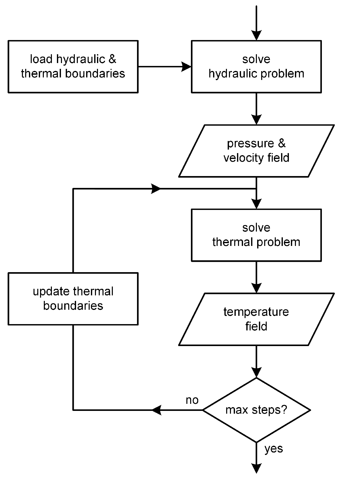
2.1. Thermohydraulic Simulation
2.2. Pipe Network
2.2.1. Hydraulic Calculation
2.2.2. Thermal Calculation
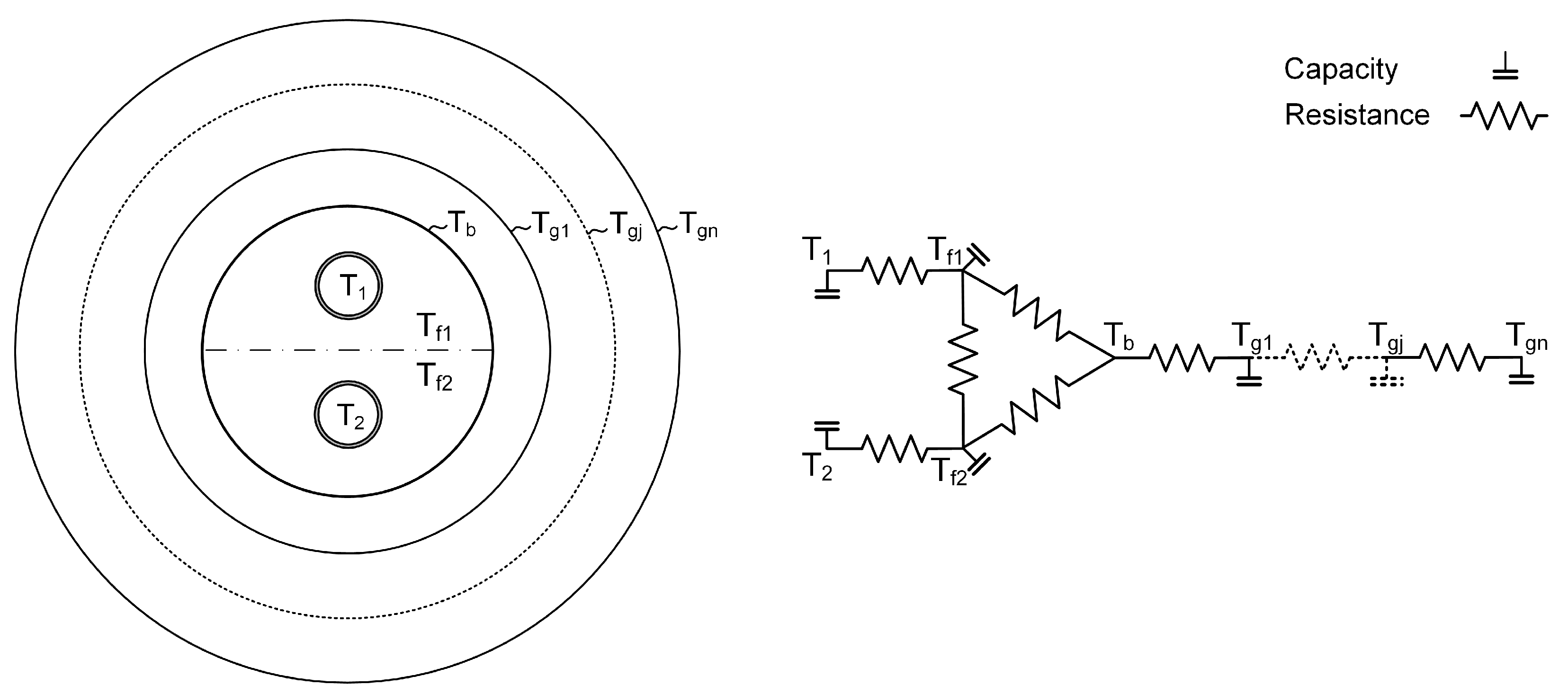
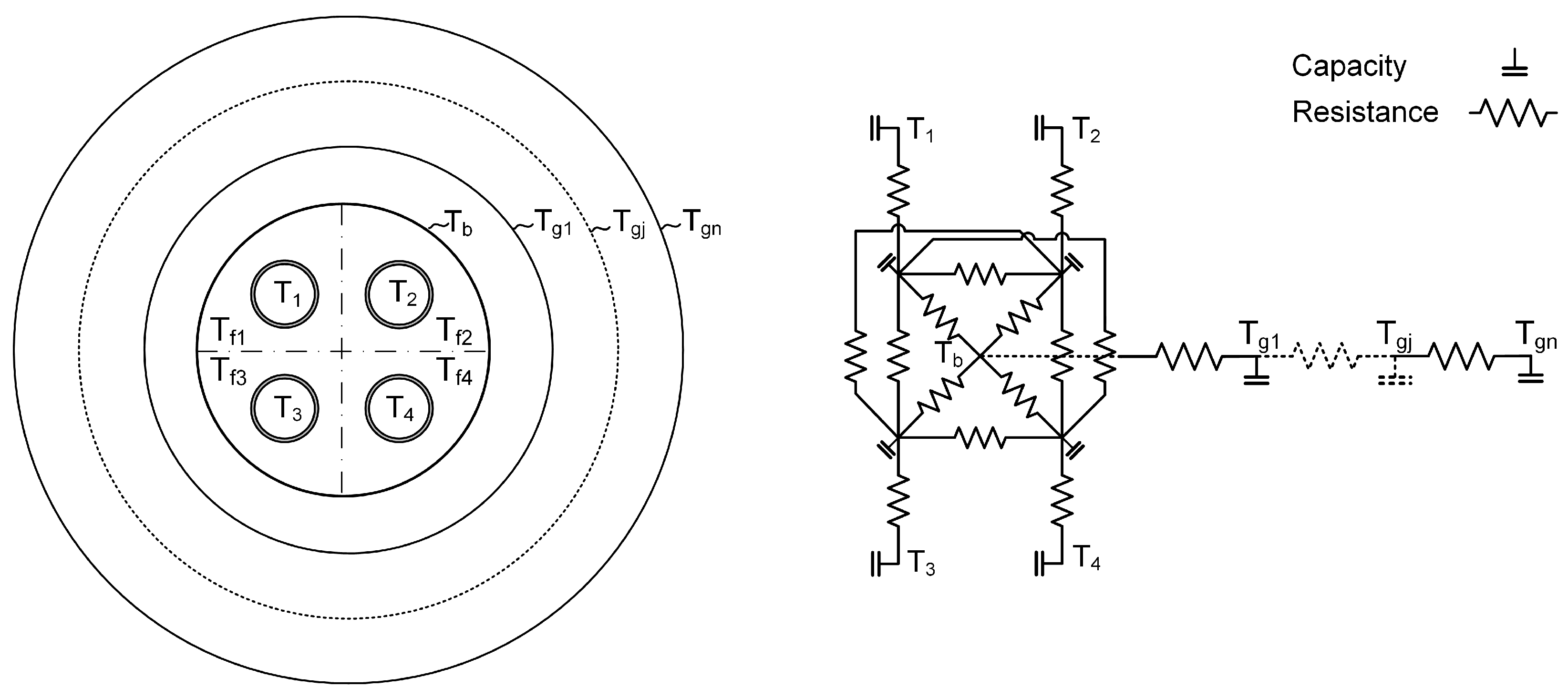
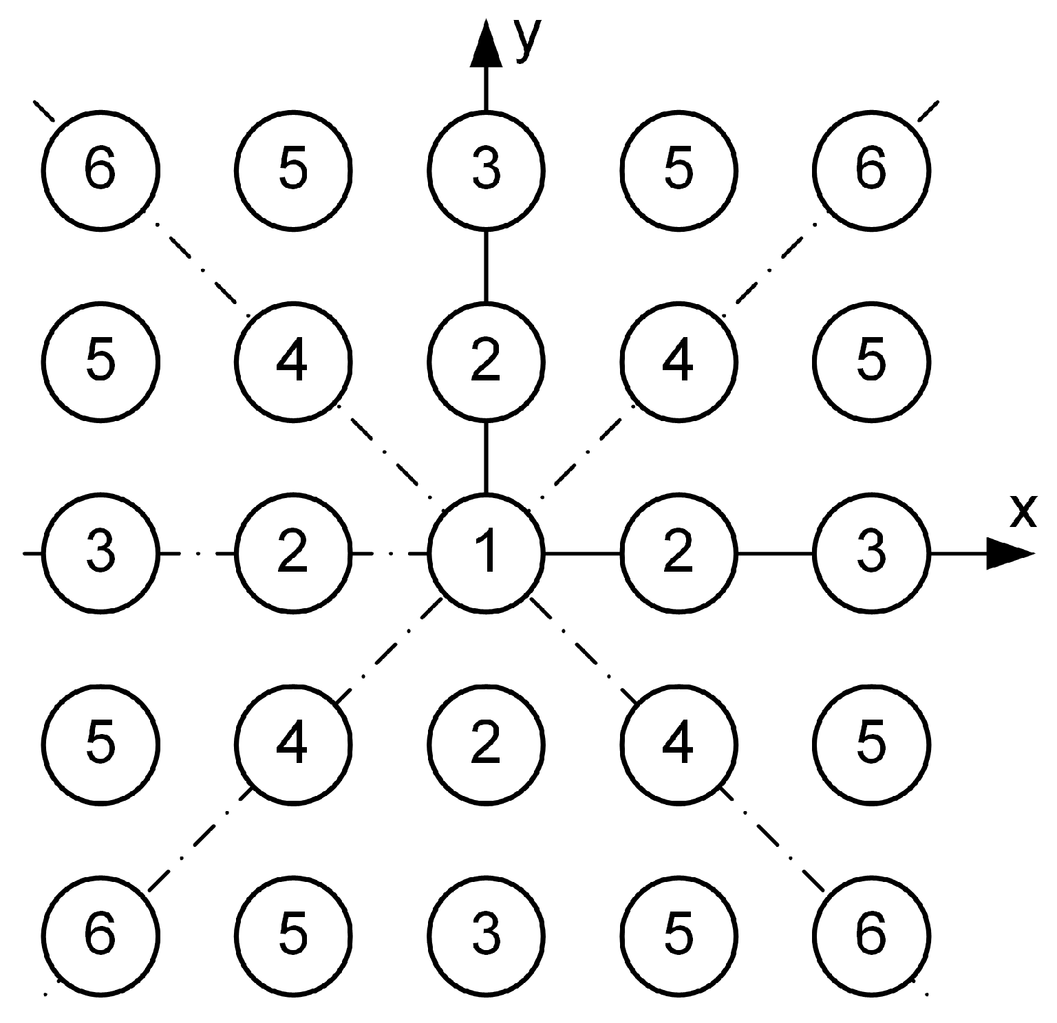
2.3. BTES
2.3.1. Hydraulic Calculation
2.3.2. Thermal Calculation
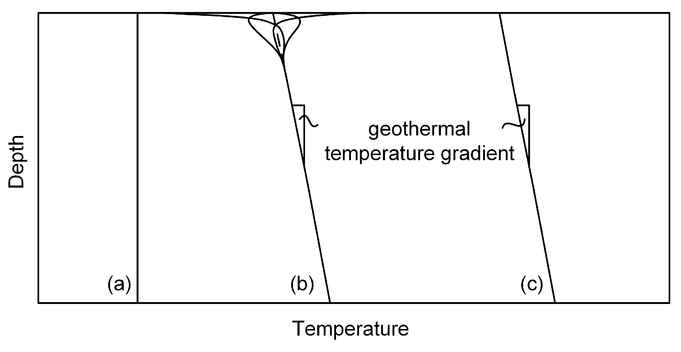
2.4. Boundary Conditions
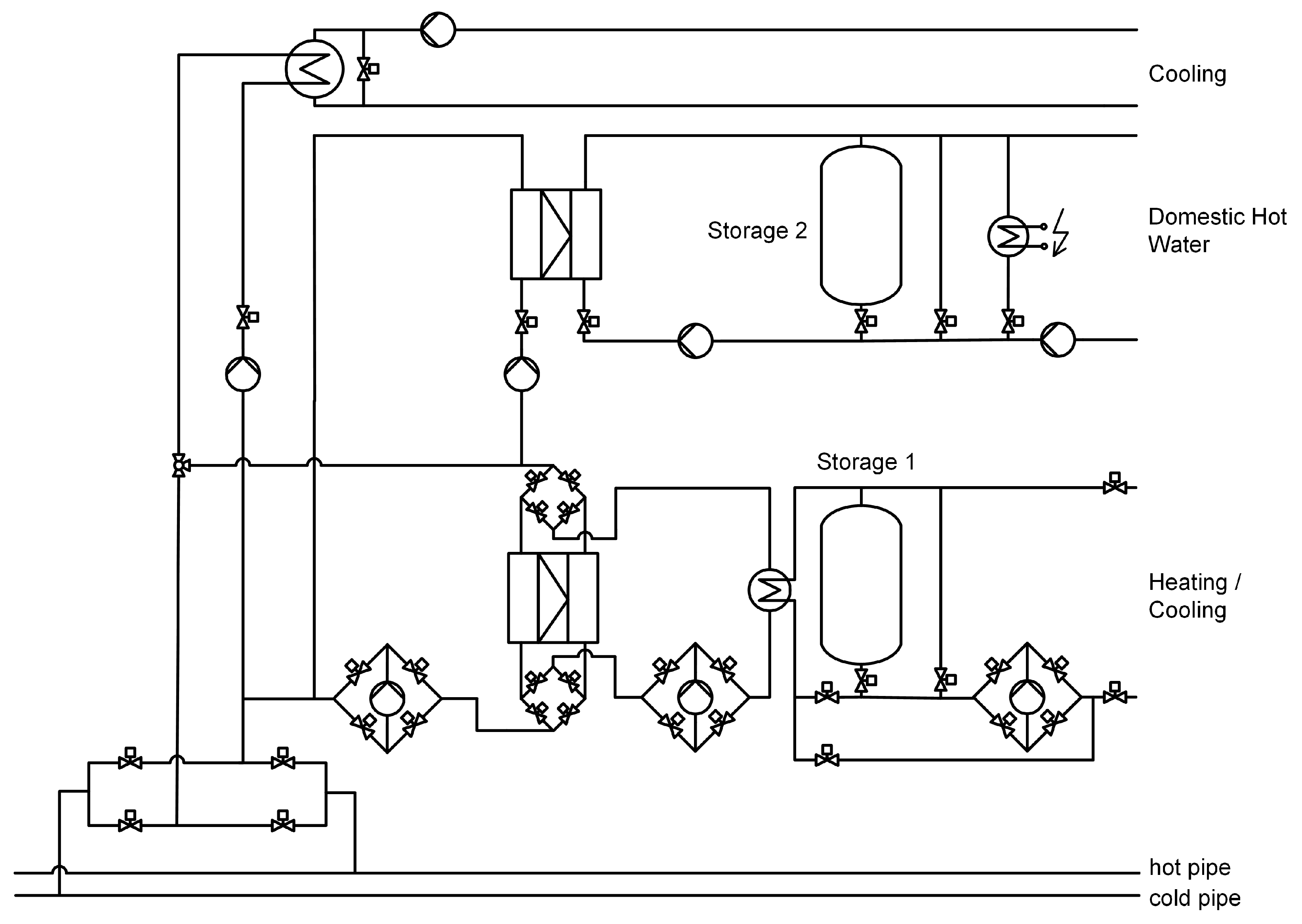
2.5. Energy Transfer Stations
- Supply of hot water for H;
- Supply of hot water for DHW;
- Supply of cold water for FC or AC.
2.5.1. Heat Pumps
2.5.2. Heat Exchangers
2.5.3. Short Term Water Storages
2.5.4. Circulation Pumps
3. Validation
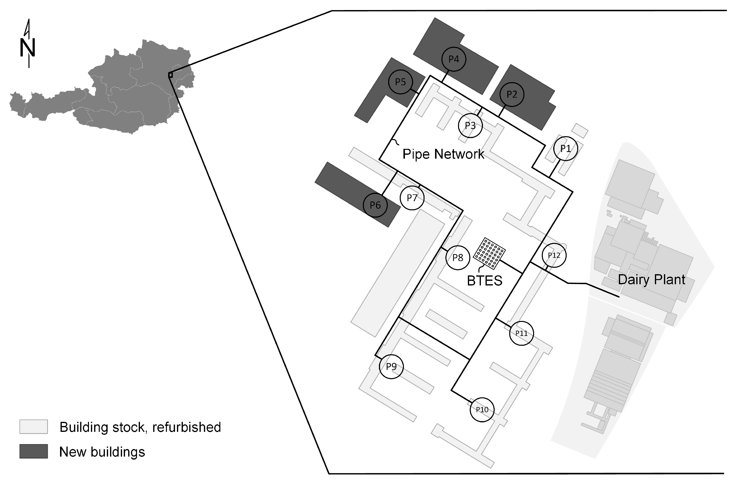
4. Use Case
4.1. System Design and Heat Input
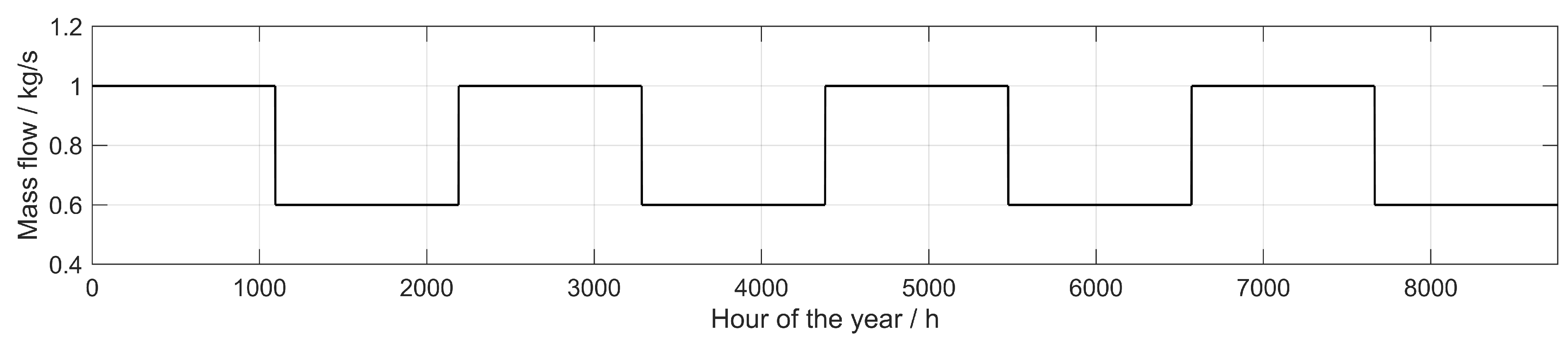
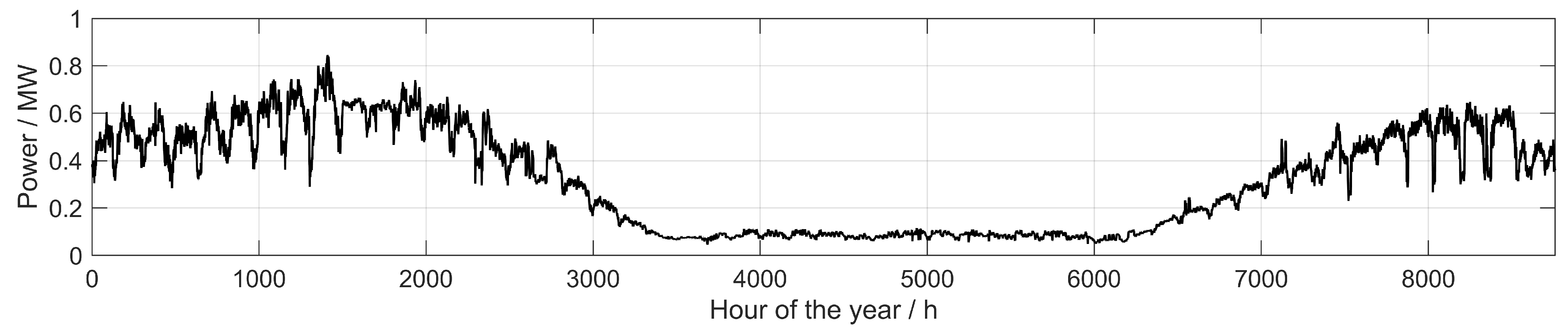
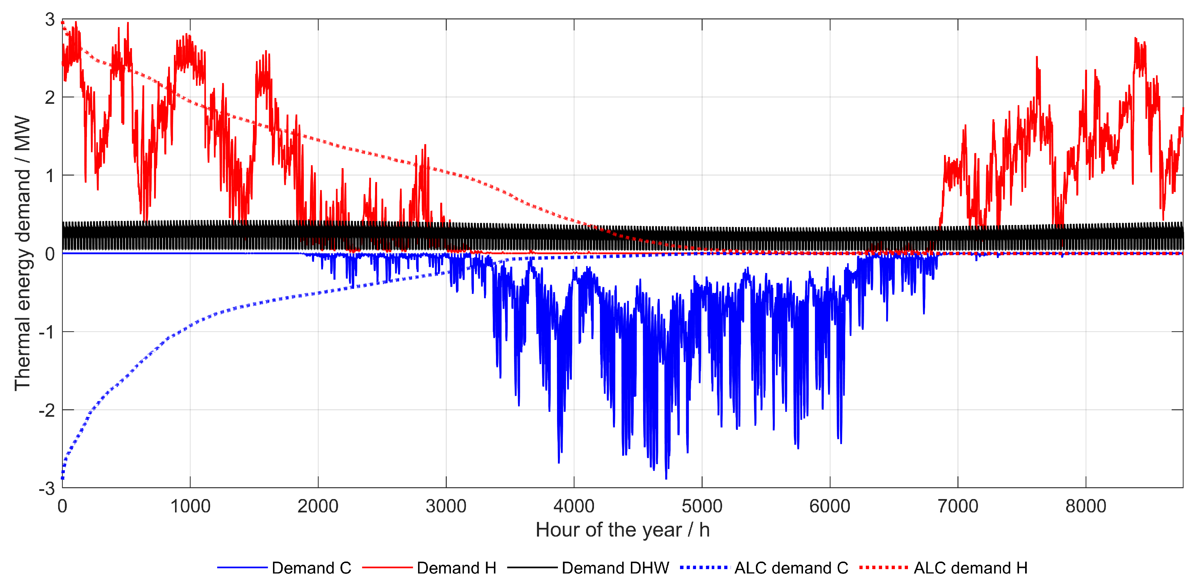
4.2. Energy Demand
5. Results and Discussion
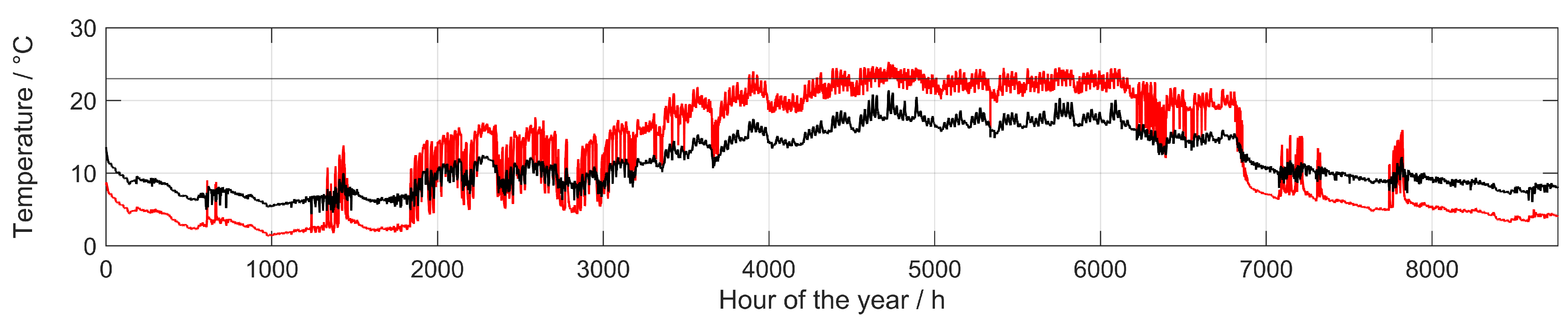
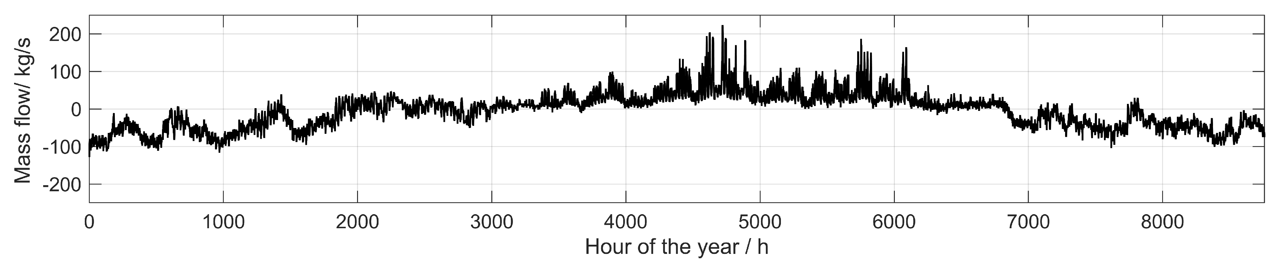
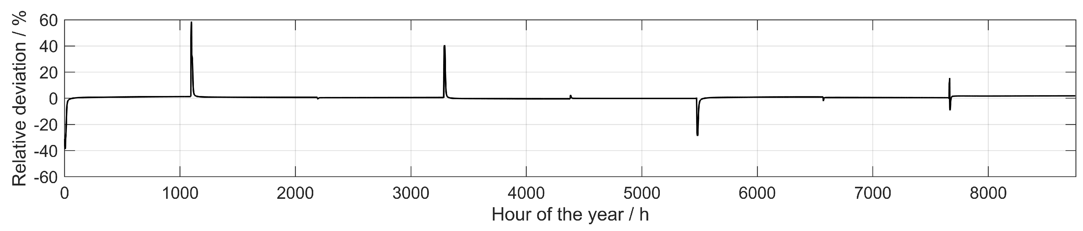
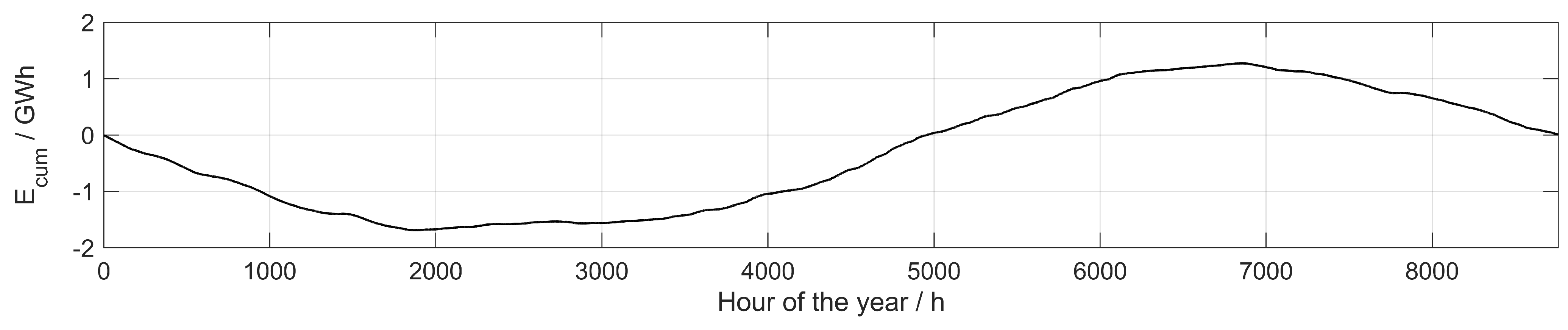
5.1. Dynamic Behavior BTES
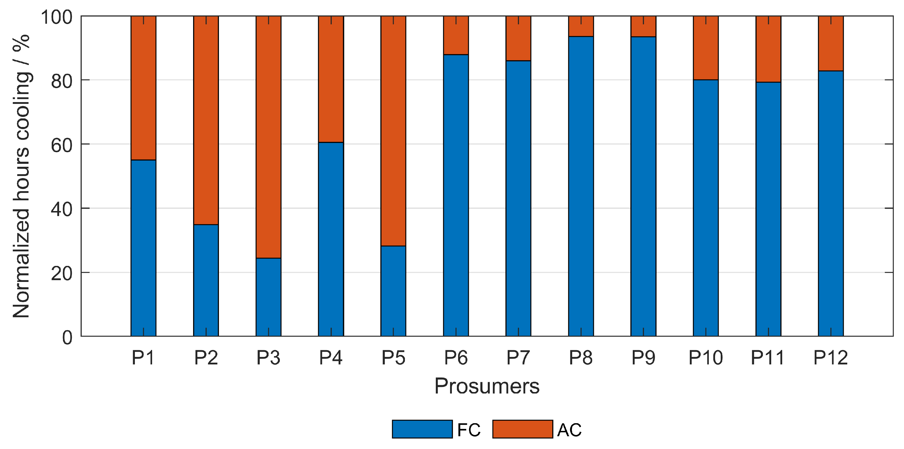
5.2. Share of AC and FC
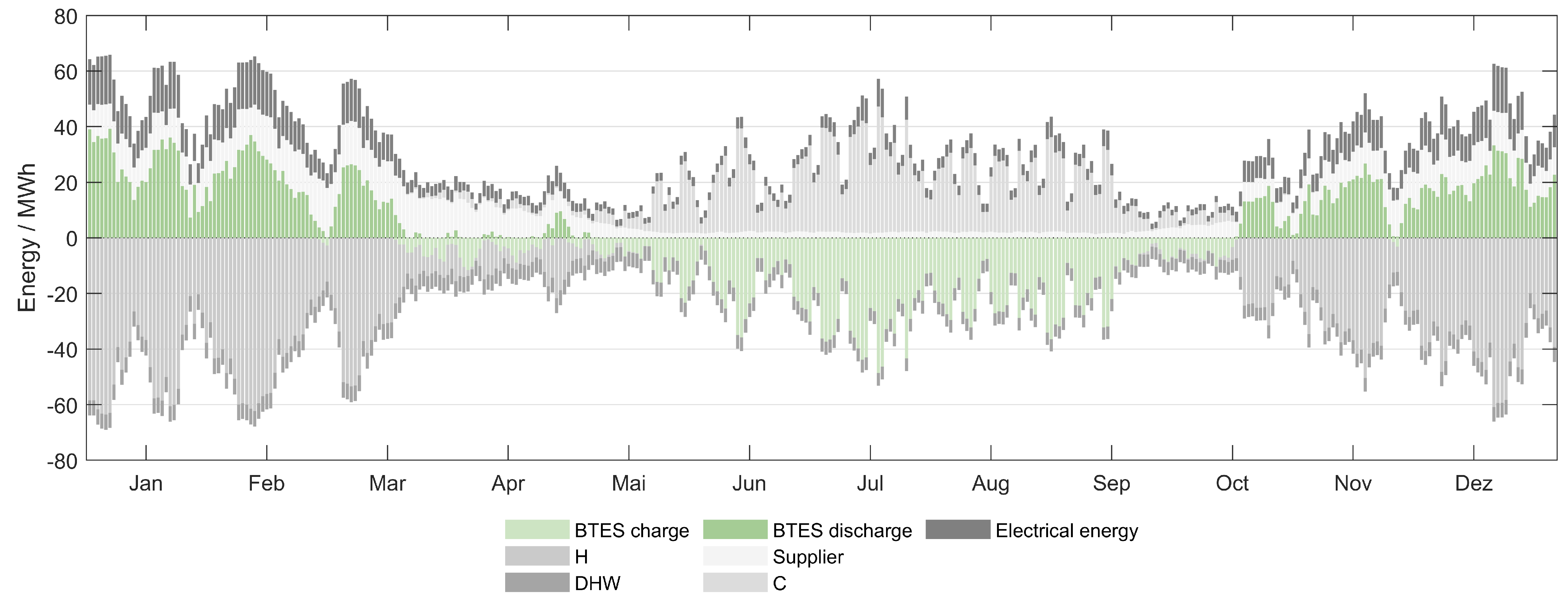
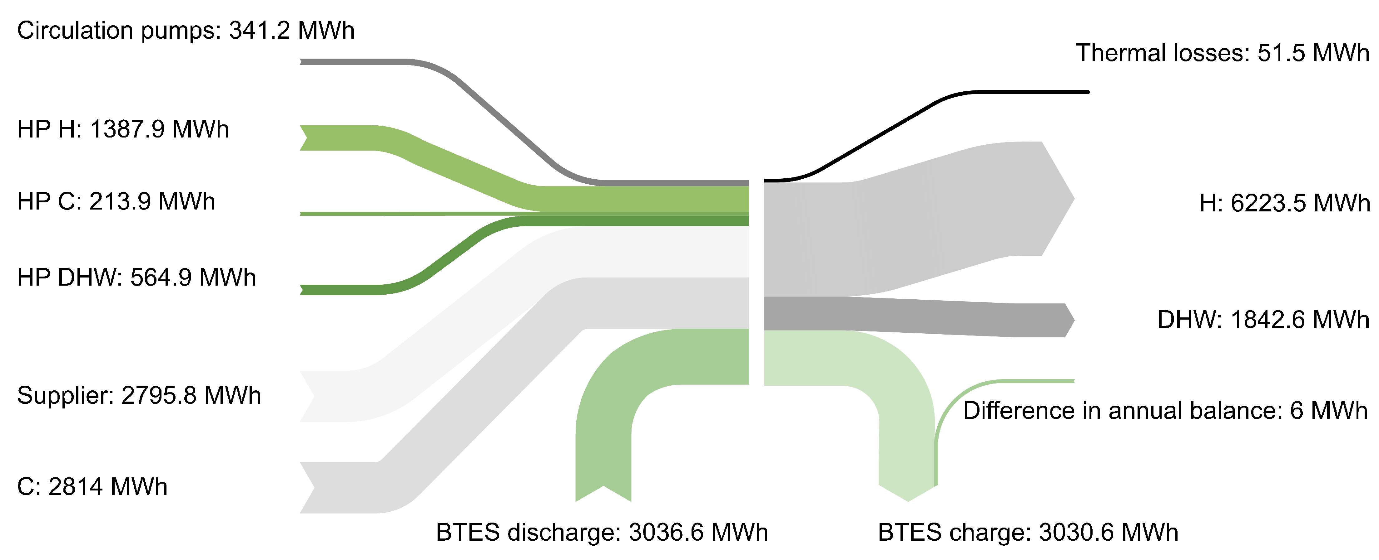
5.3. Energy Flows
6. Conclusions
Author Contributions
Funding
Institutional Review Board Statement
Informed Consent Statement
Data Availability Statement
Acknowledgments
Conflicts of Interest
Abbreviations
| AC | Active Cooling |
| BTES | Borehole Thermal Energy Storage |
| C | Cooling |
| COP | Coefficient of Performance |
| DHC | Distric Heating and Cooling |
| DHW | Domestic Hot Water |
| ETS | Energy Transfer Station |
| FC | Free Cooling |
| GFA | Gross Floor Area |
| H | Heating |
| HP | Heat Pump |
| RCM | Thermal Resistance and Capacity Model |
| SANBA | Smart Anergy Quarter Baden |
| TEGSim | Thermal Energy Grid Simulation |
| TRY | Test Reference Year |
| ULTDH | Ultra-Low-Temperature District Heating |
References
- Statistik Austria–Direktion Raumwirtschaft. Nutzenergieanalyse für Österreich 1993–2019. Available online: http://www.statistik.at/web_de/statistiken/energie_umwelt_innovation_mobilitaet/energie_und_umwelt/energie/nutzenergieanalyse/index.html (accessed on 10 January 2021).
- Aus Verantwortung für Österreich. Regierungsprogramm 2020–2024. Available online: https://www.bundeskanzleramt.gv.at/bundeskanzleramt/die-bundesregierung/regierungsdokumente.html (accessed on 14 January 2021).
- Rezaie, B.; Rosen, M.A. District heating and cooling: Review of technology and potential enhancements. Appl. Energy 2012, 93, 2–10. [Google Scholar] [CrossRef]
- Duquette, J.; Rowe, A.; Wild, P. Thermal performance of a steady state physical pipe model for simulating district heating grids with variable flow. Appl. Energy 2016, 178, 383–393. [Google Scholar] [CrossRef]
- Boesten, S.; Ivens, W.; Dekker, S.C.; Eijdems, H. 5th generation district heating and cooling systems as a solution for renewable urban thermal energy supply. Adv. Geosci. 2019, 49, 129–136. [Google Scholar] [CrossRef] [Green Version]
- Lund, H.; Werner, S.; Wiltshire, R.; Svendsen, S.; Thorsen, J.E.; Hvelplund, F.; Mathiesen, B.V. 4th Generation District Heating (4GDH). Energy 2014, 68, 1–11. [Google Scholar] [CrossRef]
- Lund, H.; Østergaard, P.A.; Chang, M.; Werner, S.; Svendsen, S.; Sorknæs, P.; Thorsen, J.E.; Hvelplund, F.; Mortensen, B.O.G.; Mathiesen, B.V.; et al. The status of 4th generation district heating: Research and results. Energy 2018, 164, 147–159. [Google Scholar] [CrossRef]
- Sanner, B. (Ed.) Common Vision for the Renewable Heating & Cooling Sector in Europe; Office of the European Union: Luxemburg, 2011. [Google Scholar]
- Buffa, S.; Cozzini, M.; D’Antoni, M.; Baratieri, M.; Fedrizzi, R. 5th generation district heating and cooling systems: A review of existing cases in Europe. Renew. Sustain. Energy Rev. 2019, 104, 504–522. [Google Scholar] [CrossRef]
- Gabrielli, P.; Acquilino, A.; Siri, S.; Bracco, S.; Sansavini, G.; Mazzotti, M. Optimization of low-carbon multi-energy systems with seasonal geothermal energy storage: The Anergy Grid of ETH Zurich. Energy Convers. Manag. X 2020, 8, 100052. [Google Scholar] [CrossRef]
- Fuchsluger, M.; Götzl, G.; Steiner, C.; Weilbold, J.; Rupprecht, D.; Kessler, T.; Heimlich, K.; Ponweiser, K.; Nagler, J.; Bothe, D.; et al. DEGENT-NET Dezentrale Geothermale Niedertemperatur-Wärmenetze in Urbanen Gebieten; Geologische Bundesanstalt: Vienna, Austria, 2017. [Google Scholar] [CrossRef]
- Allegrini, J.; Orehounig, K.; Mavromatidis, G.; Ruesch, F.; Dorer, V.; Evins, R. A review of modelling approaches and tools for the simulation of district-scale energy systems. Renew. Sustain. Energy Rev. 2015, 52, 1391–1404. [Google Scholar] [CrossRef]
- Hellström, G.; Sanner, B. Software for dimensioning of deep boreholes for heat extraction. Proc. Calorstock 1994, 94, 195–202. [Google Scholar]
- Hellström, G.; Sanner, B.; Klugscheid, M.; Gonka, T.; Mårtensson, S. Experiences with the borehole heat exchanger software EED. Proc. Megastock 1997, 97, 247–252. [Google Scholar]
- Diersch, H.-J.G. FEFLOW; Springer: Berlin/Heidelberg, Germany, 2014. [Google Scholar] [CrossRef]
- De Carli, M.; Galgaro, A.; Pasqualetto, M.; Zarrella, A. Energetic and economic aspects of a heating and cooling district in a mild climate based on closed loop ground source heat pump. Appl. Therm. Eng. 2014, 71, 895–904. [Google Scholar] [CrossRef]
- Del Hoyo Arce, I.; Herrero López, S.; López Perez, S.; Rämä, M.; Klobut, K.; Febres, J.A. Models for fast modelling of district heating and cooling networks. Renew. Sustain. Energy Rev. 2018, 82, 1863–1873. [Google Scholar] [CrossRef]
- Keirstead, J.; Jennings, M.; Sivakumar, A. A review of urban energy system models: Approaches, challenges and opportunities. Renew. Sustain. Energy Rev. 2012, 16, 3847–3866. [Google Scholar] [CrossRef] [Green Version]
- Nagler, J. Design Criteria for GCHP-Systems with Seasonal Storage (Anergienetze). Ph.D. Thesis, TU Wien, Vienna, Austria, 2018. [Google Scholar]
- Bothe, D. Modellierung und Simulation von Weit Verzweigten, Vermaschten Netzen für Thermische Energie und Gas. Ph.D. Thesis, TU Wien, Vienna, Austria, 2016. [Google Scholar]
- Teschl, G.; Teschl, S. Grundlagen der Graphentheorie. In Mathematik für Informatiker; Teschl, G., Teschl, S., Eds.; eXamen.press; Springer: Berlin/Heidelberg, Germany, 2013; pp. 415–441. [Google Scholar] [CrossRef]
- Wood, D.J.; Charles, C.O.A. Hydraulic Network Analysis Using Linear Theory. J. Hydraul. Div. 1972, 98, 1157–1170. [Google Scholar] [CrossRef]
- Bauer, D.; Heidemann, W.; Müller-Steinhagen, H.; Diersch, H.J.G. Thermal resistance and capacity models for borehole heat exchangers. Int. J. Energy Res. 2011, 35, 312–320. [Google Scholar] [CrossRef]
- Claesson, J.; Javed, S. Explicit Multipole Formulas for Calculating Thermal Resistance of Single U-Tube Ground Heat Exchangers. Energies 2018, 11, 214. [Google Scholar] [CrossRef] [Green Version]
- Huber, D. Modellierung, Simulation und Analyse von verschiedenen Rohrsonden-Typen zur Nutzung geothermischer Energie. Ph.D. Thesis, TU Wien, Wien, Austria, 2020. [Google Scholar]
- Bauer, D. Zur thermischen Modellierung von Erdwärmesonden und Erdsonden-Wärmespeichern. Ph.D. Thesis, Universität Stuttgart, Stuttgart, Germany, 2011. [Google Scholar] [CrossRef]
- Koohi-Fayegh, S.; Rosen, M.A. Examination of thermal interaction of multiple vertical ground heat exchangers. Appl. Energy 2012, 97, 962–969. [Google Scholar] [CrossRef]
- Lamarche, L.; Beauchamp, B. A new contribution to the finite line-source model for geothermal boreholes. Energy Build. 2007, 39, 188–198. [Google Scholar] [CrossRef]
- Gewadera, M.; Larwa, B.; Kupiec, K. Undisturbed Ground Temperature—Different Methods of Determination. Sustainability 2017, 9, 2055. [Google Scholar] [CrossRef] [Green Version]
- Haslinger, E.; Götzl, G.; Ponweiser, K.; Biermayr, P.; Hammer, A.; Illyés, V.; Turewicz, V.; Huber, D.; Friedrich, R.; Stuckey, D.; et al. Low-temperature heating and cooling grids based on shallow geothermal methods for urban areas. In Proceedings of the World Geothermal Congress, Reykjavik, Iceland, 26 April–2 May 2020. [Google Scholar]
- BDEW Bundesverband der Energie- und Wasserwirtschaft e.V. Anwendung der Repräsentativen VDEW-Lastprofile: Step-by-Step. Available online: https://www.bdew.de/energie/standardlastprofile-strom/ (accessed on 8 October 2020).


| Usage | DHW | H | C |
|---|---|---|---|
| office | x | x | |
| education | x | x | |
| archive * | x | ||
| residential | x | x | x |
| gastro, event, shop | x | x | |
| supermarket * | x | x | |
| hotel * | x | x | x |
| Prosumer | Usage | GFA | ||||||
|---|---|---|---|---|---|---|---|---|
| - | - | m | kW | - | m | kW | - | m |
| P1 | education | 3383 | 122.5 | 1 | 5 | 76.4 | 1 | 1 |
| P2 | residential | 30,000 | 81.5 | 6 | 15 | 198.2 | 1 | 1 |
| P3 | education | 13,716 | 152.8 | 2 | 9 | 120.1 | 1 | 1 |
| P4 | residential | 22,000 | 152.8 | 3 | 14 | 120.1 | 1 | 1 |
| P5 | residential | 15,000 | 152.8 | 2 | 9 | 120.1 | 1 | 1 |
| P6 | education | 27,000 | 152.8 | 7 | 26 | - | - | - |
| P7 | education | 3730 | 122.5 | 2 | 6 | - | - | - |
| P8 | gastro, event, shop | 4445 | 152.8 | 2 | 7 | - | - | - |
| P9 | gastro, event, shop | 4445 | 122.5 | 2 | 6 | - | - | - |
| P10 | office | 12,251 | 81.5 | 4 | 10 | - | - | - |
| P11 | office | 12,264 | 122.5 | 3 | 11 | - | - | - |
| P12 | office | 11,357 | 152.8 | 2 | 9 | - | - | - |
| Prosumer | ||||||
|---|---|---|---|---|---|---|
| - | MWhth/a | kWhth/a/m | % | h | h | h |
| P1 | 21.33 | 6.30 | 0.8 | 1401 | 1147 | 2548 |
| P2 | 466.01 | 15.53 | 16.6 | 1047 | 1955 | 3002 |
| P3 | 71.44 | 5.21 | 2.5 | 606 | 1877 | 2483 |
| P4 | 581.63 | 26.44 | 20.7 | 2365 | 1543 | 3908 |
| P5 | 219.18 | 14.61 | 7.8 | 841 | 2146 | 2987 |
| P6 | 734.90 | 27.22 | 26.1 | 1747 | 241 | 1988 |
| P7 | 72.75 | 19.50 | 2.6 | 1196 | 195 | 1391 |
| P8 | 177.27 | 39.88 | 6.3 | 2346 | 163 | 2509 |
| P9 | 155.48 | 34.98 | 5.5 | 2343 | 164 | 2507 |
| P10 | 78.74 | 6.43 | 2.8 | 1204 | 301 | 1505 |
| P11 | 177.27 | 14.45 | 6.3 | 1192 | 312 | 1504 |
| P12 | 58.01 | 5.11 | 2.1 | 1238 | 258 | 1496 |
Publisher’s Note: MDPI stays neutral with regard to jurisdictional claims in published maps and institutional affiliations. |
© 2021 by the authors. Licensee MDPI, Basel, Switzerland. This article is an open access article distributed under the terms and conditions of the Creative Commons Attribution (CC BY) license (https://creativecommons.org/licenses/by/4.0/).
Share and Cite
Huber, D.; Illyés, V.; Turewicz, V.; Götzl, G.; Hammer, A.; Ponweiser, K. Novel District Heating Systems: Methods and Simulation Results. Energies 2021, 14, 4450. https://doi.org/10.3390/en14154450
Huber D, Illyés V, Turewicz V, Götzl G, Hammer A, Ponweiser K. Novel District Heating Systems: Methods and Simulation Results. Energies. 2021; 14(15):4450. https://doi.org/10.3390/en14154450
Chicago/Turabian StyleHuber, David, Viktoria Illyés, Veronika Turewicz, Gregor Götzl, Andreas Hammer, and Karl Ponweiser. 2021. "Novel District Heating Systems: Methods and Simulation Results" Energies 14, no. 15: 4450. https://doi.org/10.3390/en14154450
APA StyleHuber, D., Illyés, V., Turewicz, V., Götzl, G., Hammer, A., & Ponweiser, K. (2021). Novel District Heating Systems: Methods and Simulation Results. Energies, 14(15), 4450. https://doi.org/10.3390/en14154450