Assessment of Energy Transition Policy in Taiwan—A View of Sustainable Development Perspectives

Abstract

Energy transition has become a priority for adaptive policy and measures taken in response to climate change around the world. This is an opportunity and a challenge for the Taiwan government to establish a climate-resilient power generation mixed to ensure electricity security as well as climate change mitigation. This study adopted a sustainable development perspective and applied optimal control theory to establish a cost-effective model to evaluate a long-term (2050), climate-resilient power generation mix for Taiwan. Furthermore, this study applies the STIRPAT approach to predict the demand of electricity by 2050 for the demand side management. The results not only showed the share of various power generation mixed, but also recommended the trajectory of electricity saving by 2050.

1. Introduction

The Paris Agreement has set a target of net zero emissions by 2050, which will require rapid reduction of regional and global CO₂ emissions, in the order of 5–10% per year (Seto et al. 2016) [1]. The energy transition has become a global response to net zero emissions internationally, indicating that renewable energy will represent a higher share of electricity, and to improve energy efficiency to generally meet energy service demand with lower energy use in energy systems (Intergovernmental Panel on Climate Change, IPCC, 2018) [2]. However, traditional power system planning is still mainly conducted to meet the increasing electricity demand, and this cannot meet the criteria of sustainable power supply, i.e., economic development (reliability and economic feasibility), environmental development (environmental friendliness), and social development (affordability and social acceptability) (World Summit on Sustainable Development, WSSD, 2002), and cannot allow for the achievement of net zero emissions target by 2050. In summary, the power mix that meets environmental effectiveness and cost effectiveness will be a key strategy towards low-carbon emission pathways in a country.

The issue of power mix has received worldwide attention in the international literature, and it can be divided into three categories. (1) Portfolio theory (Awerbuch and Spencer (2007) [3]; DeLlano-Paz et al. (2016) [4]; DeLlano-Paz et al. (2016) et al. [5]; Min and Chung (2013) [6]; Zhang et al. (2018) [7];Wu and Huang (2014) [8]: These studies discussed the efficiency power mixed according to portfolio theory. (2) Optimization theory (Li et al. (2014) [9]; Chen et al. (2013) [10]; Tsai and Chang (2015) [11]; Lee and Rosalez (2017) [12]; Blanco et al. (2018) [13]): These studies used an energy model to determine “optimal” power management plans based on minimizing cost or maximizing benefits by considering both greenhouse emissions and economics. (3) Multi-criteria analyses (MCAs) (Ryu et al., (2014) [14]; Portugal-Pereira and Esteban (2014) [15]; Troldbrog et al. (2014) [16]; Kumar et al. (2017) [17]; Choi et al. (2020) [18]: These studies designed frameworks to establish power mixed management plans under multi-criteria objectives. These approaches can be applied to evaluate the power mixed between various power sources, the choice between facilities installations and demand management, coordinated use of renewable energy, etc.

The above studies point out that power mix does indeed pose a challenge for the energy transition in Taiwan. Therefore, it is essential that the electricity resource governing authority considers our sources of domestic electricity (including fossil fuel, Nuclear, and renewable energy) and develops a power supply system that incorporates climate resilience, based on the characteristics of the various types of electricity resources. In response to low carbon emissions, the government set a supply target of as 50% natural gas power, 30% coal-fired power, and 20% renewable energy power by 2025. In short, a power resource planning and management policy in line with the principle of “supply dictates demand” has been established (Huang and Lee, 2019) [19]. This article wants to put forward a view from the sustainable development perspective, which evaluates the country’s long-term power technology mix. In other words, this study aims to limit electricity demand through long-term optimal power generation. The method is feasible and necessary under the development of net zero emissions, as hydrogen energy and decentralized grids among other innovation energy saving methods continue developing rapidly, and these could be used to greatly reduce electricity demand.

This paper aimed to plan the trajectory of power mix as well as electricity saving rate by 2050 in Taiwan. A cost-effectiveness optimal control model was proposed to explore the optimal power mixed pathways. The modelling of costs involved is most similar to the work of Huang and Lee (2019) [19]. This analysis pays special attention to renewable energy, which is an important alternative power supply to respond to the energy transition and low carbon pathway, but the intermittency cost is generally larger, along with aa higher ratio, which is a key factor for power supply portfolio planning. Furthermore, this study introduced an extended STIRPAT (Stochastic Impacts by Regression on Population, Affluence, and Technology) model (refer to Su and Lee, 2020) [20]; Pan and Zhang (2020) [21]) to project electricity demand by 2050 in Taiwan. This paper is organized into four sections: Section 1 explains the background and purpose of this paper. Section 2 presents a theoretic model power mixed. Section 3 includes the results and subsequent discussion. Section 4 concludes and suggests recommendations.

2. Methods

This paper establishes a social planner’s optimal control model for deriving the cost effectiveness power generation mixed under various objectives, which include greenhouse gas emissions reduction target, economic dispatch risk of power system, and electricity security respectively.

2.1. Theoretical Model

Nowadays, Taiwan’s domestic power supply comprises primarily fossil fuel (80%), nuclear (15%), and renewable energy (5%), although the development of diversified resources, such as solar PV and wind power have been actively promoted since 2012. This is an opportunity and a challenge for the Taiwan government to establish a climate-resilient power supply portfolio to ensure electricity security as well as to reach the greenhouse gas emissions target by 2050 (Greenhouse gas emissions are required to be cut by 50% compared to the emissions level in 2005 by 2050 in Taiwan).

The objectives for the model were set as follows: (1) Time horizon: the year 2050 was set as the end of the model; (2) Power supply mixed: diversified development (investment) to ensure a reliable power supply, in particular gas fired generation and the renewable power promotion under Nuclear free beyond 2025; (3) Electricity security: ensure that annual electricity supply is no less than electricity demand each year, while the intake of available renewable energy is affected by weather conditions and climate change, which reflects power security; (4) Power technology characteristics: consider the intermittency cost of renewable technology, which reflects reliability; (5) Carbon dioxide emission cost: consider the carbon dioxide emission cost associated with power production, which represents the cost of reducing the carbon footprint of power generation.

2.1.1. Function of Power Supply Costs

The total cost ($T{C}_{it}$) and unit/average cost ($c_{it}$) of producing the ith type of power technology in the $tth$ year is expressed in Equations (1) and (2): (refer to Huang and Lee, 2019) [19]

$$T{C}_i=[c_i+{\overline{\phi }}_i+{\overline{R}}_i]·Q_i+P_{Ai}{A}_i+P_{Ei}{E}_i\forall 1,2,$$

(1)

$$c_i=(P_{Ii}{I}_i+P_{Fi}{F}_i+{\overline{O}}_i)/Q_i,$$

(2)

where $T{C}_i$ is the total cost of the i^th power generation technology, including power generation cost, $c_i{Q}_i$, $c_i$ is the average cost of power generation (see Equation (2)), including investment cost ($P_{Ii}{I}_i$), fuel cost ($P_{Fi}{F}_i$), and operating cost (${\overline{O}}_i$) (assumed fixed). The abatement cost of $C{O}_2$ equals to unit abatement cost ($P_{Ai}$) multiplied by $C{O}_2$ abatement ($A_i$), and the $C{O}_2$ emissions cost equals to carbon price ($P_{ei}$) multiplied by $C{O}_2$ emissions ($E_i$). $P_{Ai}$, $P_{ei}$ and $P_{Fi}$ are exogenous variables and ${\overline{\phi }}_i$ is the intermittency cost of power generation technology, which reflects the instability of the technology, such as renewable energy. Due to the uncertainty of regeneration capacity (such as wind power), the cost of power dispatch and reserve capacity will increase. Therefore, in addition to equipment and operating costs, the cost of renewable energy power generation also needs to reflect intermittent costs (Huang and Lee, 2019) [19]). ${\overline{\phi }}_i$ is zero for thermal and nuclear power plants. ${\overline{R}}_i$ is the radical waste disposal cost of the ith type power generation technology, such as nuclear power generation will produce radical waste. ${\overline{R}}_i$ is a proxy variable of social communication cost, this reflect the social acceptability for the type of power generation technology, i.e., ${\overline{R}}_i$ = 0 for renewable energy.

2.1.2. Expected Risk of Power Mixed

Portfolio theory was initially conceived in the context of financial portfolios, where it relates expected portfolio return to expected portfolio risk, defined as the year-to-year variation of portfolio returns. The expected portfolio cost constraint as follows: (refer to Awerbuch and Spencer, 2007) [3].

$$E({\sigma }_t)=\sqrt{s_1^2{\sigma }_1^2+s_2^2{\sigma }_2^2+2s_1{s}_2{\rho }_{12}}\le {\sigma }_0.$$

(3)

where $E({\sigma }_t)$ is the expected portfolio risk of power plants and ${\sigma }_t$ is the standard deviation of holding period returns (HPR) of power plants. HPR is an important indicator of investment efficiency. It refers to the rate of return within the unique period between purchase and sale. HPR = (EV-BV)/BV. EV means the value in the end; BV means the value at the beginning. In this study, the standard deviation of HPRs calculates the changing rate in costs from year to year (Awerbuch and Spencer, 2007) [3]. The risk of power generation is determined by the holding period returns. This study assumed that the risks of the two power generation technologies are ${\sigma }_1$ and ${\sigma }_2$, respectively, and ${\rho }_{12}$ is the correlation coefficient of these two power generation technologies. Lower ${\rho }_{12}$ implies higher complementarity between power generation technologies. This shows more reliability of the power system, or lower expected risk. Thus, Equation (3) indicates that the expected portfolio risk of the power generation system is lower than the reasonable expected risk ($E({\sigma }_0)={\sigma }_0$) (assumed fixed).

Equation (3) indicates that the social planner should control the expected portfolio risk of the power system to be lower than the reasonable expected portfolio risk (${\sigma }_0$), that is, the social planner should control the expected portfolio risk within the reasonable range. Therefore, Equation (4) is used to reflect the reliability as well as economic feasibility of power generation mixed.

2.1.3. Equation of Capital Accumulation

The motion equation of the model as follows:

$${\dot{K}}_{it}=I_{it}-{\delta }_i{K}_{it}\forall i=1,2,$$

(4)

where ${\dot{K}}_{it}$ is capital stock accumulation for the $ith$ type of power technology in the $tth$ period; $I_{it}$ is the investment in the $ith$ type of power technology in the $tth$ period; ${\delta }_i$ is capital depreciation rate for the $ith$ type of power technology (assumed to be constant). It is assumed that in addition to being a function of fuel input, power production is also a function of the capital stock, i.e., $Q_{it}=f(F_{it},K_{it})$ is power generation function which is a quasi-concave function to capital stock ($K_{it}$) and fuel ($F_{it}$), i.e., $\partial Q_{it}/\partial K_{it}\ge 0$ and ${\partial }^2{Q}_{it}/\partial {(K_{it})}^2\le 0$; $\partial Q_{it}/\partial F_{it}\ge 0$ and ${\partial }^2{Q}_{it}/\partial {(F_{it})}^2\le 0$.

2.1.4. Greenhouse Gas Emissions Equation

Assuming net greenhouse gas emissions ($E_{it}$) are gross greenhouse gas emissions ($e_0{F}_{it}$) minus the emissions abatement ($A_t$):

$$E_{it}=e_{0i}{F}_{it}-A_t,$$

(5)

where $e_{0i}$ is the coefficient of unit greenhouse gas emissions for the $ith$ power technology (assumed to be constant). When $e_{0i}$ lower means that more clean power generation technology is adopted. A higher $A_t$ means that carbon-reduction technology, such as carbon capture and storage (CCS), is actively adopted and the net emissions ($E_{it}$) are therefore lower.

Assuming the upper limit of net greenhouse gas emissions for the power generation in the end of the year is ${\overline{E}}_T$, $T$ is the end of the year (or target year, i.e., 2050), the net greenhouse gas emissions must satisfy the following equation:

$${\displaystyle \sum _{t=0}^T{\displaystyle \sum _{\mathrm{i}=1}^2{E}_{it}\le {\overline{E}}_{\mathrm{T}}}},$$

(6)

2.1.5. Power Security

Assuming electricity demand for each period is ${\overline{Q}}_{it}$ (exogenous variable), the following must be satisfied to achieve power security:

$${\displaystyle {\sum }_{i=1}^2{Q}_{it}}\ge {\overline{Q}}_t.$$

(7)

This reflects the reliability of the power supply system while capturing either long term demand management actions or the ability to reduce demand in the short term response for peak-load management.

2.2. The Optimal Power Portfolio Model

To achieve the power security (Equation (7)) and greenhouse gas emission target (Equation (6)) by 2050, it is necessary ensure power reliability and expected portfolio risk of power system (Equation (3)). The cost effectiveness of the optimal control problem by the social planner is as follows:

$$Mi{n}_{}{\displaystyle {\int }_{t=0}^T}{\displaystyle {\sum }_{i=1}^2}T{C}_{it}{e}^{-rt}dt,$$

$s.t.$

$$E(\sigma )=\sqrt{s_1^2{\sigma }_1^2+s_2^2{\sigma }_2^2+2s_1{s}_2{\rho }_{12}}\le T{\sigma }_0,$$

$${\dot{K}}_{it}=I_{it}-{\delta }_i{K}_{it}\forall i=1,2,$$

$${\displaystyle \sum _{t=0}^T{\displaystyle \sum _{\mathrm{i}=1}^2{E}_{it}\le {\overline{E}}_{\mathrm{T}}}},$$

$${\displaystyle {\sum }_{i=1}^2{Q}_{it}}\ge {\overline{Q}}_t,$$

The current value of Hamiltonian and Lagrangian function (subscript t is omitted) are expressed in Equations (8) and (9):

$$H_c={\displaystyle {\sum }_{i=1}^2[}T{C}_i-m_i(I_i-{\delta }_i{K}_i)],$$

(8)

$$L_c=H_c+\lambda [T^2{\sigma }_0^2-E({\sigma }^2)]-\mu [{\overline{E}}_T-{\displaystyle \sum _{t=0}^T{\displaystyle {\sum }_{i=1}^2{E}_i}}]-\theta [{\displaystyle {\sum }_{i=1}^2{Q}_i}-\overline{Q}],$$

(9)

where $m_i$ is the co-state variable of capital stock, or shadow price (Shadow price means the market value of capital in each term), while $\lambda$, $\mu$, and $\theta$ are the Lagrangian multipliers of reasonable expected portfolio risk, greenhouse gas emissions target, and power security, respectively.

To quantify the power supply mixed, this study assumes that power generation function is a Cobb–Douglas (C-D) function with constant return to scale (CRTS), i.e., $Q_{it}={\varpi }_i{K}_{it}^{\alpha }{F}_{it}^{1-\alpha }$. This is a typical production function in economics and indicates that if all the input factors (capital and fuels) increase t times, then the output (power generation) would be increased t times. $\alpha$ is a constant parameter capturing the role of technology—the output elasticity of input factors, and lies in the interval 0–1, i.e., $0\le \alpha \le 1$. ${\varpi }_i$ is the power production capacity factor (capturing how much electricity is generated given the capital per year).

With investment Ii > 0, the optimal solution must satisfy the following conditions ($\forall$i):

$$\frac{Q_i}{K_i}=q_i={\varpi }_i{(\frac{1-\alpha }{\alpha })}^{1-\alpha }{[\frac{P_{Ii}({\delta }_i-r)}{P_{Fi}+P_{Ai}{e}_{0i}}]}^{1-\alpha }.$$

(10)

The optimal power generation mixed can be estimated using Equation (10). It is obvious that power production per capacity is affected by various parameters, which include technology factor ($\alpha$), depreciated rate (${\delta }_i$), fuel cost ($P_{F_i}$), abatement cost ($P_{Ai}$), emissions coefficient ($e_{0i}$), investment cost ($P_{Ii}$), and discount rate ($r$), respectively. However, for the convenience of calculation, the unit power generation cost of various power generation technologies will be substituted for $\frac{P_{Ii}({\delta }_i-r)}{P_{Fi}+P_{Ai}{e}_{0i}}$ below. Then, this article will apply real option value method to project the unit power generation cost of various power generation technologies by 2025, 2030, 2040, and 2050 respectively. Then, the article could estimate the trajectory of power mixed by 2050.

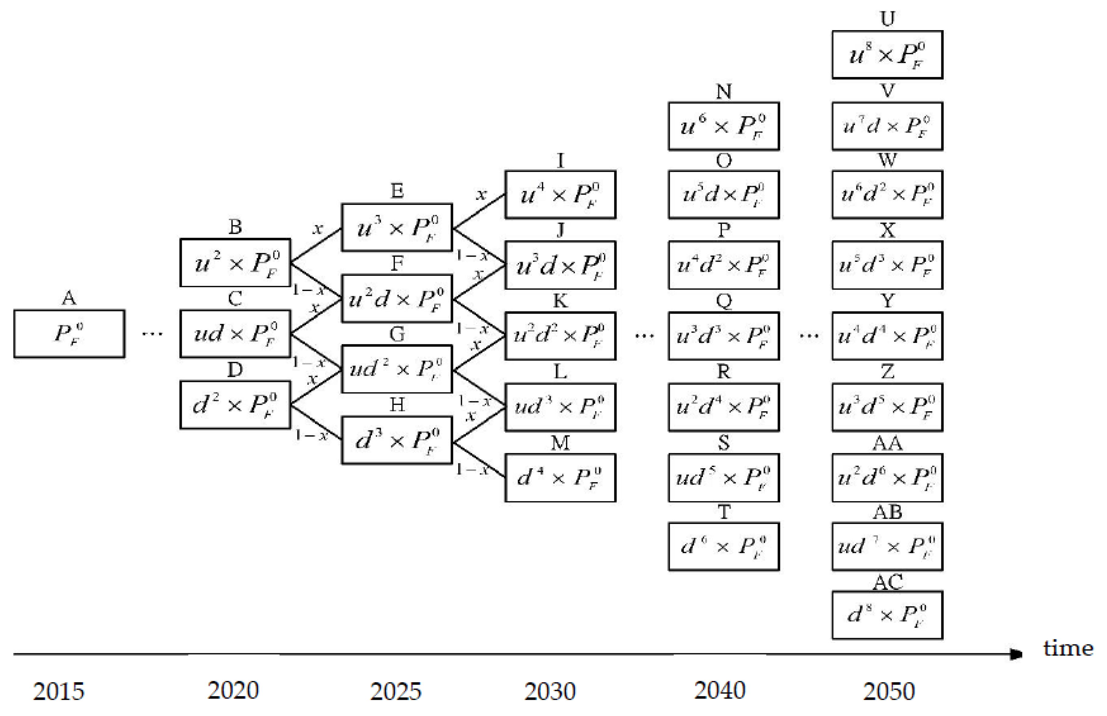
2.3. The Unit Power Generation Cost Prediction under Uncertainty

This research refers to the risk neutral probability method of real option analysis (ROA) (Copeland and Antikavro (2001) [22], which will incorporate the cost randomness of various power generation technologies, then estimate the pathway of unit power generation costs by 2050.

2.3.1. The Average Growth Rate of Unit Power Generation Cost

This applies the ROA method to estimate the growth rate and decline rate of unit power generation cost of various power generation technologies as follows:

$$u=e^{gt}$$

(11)

$$d=1/u,$$

(12)

This study collected the unit power generation cost (US$/kWh) of various power generation technologies of the Taiwan Power Company (2016) [23] (see

Table 1. Parameters value of various power generation technologies.

	Technology	Pumped-Storage Hydroelectricity	Coal-Fired Power	Oil-Fired Power	Gas-Fired Power	Nuclear Power	Renewable Energy Resources
Parameter
Unit cost of power generation ($P_0^F$) (US$/kWh)		0.14	0.05	0.15	0.09	0.04	0.07
Capacity factor (${\varpi }_i$) (%)		16.59	89.23	40.48	70.00	80.94	35.26
αi		0.5	0.5	0.5	0.5	0.5	0.5
Annual growth rate of unit power generation cost ($g$) (%)		6.77	3.40	3.50	1.18	10.92	5.02
Risk-free rate ($r_f$) (%)		1.18	1.18	1.18	1.18	1.18	1.18
Increasing rate of unit cost (u) (%)		1.403	1.185	1.191	1.061	1.726	1.285
Decline rate of unit rate (d) (%)		0.713	0.844	0.839	0.942	0.579	0.778
Allocation ratio of increasing rate (x) (%)		43.33	49.21	48.98	58.47	37.71	46.08
Allocation ratio of decline rate (1 − x) (%)		56.67	50.79	51.02	41.53	62.29	53.92

Source: this research.

). The unit cost of oil-fired power generation reached 0.15 US$/kWh, which was the most expensive, but the unit cost of nuclear power generation was only 0.04 US$/kWh, which was the cheapest. Further, the study estimates the average annual unit power generation cost growth rate ($g$) of various power generation technologies from 2005 to 2015 (see Table 1). This show that nuclear has the highest average annual growth rate (10.92%) of unit power generation costs, but gas has the lowest average annual growth rate (1.18%) of unit power generation costs.

2.3.2. The Change Rate of Unit Power Generation Cost Estimation

$$x=\frac{(1+r_f)-d}{u-d}$$

(13)

where $u$ is the increasing rate of unit power generation cost, $d$ is the decline rate of unit power generation cost, $g$ is the annual average growth rate of unit generation cost and $t$ is the interval of each stage (let $t$ = 5). The $u$ and $d$ values of various power generation technologies are summarized as shown in Table 1. x and 1 − x are the ascending path allocation ratio and the descending path allocation ratio respectively (refer to Copeland and Antikavro (2001) [22]). This study uses the risk-neutral probability method, such as Equations (11) and (12), to calculate the ascending (x) and descending (1 − x) path allocation rates. Substituting the risk-free interest rate ($r_f=1.18\%$) (This research refers to the 10-year central government bond yield rate of the Central Bank of Taiwan in 2015 as 1.18%), the estimated value of unit cost growth rate and decline rate into Equations (12) and (13), we can get the distribution ratios of various annual growth and decline rate of various unit cost of power generation technology. The results are obtained of various parameter, see Table 1.

2.3.3. Capacity Factor and Technology Factor

The study collected the capacity factor (${\varpi }_i$) of various power generation technology form the Taiwan Power Company (2016) [22], as shown in Table 1. This indicates that nuclear and coal-fire have the highest capacity factors of 89.9% and 88.87%, respectively. This reflects the characteristics of the base load of this two power generation technologies. The capacity factors of pumped-storage and oil-fired are the lowest, 13.5% and 18.6%, respectively.

To simplify the analysis, the research assumes technology factor ($\alpha$) as shown in Table 1. Then, a form of long-term random unit cost power generation trajectory is shown in Figure 1.

3. Results and Discussion

3.1. Optimal Power Generation Portfolio Estimation

3.1.1. Long-Term Unit Cost of Power Generation Estimation

Taking the unit coal-fired power generation cost as an example, the growth rate of coal cost is 1.185% and the decline rate is 0.844%. Then, the unit cost at different stages can be calculated. See the calculation method in Figure 1. It could be obtained that the highest unit cost of coal-fired power generation by 2050 can rise to 0.086 US$/kWh, and the lowest can be reduced to 0.025 US$/kWh (see

Table 2. Estimation of unit power generation cost in high, medium and low scenarios. Unit: US$/kWh.

	Fuel	Pumped-Storage Hydroelectricity	Coal-Fired Power	Oil-Fired Power	Gas Power	Nuclear Power	Renewable Energy Resources
Scenarios
2020	high	0.191	0.055	0.173	0.099	0.066	0.095
	medium	0.144	0.047	0.147	0.093	0.044	0.076
	low	0.097	0.039	0.122	0.088	0.022	0.058
2025	high	0.202	0.056	0.175	0.099	0.076	0.098
	medium	0.158	0.048	0.151	0.094	0.055	0.080
	low	0.069	0.033	0.102	0.083	0.013	0.045
2030	high	0.221	0.057	0.180	0.099	0.095	0.103
	medium	0.178	0.050	0.156	0.094	0.073	0.086
	low	0.073	0.033	0.104	0.083	0.015	0.046
2040	high	0.350	0.070	0.222	0.106	0.218	0.142
	medium	0.246	0.054	0.172	0.095	0.147	0.104
	low	0.057	0.029	0.089	0.079	0.011	0.038
	high	0.571	0.086	0.276	0.113	0.524	0.199
2050	medium	0.368	0.062	0.196	0.097	0.330	0.133
	low	0.046	0.025	0.078	0.074	0.008	0.020

Source: This research.

). The calculation of other power generation unit costs is the same way.

The article divides the random fuel cost of future power generation technologies into high, medium, and low case for analysis. The high case is the average cost of each year greater than or equal to the median value (including the median value), and the medium case is the average of all random costs. The low case is the average cost of each year less than or equal to the median value (including the median value). Taking the unit cost of coal-fired random power generation as an example, there are two cost values in 2020. The high cost is 0.173 US$/kWh and the low cost is 0.122 US$/kWh. The average cost is 0.147 US$/kWh (see Table 2). The calculation of other power generation unit costs is performed the same way.

3.1.2. CO₂ Emission Target by 2050

The Taiwanese government has set up national greenhouse gas emissions targets to respond to climate change, namely reducing greenhouse gas emissions to 257 MtCO₂e by 2020, 205.6 MtCO₂e by 2030, and 128.5 MtCO₂e by 2050. According to this emissions trajectory, the estimation of CO₂ emissions target is 179.7 MtCO₂e by 2040. In addition, the CO₂ emissions share of the power generation sector account for 41.4% of total domestic CO₂ emissions. Then, we can calculate the CO₂ emissions targets by the power generation sector: 106.4 MtCO₂e by 2020, 85.1 MtCO₂e by 2030, 73.4 MtCO₂e by 2040, and 53.2 MtCO₂e by 2050 (see

Table 3. The trajectory of power generation, CO₂ emissions and reasonable risk value.

	Target	Power Generation (GWh/Year)	CO2 Emissions (MtCO2e)	Risk Value
Year
2020		249,290	106.4	0.1118
2025		234,748	95.8	0.2537
2030		218,151	85.1	0.2537
2040		200,715	73.4	0.2537
2050		165,534	53.2	0.2537

Source: This research.

).

3.1.3. Reasonable Risk Value by 2050

Reasonable risk value refers to the risk value of the power generation technology portfolio that could maintain sufficient economic dispatch of the power generation system (Awerbuch and Spencer, 2007; Huang and Lee, 2019). The economic dispatch of the power generation system portfolio should get better. This article sets the risk value (0.2537) in 2015, which is the default value of the reasonable risk value. This means that the risk value of the future power generation mixed must be less than 0.257. We calculate the long-term trajectory of the risk value of the power generation technology portfolio as shown in Table 3.

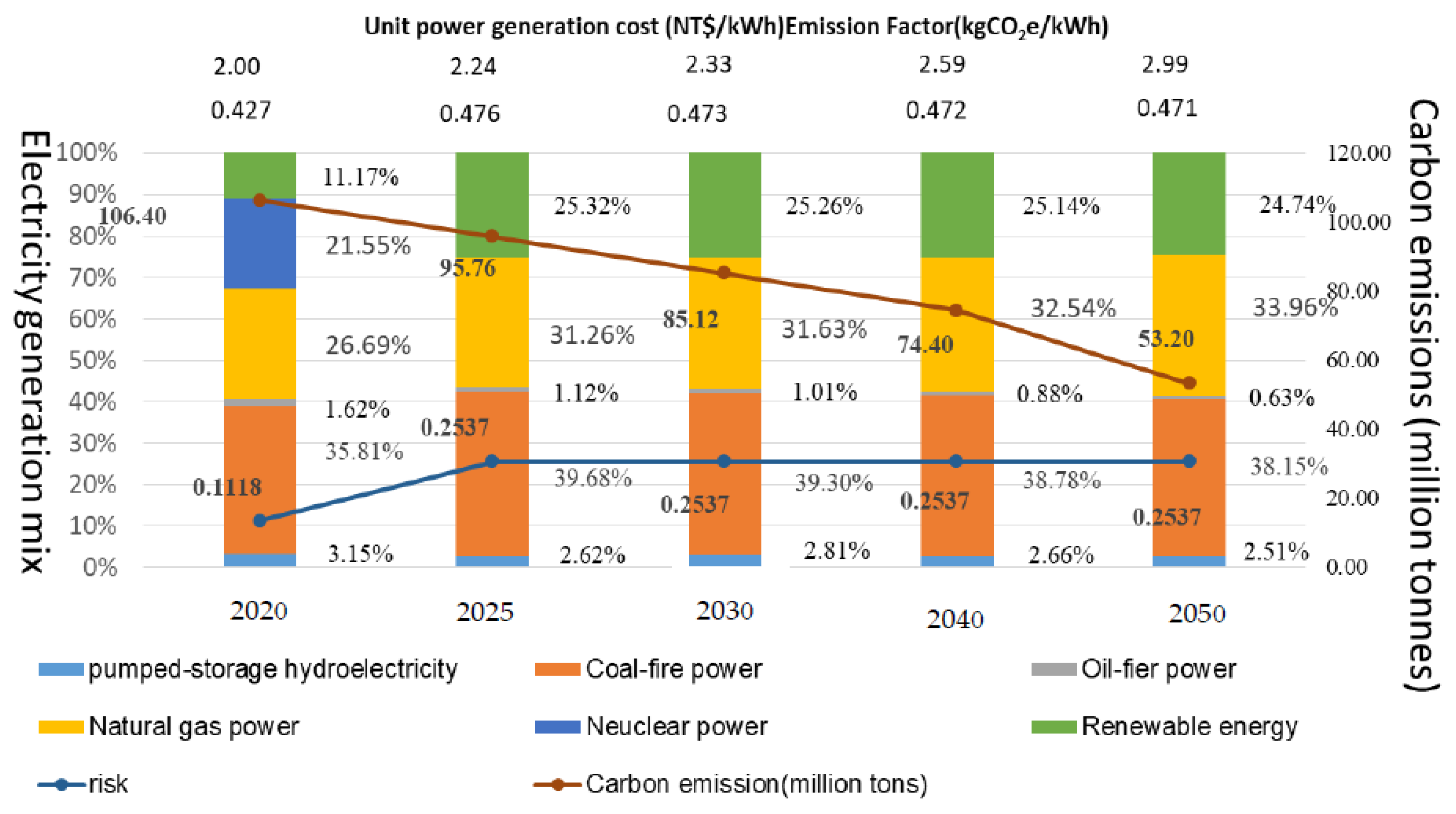
3.1.4. Optimal Power Generation by 2050

The optimal power generation trajectory refers to the feasible power generation in each period that simultaneously meets the CO2 emission limitation and reasonable risk value. Then, we could calculate the pathway of power generation as: 249,290 GWh (2020), 234,748 GWh (2025) 218,151 GWh (2030), 200,715 GWh (2040), and 165,534 GWh (2050), respectively (see Table 3).

3.1.5. Optimal Power Generation Mixed

The Taiwanese government has set a goal for a nuclear-free country by 2025. This study assumes that, after 2025, the nuclear power generation ratio will decline to zero. Based on this, the research takes a medium-scenario fuel cost as an example (see Table 2), subject to the conditions and restrictions of each period in Table 3. Putting the relevant parameters into Equation (10)—as data on the marginal cost of carbon reduction in the power generation sector is not easy to obtain, in order to simplify the analysis, the cost of abatement ($P_{A}e$) is not calculated—we obtain power generation mixed by 2050, as shown in Figure 2. Figure 2 was showed the optimal power generation technology mixed during the period 2020–2050 in Taiwan. It indicates that the unit cost of power generation will increase gradually from 2020 to 2050, from 1.81 NT$/kWh to 2.77 NT$/kWh. The share of renewable energy and gas power will increase gradually, as the former will increase from 16.11% (2020) to 52.67% (2050) and the latter will increase from 16.42% (2020) to 17.82% (2050). In contrast, the share of coal-fired power will decrease from 33.43% (2020) to 25.64% (2050).

Renewable energy is carbon-free and complementary to fossil fuels. It has the advantage of reducing risk value, but the disadvantage of high cost. Therefore, it can meet the CO₂ target and reasonable risk value at the same time. Under the condition of reasonable risk value, the ratio of renewable energy power generation should be maintained at about 25%. Especially after being nuclear-free by 2025, the ratio of renewable energy is the key power generation technology to support the national low-carbon target and the low risk value of the power generation system. Gas-fired power generation has low-carbon advantage, but high cost and substitution with other fossil fuels, having the disadvantage of increasing the value of risk. Therefore, after being nuclear-free by 2025, although the share of power generation will be greatly increased by 31% (additional low-carbon requirements), it can only be maintained at a ratio of slightly higher than 30%. Coal-fired power generation has low cost, but high CO₂ emissions and its substitution with other fossil fuels, this disadvantage for improving risk value. Therefore, after being nuclear-free by 2025, although the share of power generation will be slightly increased by 39% (to supplement the power supply security and low-cost requirements), as the proportion of renewable energy and gas power generation increases, coal-fired power generation will suffer from high CO₂ emissions restrictions, as the mixed power generation will drop slightly to 38%.

3.2. Optimal Electricity Saving Planning

This article aims to limit the country’s electricity demand through long-term optimal power generation. This method is feasible and necessary under the development of net zero emissions, because hydrogen energy and decentralized grids and other energy saving innovation are under schedule in the agenda and could be used to greatly reduce electricity demand.

In the following sections, we will use the STIRPAT model with PLS regression to predict the electricity demand baseline (or business as usual), then provide the optimal electricity saving trajectory by 2050.

3.2.1. STIRPAT Regression Model

Dieta and Rosa (1997) [24] proposed the STIRPAT (Stochastic Impacts by Regression on Population, Affluence, and Technology) model, it has been widely used in forecasting for various economic activities (York et al., 2003) [25]. This study chooses two key variables, GDP per capita and energy intensity, affecting power consumption in the ATIRPAT model. GDP per capita captures both the population and affluence as two variables, and energy intensity describes energy technology. The STIRPAT model can be expressed as Equation (14):

$$\ln E_t=a_0+{\alpha }_1\ln GDP{P}_t+{\alpha }_2\ln EGD{P}_t+\epsilon$$

(14)

where $E_t$ is the electricity demand in year t; $GDP{P}_t$ is the GDP per capita in year t; $EGD{P}_t$ is the energy intensity in year t; $a_0$ is constant term; ${\alpha }_1$ and ${\alpha }_2$ are the regression coefficients of variables of GDP per capita and energy intensity respectively; ${\epsilon }_t$ is the error term.

3.2.2. Data Collection and Settings

This study uses the “Energy Statistics Manual” published by the Bureau of Energy [26] in 2015 to collect data on electricity demand and energy intensity. It also uses the statistics information network of the Republic of China to collect data on per capita GDP and energy intensity. The year range for the completeness of the data is from 1998 to 2015.

This study aims to predict the medium and long-term electricity demand in Taiwan. It is planned to set the forecast value for each independent variable, as shown in

Table 4. Data sources and setting of variables.

Variable	Data Source	Setting of Prediction Value
GDP per capita	National Statistics, Taiwan.	Estimated using the average annual growth rate of 2.92% as calculated from the data of GDP per capital in the past 10 years.
Energy intensity	Bureau of Energy (2015), “Energy Statistics Handbook” [26]	Estimated using the average annual decline rate of 1.45% from 1998 to 2015.
Electricity demand amount	Bureau of Energy (2015), “Energy Statistics Handbook” [26]	Projected by substituting the independent variables into the model as established using the regression results.

Source: This research.

. Per capita GDP is estimated based on data from the past 10 years (2006 to 2015) and an average annual growth rate of 2.92% is calculated. The energy intensity is estimated based on the data from 1998 to 2015, and the annual average decline rate is calculated to be 1.45%, while electricity demand is estimated by using the model established by the regression results to bring in the predicted values of the respective variables for medium and long-term estimation.

Based on this, this study estimates the predicted values of each variable in 2020, 2025, 2030, 2040, and 2050, as shown in

Table 5. Predicted value of selected variable.

	Year	2020	2025	2030	2040	2050
Variable
GDP per capita (NT$/population)		824,868	952,581	1,100,068	1,467,084	1,956,547
Energy intensity (Liter oil equivalent/NT$1000)		6.83	6.35	5.91	5.11	4.42

Source: This research.

.

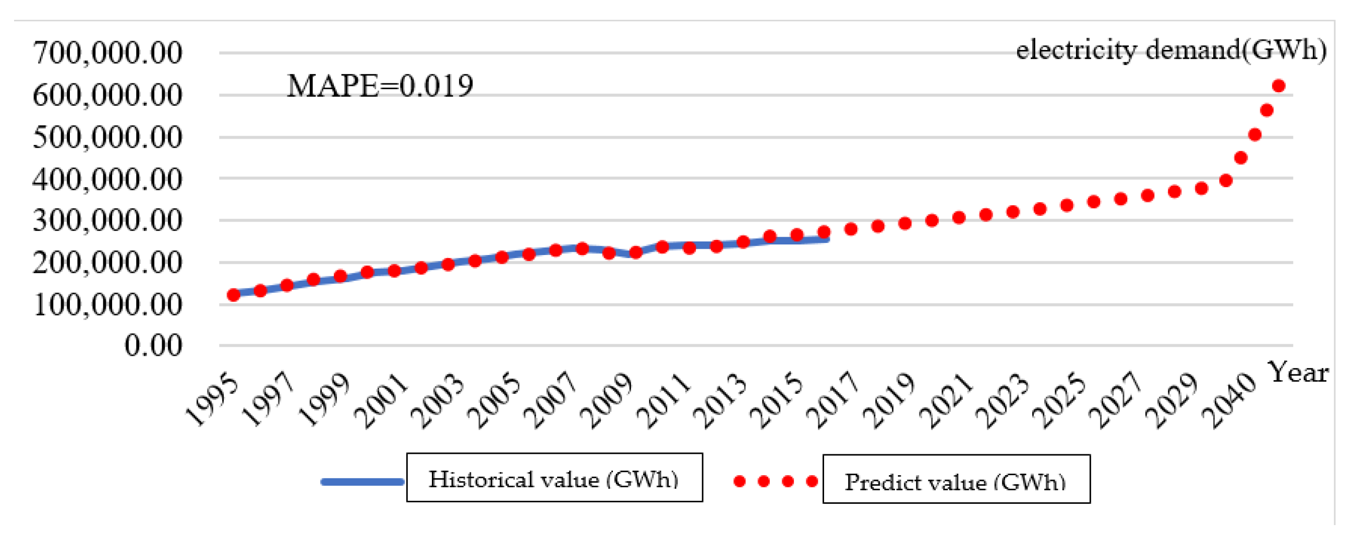
3.2.3. Prediction of the Electricity Demand

The correlation of the independent variables of the STIRPAT model is shown in

Table 6. The results of Correlation Coefficient of Regression Variables.

	$\mathit{G}\mathit{D}\mathit{P}\mathit{P}$	$\mathit{E}\mathit{G}\mathit{D}\mathit{P}$
$GDPP$	1.000	0.784
$EGDP$	0.784	1.000

Source: This research.

, where the variables have a high linear correlation. Therefore, this study uses the partial least squares regression (PLS-R) method for regression analysis.

The results of PLS regression as shown in Equation (15), which present that all variables are 1% significant (See

Table 7. The results of regression.

Variables	Coefficient	t Value	p Value	${\mathit{R}}^2$
Constant	−7.421 ***	−9.116	0.00	0.988
GDPP	1.379 ***	28.450	0.00
EGDP	0.673 ***	6.998	0.00

Note: *** present 1% significant. Source: This research.

). This study further calculated the mean absolute percentage error (MAPE) based on the actual electricity demand from 1998 to 2015. As shown in Figure 3, the MAPE value is very small (0.019), indicating that the regression equation (Equation (15)) has a high accuracy for the electricity demand prediction.

$$\ln E_t=-7.412+1.379\ln GDP{P}_t+0.673\ln EGD{P}_t$$

(15)

3.2.4. The Trajectory of Electricity Saving by 2050

Under the regression equation of Equation (15), the prediction of electricity demand from 2020 to 2050 is shown in

Table 8. The trajectory of electricity saving by 2050.

	2020	2025	2030	2040	2050
Electricity supply (GWh)	249,290	234,748	218,151	200,715	165,534
Electricity demand (GWh))	302,002	340,681	384,314	489,061	622,358
Electricity Saving (GWh)	52,712	105,933	166,163	288,346	456,824
Electricity Saving rate (%)	17.5	31.1	43.2	59.0	73.4

Source: This research.

. It shows the electricity demand going up along with time, from 302,002 GWh in 2020 to 622,358 GWh in 2050. Since electricity saving is the priority strategy to achieve greenhouse gas emissions targets and maintain power supply security, this study can calculate the power saving requirements for each period in the future, such as 52,712 GWh/year (17.5% accumulative saving rate) (2020), 105,933 GWh/year (31.1% accumulative saving rate) (2025), 166,163 GWh/year (43.2% accumulative saving rate) (2030), 288,346 GWh/year (59.0% accumulative saving rate), and 288,346 GWh/year (73.4% accumulative saving rate) (2050). This result can provide a reference for the Taiwan government to plan its active electricity saving target by 2050.

4. Conclusions

This research considers long-term power generation portfolio planning that simultaneously meets the requirements for power generation security, greenhouse gas reduction targets, and reasonable risk value. While the model developed is new, it provides significant policy implications. In terms of research methods, this research uses an optimal control model to establish a theoretical basis for calculating the long-term dynamic path of various the power generation mixed, which is innovative in terms of methodology. Meanwhile, this research uses the theory of real options to capture the randomness of long-term unit power generation costs of various power generation technologies. This study points out that the target power generation mix set by the Taiwanese government for 2025 is not consistent with a low-carbon transition. Indeed, the share of renewable energy should be increased to 25% to reflect its complementarity with other power generation technologies for the economic dispatching requirements of a power system. Being environmentally friendly and socially acceptable, the ratio should be maintained at about 25% to maintain the reliability of the power generation system (low risk value). The coal ratio should be adjusted to reflect affordability and economic efficiency, and in the medium and long term, it should be controlled below 40% to match the requirement of affordability. The share of natural gas should be reduced for affordability, and in the medium and long term, it should be maintained at about 30% to reflect the environmental friendliness of low-carbon energy. Furthermore, we apply the STIRPAT model with PLS regression to predict the electricity demand baseline (or business as usual), providing a feasible electricity saving trajectory by 2050.

This article tries to adopt a viewpoint of sustainable development, which evaluates the country’s long-term power mix. Therefore, the research approach is different from the traditional view. This article aims to limit the country’s electricity demand through the principle of “supply dictates demand”. The result is feasible under the development of low carbon technology, like hydrogen energy and decentralized grids, as well as other developing rapidly innovations in climate finance which could be used to greatly reduce electricity demand.

References

1. Seto, K.C.; Davis, S.J.; Mitchell, R.B.; Stokes, E.C.; Unruh, G.; Ürge-Vorsatz, D. Carbon lock-In: Types, causes, and policy implications. Annu. Rev. Environ. Resour. 2016, 41, 425–452. [Google Scholar] [CrossRef] [Green Version]
2. Intergovernmental Panel on Climate Change. Global Warming of 1.5 °C; IPCC Special Report 2018; IPCC: Geneva, Switzerland, 2018; Available online: https://www.ipcc.ch/sr15/ (accessed on 23 October 2017).
3. Awerbuch, S.; Spencer, Y. Efficient electricity generating portfolios for Europe: Maximizing energy security and climate change mitigation. EIB Pap. 2007, 12, 8–37. [Google Scholar]
4. DeLlano-Paz, F.; Fernandez, P.M.; Soares, I. Addressing 2030 EU policy framework for energy and climate: Cost, risk and energy security issues. Energy 2016, 115, 1347–1360. [Google Scholar] [CrossRef]
5. DeLlano-Paz, F.; Fernandez, P.M.; Soares, I. The effects of different CCS technological scenarios on EU low-carbon generation mix. Environ. Dev. Sustain. 2016, 18, 1477–1500. [Google Scholar] [CrossRef]
6. Min, D.; Chung, J. Evaluation of the long-term power generation mix: The case study of South Korea’s energy policy. Energy Policy 2013, 62, 1544–1552. [Google Scholar] [CrossRef]
7. Zhang, S.; Zhao, T.; Xie, B.C. What is the optimal power generation mix of China? An empirical analysis using portfolio theory. Appl. Energy 2018, 229, 522–536. [Google Scholar] [CrossRef]
8. Wu, J.H.; Huang, Y.H. Electricity portfolio planning model incorporating renewable energy characteristics. Appl. Energy 2014, 119, 278–287. [Google Scholar] [CrossRef]
9. Li, S.; Mu, H.; Guiand, S.; Li, M. Scenario analysis for optimal allocation of China’s electricity production system. Sustain. Cities Soc. 2014, 10, 241–244. [Google Scholar] [CrossRef]
10. Chen, F.F.; Chou, S.C.; Lu, T.K. Scenario analysis of the new energy policy for Taiwan’s electricity Sector until 2025. Energy Policy 2013, 61, 162–171. [Google Scholar] [CrossRef]
11. Tsain, M.S.; Chang, S.L. Taiwan’s 2050 low carbon development roadmap: An evaluation with the MARKAL model. Renew. Sustain. Energy Rev. 2015, 49, 178–191. [Google Scholar]
12. Lee, C.M.; Rosalez, E.R. Economic growth, carbon abatement technology and decoupling strategy—The case of Taiwan. Aerosol Air Qual. Res. 2017, 17, 1549–1557. [Google Scholar] [CrossRef] [Green Version]
13. Blancoa, H.; Nijsb, W.; Rufc, J.; Faaija, A. Potential of power-to-methane in the EU energy transition to a low carbon system using cost optimization. Appl. Energy 2018, 232, 323–340. [Google Scholar] [CrossRef]
14. Ryu, H.; Dorjragchaa, S.; Kim, Y.; Kim, K. Electricity-generation mix considering energy security and carbon emission mitigation: Case of Korea and Mongolia. Energy 2014, 64, 1071–1079. [Google Scholar] [CrossRef]
15. Portugal-Pereira, J.; Esteban, M. Implications of paradigm shift in Japan’s electricity security of supply: A multi-dimensional indicator assessment. Appl. Energy 2014, 123, 424–434. [Google Scholar] [CrossRef]
16. Troldborg, M.; Heslop, S.; Hough, R. Assessing the sustainability of renewable energy technologies using multi-criteria analysis: Suitability of approach for national-scale assessments and associated uncertainties. Renew. Sustain. Energy Rev. 2014, 39, 1173–1184. [Google Scholar] [CrossRef]
17. Kumar, A.; Sahb, B.; Singhc, A.R.; Denga, Y.; Hea, X.; Kumarb, P.; Bansald, R.C. A review of multi criteria decision making (MCDM) towards sustainable renewable energy development. Renew. Sustain. Energy Rev. 2017, 69, 596–609. [Google Scholar] [CrossRef]
18. Choi, D.H.; Ahn, Y.H.; Choi, D.G. Multi-criteria decision analysis of electricity sector transition policy in Korea. Energy Strategy Rev. 2020, 29, 100485. [Google Scholar] [CrossRef]
19. Huang, Y.H.; Lee, C.M. Designing an optimal water supply portfolio for Taiwan under the impact of climate change: Case study of the Penghu area. J. Hydrol. 2019, 573, 235–245. [Google Scholar] [CrossRef]
20. Su, K.; Lee, C.M. When will China achieve its carbon emission peak? A scenario analysis based on optimal control and the STIRPAT model. Ecol. Indic. 2020, 112, 106138. [Google Scholar] [CrossRef]
21. Pan, B.; Zhang, Y. Impact of affluence, nuclear and alternative energy on US carbon emissions from 1960 to 2014. Energy Strategy Rev. 2020, 32, 100581. [Google Scholar] [CrossRef]
22. Copeland, T.; Antikarov, V. Real Options: A Practitioner’s Guide; University of Michigan: Texere, NY, USA, 2001; Available online: https://books.google.com.tw/books/about/Real_Options.html?id=fnhPAAAAMAAJ&redir_esc=y (accessed on 8 November 2007).
23. Taiwan Power Company. Long-Term Financial Planning and Capital Expenditure Control Project Group; Accounting Office Newsletter of Taiwan Power Company: Taipei city, Taiwan, 2016. [Google Scholar]
24. Dietz, T.; Rosa, E.A. Rethinking the environmental impacts of population, affluence and technology. Hum. Ecol. Rev. 1994, 1, 277–300. [Google Scholar]
25. York, R.; Rosa, E.A.; Diet, Z.T. STIRPAT, IPAT and ImPACT: Analytic tools for unpacking the driving forces of environmental impacts. Ecol. Econ. 2003, 46, 351–365. [Google Scholar] [CrossRef]
26. Bureau of Energy Bureau of Energy. Energy Statistics Handbook 2015; Ministry of Economic Affairs: Taipei city, Taiwan, 2015.
Figure 1. The long-term unit cost of power generation estimation. (US$/KWh). Source: This research.
Energies 14 04402 g001
Figure 2. The optimal power generation technology mixed (2020–2050) in Taiwan. Source: This research.
Energies 14 04402 g002
Figure 3. The MAPE (from 1998–2015) and electricity demand predict by 2050. Source: This research.
Energies 14 04402 g003