Abstract
Wind turbines are often placed in complex terrains, where benefits from orography-related speed up can be capitalized. However, accurately modeling the wind resource over the extended areas covered by a typical wind farm is still challenging over a flat terrain, and over a complex terrain, the challenge can be even be greater. Here, a novel approach for wind resource modeling is proposed, where a linearized flow model is combined with a machine learning approach based on the k-nearest neighbor (k-NN) method. Model predictors include combinations of distance, vertical shear exponent, a measure of the terrain complexity and speedup. The method was tested by performing cross-validations on a complex site using the measurements of five tall meteorological towers. All versions of the k-NN approach yield significant improvements over the predictions obtained using the linearized model alone; they also outperform the predictions of non-linear flow models. The new method improves the capabilities of current wind resource modeling approaches, and it is easily implemented.
1. Introduction
Wind and solar photovoltaic power plants are now the cheapest options for electricity generation in most parts of the world [], paving the way for the extensive decarbonization [,,] of the power sector and the economy. However, in the case of wind energy, the accurate assessment of the wind resource at a prospective wind farm site continues to be key to successful development and competitive pricing. While traditional modeling approaches [,] for wind project development [] are often sufficiently accurate in flat or mildly rolling landscapes, wind power predictions in complex terrain are considerably more challenging [,,,,]. A 5% mean error in predicted wind speed can be the threshold for the approval or rejection of a wind project. Although traditional modeling approaches based on linearized flow solvers are nowadays often complemented with Reynolds-averaged Navier–Stokes (RANS) flow models and sometimes even large-eddy simulations (LES), the benefit is not always clear. Well-tuned linearized flow models, complemented by expert knowledge, may often yield similar or better results compared to advanced computational fluid dynamics (CFD) models.
In an attempt to evaluate and compare the performance of numerical wind flow models, different validation studies have been reported in the literature. Flow modeling approaches include assessments using wind industry-standard linearized flow models such as the one included in the Wind Atlas Analysis and Application Program (WAsP) [], and more complex CFD approaches, e.g., RANS and LES. Beaucage et al. [] performed a validation study over different terrain features, where the linearized flow model in WAsP and the Meteodyn CFD model were compared. In contrast to what is normally assumed, the results of WAsP were similar or better than those of the CFD model, with an overall root mean squared error (RMSE) of 0.62 m/s (corresponding to an 8.0% error) for WAsP and 0.76 m/s (9.4%) for Meteodyn. Another comparative analysis was performed between the linearized WAsP model and the RANS-model also available within the WAsP suite (WAsP CFD) at a complex site in Brazil []. In this study, it was pointed out that the WAsP CFD model did not present a clear advantage over the linearized version. The authors conjectured that thermal effects not considered by either model highly contributed to the uncertainty of both results. Other studies have suggested the capacity of CFD models to outperform linear models [,,]; Hristov et al. [] suggested improvements of about 8% when predicting the annual energy production (AEP).
More recently, statistical learning methods have made their appearance in wind resource assessment. Such methods have the potential for taking advantage of a larger amount of input data than conventional approaches. In such data-based methods, the learning process commonly relies on terrain and meteorological features to estimate the target variable. This provides greater flexibility for considering micro-climatic effects that are generally not accounted for by flow models. Examples of machine learning methods include ensembles of regression trees [], support vector regression (SVR) [] and neural networks (NN) [].
The combination of physics-based and data-based methods may be a natural solution to the problem of accurate wind resource estimations in a complex terrain. Such hybrid approaches take advantage of each method’s strengths to increase robustness and predictive performance. However, for wind resource assessment, these methods are less popular. According to a literature review, only Tang et al. [] appear to have used a method that combines flow (CFD) simulations with a data-driven technique for assimilating multiple on-site measurements in complex terrain, in addition to a more traditional inverse-distance weighting (IDW) method [].
Here, we address the continuing challenges of accurate wind resource estimation in complex terrains by designing a method which taps into the capabilities of modern wind resource modeling suites such as WAsP or WindSim, but simultaneously provides the capability of accounting for micro-climatic effects, which are generally not properly addressed in flow models. The proposed new method is based on a conceptually simple machine learning approach, the k-nearest neighbors (k-NN) method (see, e.g., []). To the best of our knowledge, this approach has not been used before. The basic idea was to take advantage of the similarity between different locations at a prospective wind farm site in terms of a set of classifiers or features (Section 2.1). Ideally, it should be possible to determine such features with the terrain information alone (elevation and roughness) and possibly wind resource information from one reference location, very much like in conventional flow models. It will be argued below that all feature parameters required for this work can actually be determined with flow models such as WAsP or WindSim alone, although an improved prediction can be obtained in the case of power density estimates if the wind rose at one reference location is known. The new k-NN method can then be used in complete analogy to a conventional flow model to predict the wind resource at an arbitrary location for the purpose of turbine yield calculation or wind mapping. It should be noted that while the new method essentially uses the same input information as a conventional flow model, it provides larger flexibility, since it is not restricted by the deterministic relationships between a target and a reference location, which necessarily only consider the properties of the fluid model but not the micro-climate.
In order to build a reference case against which the new method can be compared, flow simulations based on both the linearized model within the WAsP suite (Section 2.6) and the RANS-CFD model (WindSim) (Section 2.7) were conducted first and the results were analyzed by cross-validation. The setup of both models was explored in a detailed manner, ensuring that the models were optimally configured and not artificially underperforming. This included the fine-tuning for atmospheric stability (in the case of WAsP), the use of both standard and high-resolution roughness maps, the exploration of a detailed forest model (in the case of WindSim), and the study of two different turbulence closure models (in the case of WindSim).
A number of different implementations were studied for the k-NN approach (Section 2.4). The basic approach consists of directly using the observed wind speed or power density at the available met tower locations, with the exception of the target location used for validation in each turn. Alternatively, the local wind climates can be first transferred to the target location, and the k-NN can then be applied to the transferred climates; this is what we call the hybrid approach below. Given that the hybrid method is a statistically independent implementation, the linear combination of both methods, i.e., an ensemble, bears the potential of providing more accurate predictions and was implemented as well.
2. Methods and Data
2.1. The k-NN Method Applied to Wind Resource Modeling: The General Concept
The general idea of the k-NN approach is to determine similarity between different locations, using a certain number of features as variables in a generalized coordinate space. Each site can then be represented as a point in this -dimensional space, and its distance from any other site can be determined by an appropriate norm. Here, the L2-norm was used throughout, prior to the standardization of each feature variable x through . Feature candidates include strictly terrain-related variables, such as the terrain complexity parameter RIX [], speedup and (geometric) distance between sites; variables related to local atmospheric conditions, such as temperature and turbulence intensity; and mixed variables such as the vertical wind shear, which depend on both terrain-dependent flow and atmospheric stability.
The key assumption of the k-NN method is that the variable of interest, e.g., the wind speed at time step , can be predicted from the values of its k nearest neighbors in the -dimensional feature space, either by a simple or a weighted average:
where is the target site and is the set of nearest neighbors identified by the algorithm. The weights were taken either as constant (uniform weighting) or as (inverse distance weighting, IDW), where is the distance between features (=. It should be noted that the number k of nearest neighbors can be dynamically determined at each time step by the algorithm, allowing to account for time-dependent features.
The k-NN procedure is illustrated in Figure 1 for the case of two features, which in this case are the RIX number and the speedup. The differences in RIX between the predictor and the predicted site (delta-RIX) can be used to correct results obtained with the linearized flow model in WAsP for complex terrain analysis []. Here, RIX is used as one of the potential features determining similarity. In Figure 1, the target site is shown is a diamond-shaped location in the RIX-speedup plane, together with a number of potential predictor sites. Note that both features may be taken as constant or time dependent; in the more general case of time-dependent features, Figure 1 shows a snapshot of a set of locations at a given time step . The methodology can also be extended to include the time as an additional feature.
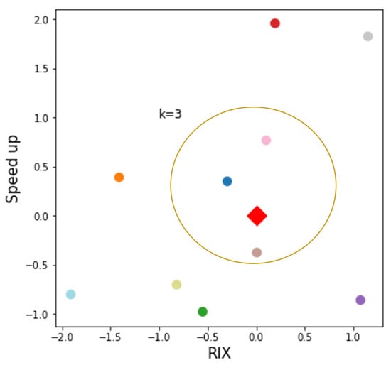
Figure 1.
Illustration of the k-NN approach, for the case of the features’ speedup and RIX. Red diamond: target site. The circles groups the k = 3 nearest neighbors out of 10 possible predictors.
2.2. Hyperparameter Estimation in k-NN Models
In a k-NN regression, the number of nearest neighbors in feature space k is a hyperparameter that determines the accuracy of the model. The other hyperparameter used in this work is the type of weighting (uniform or inverse-distance weighting); see Equation (1). Both hyperparameters are evaluated systematically in a process called parameter tuning, which determines the optimal value of k so that prediction errors are minimized. The standard methodology is based on splitting the data set into a training and a testing set, in such a way that the training set allows to estimate the optimal value (usually by cross-validation to avoid over-fitting). Then, the selected value is evaluated on the testing set (unseen data) to obtain an unbiased estimation of the model’s performance. In the present work, this approach was used for reference purposes (see below), however, the main contribution of this work to the k-NN methodology is the estimation of the optimal hyperparameters without the target location, while still using the full observational period, thereby avoiding seasonality biases; a detailed description can be found in Section 2.4. The two conceptually different approaches used in the work for hyperparameter estimation can then be described as follows:
- In the first approach, the complete annual set of wind measurements was used to obtain the minimizing the prediction errors for each site. In a first step (termed method kNN0 in Section 2.4), data from all locations, including the target site, were used for that purpose. This step provides a fit to the data, not a prediction. It does, however, allow creating prior knowledge of the best hyperparameters possible for the reference sites. An estimation of the optimal hyperparameters without using data from the target site, required for wind resource estimation at a location without measured data, is then conducted in a separate step, as described in Section 2.2.1.
- The second approach consists of the implementation of a nested cross-validation method, similar to the standard procedure of splitting the data set into a training and evaluation set. As opposed to the standard procedure, however, biases are avoided by using training periods of variable lengths, while maintaining validation and testing periods at constant lengths; as can be seen in Section 2.2.2.
2.2.1. Hyperparameter Estimation with the Full Data Set
The parameter estimation for the full observational period is based on the following four algorithms. Algorithm 1 estimates the wind speed at each time step i using multiple combinations of features and a maximum of k neighbors. The uniformly weighted k-NN average and the inverse-distance weighted k-NN prediction were used to estimate the wind speed. The mean percentage error MPE was used as the main error metric.
Algorithm 2 was used to determine the best hyperparameter k and its associated regression type c, either uniform or inverse-distance weighted. Those best ks were selected for each site and for each set of features based on their MPE values. A ranking of the best set of features for the study site was determined by cardinality (i.e., the number of features in a set) based on the average of the MPE of all sites. Here, the four highest-ranking sets of features (i.e., the four best indicators of similarity) are reported in all cases.
| Algorithm 1k-NN regression with subset and number of neighbors selection |
|
| Algorithm 2 Selection of the optimal k and best predictors for cardinality 2 to |
|
As mentioned previously, the optimal hyperparameters ( and ) determined by Algorithm 2 (also referred to as method kNN0, as can be seen in Section 2.4) were determined using the wind measurements of all sites and are therefore not suitable for the estimation of the wind resource at a target location without on-site measurements. To overcome this limitation, the kNNa method (Section 2.4) was designed to estimate the hyperparameters of an arbitrary target site using the optimal hyperparameters of neighboring reference sites, where the estimation is based on the similarity between sites. An illustration of this approach is given in Figure 2. A k-NN classifier was used to predict the two target variables and at the target site by the majority or weighted majority class of its k nearest neighbors. This procedure was conducted using Algorithm 3, where an in-depth exploration of the parameters was performed using multiple combinations of features and a number of neighbors in the classifier. Each combination of parameters is called a different classifier. Given that hyperparameters in the present study are not time-dependent, all the features used to estimate and must be constant in time. Therefore, a mean value was calculated for time-dependent variables.
| Algorithm 3k-NN classification with subset and number of neighbors selection |
|
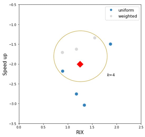
Figure 2.
Illustration of the k-NN classifier method to predict the type of regression (uniform or inverse-distance weighting), used by Algorithm 3. Red diamond: target site. The circles group the k = 4 nearest neighbors in the 2-dimensional space created by the features speedup and RIX. The same idea holds for predicting the number of neighbors .
To determine which of the k-NN classifiers evaluated in Algorithm 3 had the best performance, wind speed predictions were conducted using the predicted hyperparameters and . The classifier minimizing the average error of the reference sites (leaving out the target site) was selected. Each site at its turn was assumed to be a target site, therefore (number of sites) average errors were calculated; the classifier that repeated the most in those performance rankings was then selected. A pseudocode description of the method described is shown in Algorithm 4.
| Algorithm 4k-NN regression to estimate using estimated hyperparameters |
|
2.2.2. Hyperparameter Selection and Testing through Nested Cross-Validation
As described above, often k-NN methods deals with time series data, which portray different characteristics when analyzed within different periods. For hyperparameter tuning and providing an unbiased validation of a given method for modeling or predicting a variable (such as wind speed), cross-validation is commonly carried out. In the present work, the nested cross-validation approach illustrated in Figure 3 was implemented. With such an approach, the testing period (green square in Figure 3) appears chronologically after the training period (blue squares). The training data are used to systematically evaluate the number of neighbors and type of regression, and the setup that minimizes the MPE is selected and used in the testing set to provide an unbiased measure of the model prediction error. By repeating this process with multiple testing sets, a better estimate of model performance is obtained. In this work, the data set was split into five nested subsets, using the setup shown in Table 1. The testing period was constant in all runs (2 months). As mentioned before, this implementation was conducted for reference purposes only.
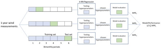
Figure 3.
Illustration of the nested hyperparameter estimation and cross-validation approach.

Table 1.
Setup of nested cross-validation simulations.
2.3. Feature Selection for k-NN Methods
A number of features were considered for their use with k-NN-based methods. A basic requirement for all candidates was the possibility of calculating their values for each location of interest from geographic information alone, in a completely analogous way in which flow modeling tools such as WAsP or WindSim construct wind maps for a site or region of interest. The following feature candidates were found to be suitable candidates:
- The terrain ruggedness index RIX. Although the RIX correction procedure [] did not provide a significant improvement of the WAsP flow modeling results for the site, a weak correlation between the WAsP flow modeling error for the wind speed indicated a possible suitability of the RIX index as a similarity feature.
- The orography-induced speedup (e.g., relative increase in wind speed due the terrain slope). A modest correlation between the prediction error and the difference between the WAsP-calculated topography-induced speedups was found (Figure 4), indicating that the speedup is a possible similarity measure candidate.
- The distance between measurement locations (met towers). As shown in Figure 4, the distance between locations bears a similar impact on the flow modeling results as the difference between speedup values.
- The vertical wind shear. The wind shear was found to have a significant (negative) correlation with the prediction error, and was therefore expected to be among the important predictor variables of the k-NN method. Note that the degree of correlation between the flow modeling error and the feature candidates shown in Figure 4 does not have any impact on the k-NN methodology, beyond the decision of including or not a given candidate feature in the list of k-NN predictors. The k-NN method determines the optimal set of predictors in an automated fashion, as described above.
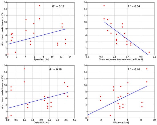
Figure 4.
Mean absolute modeling error for WAsP-predicted wind speed vs. features selected for the k-NN study. The dots correspond to the cross-validation between each pair of sites. The blue line represents the linear regression of the errors as a function of presented features.
The following additional feature parameters were used for the assessment of power density:
- The Weibull scale and shape parameters. Determining Weibull parameters requires on-site measurements (or simulated winds from atmospheric models) for at last one location. Using such a reference location, a transferred wind rose (the latter understood as the set of angular wind speed histograms) can be constructed using a wind flow modeling tool. Since local flow conditions are different for different wind directions, the average transferred wind rose will generally have different Weibull parameters.
- The -value, or coefficient of determination, of the Weibull fit. The transfer of wind roses may not only change the Weibull parameters, but may also distort the underlying histogram, resulting in varying degrees of goodness of fit. -related parameters can be constructed for their use as similarity features; additionally, a modified weighting scheme (similarly to the one proposed in []) was explored as well, where the -value was used to build a confidence level matrix as part of a generalized inverse-distance averaging scheme.
2.4. Setup of the k-NN Simulations
The current work consists of the following sequence of assessments:
- (1)
- KNN0. All available wind speed data for the full one-year period (see Section 2.5) were used to perform a k-NN regression for each of the five towers as target site. The optimal hyperparameters and were calculated from the full regression. Algorithms 1 and 2 were used for this purpose. This is a baseline case, constructed for reference purposes.
- (2)
- KNNa. In order to conduct an independent test of the methodology, the optimal hyperparameters were estimated from all towers, excluding the target tower itself. The corresponding procedure is described in Algorithm 3.
- (3)
- KNNb. Instead of using the measured wind speed information directly as a predictor for a given target site, an alternative method consists of using the WAsP predictions for the target site, prepared with each of the predictor sites. The same set of features and feature combinations as before were used in this step.
- (4)
- KNNc. Since methods KNNa (driven exclusively with observed wind speed data) and KNNb (working on WAsP-processed observational data) represent independent assessments, an ensemble version was performed, where methods KNNa and KNNb were combined linearly.
- (5)
- KNNd. For an independent validation of the k-NN approach, an additional method was implemented, where optimal hyperparameters were determined and validated in the nested approach described in Section 2.2.2.
2.5. Validation Data
On-site tall tower meteorological data from the development phase of a commercial wind farm in Mexico were used for model construction and validation. The data are proprietary and are not in the public domain. Each of the five towers at the site (“site B”) was equipped with three pairs of redundant cup anemometers (class I for primary sensors, standard for redundant) placed at 80, 60, and 40 m above ground level. The wind direction was measured at two levels (42 and 78 m). Temperature measurements were taken at 12 and 80 m above ground level. Data were recorded at 10 min intervals; for each variable, the mean, maximum, minimum and standard deviation were recorded. One full year of concurrent information with only minor data gaps was selected to avoid seasonal biases. Initial quality assurance was conducted in a semi-automatic way using Windographer. Overall data recovery after quality assurance was 99.9%. All reported results for the wind speed modeling accuracy in this study refer to the 80 m wind speed.
In order to build a continuous observational period, three reconstruction methods were used: (1) replacement of missing or invalid 80 m data with those from the redundant sensor, prior tower shadow correction when necessary; (2) vertical extrapolation, and (3) principal component analysis (PCA). Vertical extrapolation was used when 40 m and 60 m wind speed data were available. PCA was used to take advantage of concurrent data from other towers where no concurrent wind speed data at the same tower were available.
In order to ascertain that the reconstructed continuous data records for each met tower were statistically indistinguishable from the quality-controlled original data, both a test for the observed () and reconstructed () wind speed distributions, with , and a Kolmogorov–Smirnov test for the cumulative probability density functions ( and , respectively) were conducted. All tower measurements at site B successfully passed both tests, demonstrating that the quality-controlled original data sets and the reconstructed full data sets were statistically indistinguishable.
The wind regime at the site is essentially bi-modal, with Southerly winds predominating most of the year, the remainder corresponding to Northerly winds (see Figure 5). All towers were located at either the Southern or the Northern edge of a plateau structure, with three towers (S01_B, S02_B, SO3_B) being located at the Southern and two (S04_B, S05_B) at the Northern edge. S01_B and S05_B are somewhat more exposed locations, sitting on extruded portions of the plateau, whereas the other towers sit between a steep slope and the flat upper part of the plateau.
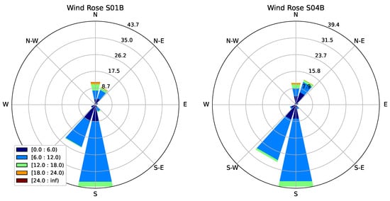
Figure 5.
Wind rose observed at sites S01B and S04B from June 2016 to June 2017.
2.6. Flow Modeling: WAsP
WAsP [] was used for (1) wind flow modeling and cross-prediction of the wind resource at all locations with observational data; and (2) the determination of the feature parameters (Section 2.4). Orography inputs come from the Shuttle Radar Topography Mission (SRTM) digital elevation data [] with a resolution of 1 arcsec (30 m). The SRTM 1 Arc-Second Global version [] used was downloaded from the U.S. Geological Survey (USGS) website. The domain extends 10 km beyond the limits of the site of interest in order to create a large enough buffer to avoid boundary effects; contour lines with a spacing of 10 m were used. The GlobeLand30 (GLC30) database [] with a resolution of 1 arcsec (30 m) was used to create a roughness map. Using the GLC30 version 2020 database improves the cross-validation results for the wind speed compared to using the WAsP default database (GlobCover-2009 map []); therefore, we use the former roughness data hereafter. A detailed discussion of the impact of potentially more accurate roughness maps and its impact of flow modeling accuracy is not part of the present work.
In the WAsP modeling chain, the observed wind is generalized using predefined heights and roughness lengths, which can be modified. It was observed that a fine tune of these values reduces the error in the predicted wind. Here, the predefined heights were set to 10, 30, 60, 80 and 100 m above ground level and the standard roughness lengths were set to 0.0, 0.05, 0.11, 0.23 and 0.5 m.
In order to account for atmospheric stability, a systematic assessment of the heat flux impact on the vertical wind shear profiles was conducted (not shown). By using the WAsP default configuration, corresponding to a slightly stable condition with a heat flux offset of W/m, a good fit with the observed profiles was found at all tower locations. Allowing for heat flux offset variations did not improve the results. Another option in the WAsP software is the geostrophic shear model, which is turned on by default. The geostrophic shear is obtained from coarse reanalysis data, which cannot resolve the slopes in mountainous terrain [], and can therefore give unphysically large geostrophic wind shear values. This was also observed for the study site in this work (0.02 m/s/m). The model was therefore turned off in all cases.
An attempt to further improve the results of the cross-validation predictions using the delta-RIX methodology [] was performed. However, as mentioned in Section 2.3, no statistically significant improvement was obtained.
As an additional reference, the WAsP software was run in (RANS) CFD mode; the results were found to be similar to the ones obtained with WindSim, discussed in the next subsection. Unless mentioned otherwise, all WAsP results were obtained with the standard (linear) flow solver.
2.7. Flow Modeling: WindSim
A RANS-based solver, the commercial software package WindSim ([]), was used in an attempt to improve cross-predictions, given the terrain complexity of the site. The same topography data (STRM and GLC30) as those in WAsP were used. The WindSim mesh was setup with an initial horizontal resolution of 50 m in the refinement area for convergence and initial performance tests; the resolution in the refinement area used in the final selected configuration was then set to 20 m for a better representation of the terrain at its steep parts. Setup parameters for WindSim include (1) a toggle parameter for including the forest model (on/off); (2) the free parameters of the forest model; (3) the turbulence closure model (k- or k-); and (4) the type of atmospheric stability. A Taguchi experiment design [] was set up in order to assess the different free parameters of the forest model. The assumption of neutral stability was found to produce a good agreement with the observed wind speed profiles; moreover, simulations under stable and unstable conditions lead to convergence problems, so only neutral stability conditions were considered for the final model setup. The use of the k- turbulence closure model and the omission of the forest model produce the best results generally, so we use this configuration hereafter. A detailed discussion of the setup, experiment design and results obtained with the WindSim study are beyond the scope of the present work and will be reported elsewhere.
3. Results
3.1. Cross-Validation with Flow Models
As baseline, we choose the best results from WAsP and WindSim, which are summarized in Figure 6, where the cross-validation errors (in %) for the prediction of the average wind speed obtained with WAsP (a) and WindSim (b) are shown. In both cases, a relatively small prediction error is observed within groups S (S01B, S02B, S03B), which are locations at the Southern edge of the plateau, and N (S04B, S05B), which are at the Northern edge. The error is dramatically larger when cross-predicting between these two groups. WindSim does not seem to systematically reduce the latter errors.
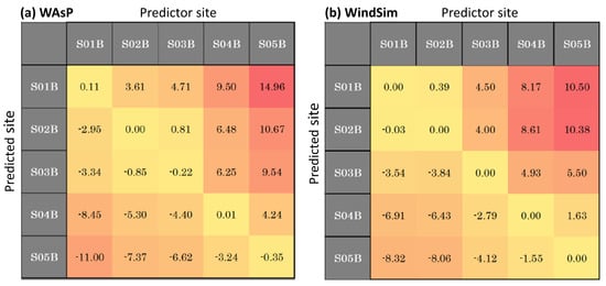
Figure 6.
Cross−validation errors for the prediction of the average wind speed in % obtained with WAsP (a) and WindSim (b). Light orange colors: small errors; reddish colors: large errors.
Figure 7 shows the cross-validation results as a function of the distance between predictor-predicted pairs. This distance highly influences the prediction accuracy, but only within the northern (N) and southern (S) zones. The absolute prediction errors are similar within the zones. However, inter-zone cross-predictions show a much larger error than intra-zone cross-predictions. This is as expected, as the met towers are located near either of the plateau edges. WindSim demonstrated good results in the Bolund benchmark [], so one might expected improvements compared to WAsP at this site. WindSim results are only slightly better than WAsP and both models show (≈10%) errors when cross-predicting between zones.
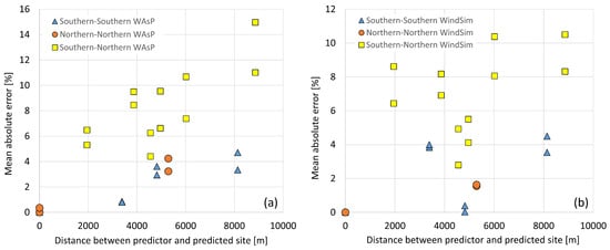
Figure 7.
Absolute mean prediction error of the cross-validations as a function of distance and zone for the results using (a) WAsP; and (b) WindSim.
Based on the above findings, which indicate that the cross-prediction accuracy between zones is limited, we can assume that the wind climatology at the S and N edges of the plateau is significantly influenced by the local orography. Using an inverse-distance weight approach does not improve cross-predictions as shown in Table 2 (column 3) for the case of WAsP. The lack of accuracy continues to be particularly noticeable at the edges of the plateau (locations S01B and S05B), where the wind speed errors are of the order of 7–8%, which are much larger than the accepted error for wind farm development.
Table 2.
Percentage error of the cross-predictions of four implementations of the k-NNa method (kNNa card. 2 − 5) operating for cardinalities 2, 3, 4 and 5, compared to the flow modeling results using WAsP. WAsP = average of all WAsP cross-predictions for a given target met tower site; IDW = inverse-distance averaged WAsP cross-predictions.
3.2. k-NN Modeling Results
3.2.1. Overall Results
As described in Section 2.4, the kNNa model uses estimated, rather than fitted, hyperparameters, and therefore provides a true prediction of the wind speed at each location, as opposed to a fit to the data. Input data are the measured wind speeds at each of the towers, excluding those of the target location. As shown in Table 2, where the results for four implementations (see Section 2.2.1) of the kNNa method are shown, alongside the results from WAsP, the overall performance of the k-NN method is far better than that of the flow model. Whereas the uniformly (column 2) and inverse-distance weighted (column 3) average WAsP results have an error of about 5%, the k-NN error is about 1.5%, with the best-ranking method (kNNa.card4, using cardinality 4, see Table 3) yielding an error of only 1.29%.
Table 3.
Highest-ranking k-NN solutions for case kNNa and each cardinality (number of features considered). Estimated optimal hyperparameters and are shown, along with their feature sets and their mean percentage error for each target site.
It is also worth noting that not only is the average error of the k-NN predictions significantly smaller than the one obtained with WAsP, but the discrepancies at the more exposed locations are also largely resolved. While the flow model produces deviations of about 8 and % for S01B and S05Bs, respectively, the corresponding k-NN results are around 3.75 and 0.5%, respectively.
3.2.2. Hyperparameter Optimization
In order to build some intuition of the structure of the results of the k-NN method, the KNNa case described above will be further discussed. As described above, KNNa uses estimated hyperparameters ( and ) for each target site, rather than their optimal values (as determined by method KNN0). The modeled wind speeds are therefore independent predictions, not the result of a regression. The results are shown in Table 3 for each target site and each level of cardinality. The method with cardinality 4 (based on features’ distance, RIX, shear exponent, and time) produces the smallest error (1.29% average), though good results are obtained with the other methods as well. In all cases, the error is much smaller than in the case of the flow modeling predictions (WAsP or WindSim). It can also be seen that the number of nearest neighbors () used for the prediction of the wind speed at each location varies among methods. Whereas the cardinality-2 method requires up to nine nearest neighbors and shows great variability in the hyperparameter among sites, the results for the cardinality-4 method appear to be more consistent among the tower locations for both and , with the best predictions for each location based on one or two adjacent locations and using uniform weighting in all cases. To understand why a location can have nine neighbors in a five-tower arrangement, it should be recalled that time is used as a feature parameter as well, allowing the wind speed at time step to be modeled based on wind speeds at times and . It should also be stressed that the aim is to predict wind speeds and not to forecast them (in time), which would preclude future time steps to be considered. In any case, restricting predictor wind speeds to simultaneous time steps still only produces excellent results, as evidenced by the cardinality-3 and -4 methods, with method 3 being the highest-ranking method of all.
3.2.3. Results Obtained the Hybrid WAsP-KNN Approach
Here, we first predict the wind speed at a location (e.g., by using WAsP) and then we use these predictions at the target location from each predictor site within the k-NN model framework. In other words, this implementation works with the transferred climatologies, rather than with the measured wind speed time series.
Results obtained with this method (referred to as KNNb in Section 2.4) are shown in Table 4 under the column tagged “hybrid”. The method does not result in a decrease in the error at the more exposed locations (S01B and S05B), although a slight improvement at the less exposed locations occurs. The MAPE is comparable to that of WindSim.
Table 4.
Summary of all wind speed modeling results in this work.
3.2.4. Results Obtained with the Ensemble Approach
The ensemble approach (kNNc) consists of a linear superposition of models kNNa and kNNb, where kNNa is driven by the observed wind speed data at each location, and kNNb works on the transferred microclimates from each predictor tower to the target location.
In order to determine the statistical weight of each method, first a regression was conducted, leading to optimal weights for each target site. In a second step, average weights were used to build a new prediction. The accuracy observed was somewhat better on the average (around 1.1%) than the observational data-based k-NN results, and showed a better consistency among target sites. Since the two methods used (kNNa and kNNb) are independent predictions of the wind resource, as their combination can lead to errors being canceled out—as shown in Table 4, where the average error is about 1%, with a quite homogeneous prediction accuracy at all locations.
3.2.5. Results Obtained with the Nested Approach
The nested approach (kNNd) cannot be directly used to estimate the wind resource at a location without on-site measurements (as opposed to methods kNNa, kNNb, and kNNc) and was implemented for reference purposes only. Given that kNNd uses the full set of data, the metrics of kNNd are very good, with an average error of about 1%, comparable to the best performing methods kNNa and kNNb. Note that kNNd does a better job at locations (S02B, S03B, SOB) compared to the more exposed locations (S01B and S05B), similarly to kNNa and kNNb, highlighting that the capabilities of a method based on similarity are limited by the number of locations available with similar features. In modern wind resource campaigns, which now often include remote sensing devices such as sodar [] or lidar [], this limitation can, however, readily be overcome with complementary remote sensing campaigns.
3.2.6. Power Density Results
As described above, estimating power density is potentially more challenging in a complex terrain than estimating wind speed because considerable differences may arise in the simulated wind speed distributions due to terrain effects. As shown in Table 5, the WAsP predictions for power density had similar errors at four locations and a large error (27%) at one location (S01B). At this location, the wind speed prediction of both WAsP and k-NN methods (see Table 5) had also a large error. As this more exposed location, the simulated wind speed distribution differs the most from the observations.
Table 5.
Average percentage error for the prediction of power density obtained with WAsP (linear solver), the original implementation of the k-NN method, tuned for wind speed prediction, and a modified k-NN version, optimized for the prediction of the power density. The four highest ranking implementations are shown for both k-NN cases.
As shown in Table 5, the k-NN method (optimized for wind speed prediction) does a considerably better job of predicting power density at SO1B than WAsP (albeit at the expense of worse predictions for S05B), resulting in similar overall errors for the set of five towers as in the case of WAsP. However, by including the location-specific Weibull parameters as additional similarity features, the k-NN method can be tuned to provide significantly better power density predictions, as shown in columns 7–10 of Table 5. Prediction errors are now down by approximately 10% for location S01B and on average by only approximately 3 to 3.5% for all sites, which is only half of the error obtained with WAsP.
4. Summary and Conclusions
Here, a novel method for the modeling of the wind resource with improved accuracy was proposed and evaluated using on-site data from a site with complex terrain characteristics. As opposed to industry-standard approaches, which mainly rely on flow models, the new method uses a simple and intuitive machine learning algorithm, based on the k-nearest neighbors concept. While being a consolidated method in the literature on advanced statistical modeling and machine learning, to the best knowledge of the authors, no such approach was previously proposed or demonstrated in the field of wind resource assessment.
The k-NN method in this work was based on the concept of similarity between met tower locations. To assess similarity, the method uses classifiers or features of each location. Features related to the terrain characteristics, flow-related quantities and micro-climate parameters were selected. All location features can be readily obtained with a microscale flow model. All k-NN runs performed in this work use features generated with WAsP. In order to generate a baseline for comparisons, cross-validations between the five tall (80 m) tower locations were conducted with both WAsP (using its linear flow solver) and WindSim (using a RANS implementation). Both software suites were fine-tuned in order to strive for optimal performance.
Given that all met towers are located at edge locations, a clear improvement of the RANS-CFD predictions over the linear flow model was expected. Some improvement by the best-tuned RANS model was indeed observed. Both flow models failed, however, to accurately transfer the measured climatologies from the northern edge to the southern edge locations and vice versa with the accuracy required by modern competitive wind farms.
Four conceptually different k-NN approaches were proposed and assessed, with one of the methods (kNNd) being used for reference purposes. The baseline model (kNNa) works directly with the quality-controlled wind speed or power density 10 min time series retrieved from all met towers other than the target location used for validation. The hyperparameters required by the k-NN model were estimated with a novel methodology based on the similarity between locations, which takes advantage of the full observational period. This is somewhat different from a typical machine-learning approach (implemented as method kNNd) and more suitable for the context of this work.
Two other variants of the k-NN concept were implemented as well. In kNNb, the observed wind data were first transferred to the target site using WAsP, and the k-NN method was then applied to those transferred climatologies. This hybrid approach has the advantage of being an independent assessment of the wind resource at the target site, allowing for the construction of an ensemble method (kNNc) by combining the predictions of kNNa and kNNb.
The k-NN concept, in its different implementations, provided significant improvements overflow modeling results. While the average WAsP prediction accuracy was around 5% for the wind speed and 7% for the wind power density, the corresponding figures for k-NN method were only approximately 1.5 and 3%, respectively. It should be noted that from the perspective of a wind resource modeler, the k-NN method works similarly to a flow model such WAsP or WindSim; only terrain-related information and wind time series for different measurement locations are needed.
While providing improved accuracy over wind flow models, the k-NN approach does have some limitations. First, a flow model is needed to determine the feature parameters of each location of interest. Therefore, the k-NN method can be viewed as an add-on to existing wind modeling suites such as WAsP and WindSim, rather than a stand-alone method. However, wind resource modelers typically have access to flow modeling tools, so this is not a practical limitation. Second, the k-NN method needs more than one measurement location, as opposed to WAsP or WindSim. This is, however, not a strong limitation, since nowadays, a number of met towers are routinely installed at prospective wind farm sites, and additional measurement locations can be created dynamically using remote sensing devices such as lidar and sodar. The proposed method was therefore believed to have good prospects for applications in a practical wind resource assessment context.
Author Contributions
Conceptualization, J.L.P. and O.P.; data curation, P.Q.-N. and G.C.-F.; formal analysis, P.Q.-N., J.L.P. and O.P.; funding acquisition, A.P. and O.P.; investigation, P.Q.-N. and G.C.-F.; methodology, P.Q.-N., J.L.P. and O.P.; project administration, A.P. and O.P.; resources, A.P. and O.P.; software, R.F. and G.C.-F.; supervision, J.L.P. and O.P.; validation, R.F.; visualization, P.Q.-N.; writing—original draft, O.P.; writing—review and editing, P.Q.-N., R.F., A.P., G.C.-F. and O.P. All authors have read and agreed to the published version of the manuscript.
Funding
This research was funded by the Danish International Development Agency under grant number 17-M01-DTU.
Informed Consent Statement
Not applicable.
Acknowledgments
This work was partly funded by the Ministry of Foreign Affairs of Denmark and administered by the Danida Fellowship Centre through the ‘Multi-scale and model-chain Evaluation of Wind Atlases’ (MEWA) project. P.Q. acknowledges a tuition waver for M.Sc. studies from Tecnológico de Monterrey, as well as a stipend from CONACYT (Mexico). O.P. and G.C.-F. appreciate support from the institutional research group on Energy and Climate Change at Tecnológico de Monterrey. J.L.P. is grateful to the institutional research group on Data Science and Optimization at Tecnológico de Monterrey. All authors acknowledge the wind resource data from an undisclosed wind project developer, without which, this study would not have been possible.
Conflicts of Interest
The authors declare no conflict of interest.
Nomenclature
| The cardinality of the set x | |
| The estimated type of regression | |
| The estimated number of neighbors | |
| The estimated variable (uniform weighted regression) | |
| The estimated variable (inverse distance weighted regression) | |
| The set of all possible combination of features | |
| The mean of the variable x | |
| The matrix of mean predictor values | |
| The vector of mean predictor values at site | |
| The standard deviation of the variable x | |
| c | The type of regression either uniform weighting or inverse distance weighting |
| The optimal type of regression | |
| The set of features | |
| K | The maximum number of neighbors |
| k | The number of neighbors |
| The optimal number of neighbors | |
| The norm or Euclidean distance | |
| The mean percentage error | |
| The MPE obtained from a inverse distance weighing regression | |
| The MPE obtained for a given site from a set of features and k number of neighbors | |
| N | The number of observations |
| The number of features | |
| The set of nearest neighbors to the site | |
| The set of sites to be predicted | |
| w | The weight of the regression either one or calculated with the inverse distance |
| X | The matrix of predictors |
| The target site | |
| The observed variable to be predicted at a time step i |
References
- Lazard’s Levelized Cost of Energy and Storage, v14. 2020. Available online: https://www.lazard.com/perspective/lcoe2020 (accessed on 14 March 2021).
- Williams, J.H.; Jones, R.A.; Haley, B.; Kwok, G.; Hargreaves, J.; Farbes, J.; Torn, M.S. Carbon-Neutral Pathways for the United States. AGU Adv. 2021, 2, e2020AV000284. [Google Scholar] [CrossRef]
- Buira, D.; Tovilla, J.; Farbes, J.; Jones, R.; Haley, B.; Gastelum, D. A whole-economy Deep Decarbonization Pathway for Mexico. Energy Strategy Rev. 2021, 33, 100578. [Google Scholar] [CrossRef]
- Bompard, E.; Grosso, D.; Huang, T.; Profumo, F.; Lei, X.; Li, D. World Decarbonization through Global Electricity Interconnections. Energies 2018, 11, 1746. [Google Scholar] [CrossRef] [Green Version]
- Mortensen, N.G. Wind Resource Assessment Using the WAsP Software Department of Wind Energy E Report 2019. 2018, p. 45. Available online: https://backend.orbit.dtu.dk/ws/portalfiles/portal/164389714/Wind_resource_assessment_using_the_WAsP_software_DTU_Wind_Energy_E_0174_.pdf (accessed on 17 July 2021).
- Beaucage, P.; Brower, M.C.; Tensen, J. Evaluation of four numerical wind flow models for wind resource mapping. Wind Energy 2014, 17, 197–208. [Google Scholar] [CrossRef]
- Spyridonidou, S.; Vagiona, D.G. Systematic Review of Site-Selection Processes in Onshore and Offshore Wind Energy Research. Energies 2020, 13, 5906. [Google Scholar] [CrossRef]
- Gomes Da Silva, A.F.; Peña, A.; Hahmann, A.N.; Zaparoli, E.L. Evaluation of two microscale flow models through two wind climate generalization procedures using observations from seven masts at a complex site in Brazil. J. Renew. Sustain. Energy 2018, 10. [Google Scholar] [CrossRef] [Green Version]
- Palma, J.M.; Castro, F.A.; Ribeiro, L.F.; Rodrigues, A.H.; Pinto, A.P. Linear and nonlinear models in wind resource assessment and wind turbine micro-siting in complex terrain. J. Wind Eng. Ind. Aerodyn. 2008, 96, 2308–2326. [Google Scholar] [CrossRef]
- Bechmann, A.; Sørensen, N.N.; Berg, J.; Mann, J.; Réthoré, P.E. The Bolund Experiment, Part II: Blind Comparison of Microscale Flow Models. Bound. Layer Meteorol. 2011, 141, 245–271. [Google Scholar] [CrossRef] [Green Version]
- Hristov, Y.; Oxley, G.; Agar, M. Improvement of AEP predictions using diurnal CFD modelling with site-specific stability weightings provided from mesoscale simulation. J. Phys. Conf. Ser. 2014, 524. [Google Scholar] [CrossRef] [Green Version]
- Veronesi, F.; Grassi, S.; Raubal, M.; Hurni, L. Statistical learning approach for wind speed distribution mapping: The uk as a case study. Lect. Notes Geoinf. Cartogr. 2015, 217, 165–180. [Google Scholar] [CrossRef]
- Foresti, L.; Tuia, D.; Kanevski, M.; Pozdnoukhov, A. Learning wind fields with multiple kernels. Stoch. Environ. Res. Risk Assess. 2011, 25, 51–66. [Google Scholar] [CrossRef] [Green Version]
- Lawan, S.M.; Abidin, W.A.; Masri, T. Implementation of a topographic artificial neural network wind speed prediction model for assessing onshore wind power potential in Sibu, Sarawak. Egypt. J. Remote Sens. Space Sci. 2020, 23, 21–34. [Google Scholar] [CrossRef]
- Tang, X.Y.; Stoevesandt, B.; Fan, B.; Li, S.; Yang, Q.; Tayjasanant, T.; Sun, Y. An on-site measurement coupled CFD based approach for wind resource assessment over complex terrains. In Proceedings of the I2MTC 2018—2018 IEEE International Instrumentation and Measurement Technology Conference: Discovering New Horizons in Instrumentation and Measurement, Houston, TX, USA, 14–17 May 2018; pp. 1–6. [Google Scholar] [CrossRef]
- Bechmann, A.; Leon, J.P.M.; Olsen, B.T.; Hristov, Y.V. The most similar predictor—On selecting measurement locations for wind resource assessment. Wind Energy Sci. 2020, 5, 1679–1688. [Google Scholar] [CrossRef]
- Shabani, S.; Samadianfard, S.; Sattari, M.T.; Mosavi, A.; Shamshirband, S.; Kmet, T.; Várkonyi-Kóczy, A.R. Modeling Pan Evaporation Using Gaussian Process Regression K-Nearest Neighbors Random Forest and Support Vector Machines; Comparative Analysis. Atmosphere 2020, 11, 66. [Google Scholar] [CrossRef] [Green Version]
- Mortensen, N.G.; Rathmann, O.; Tindal, A.; Landberg, L. Field validation of the ΔRIX performance indicator for flow in complex terrain. In Proceedings of the European Wind Energy Conference and Exhibition 2008, Brussels, Belgium, 31 March–3 April 2008; Volume 1, pp. 186–204. [Google Scholar]
- Toledo, C.; Chávez-Arroyo, R.; Loera, L.; Probst, O. A surface wind speed map for Mexico based on NARR and observational data. Meteorol. Appl. 2015, 22, 666–678. [Google Scholar] [CrossRef]
- Farr, T.; Rosen, P.; Caro, E.; Crippen, R.; Duren, R.; Hensley, S.; Kobrick, M.; Paller, M.; Rodriguez, E.; Roth, L.; et al. Shuttle Radar Topography Mission: Mission to map the world. Rev. Geophys. 2008, 45, 3–5. [Google Scholar] [CrossRef]
- Earth Resources Observation Furthermore, Science (EROS) Center. Shuttle Radar Topography Mission (SRTM) 1 Arc-Second Global. 2017. Available online: https://doi.org/10.5066/F7PR7TFT (accessed on 17 July 2021).
- Jun, C.; Ban, Y.; Li, S. Open access to Earth land-cover map. Nature 2014, 514, 434. [Google Scholar] [CrossRef] [PubMed] [Green Version]
- Bontemps, S.; Defourny, P.; Bogaert, E.V.; Kalogirou, V.; Perez, J.R. GLOBCOVER 2009 Products Description and Validation Report. ESA Bull. 2011, 136, 53. [Google Scholar]
- Floors, R.R.; Troen, I.; Kelly, M.C. Implementation of Large-Scale Average Geostrophic Wind Shear in WAsP12.1. 2018, p. 11. Available online: https://backend.orbit.dtu.dk/ws/portalfiles/portal/149165080/e_report_0169.pdf (accessed on 17 July 2021).
- WindSim. Available online: http://windsim.com/ (accessed on 13 March 2021).
- Rout, A.; Sahoo, S.S.; Singh, S.; Pattnaik, S.; Barik, A.K.; Awad, M.M. Chapter 7—Benefit-cost analysis and parametric optimization using Taguchi method for a solar water heater. In Design and Performance Optimization of Renewable Energy Systems; Assad, M.E.H., Rosen, M.A., Eds.; Academic Press: Cambridge, MA, USA, 2021; pp. 101–116. [Google Scholar] [CrossRef]
- Chávez-Arroyo, R.; Gómez, H.; Herbert, F.J.; Romo Perea, A.; Probst, O. Mesoscale modeling and remote sensing for wind energy applications. Rev. Mex. Física 2013, 59, 114–129. [Google Scholar]
- Basse, A.; Pauscher, L.; Callies, D. Improving Vertical Wind Speed Extrapolation Using Short-Term Lidar Measurements. Remote Sens. 2020, 12, 1091. [Google Scholar] [CrossRef] [Green Version]
Publisher’s Note: MDPI stays neutral with regard to jurisdictional claims in published maps and institutional affiliations. |
© 2021 by the authors. Licensee MDPI, Basel, Switzerland. This article is an open access article distributed under the terms and conditions of the Creative Commons Attribution (CC BY) license (https://creativecommons.org/licenses/by/4.0/).