
Improvement of Stand-Alone Solar PV Systems in the Maputo Region by Adapting Necessary Parameters


Abstract
:1. Introduction
2. Analysis of Installation and Operating Parameters of Solar PV Systems
3. Solar PV Power Output
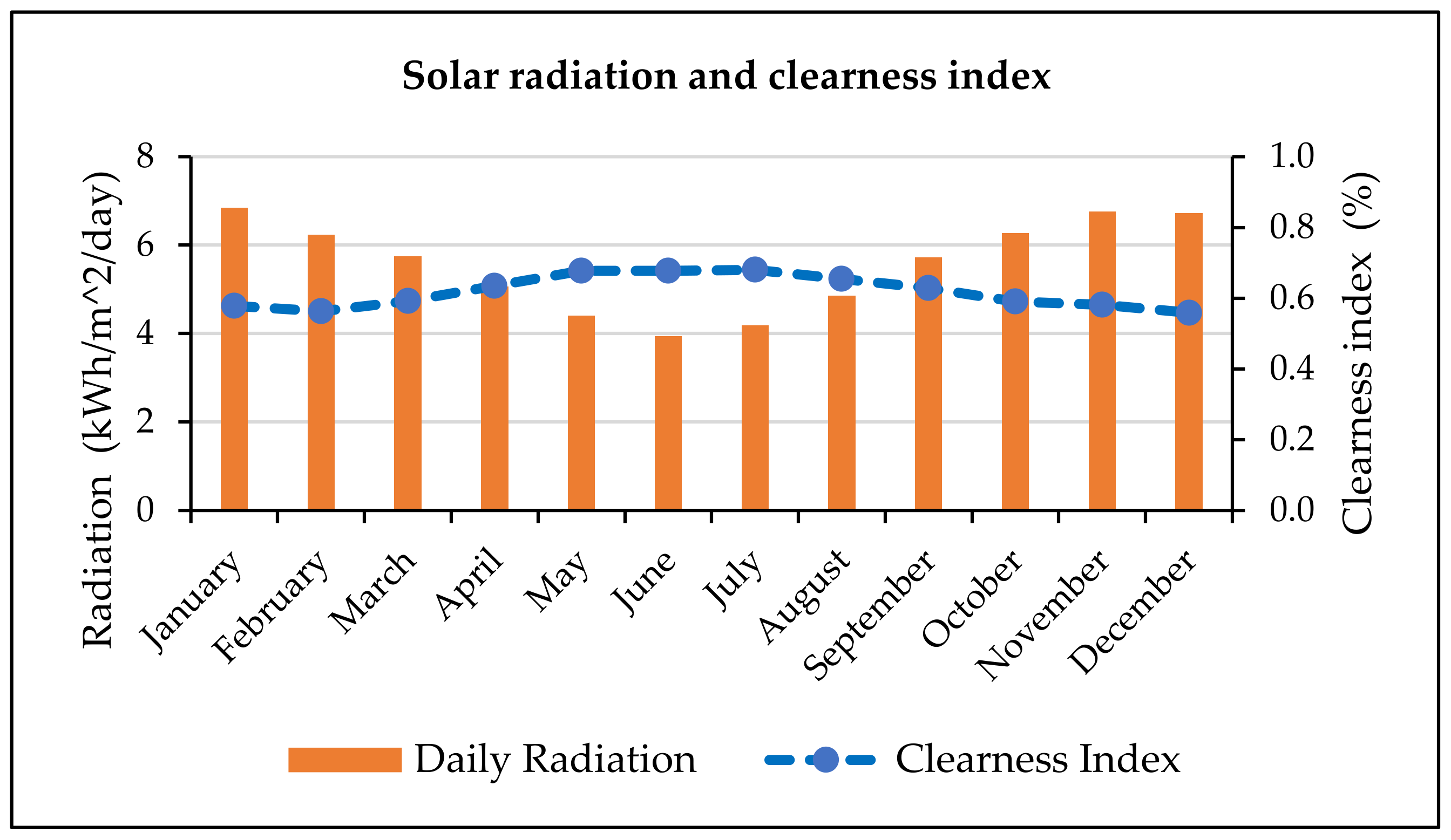
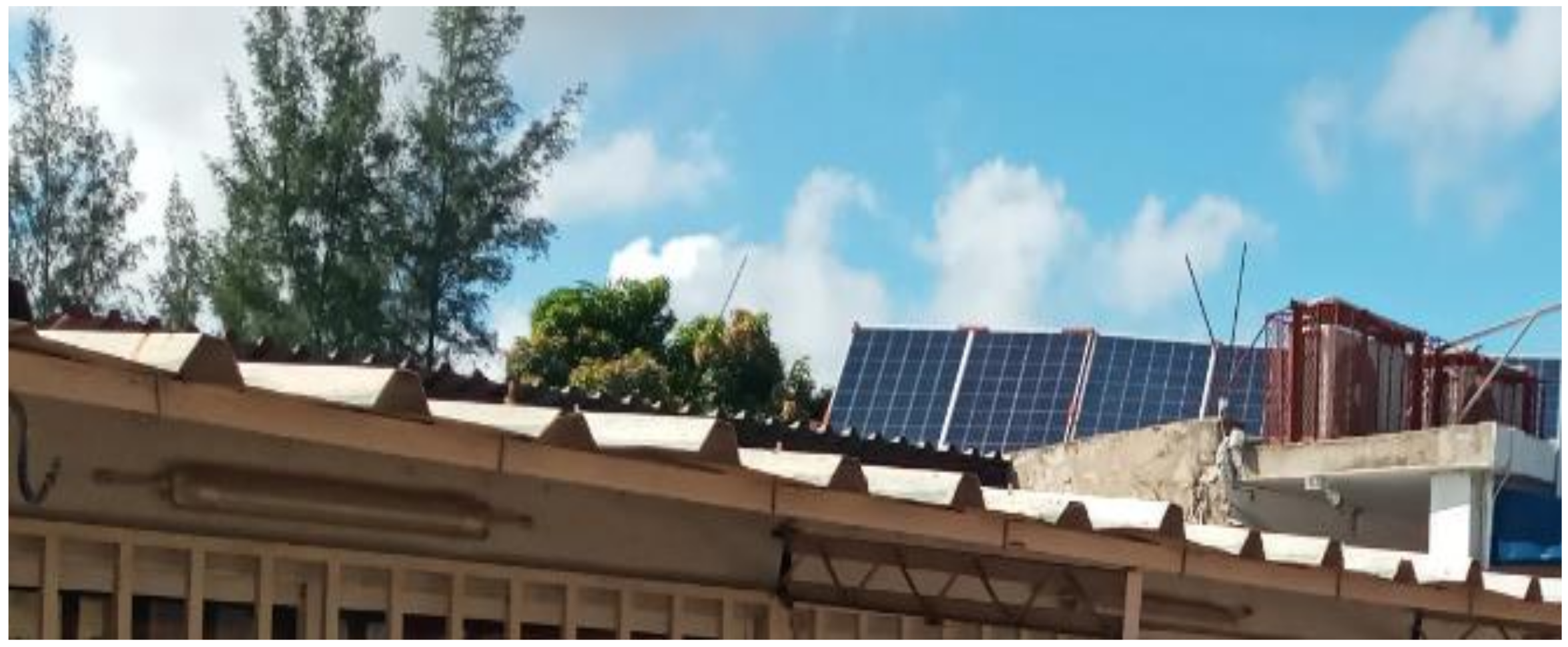
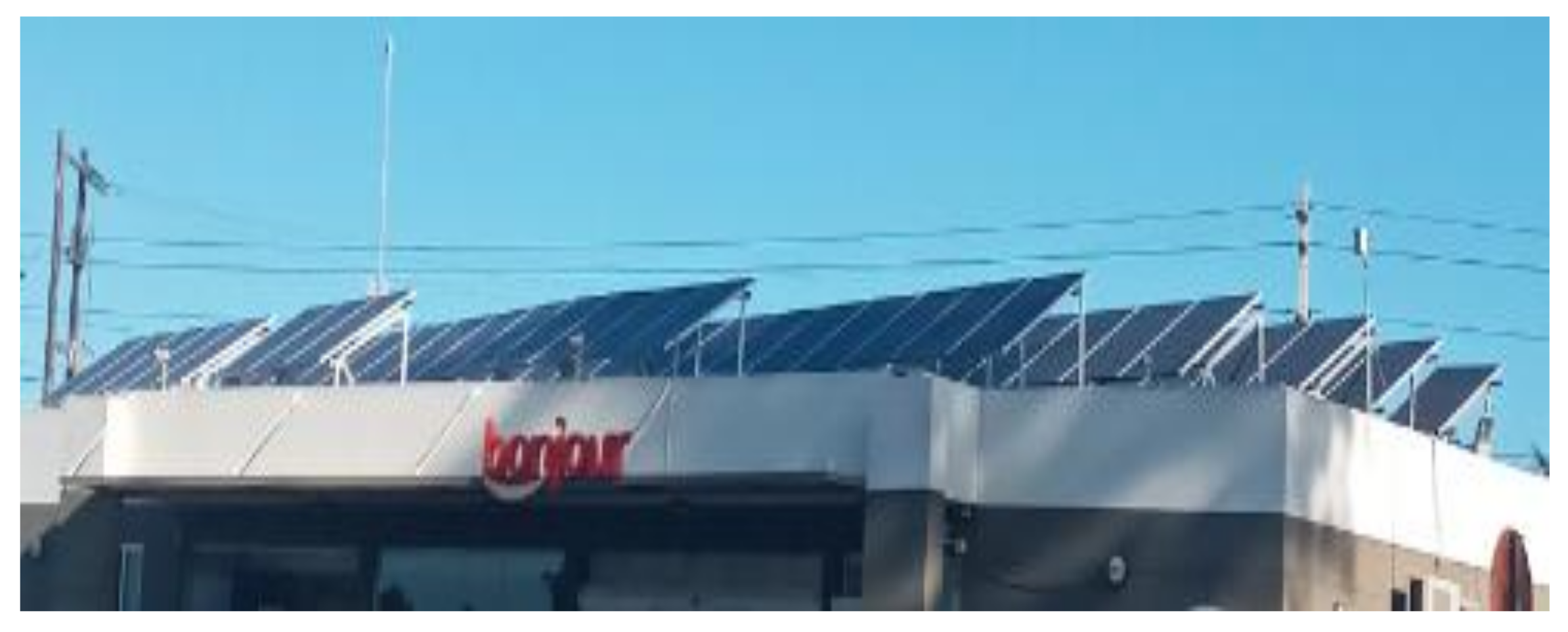
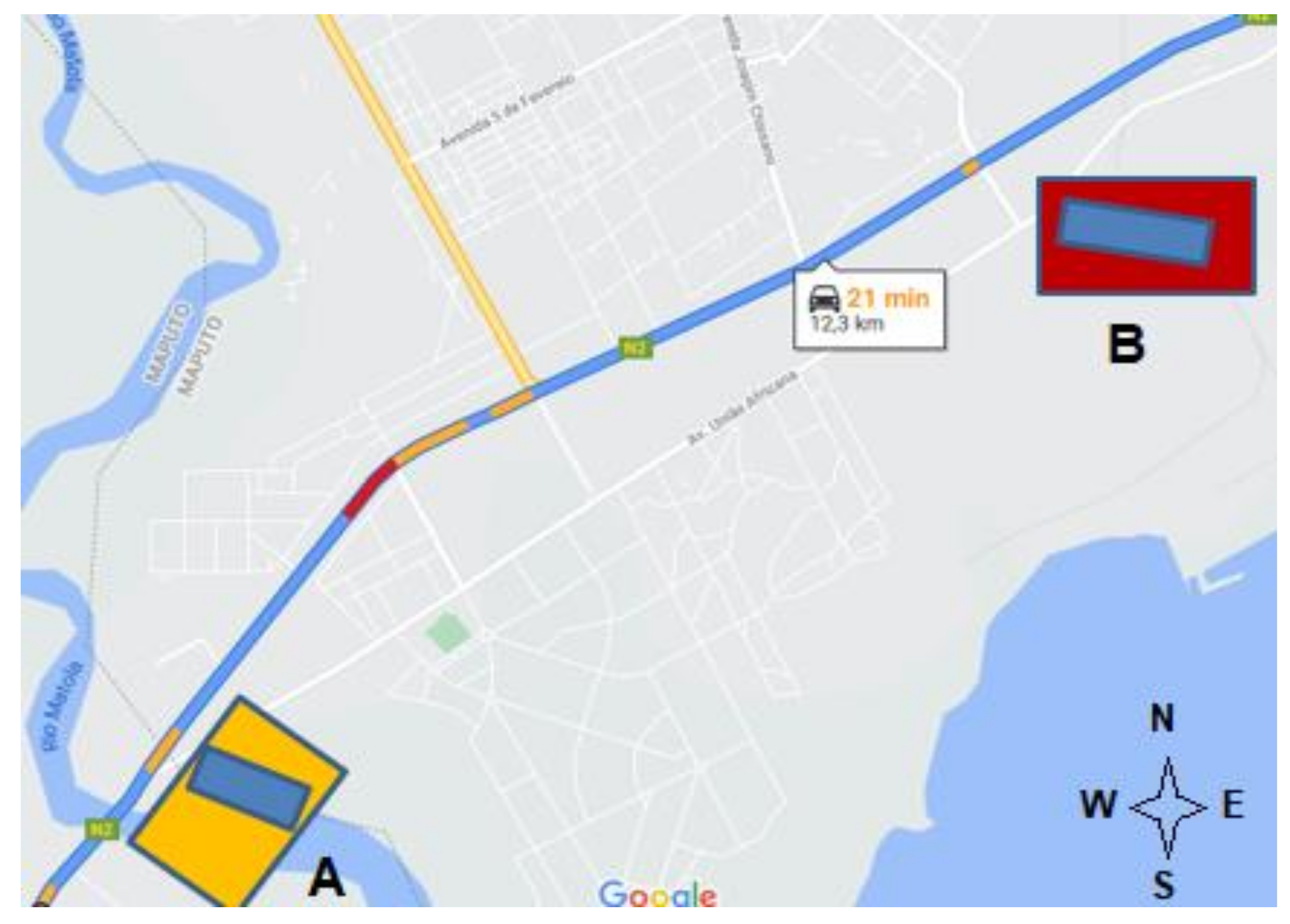
4. Case Study of Solar PV Systems in the Maputo Region
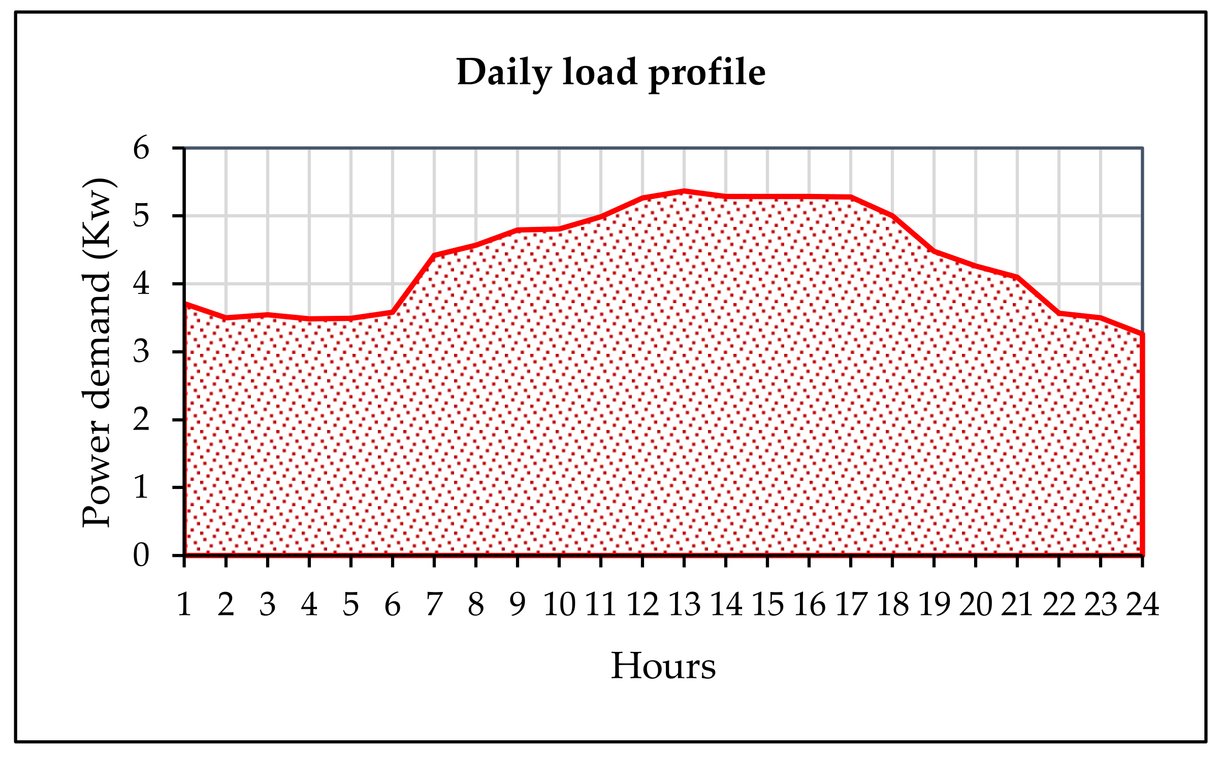
Considering the daily load profile, the availability of energy resources and investment costs, HOMER sized the capacity of the hybrid system composed by a 12.6 kW solar PV system, a 6.0 kW power storage bank, and a 6.0 kW DC/AC inverter.
- ▪
- The tilt and azimuth angle tracking method—evaluating the system’s power output for different tilt and azimuth angles, SAM provides four possibilities: fixed tilt and azimuth angles, rotation of the module on one of its axes, rotation of the module on one of its axes and its support, and finally the azimuth angle tracking option. In this study, the first option (fixed tilt and azimuth angles) was used as a basic case. As the methodology to track the optimal tilt angle, the azimuth angle was fixed equal to 0° and the tilt angle varied from 5 to 35° (Case-1). After optimizing the tilt angle, the azimuth varied from 0 to 30° to track the best angle (Case-1A).
- ▪
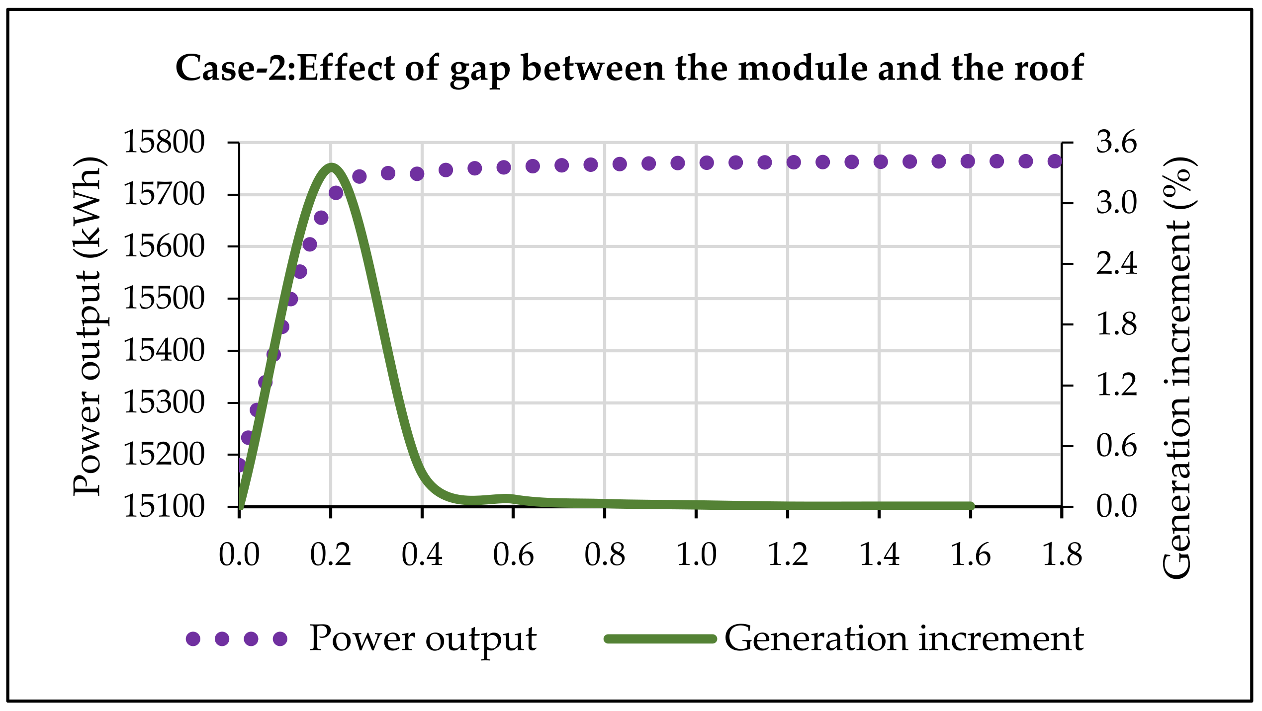
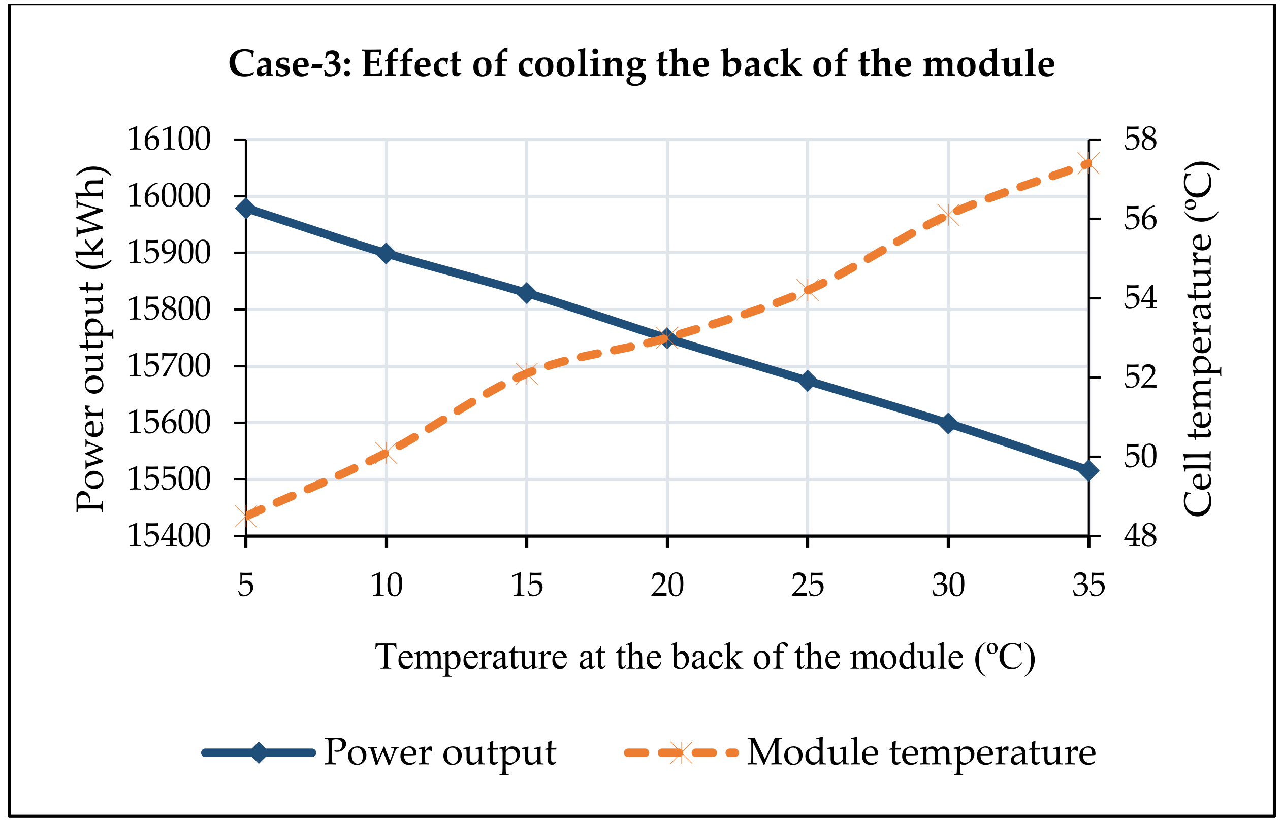
- Heat transfer method—examining the effect of ventilation at the back side of the module, in order to perform this analysis, SAM uses four mounting configuration options (rack, flush, integrated, and gap). In the rack configuration, the environment air flows freely over the front and back of the modules. In the flush configuration, the modules are in direct contact with the roof or wall and the environment air cannot flow over the back of the module. In the integrated mounting mode, the modules are part of the roof or wall and in the gap mounting mode, the modules are mounted to ensure a limited air flow over the backside of each module. In this study, the gap mounting mode (Case-2) and the integrated mounting mode (Case-3) were applied to assess thermal losses and module cell temperature. In Case-2 (the gap mounting mode), the space between the module’s back and the roof surface varied from 0 to 1.8 m in order to examine the effect of the natural flux of the air at the backside of the PV solar module. In Case-3, the integrated mounting mode was used to evaluate the effect of the module’s backside temperature.
5. Results and Discussion
6. Conclusions
Author Contributions
Funding
Institutional Review Board Statement
Informed Consent Statement
Data Availability Statement
Acknowledgments
Conflicts of Interest
References
- Gupta, P.; Kumar, B.; Wankhade, P.; Choudhary, P.; Singh, A.; Tiwari, A.K.; Singh, A.; Soni, A.; Shrivastana, N.; Bisen, N. Azimuth-Altitude Dual Axis Solar Tracker. IOSR J. Electr. Electron. Eng. 2016, 11, 26–30. [Google Scholar] [CrossRef]
- Stanislawski, B.; Margairaz, F.; Cal, R.; Calaf, M. Potential of module arrangements to enhance convective cooling in solar photovoltaic arrays. Renew. Energy 2020, 157, 851–858. [Google Scholar] [CrossRef]
- Keshavarz, S.A.; Talebizadeh, P.; Adalatia, S.M.; Mehrabian, A.; Abdolzadeh, M. Optimal slope-angles to determine maximum solar energy gain for solar collectors used in Iran. Int. J. Renew. Energy Res. 2012, 2, 665–673. [Google Scholar]
- Kumar, N.M.; Gupta, R.P.; Mathew, M.; Jayakumar, A.; Singh, N.K. Performance, energy loss, and degradation prediction of roof-integrated crystalline solar PV system installed in Northern India. Case Stud. Therm. Eng. 2019, 13, 100409. [Google Scholar] [CrossRef]
- He, G.; Kammen, D.M. Where, when and how much solar is available? A provincial-scale solar resource assessment for China. Renew. Energy 2016, 85, 74–82. [Google Scholar] [CrossRef] [Green Version]
- Darhmaoui, H.; Lahjouji, D. Latitude Based Model for Tilt Angle Optimization for Solar Collectors in the Mediterranean Region. Energy Procedia 2013, 42, 426–435. [Google Scholar] [CrossRef] [Green Version]
- Armstrong, S.; Hurley, W. A thermal model for photovoltaic panels under varying atmospheric conditions. Appl. Therm. Eng. 2010, 30, 1488–1495. [Google Scholar] [CrossRef]
- Chander, S.; Purohit, A.; Sharma, A.; Nehra, S.; Dhaka, M. Impact of temperature on performance of series and parallel connected mono-crystalline silicon solar cells. Energy Rep. 2015, 1, 175–180. [Google Scholar] [CrossRef] [Green Version]
- Gkaidatzis, P.A.; Bouhouras, A.S.; Sgouras, K.I.; Doukas, D.I.; Christoforidis, G.C.; Labridis, D.P. Efficient RES Penetration under Optimal Distributed Generation Placement Approach. Energies 2019, 12, 1250. [Google Scholar] [CrossRef] [Green Version]
- Udayakumar, M.; Anushree, G.; Sathyaraj, J.; Manjunathan, A. The impact of advanced technological developments on solar PV value chain. Mater. Today Proc. 2021, 45, 2053–2058. [Google Scholar] [CrossRef]
- Shen, L.; Li, Z.; Ma, T. Analysis of the power loss and quantification of the energy distribution in PV module. Appl. Energy 2020, 260, 114333. [Google Scholar] [CrossRef]
- Tan, L.; Date, A.; Fernandes, G.; Singh, B.; Ganguly, S. Efficiency Gains of Photovoltaic System Using Latent Heat Thermal Energy Storage. Energy Procedia 2017, 110, 83–88. [Google Scholar] [CrossRef]
- Tan, L.; Date, A.; Zhang, B.; Singh, B.; Ganguly, S. A Comparative Case Study of Remote Area Power Supply Systems Using Photovoltaic-battery vs Thermoelectric-battery Configuration. Energy Procedia 2017, 110, 89–94. [Google Scholar] [CrossRef]
- Khosravi, A.; Rodriguez, O.R.S.; Talebjedi, B.; Laukkanen, T.; Pabon, J.J.G.; Assad, M.E.H. New Correlations for Determination of Optimum Slope Angle of Solar Collectors. Energy Eng. 2020, 117, 249–265. [Google Scholar] [CrossRef]
- Jacobson, M.Z.; Jadhav, V. World estimates of PV optimal tilt angles and ratios of sunlight incident upon tilted and tracked PV panels relative to horizontal panels. Sol. Energy 2018, 169, 55–66. [Google Scholar] [CrossRef]
- Kuttybay, N.; Saymbetov, A.; Mekhilef, S.; Nurgaliyev, M.; Tukymbekov, D.; Dosymbetova, G.; Meiirkhanov, A.; Svanbayev, Y. Optimized Single-Axis Schedule Solar Tracker. Energies 2020, 13, 5226. [Google Scholar] [CrossRef]
- Jain, D.; Lalwani, M. A review on optimal inclination angles for solar arrays. Int. J. Renew. Energy Res. 2017, 7, 1053–1061. [Google Scholar]
- Goswami, D.Y. Principles of Solar Engineering, 3rd ed.; CRC Press: Boca Raton, FL, USA, 2015. [Google Scholar]
- Heide, D.; von Bremen, L.; Greiner, M.; Hoffmann, C.; Speckmann, M.; Bofinger, S. Seasonal optimal mix of wind and solar power in a future, highly renewable Europe. Renew. Energy 2010, 35, 2483–2489. [Google Scholar] [CrossRef]
- Muñoz, Y.; Orlando, V.; Gustavo, P.; Jairo, V. Sizing and Study of the Energy Production of a Grid-Tied Photovoltaic System Using PV syst Software. Tecciencia 2016, 12, 27–32. [Google Scholar] [CrossRef] [Green Version]
- Zappa, W.; Broek, M.V.D. Analysing the potential of integrating wind and solar power in Europe using spatial optimisation under various scenarios. Renew. Sustain. Energy Rev. 2018, 94, 1192–1216. [Google Scholar] [CrossRef]
- Liu, W.H.; Alwi, S.R.W.; Hashim, H.; Muis, Z.A.; Klemeš, J.J.; Rozali, N.E.M.; Lim, J.S.; Ho, W.S. Optimal Design and Sizing of Integrated Centralized and Decentralized Energy Systems. Energy Procedia 2017, 105, 3733–3740. [Google Scholar] [CrossRef]
- Soberanis, M.A.E.; Mithrush, T.; Bassam, A.; Mérida, W. A sensitivity analysis to determine technical and economic feasibility of energy storage systems implementation: A flow battery case study. Renew. Energy 2018, 115, 547–557. [Google Scholar] [CrossRef]
- Bhuvanesh, A.; Christa, S.J.; Kannan, S.; Pandiyan, M.K. Aiming towards pollution free future by high penetration of renewable energy sources in electricity generation expansion planning. Future 2018, 104, 25–36. [Google Scholar] [CrossRef]
- McLellan, B.; Florin, N.; Giurco, D.; Kishita, Y.; Itaoka, K.; Tezuka, T. Decentralised Energy Futures: The Changing Emissions Reduction Landscape. Procedia CIRP 2015, 29, 138–143. [Google Scholar] [CrossRef]
- Costa, T.S.; Villalva, M.G. Technical Evaluation of a PV-Diesel Hybrid System with Energy Storage: Case Study in the Tapajós-Arapiuns Extractive Reserve, Amazon, Brazil. Energies 2020, 13, 2969. [Google Scholar] [CrossRef]
- Branker, K.; Pathak, M.; Pearce, J. A review of solar photovoltaic levelized cost of electricity. Renew. Sustain. Energy Rev. 2011, 15, 4470–4482. [Google Scholar] [CrossRef] [Green Version]
- Popovici, C.G.; Hudişteanu, S.V.; Mateescu, T.D.; Cherecheş, N.-C. Efficiency Improvement of Photovoltaic Panels by Using Air Cooled Heat Sinks. Energy Procedia 2015, 85, 425–432. [Google Scholar] [CrossRef] [Green Version]
- Dubey, S.; Sarvaiya, J.N.; Seshadri, B. Temperature Dependent Photovoltaic (PV) Efficiency and Its Effect on PV Production in the World—A Review. Energy Procedia 2013, 33, 311–321. [Google Scholar] [CrossRef] [Green Version]
- Hammami, M.; Torretti, S.; Grimaccia, F.; Grandi, G. Thermal and Performance Analysis of a Photovoltaic Module with an Integrated Energy Storage System. Appl. Sci. 2017, 7, 1107. [Google Scholar] [CrossRef] [Green Version]
- Yang, H.; Wang, H.; Cao, D.; Sun, D.; Ju, X. Analysis of Power Loss for Crystalline Silicon Solar Module during the Course of Encapsulation. Int. J. Photoenergy 2015, 2015, 1–5. [Google Scholar] [CrossRef]
- Cengel, Y.A. Heat Transfer—A Pratical Approach, 2nd ed.; McGraw-Hill Inc.: New York, NY, USA, 2003. [Google Scholar]
- Tonui, J.; Tripanagnostopoulos, Y. Improved PV/T solar collectors with heat extraction by forced or natural air circulation. Renew. Energy 2007, 32, 623–637. [Google Scholar] [CrossRef]
- Saidan, M.; Albaali, G.; Alasis, E.; Kaldellis, J.K. Experimental study on the effect of dust deposition on solar photovoltaic panels in desert environment. Renew. Energy 2016, 92, 499–505. [Google Scholar] [CrossRef]
- Tao, S.; Li, C.; Zhang, L.; Tang, Y. Operational Risk Assessment of Grid-connected PV System Considering Weather Variability and Component Availability. Energy Procedia 2018, 145, 252–258. [Google Scholar] [CrossRef]
- Sharma, M.K.; Kumar, D.; Dhundhara, S.; Gaur, D.; Verma, Y.P. Optimal Tilt Angle Determination for PV Panels Using Real Time Data Acquisition. Glob. Chall. 2020, 4, 1900109. [Google Scholar] [CrossRef] [PubMed] [Green Version]
- National Renewable Energy Laboratory. System Advisor Model (SAM); NREL: Golden, CO, USA, 2020. [Google Scholar]
- FUNAE. Renewable Energy Atlas of Mozambique; Gesto Energia S.A.: Maputo, Mozambique, 2014. [Google Scholar]
- HOMER Energy. HOMER Pro. Available online: https://www.homerenergy.com/products/pro/index.html (accessed on 13 February 2021).
- EDM. Annual Statistical Report 2016; EDM: Maputo, Mozambique, 2016. [Google Scholar]
- Solar-panel-mounting-structure-2. Available online: https://grabcad.com/library/solar-panel-mounting-structure-2 (accessed on 12 May 2021).
- Benda, V.; Černá, L. PV cells and modules—State of the art, limits and trends. Heliyon 2020, 6, e05666. [Google Scholar] [CrossRef]
- Tuncel, B.; Ozden, T.; Balog, R.S.; Akinoglu, B.G. Dynamic thermal modelling of PV performance and effect of heat capacity on the module temperature. Case Stud. Therm. Eng. 2020, 22, 100754. [Google Scholar] [CrossRef]
- Hanifi, H.; Pander, M.; Zeller, U.; Ilse, K.; Dassler, D.; Mirza, M.; Bahattab, M.A.; Jaeckel, B.; Hagendorf, C.; Ebert, M.; et al. Loss analysis and optimization of PV module components and design to achieve higher energy yield and longer service life in desert regions. Appl. Energy 2020, 280, 116028. [Google Scholar] [CrossRef]
- Ameur, A.; Berrada, A.; Loudiyi, K.; Aggour, M. Forecast modeling and performance assessment of solar PV systems. J. Clean. Prod. 2020, 267, 122167. [Google Scholar] [CrossRef]
- Mulcué-Nieto, L.F.; Echeverry-Cardona, L.F.; Restrepo-Franco, A.M.; García-Gutiérrez, G.A.; Jiménez-García, F.N.; Mora-López, L. Energy performance assessment of monocrystalline and polycrystalline photovoltaic modules in the tropical mountain climate: The case for Manizales-Colombia. Energy Rep. 2020, 6, 2828–2835. [Google Scholar] [CrossRef]
- Chander, S.; Purohit, A.; Sharma, A.; Nehra, S.; Dhaka, M. A study on photovoltaic parameters of mono-crystalline silicon solar cell with cell temperature. Energy Rep. 2015, 1, 104–109. [Google Scholar] [CrossRef] [Green Version]
- Arab, A.H.; Taghezouit, B.; Abdeladim, K.; Semaoui, S.; Razagui, A.; Gherbi, A.; Boulahchiche, S.; Mahammed, I.H. Maximum power output performance modeling of solar photovoltaic modules. Energy Rep. 2020, 6, 680–686. [Google Scholar] [CrossRef]


| Module Structure and Mounting | (a) | (b) | dT (°C) |
|---|---|---|---|
| Glass/Cell/Polymer Sheet (open rack) | −3.56 | −0.075 | 3 |
| Glass/Cell/Glass (open rack) | −3.47 | −0.059 | 3 |
| Polymer/Thin Film/Steel (open rack) | −3.58 | −0.113 | 3 |
| Glass/Cell/Polymer Sheet (insulated back) | −2.81 | −0.045 | 0 |
| Glass/Cell/Glass (close roof mount) | −2.98 | −0.047 | 1 |
| Concentrating PV Module | −3.2 | −0.09 | 17 |
| Parameter | Value | |
|---|---|---|
| Nominal efficiency | 16.32 | % |
| Maximum power (pmp) | 420.01 | Wdc |
| Maximum power voltage (Vmp) | 49.50 | Vdc |
| Maximum power current (Imp) | 8.50 | Adc |
| Open circuit voltage (Voc) | 60.50 | Vdc |
| Short circuit current (Isc) | 9.00 | Adc |
| Parameter | Value | |
|---|---|---|
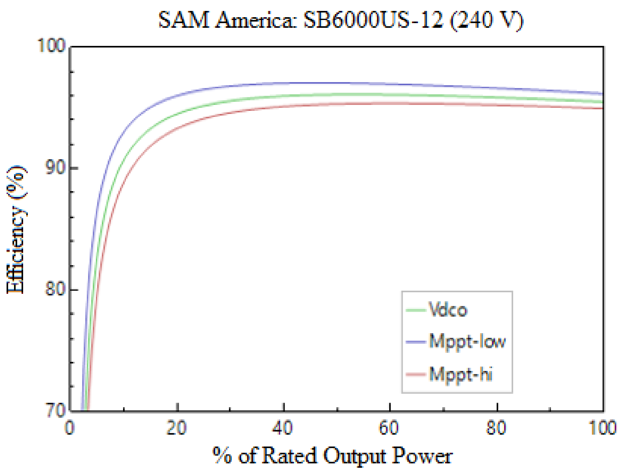
| Maximum AC power | 6000.00 | Wdc |
| Maximum DC power | 6282.08 | Wdc |
| Power use during operation | 51.58 | Wdc |
| Power use at night | 1.80 | Wdc |
| Nominal AC voltage | 240.00 | Vdc |
| Maximum DC voltage | 480.00 | Vdc |
| Maximum DC current | 20.25 | Adc |
| Minimum MPPT DC voltage | 100.00 | Vdc |
| Nominal DC voltage | 310.00 | Vdc |
| Maximum MPPT DC voltage | 480.00 | Vdc |
| Parameter | Value | |
|---|---|---|
| Nominal voltage | 39.60 | V |
| Nominal capacity | 53.00 | kWh |
| Nominal capacity | 256.00 | Ah |
| Roundtrip efficiency | 86.00 | % |
| Maximum charge current | 151.50 | A |
| Maximum discharge current | 151.50 | A |
| Metric | Value | |
|---|---|---|
| Annual energy (year 1) | 15,180.00 | kWh |
| Performance ratio (year 1) | 0.60 | |
| Battery roundtrip efficiency | 93.31 | % |
| Levelled COE | 15.40 | ¢/kWh |
| Net Actual cost | 28,696 | (USD) |
Publisher’s Note: MDPI stays neutral with regard to jurisdictional claims in published maps and institutional affiliations. |
© 2021 by the authors. Licensee MDPI, Basel, Switzerland. This article is an open access article distributed under the terms and conditions of the Creative Commons Attribution (CC BY) license (https://creativecommons.org/licenses/by/4.0/).
Share and Cite
Roque, P.M.J.; Chowdhury, S.P.D.; Huan, Z. Improvement of Stand-Alone Solar PV Systems in the Maputo Region by Adapting Necessary Parameters. Energies 2021, 14, 4357. https://doi.org/10.3390/en14144357
Roque PMJ, Chowdhury SPD, Huan Z. Improvement of Stand-Alone Solar PV Systems in the Maputo Region by Adapting Necessary Parameters. Energies. 2021; 14(14):4357. https://doi.org/10.3390/en14144357
Chicago/Turabian StyleRoque, Paxis Marques João, Shyama P. D. Chowdhury, and Zhongjie Huan. 2021. "Improvement of Stand-Alone Solar PV Systems in the Maputo Region by Adapting Necessary Parameters" Energies 14, no. 14: 4357. https://doi.org/10.3390/en14144357
APA StyleRoque, P. M. J., Chowdhury, S. P. D., & Huan, Z. (2021). Improvement of Stand-Alone Solar PV Systems in the Maputo Region by Adapting Necessary Parameters. Energies, 14(14), 4357. https://doi.org/10.3390/en14144357