Energy Dissipation during Surface Interaction of an Underactuated Robot for Planetary Exploration

Abstract

The article summarizes research on essential contributors to energy dissipation in an actuator for an exemplary planetary exploration hopping robot. It was demonstrated that contact dynamics could vary significantly depending on the surface type. As a result, regolith is a significant uncertainty factor to the control loop and plays a significant contribution in the control system development of future planetary exploration robots. The actual prototype of the actuating mechanism was tested on a reference surface and then compared with various surfaces (i.e., Syar, quartz sand, expanded clay, and quartz aggregate) to estimate the dissipation of the energy in the initial phase of hopping. Test outcomes are compared with multibody analysis. The research enhances trajectory planning and adaptive control of future hopping robots by determining three significant types of energy losses in the system and, most importantly, determining energy dissipation coefficients in contact with the various surfaces (i.e., from 4% to 53% depending on the surface type). The actual step-by-step methodology is proposed to analyze energy dissipation aspects for a limited number of runs, as it is a case for space systems.

1. Introduction

We present the research results into a high-energy and high-performance actuator developed for future scout hopping robots for planetary exploration applications. The overarching aspect of this research is to indicate the most critical energy components of the actuator’s work at its jump. Therefore, we focus on the phase of energy release in the actuator divided into three components: (1) energy dissipation resulting from the division of mass and inertia; (2) energy dissipation due to friction and losses in the mechanism; (3) energy dissipation resulting from regolith contact. The latter is essential because it allows reducing the uncertainties related to interaction with the regolith and adapt to variable surface conditions, which is one of the main risks when planning trajectories and controlling this type of robot. This article demonstrates the functionality of a 1-D prototype of an actuator applicable for space missions. Furthermore, it proposes the actual step-by-step methodology to analyze energy dissipation aspects for a limited number of runs as it is a case for space systems.

These results are particularly essential in the context of the recent intensification of surface exploration of the Moon and other bodies, as outlined by multiple frameworks, e.g., Lunar Exploration Roadmap, Strategy for Science at the Moon, Space Resources Strategy, or Artemis Science Definition Report. It is expected that multiple robotic and human-crewed missions will be launched in this decade to study Moon or asteroid resources, planetary processes, geological evolution, and other fundamental problems, many of which will require investigating rough and hardly accessible terrain of deep craters, lava tubes, steep slopes, and boulder fields.

Particular attention is also devoted to celestial bodies even smaller than the Moon (e.g., Near-Earth Objects, Phobos, Ceres, comets (e.g., [1]) where with reduced gravity, the traversability is more challenging, due to reduced weight and hence limited or almost not existing traction.

These goals and destinations arise from the need to extend in-situ planetary exploration beyond flat terrain, which offers limited possibilities for studying geological processes. However, a higher risk of mission failure characterizes such areas. Consequently, new methods are needed for more detailed terrain mapping and narrowing the uncertainty of terrain movement and trajectory planning. Additionally, awareness is raised towards expanding planetary infrastructure, demand for modular solutions, and shared knowledge to be used as building blocks for subsequent missions.

Those challenging needs are targeted by implementing more miniature robots and crafts assisting larger missions, mother landers, or rovers to increase their science return, overall mission safety, and diversification of tasks. The goal is also to ensure higher mission outcomes at a relatively lower cost than using a full-scale rover in a particular hard-to-reach area. Additionally, hard-to-access terrain can be investigated through other means of locomotion such as drones or helicopters, e.g., NASA’s Ingenuity (when an atmosphere is rich enough for such mobility). In contrast, subsurface and deep terrains can be investigated through robots like the Axel platform [2] with attached tethered ‘cliffhangers’ [3].

This article focuses on locomotion by hopping since it is one of the most widely considered scenarios of providing smaller scout capabilities as a part of a larger mission in lowered and micro-gravity. Only recently, hoppers were demonstrated to work on an extraterrestrial surface to explore the Ryugu asteroid by MINERVA-II rovers and the MASCOT lander. These robots had a tumbling-hopping capability and were the first use-case of mobile exploration on a small Solar System body [4]. We can also attribute such hopping ability to Rosetta’s Philae lander, although its hopping on 67P/Churyumov-Gerasimenko was unintended.

Multiple other platforms have previously been investigated for extraterrestrial use, including the PROP-F Phobos hopper [5], the NASA/JPL Hedgehog [6], a Comet Hopper [7], an elastic cage hopper [8], the Globetrotter airbag hopper [9], the Triton hopper [10], spherical robots [11], and our architecture, called Hopter [12]. Past research on hoppers includes, e.g., mechanisms design [13,14,15,16], testing [17], control [18,19,20,21,22,23] and optimization [24]. Bio-inspired design and control were also investigated in, e.g., [25,26] and references therein. Terrestrial test campaigns, e.g., [27], are rare due to the challenging recreation of relevant microgravity environments.

Hopping on soils and other granular materials was previously investigated to some degree thanks to biology and bionics, e.g., with human hopping [28], but also through hoppers research on compliant terrains [29,30,31,32,33]. The energy breakdown approach that we used to analyze dissipation was not used in previous works. Our method focuses on indexing the aggregated properties of the contact dynamics, which significantly simplifies predictions of the performance of the hopping system. The study described here applies to an actuator of a Hopter robot (Figure 1). However, the methodology and results are generalized and may apply to other space hopping systems. Specific contributions of the described research are:

• formulation of a valuable method for a limited number of runs and enabling the separation of crucial energy loss factors inside the highly energetic actuator;
• providing valuable data of energy dissipation during surface interaction as a critical factor for decreasing path planning uncertainties for planetary hopping robots;
• demonstration of the performance of the actual prototype of a highly energetic actuator suitable for utilization in a proposed hopping system for exemplary lunar scenarios.

2. Research Outline

2.1. Hopter—The Case Study

The case study for the research is the development of a Hopter hopping robot. The robot’s design is different from the previously mentioned, mainly due to three highly energetic actuating legs to repel the main body against the surface instead of internally actuated systems. The actuator’s principle of operation allows for achieving significantly higher efficiencies of the system. Hopter is designed for a lunar environment, convenient since once the problem is solved for that gravity, the design could be utilized in microgravity cases.

The objectives and overall architecture, applicability, and expected performance of Hopter were previously discussed in [34]. The actuation mechanism was also proposed in [35]. However, due to mass limitations, it has been redesigned and prototyped as described in this article. The scientific payload potentially applicable for Hopter was studied in [12].

This article addresses two significant problems in underactuated (e.g., hopping) robots for planetary exploration. The first one concerns the design of an actuator with an actuating leg, which allows for the accumulation of high energy (up to 50 J) at relatively low power consumption (below 5 W) and releases it instantly at the desired time. The second, consideration of methodology to monitor significant uncertainties of energy dissipation during surface interaction.

The architecture of Hopter is shown in Figure 1. For the current design, energy is accumulated in a set of springs, compressed using a DC motor through a ball screw system described in Section 2.2.1. The drive mechanism is placed behind each leg. The central location and one of the side compartments of the main platform are designated for control electronics, internal sensors, and batteries. The remaining two compartments are allocated for the scientific payload. The baseline mass allocation of the presented design can be outlined as follows (important for predictions of the performance later in the article):

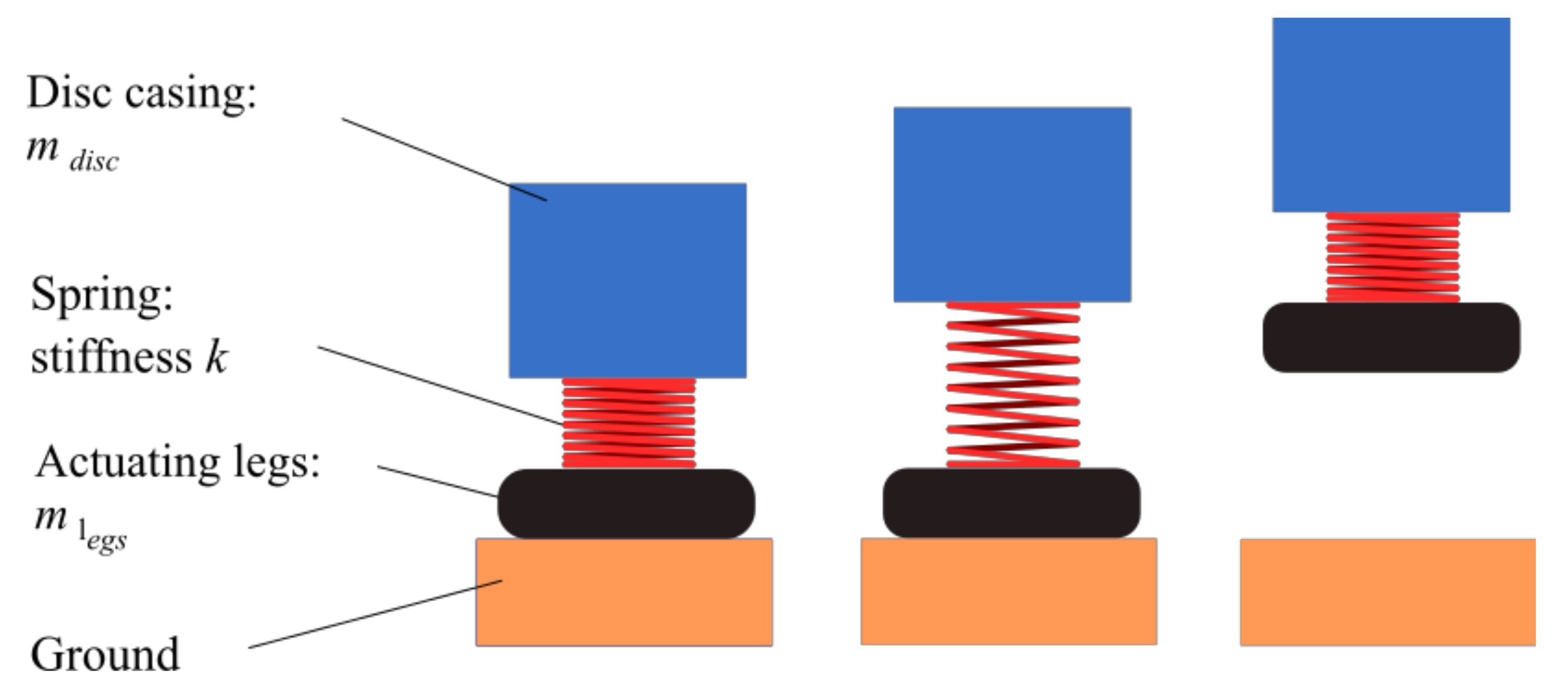
• main platform: 6.5 kg;
• actuating legs: 2.5 kg;
• drive springs: 1.0 kg (whilst the mass of the drive springs divides equally between the main platform and actuating legs).

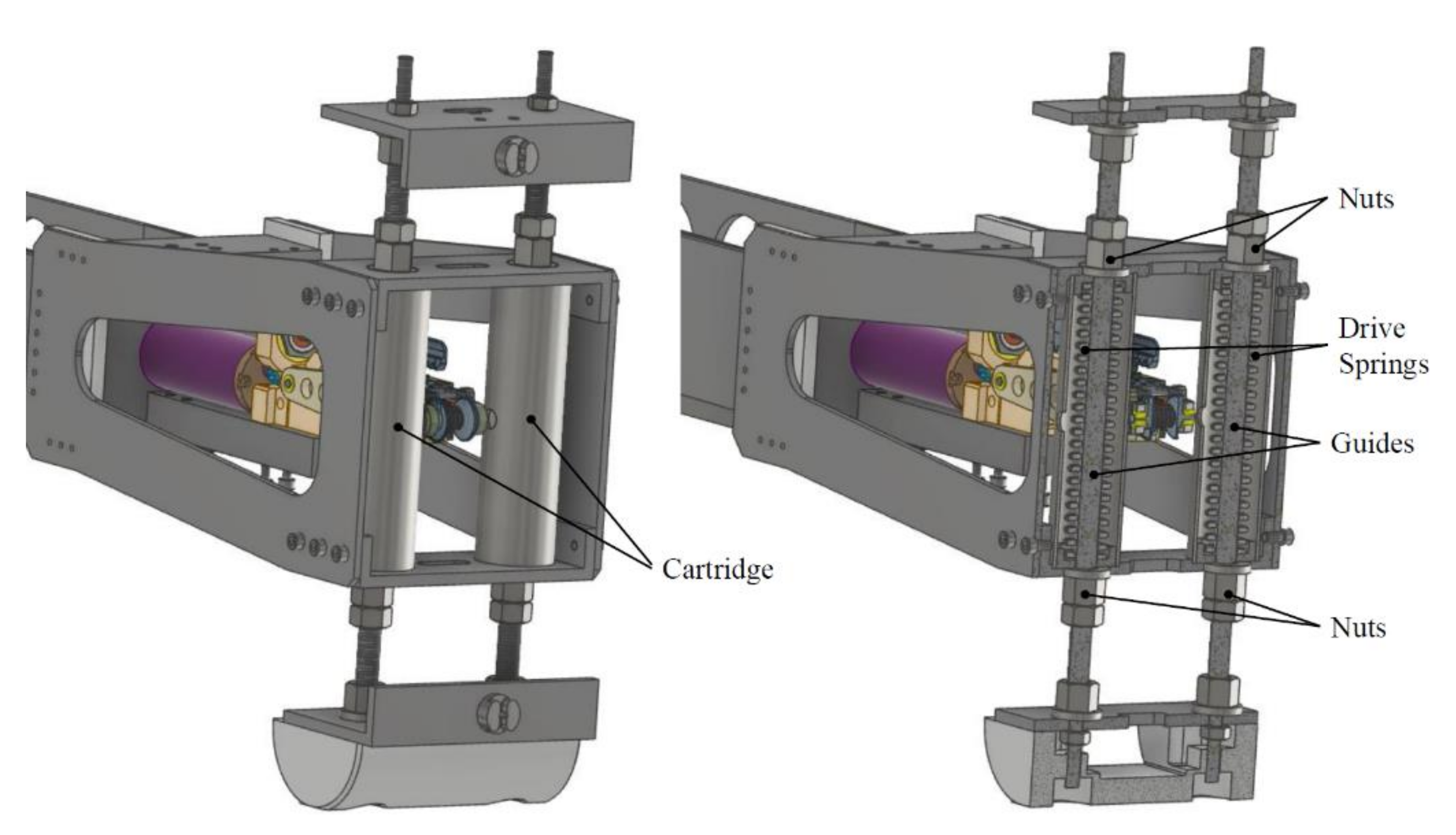
2.2. Design and Prototype of the Actuating Mechanism

The objectives and requirements of the actuator mechanism were previously described in [35]. Few models of the actuating mechanism have been developed. The prototyped one and described here is often referred here as BB-0B and consists of three main elements:

• An active system, called the actuator, aims to control loading the potential energy in the suspension and allow it to release at the desired moment. It is described in Section 2.2.1.;
• A passive system of accumulation and releasing mechanical energy called suspension, where energy is accumulated in two compression drive springs in a configuration introduced here as the floating spring design and described in Section 2.2.2.;
• The outer structure of the actuating leg which remains in contact with the surface and protects the interior of the robot (not studied in this research).

The actuating mechanism was tested on a 1-D testbed described in Section 3.4. It was mounted to a rotating arm typical only for the testbed to constrain the operation to one plane only (for instance, shown in Section 2.2.2.).

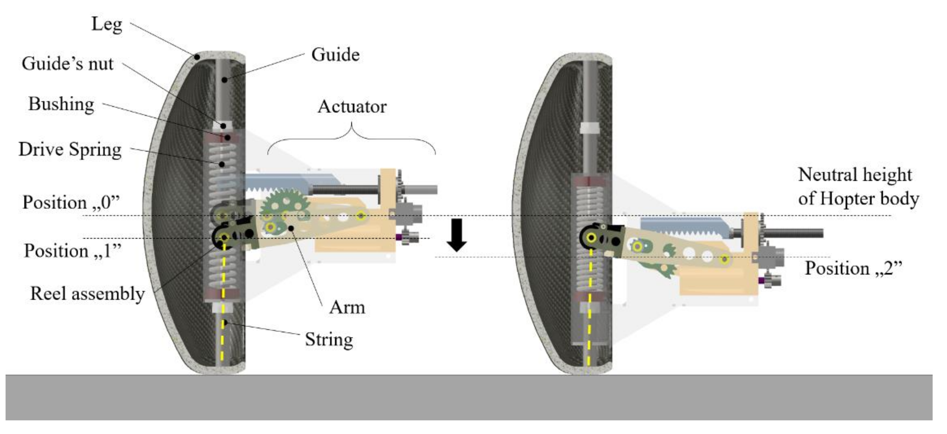
2.2.1. The Operational Sequence of the Actuator

The principle of operation and main components of the actuating mechanism are shown in Figure 2 (as designed in baseline configuration) and Figure 3 (the actual hardware for the tests conducted in this research). The sequence of energy accumulation and release consist of three phases:

• The arm is actuated through a gear and a ball screw. It is relocated from neutral (horizontal) position “0” downwards to the extreme position “1”. The string is locked in the reel assembly;
• The arm is moved upwards and pulls the leg against the drive springs through the string. Naturally, the legs rest on the ground; therefore, the main platform is being lowered to position “2”;
• Position “2” can be adjusted to tension the drive springs to the desired energy levels. Once it is reached, the reel assembly is ready to release the string, the main platform is accelerated upwards, and performs the jump.

2.2.2. Actuating Leg Suspension with Drive Springs

The main requirement for this design was to minimize the mass of the components, therefore, to use the same set of springs to accumulate energy regardless of jump direction. We introduced a concept of a floating spring, as shown in the schematic sequence of operation in Figure 4. The detailed design and actual model mounted on the rotating arm are shown in Figure 5 and Figure 6.

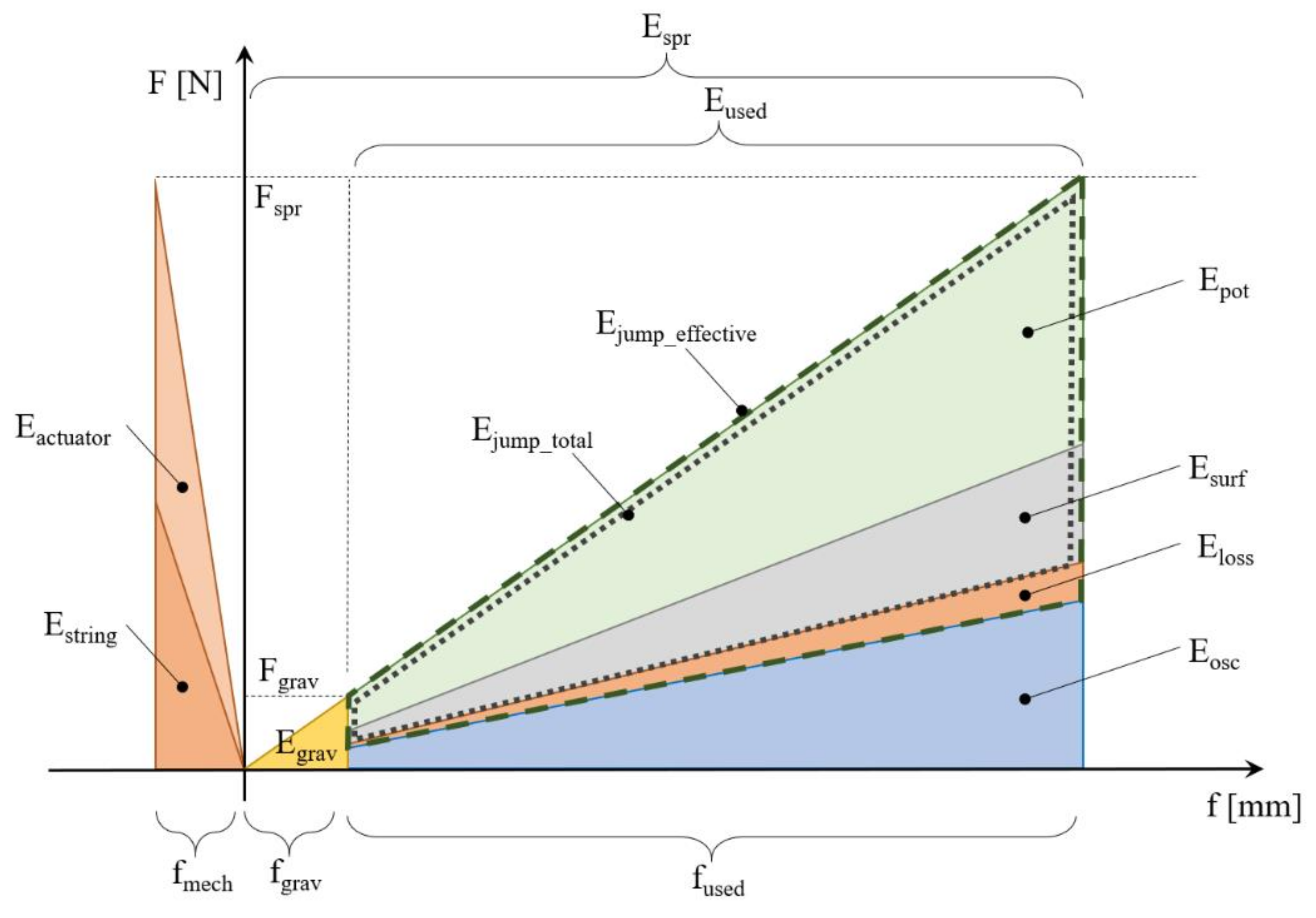
2.2.3. Definition of Energies Occurring in the Actuating Mechanism and Jumping Process

The research was limited only to the event of the initiation of the jump (i.e., not landing). The energy components contributing to the energy accumulation process were identified accordingly in this section. Ultimately, this is needed to isolate the direct jump energy and estimate energy dissipation during surface interaction. The problem can be considered from the perspective of forces, deflections, and resulting stiffnesses in the mechanism. During the test campaign, besides the drive springs elastic deformation, the actuator and the strings that pull the actuating leg have large and non-negligible stiffnesses. The potential energy accumulated on the side of the actuator does not influence the jump directly. Still, it lowers the effective as-designed compression of the drive springs (an important lesson learned when designing high-force and high-energy actuators for hopping robots).

The mechanism’s different deflections and forces are defined and shown in the schematic plot in Figure 7. As shown in this figure, the drive springs react with force F_spr when compressed to distance f_grav + f_used, which at the same time causes the deflection f_mech of the actuator and the string, which transfers the force between the actuator and the actuating leg (with the drive springs compressed between them). Therefore, on the left side of the plot are the deflections of the string and the actuator. Naturally, the area of the field is interpreted as energy. Once the electromagnet is triggered and the lock arm opened, the string no longer transfers forces. Therefore, energies between the left and right sides of the plot are utilized independently. The definitions of identified energies from Figure 7 are listed in

Table 1. Description of the energy contributors.

Symbol	Description	Expected Value at Baseline in Hopter (the Full-Scale Target Model)	Contribution to the Jump
The right side of the plot
Espr	Total potential energy accumulated in the drive springs	Greater than 50 J to compensate for surface interaction losses, other contributors, and the left-hand side factors	Yes, directly
Egrav	Initial potential energy accumulated in the springs resulted from the weight of the hopper resting on the springs.	Becomes insignificant for larger stiffnesses of the drive springs and smaller gravities. Expected <1% of the Espr	Not contributing to the jump directly but reduces the effective Espr to Eused
Eosc	The energy lost in the momentum exchange between disc casing and actuating legs	It depends on the mass ratios, as demonstrated in Section 3.2. Expected between 20–40% of the Espr	Yes, it reduces the Ejump_total
Eloss	All losses linked to the dynamics of the actuating mechanism during the release of the springs, e.g., the kinetic energy of the reel axis (Ereel kinetic), internal and external friction of the drive springs (Esus) or any other undefined, e.g., atmosphere drag (Eother)	Expected to reduce below 5% of the Espr	Yes, it reduces the Ejump_effective
Esurf	The energy dissipated in the contact of the leg with the surface (regolith, soil, etc.)	Depends on the surface material and design of the foot of the actuating leg	Yes, it reduces the Epot
Epot	The remaining effective kinetic/potential energy resulting from the jump	In the laboratory conditions can be measured either by the height of the jump (hmax) or the maximum velocity of the robot. The objective is to maximize this energy	Pure jump energy
The left side of the plot
Estring	Potential energy accumulated in the elongation of the string	Ideally should be minimized by proper design	Not contributing to the jump. Only reducing effective compression of springs
Eactuator	Potential energy accumulated in the elastic deformation of the actuator when acting against the drive springs through the string

.

3. Materials and Methods

3.1. Objectives and Basic Methodology Description

The surface interaction uncertainties can be tackled by two methods: system force analysis or system energy analysis. The force analysis would require additional force gauges in actuating legs for direct measurements of the reaction forces. It most likely would increase the complexity of space robotic systems, which should tend for simplifications by design. The energy approach bypassed the contact forces but is simpler for implementation to planetary exploration robots. It focuses on the effects of a jump and utilizes the internal sensors that are already on board the robot. In this research, we have chosen the energy approach, and consequently, the main objectives of the test can be outlined:

• demonstrate the system’s functionality on the actual prototype, i.e., symmetrical actuation of the floating spring, actuating mechanism tensioning the actuating leg through a reel assembly and string system;
• validate the multibody analysis and confirm the assumed dynamics of the system;
• identify the percent of energy dissipated or lost in the actuating mechanism;
• identify the percent of energy dissipation in contact with the surface to narrow down the hopping uncertainties;
• eventually, demonstrate how the method translates to errors of the performance predictions of the 1-D system utilizing the identified coefficients as simple scaling factors in the control loop.

The methodology used to demonstrate those objectives was to conduct a series of tests with a prototype of an actuating mechanism and then compare it with the results obtained in a numerical model simulated in MSC Adams software.

The validation of the numerical model using MSC Adams software is done by comparing the simplified analytical model presented in the following section. Then, the tests on solid surfaces were used to capture the reference jumps where we assume the energy surface dissipation is negligible. By comparing it with the theoretical performance from numerical simulation, we can obtain the mechanical losses in the system. Once the repeatability of those was confirmed, the tests with regolith analogs were performed. Consequently, the delta energy between the reference tests and tests with regolith analogs is considered the regolith’s dissipated energy.

In this methodology, the following constraints were considered:

• the tests are done in Earth gravity only. Extrapolating the results to other gravities was not a subject of this work. Advanced methods are considered, e.g., [36,37];
• the energy losses due to atmospheric drag are considered negligible. They are part of loss energy E_loss as defined in Table 1 and are not concerned at this level of detail in this research;
• the tests are unidirectional, and the primary focus is on dissipation energy normal to the surface since they become a point of reference to other configurations which may be considered in the future. One set of tests was done for a configuration inclined by 20°, which is helpful to indicate the amount of energy dissipation when lateral forces occur in the vectorization of a 3-D system;
• the energy dissipation of surface interaction is a property of a pair of objects (i.e., surface material and actuating leg); therefore, various shapes and contact areas are studied.

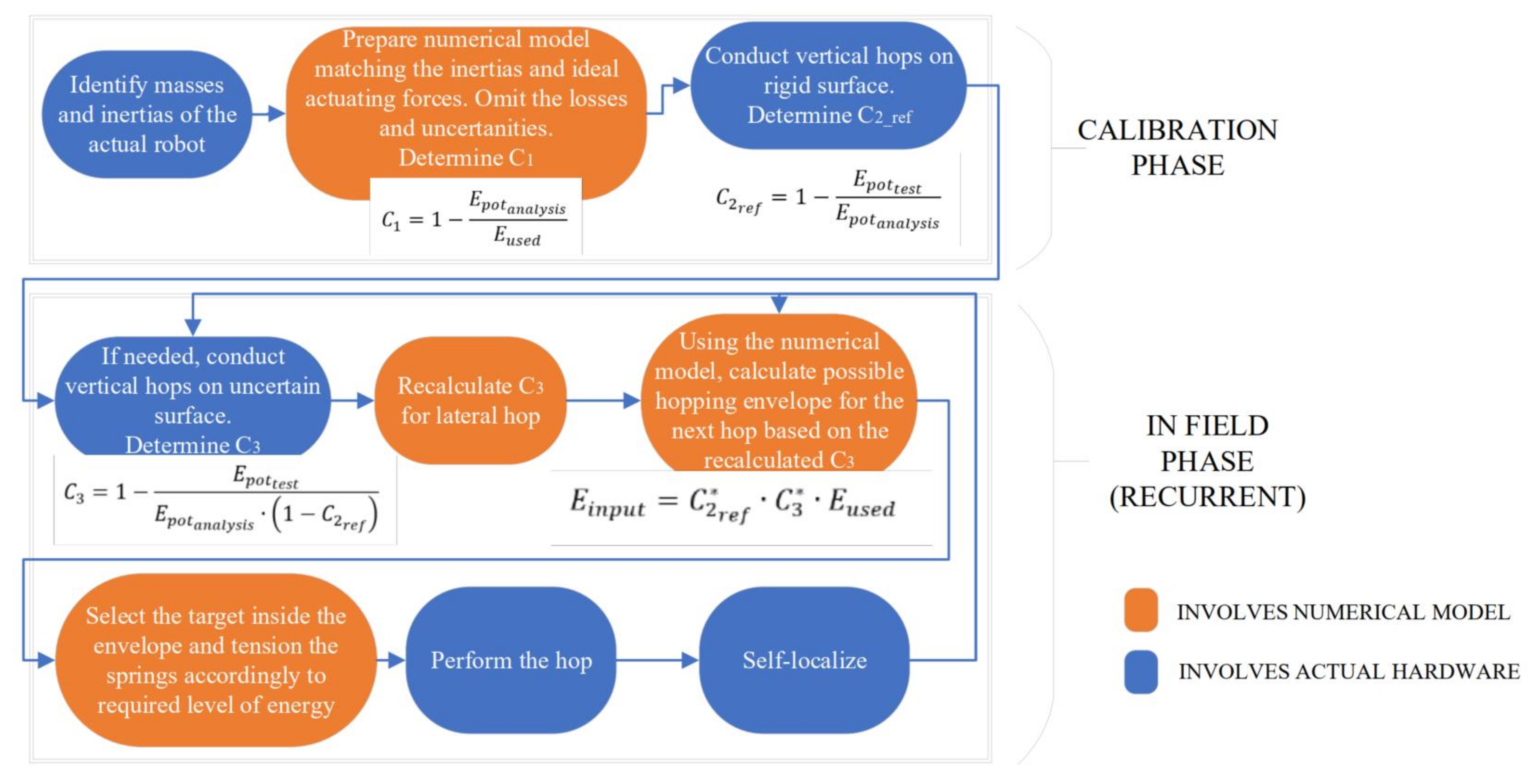
3.2. Cross-Validation of the Reference Models. Definition of Factor C₁

The methodology we propose utilizes a multibody model used to reference the performance of the actual hardware. An additional analytical model is needed to validate the multibody analysis. We consider a two-mass system that hops vertically (Figure 8). It shall match with the performance of the reference jumps of the test device and the multibody analysis of the testbed and 3-D system jumping vertically—the description of this 1-D analytical model is in Appendix A. The general outcome of the model’s validation is shown in Figure 9. As seen from the plot, there is a satisfactory correlation between the simplified analytical model, the full-scale 3-D numerical model (in the configuration shown in Figure 1), and the actual 1-D numerical model of BB-0B, proving that models are validated and can be utilized with the proposed methodology. The actual jump energy (E_{jump_total}) is directly proportional to the ratio of the masses of the system, and the accumulated energy in the springs E_spr (initial compression of the springs under the weight of the m_disc is neglected for this simplified model, see Appendix A).

Consequently, there is always an energy loss associated with the momentum exchange in the hopping system unless the actuating leg is mass-less. It manifests in residual oscillations of the drive springs. We can therefore introduce a proportional jumping efficiency factor $C_1^{*}$ that can be analytically determined (see Equation (1), where M = m_disc + m_legs as defined in Appendix A). Here we are considering the linear motion, and therefore pure masses are taken. For complex or rotational movements, the moments of inertias should be considered.

$$E_{jum{p}_{total}}=E_{spr}·\frac{m_{disc}}{M}=C_1^{*}·E_{spr}=\left(1-C_1\right)·E_{spr}$$

(1)

3.3. The Theoretical Model of the Energy Losses in the System (Definition of Energy Loss Coefficients)

The energy components monitored during the tests and in the analysis are shown in detail in Figure 7. They are represented in a nested manner, which helps to understand the flow down of the energy components. The drive springs are compressed to spring energy (E_spr); under gravity, there is always an initial compression of the drive springs attributed to the weight of the mechanism, which is shown as E_grav. As a result, the energy that contributes to the energy exchange between masses is referred to here as E_used, a subtract product of E_spr and E_grav. From Section 3.2, we know that a portion of the energy (E_osc) is lost in momentum exchange between the hopping masses. In actual performance, those residual oscillations of the drive springs will tend to damp. The remaining energy we define here is total jump energy (E_{jump_total})_. Out of this energy, we naturally assume that due to the friction in the sliding parts of the mechanism, a portion of the energy will be lost (E_loss). Finally, the remaining amount of the energy is the effective jump energy E_{jump_effective}, which can be divided between the energy that is the pure kinetic energy of the mechanism and energy dissipated in the surface (E_surf). For the vertical hops, which we consider in this article, the kinetic energy can also be measured as potential energy (E_pot), when the mechanism reaches the maximum height of the jump (h_max).

As derived in Appendix B the relation between E_spr and E_pot depends on the three following factors:

• Coefficient of energy loss in the momentum exchange (C₁, also $C_1=1-C_1^{*}$);
• Coefficient of energy loss in the mechanism’s friction (C_{2_ref}, also $C_2=1-C_2^{*}$) It will come in handy later that C_{2_ref} can be calculated against all trials (multiple runs) or for specific reference jumps done before jumping on non-solid surfaces. Therefore, we get: C_{2_ref_avarage} or C_{2_ref_direct}. Ideally, C_{2_ref_avarage} and C_{2_ref_direct} should be the same or close to each other, which would prove that the results of this approach are consistent;
• Coefficient of energy dissipation in the surface (C₃, also $C_3=1-C_3^{*}$).

As shown in Appendix B, the coefficients can be calculated by comparing the potential energies of the actual system with the one from the loss-free numerical model:

$$C_1=1-\frac{E_{po{t}_{analysis}}}{E_{used}}$$

(2)

$$C_{2_{ref}}=1-\frac{E_{po{t}_{test}}}{E_{po{t}_{analysis}}}$$

(3)

$$C_3=1-\frac{E_{po{t}_{test}}}{E_{po{t}_{analysis}}·\left(1-C_{2_{ref}}\right)}$$

(4)

Using those coefficients, we can define the general relation between the potential energy of the system (and hence the maximum height of jump h_max) in the given gravity (g):

$$\begin{gathered} E_{pot}=\left(1-C_1\right)\left(1-C_{2_{ref}}\right)\left(1-C_3\right)\left(E_{spr}-E_{grav}\right) \\ =C_1^{*}·C_{2_{ref}}^{*}·C_3^{*}·\left(E_{spr}-E_{grav}\right) \end{gathered}$$

(5)

$$h_{max}=\frac{E_{pot}}{Mg}=\frac{C_1^{*}·C_{2_{ref}}^{*}·C_3^{*}·\left(E_{spr}-E_{grav}\right)}{Mg}$$

(6)

Relations (5) and (6) help understand how to maximize the metrics (e.g., height of jumps) of a hopping robot by maximizing those factors (assuming E_spr is already defined and maximized):

• $C_1^{*}$ can be maximized based on the analysis done in Figure 9;
• $C_2^{*}$ depends on the friction and design of the mechanism itself;
• $C_3^{*}$ depends on two factors: (1) properties of the surface which we can only control by navigating the robot through surfaces characterized by a high $C_3^{*}$ coefficient or (2) hypothetically by a design of the actuating leg (e.g., by increasing its surface-to-surface contact, which needs to be confirmed by tests).

Eventually, the model shall be used in reverse analysis and actual control loop to feedback the measured C₂ and C₃ to the input energy of the numerical analysis and calculate the expected performance of the actual system without implementing complex contact dynamics with the ground. This approach greatly simplifies the numerical models and allows for the utilization of simple coefficients for trajectory planning on unknown surfaces, and does not require other sensors than those already existing on the robot. The robot’s on-board processing could also be simplified. Essentially, the input energy feedbacked to the numerical model will be (7). The response of the numerical model (height of a jump $h_{analysis}$) is later compared to the actual system response ($h_{test}$). The mean absolute error (MAE) can be calculated.

$$E_{input}=C_{2_{ref}}^{*}·C_3^{*}·E_{used}$$

(7)

Following the theoretical considerations from above, during the test, we monitored the corresponding parameters and variables:

• mass distribution of the components of the testbed and its configuration was recorded to match coefficient C₁ properly;
• measured and recorded compression of the springs from actuating mechanism for each test run. The distances were measured with a caliper, directly before the tensioning and then just before the jump; the calculated delta is dimension f_used in Figure 7;
• initial compression of the springs from the weight of the system was calculated from a given stiffness constant and measured mass (M) of the device under test (distance f_grav in Figure 7);
• with the above measurements, total accumulated energy in the springs was established (E_spr), their force (proper to determine load limits of the mechanism), and eventually the energy devoted to jump itself (E_used);
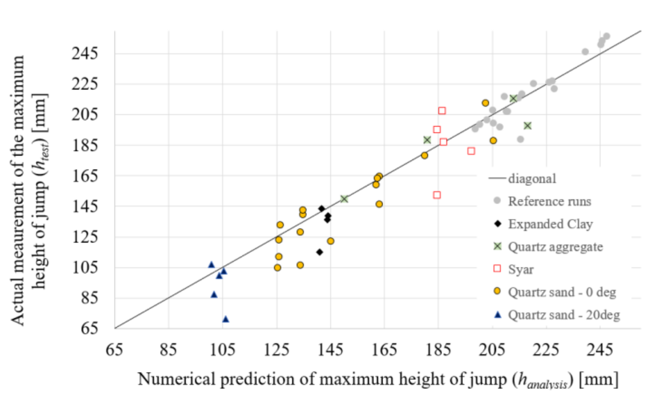
• height of jump of the center of mass in the numerical model ($h_{analysis})$ and actual tests-bed ($h_{test}$) were monitored;
• the other parameters and coefficients are linked to Equations (2)–(4) and outlined in Appendix B.

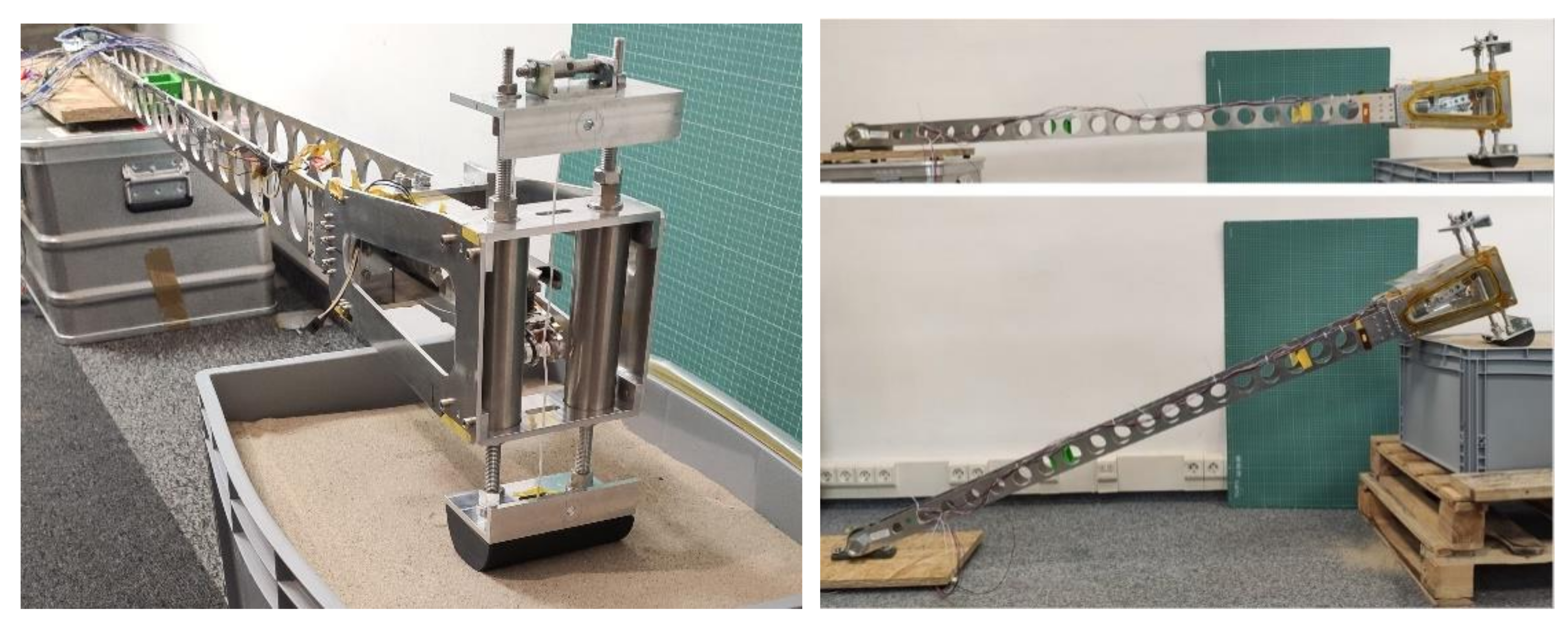
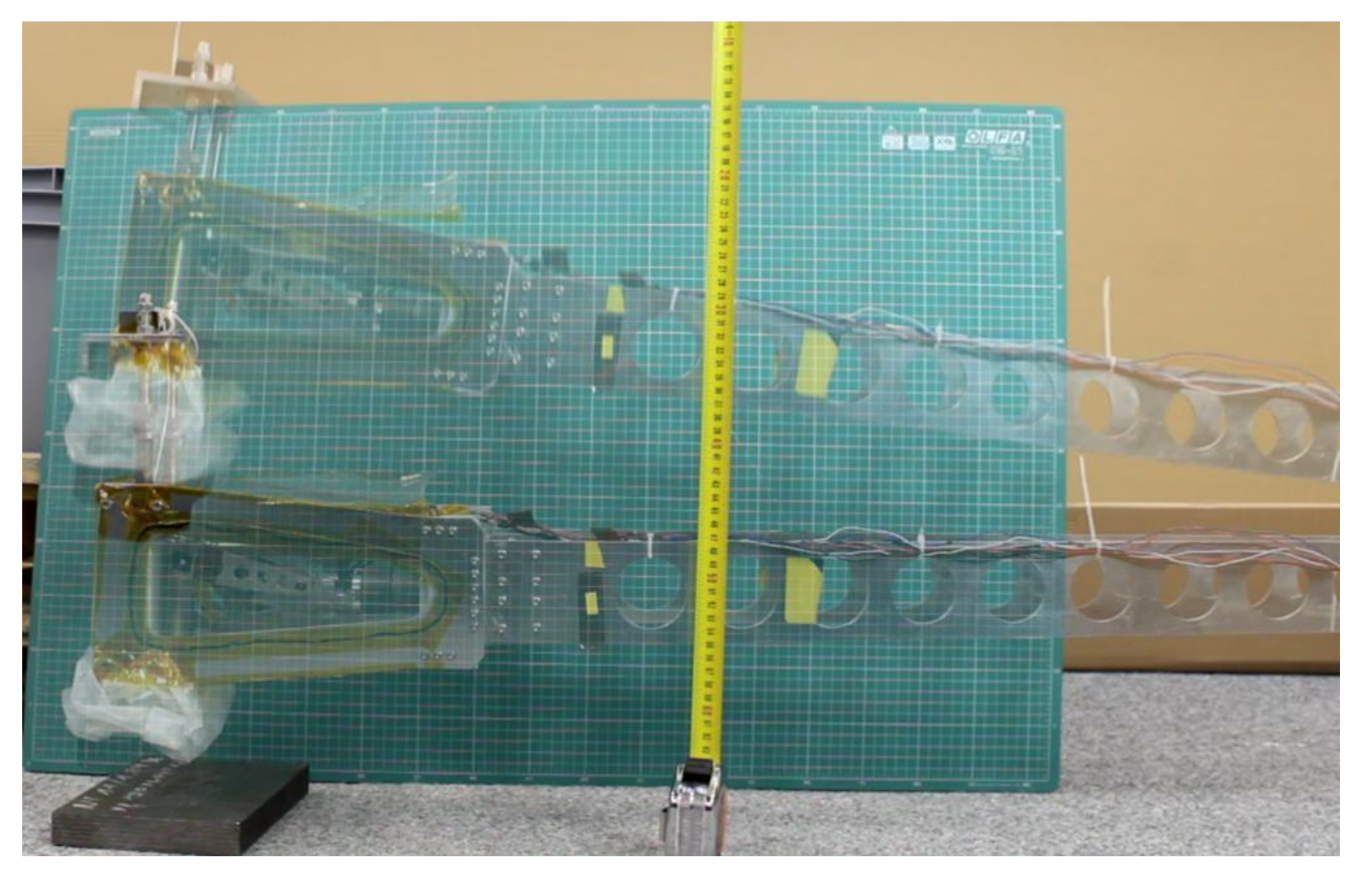
3.4. Description of the BB-0B Test Set-Up and Test Plan

The full-scale model of Hopter possesses 9 degrees of freedom (three for the actuating legs, 3 translational, and 3 rotational). For the BB-0B device, most of the degrees of freedom were isolated. Only two were left (one for the actuating leg and another to constrain the movement in one plane) to directly measure the hopping energy by measuring the height of a jump. An actuating mechanism mounted on the arm with a hinge (i.e., rotational movement) was selected as the testbed configuration (Figure 6).

The typical test scene is shown in Figure 10. It consists of the actuating mechanism mounted with a long rotational arm, optional background, lights and cameras: standard camera and occasionally high-speed camera. The actuating mechanism was powered via a laboratory power supply. The release of energy (performed with actuation of the electromagnet and lock arm) was done by a Raspberry Pi computer, which controlled the PWM of the electromagnet and time of actuation. The typical recorded scene was analyzed in a post-process, as shown in Figure 11.

The test procedure was executed each time in the following sequence:

• Prepare the surface;
• Make sure the mechanism is aligned and free to move;
• Measure the initial distance between the foot and the body (initial state of the compression);
• Compress the springs to the desired energy (here in BB-0B, we always used the maximum compression, which allowed them to accumulate up to 24 J);
• Measure the final distance between the foot and the body and calculate the delta f_used;
• Turn on a camera placed perpendicular to the actuation plane and point towards the center of mass (CoM) of the test set-up;
• Trigger the electromagnet to disarm the holding mechanism;
• The jump is performed;
• Stop recording and turn off the power supply after the movement is settled back.

A barefoot configuration (the reference) was tested, and four other types of footpads were assembled on the actuating legs. They differ in terms of contact area with the surface and their inertias:

• Configuration #0—actuating leg with a barefoot configuration where two steel rods finished with small, rounded nuts are in direct contact with a hard metallic surface. The steel-on-steel pair was chosen to ensure high rigidity between the surface and the actuating leg. Consequently, this one was used in the initial reference jumps to compare the analytical model since the energy dissipation on the rigid surface can be considered negligible.
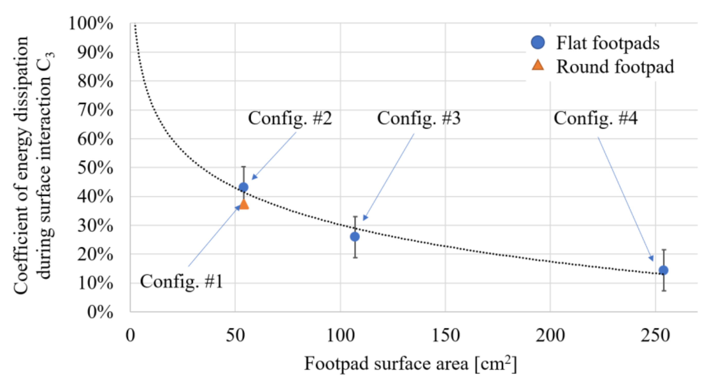
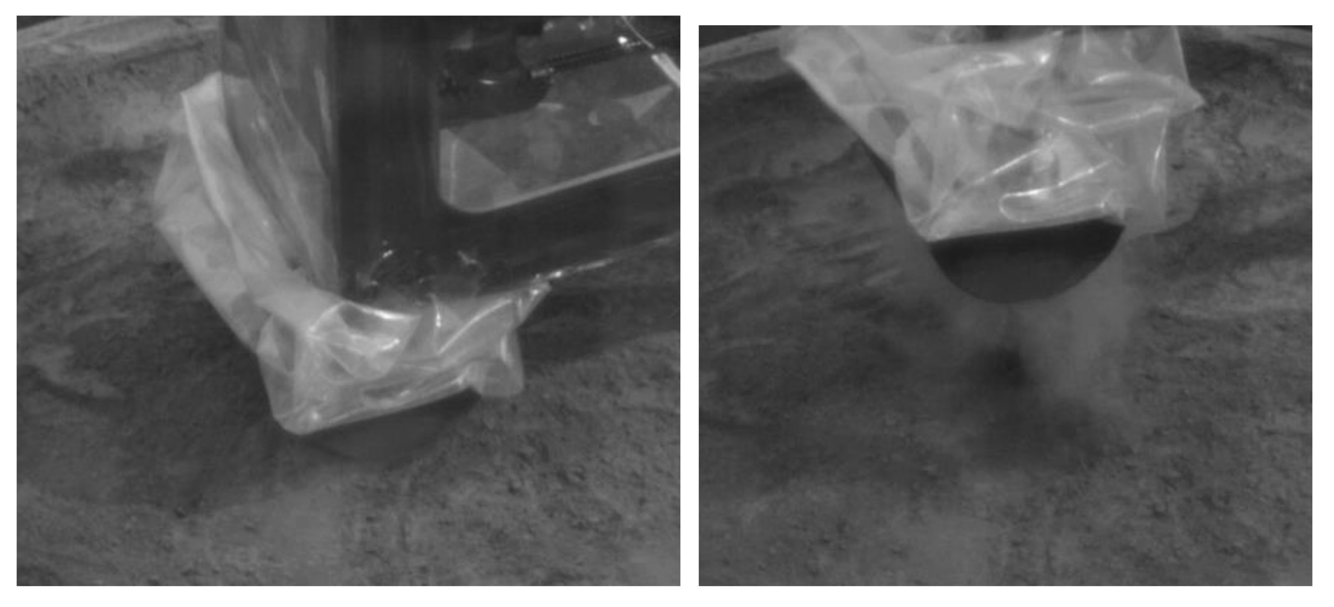
• Configuration #1—actuating leg with a rounded foot in the shape of a half-cylinder 134 mm long and with a radius of 40 mm. The effective contact area with quartz sand was measured to around 54 cm².
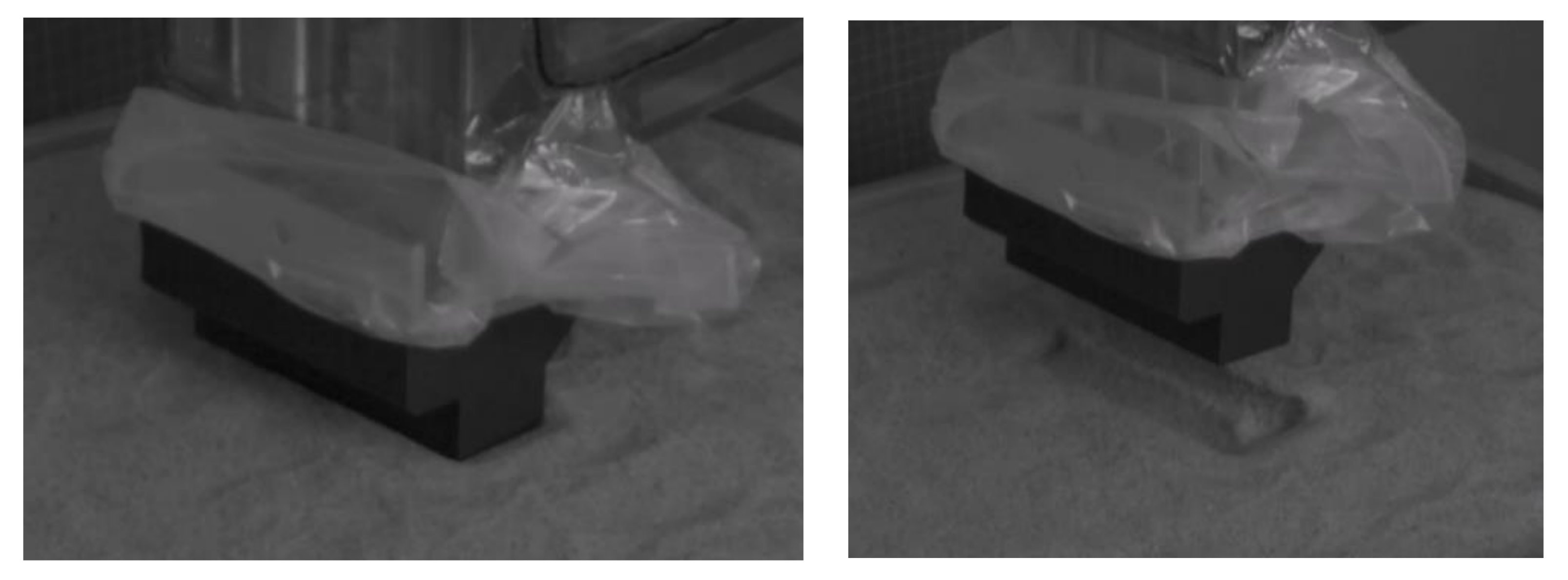
• Configuration #2—actuating leg contact area like in configuration #1 (around 54 cm²), but with a flat footpad instead.
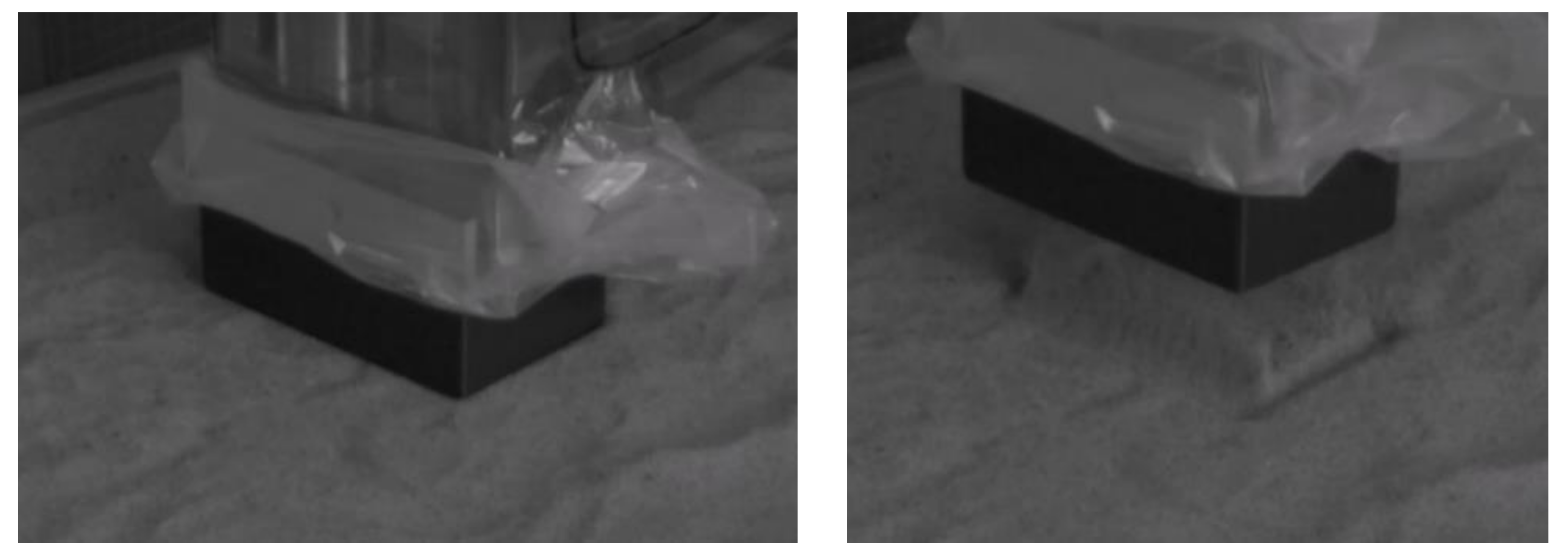
• Configuration #3—actuating leg with a flat surface contact area based on a width equivalent to the diameter of the round foot from configuration #1 (around 107 cm²).
• Configuration #4—actuating leg with a flat foot with a contact area significantly larger (here 4.8 times) than contact area from configuration #1 (around 257 cm²).

The shapes of feet were chosen to maximize the expected outcome of the tests under limited trials:

• Feet with flat surface contact areas (#2, #3, #4) were used to provide information on the scaling laws of dissipation coefficient against the contact areas;
• Round foot (#1) can be compared with small and medium feet (#2, #3), from which observations can be derived on drag coefficients depending on the shape of the foot;
• Round foot possesses the same contact with a surface regardless of the angle of actuation and therefore is used as a reference foot for comparison of performance between all types of regolith analogs and at tilted test.

Those foot configurations are shown in Figure 12 and Figure 13. The mass and inertias of those configurations are provided in Section 3.5. All feet are 3D-printed with the same printer settings and made of ABS material from the same producer.

Except for the rigid surface (steel plate), which was treated as the reference surface, the tests were conducted on four analog surfaces shown in Figure 14 and

Table 2. Characteristics of the surface materials used in the tests.

Type of Material	Description	Average Density [kg/m3]
Syar	Analogue of Martian regolith, highly cohesive	2010
Quartz sand	Grain size: 0.5–1.0 mm	1840
Expanded clay	Grain size: 8–16 mm	270
Quartz aggregate	Grain size: 8–16 mm	1700

. We selected a relatively large box container for the materials (shown partially in Figure 6) to minimize the influence of the presence of the walls on the boundary conditions (dimensions 37 cm by 56.4 cm and soil depth 25.4 cm). The material selection was made to maximize the differences between the compared surfaces:

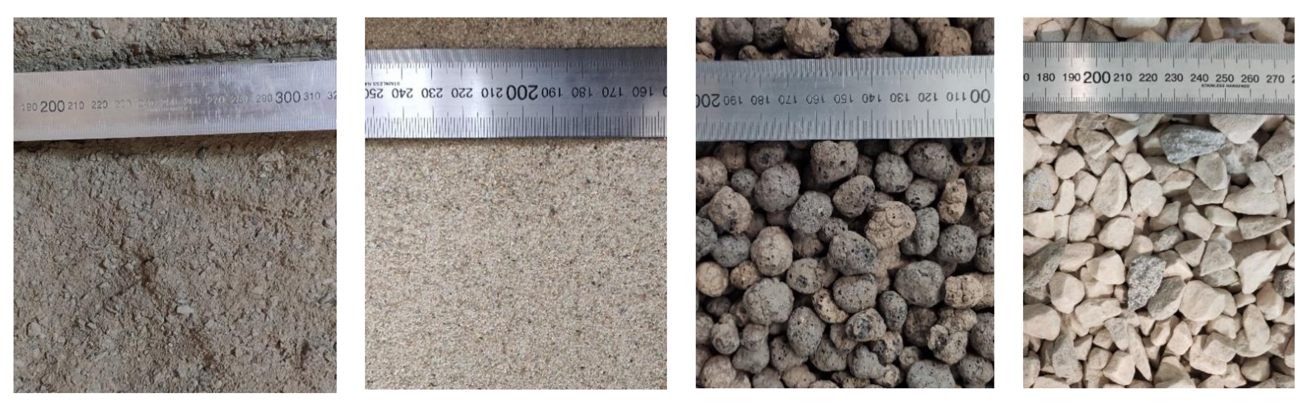
• Syar sand, a Martian regolith analog, was selected due to its high cohesion typical for surfaces of Mars, Moon, and smaller celestial bodies;
• Quartz sand, contrary to Syar, the quartz sand is incohesive; selected because it provides a good reference which can be easily reproduced;
• Expanded clay, selected due to its mimic of lightweight and sharp edges;
• Quartz aggregate, selected due to their higher density in contrary to expanded clay.

As mentioned previously, the primary concern of this research was the measurement of the energy dissipation coefficients when acting perpendicular to the surface. It constitutes a reference to other angles of approach that may be considered in the future. To indicate the possible change of energy dissipation in lateral hops, a set of three runs on quartz sand with a round foot (configuration #1) was also conducted at a 20° tilt angle. Both configurations, perpendicular and tilted, are shown in Figure 6. The tilt angle of 20° was purposely selected since this is the maximum operational angle at which we expect Hopter to operate, and therefore greater angles were of no interest.

3.5. Description of the MSC Adams Model for BB-0B

The test model was reproduced in MSC Adams software, a dedicated tool for numerical multibody analysis. The kinematics and dynamics matrices are produced within the software, and hence it is not mandatory to provide the analytical equations. Additionally, the model was validated through a simplified analytical model described in Section 3.2 and demonstrated in Figure 9. Details of the model are shown in Figure 15. The geometry and inertias were calculated as listed in

Table 3. Measured and calculated inertias of the BB-0B.

Component	Config. #0	Config. #1	Config. #2	Config. #3	Config. #4	Units
Foot	none	113.6	299.5	216.9	247.0	g
Actuating leg (without foot)	1060					g
Springs with guide sleeves	351.7					g
Stiffeners	1077.0					g
Actuator	989.38					g
Adapter	1283.5					g
Arm	1938.5					g
Rotational axis	888.7					g
Actuating leg’s moment of inertia w.r.t. rotational axis (Ileg)	3.912	4.271	4.860	4.599	4.694	kg m2
Full BB-0B’s moment of ineria w.r.t. rotational axis (Itotal)	14.679	15.039	15.628	15.366	15.462	kg m2
C1 coefficient (ratio of Ileg/Itotal)	26.6%	28.4%	31.1%	29.9%	30.4%	-

. The center of mass was located at a distance L_CoM equal to 1413 mm and measured with accuracy better than 10 mm, which in this scale of the model is less than 1% of potential error and therefore considered acceptable.

Analysis conditions and assumptions:

• The friction in the bearing of the main hinge (the rotational axis) was measured and is about 0.012 Nm. Therefore, energy losses are proven negligible at the angles measured during the test (less than 15° of the angular movement).
• The contact between the actuating leg and the surface and between the spring sleeves and the body part is defined with the following parameters: stiffness 10⁵ N/mm and force exponent 2.2. It is considered a relatively rigid contact. The minimal damping factors were introduced only to reduce the numerical uncertainties in the analysis.
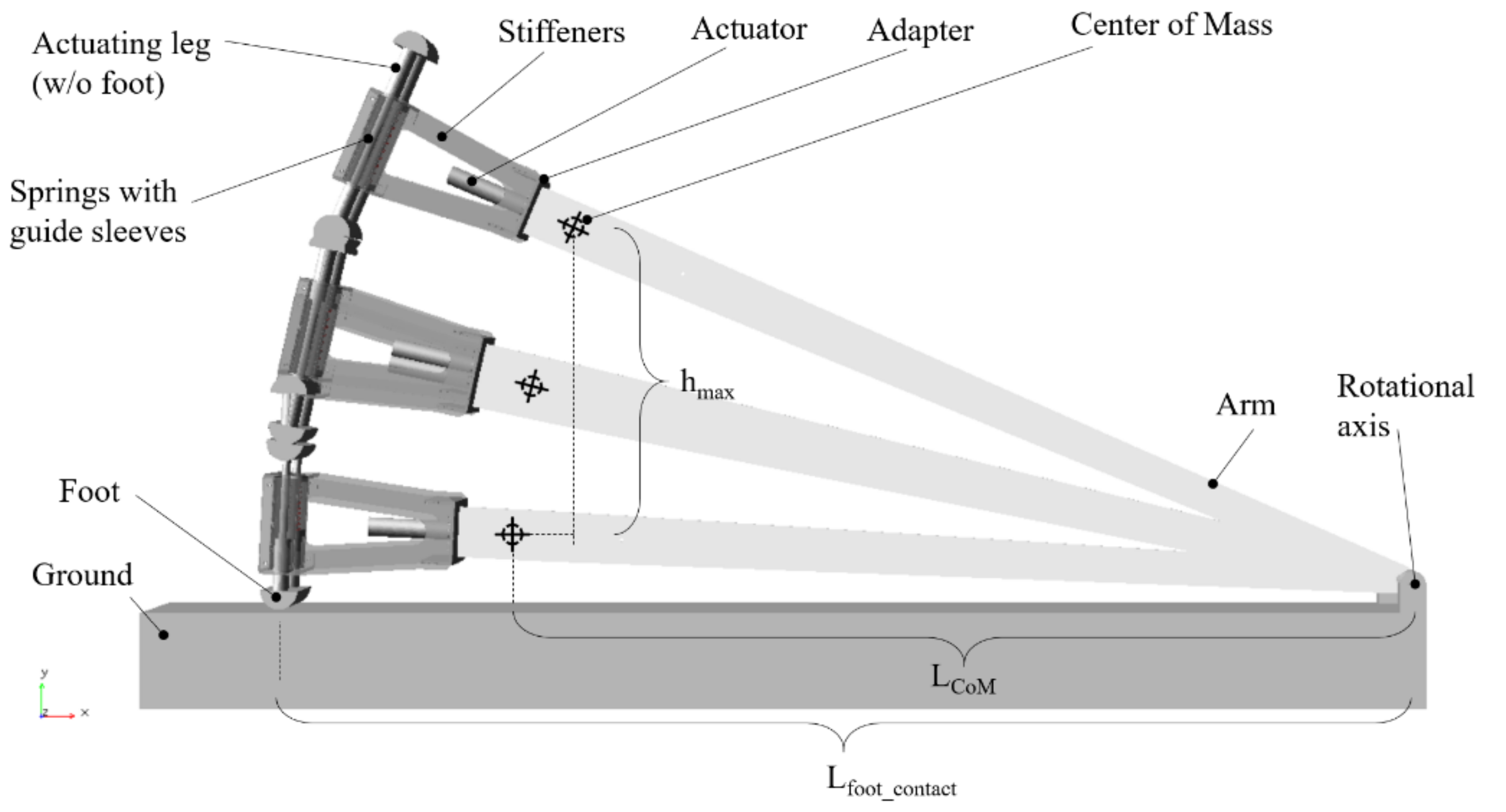
• The goal of the analysis is to determine the E_{jump_total} defined in Figure 7 to feed it in Equation (2), so we are looking for pure energy and assume the losses and dissipations are negligible as described previously in Section 3.3. The top position of the center of mass (h_max) was determined from the analysis and used to calculate the E_{jump_total} = E_{pot_analysis}.
• In the numerical model, the spring displacement was constant (contrary to the actual model). Therefore, the preload and stiffness coefficient had to be adjusted each time for each run of the analysis to provide the released energy of E_used as described in Section 3.2. A minimal damping factor was added in the spring to eliminate numerical errors and allow the system to settle with time.

4. Results

Eighty jumps were conducted in total, among which 54 were accepted for further analysis, while the remaining 26 had configuration or boundary conditions errors. The list of the test runs and related input data is available at the link provided in Supplementary Materials. The jumps were conducted with energies E_spr in the range of 15.3–24.0 J, with total reaction force F_spr on the springs ranging from 970 to 1210 N.

The results achieved can be displayed from the following perspectives:

• Validation of the coefficient C₁ (efficiency of the system determined by the mass distribution) and confirmation of the applicability of the analysis model as described in Section 3.2;
• Determination of coefficient C_{2_ref} (average losses of energies in the mechanism—e.g., friction—for reference jumps);
• Determination of coefficient C₃ (factor of energy dissipation with the surface);
• Results for a relation between foot-pad geometries and energy dissipation;
• Implications of other observations that may impact the robot’s displacement strategies, i.e., rapid compaction of cohesive material below the hopping robot or probing the surface before taking a large leap;
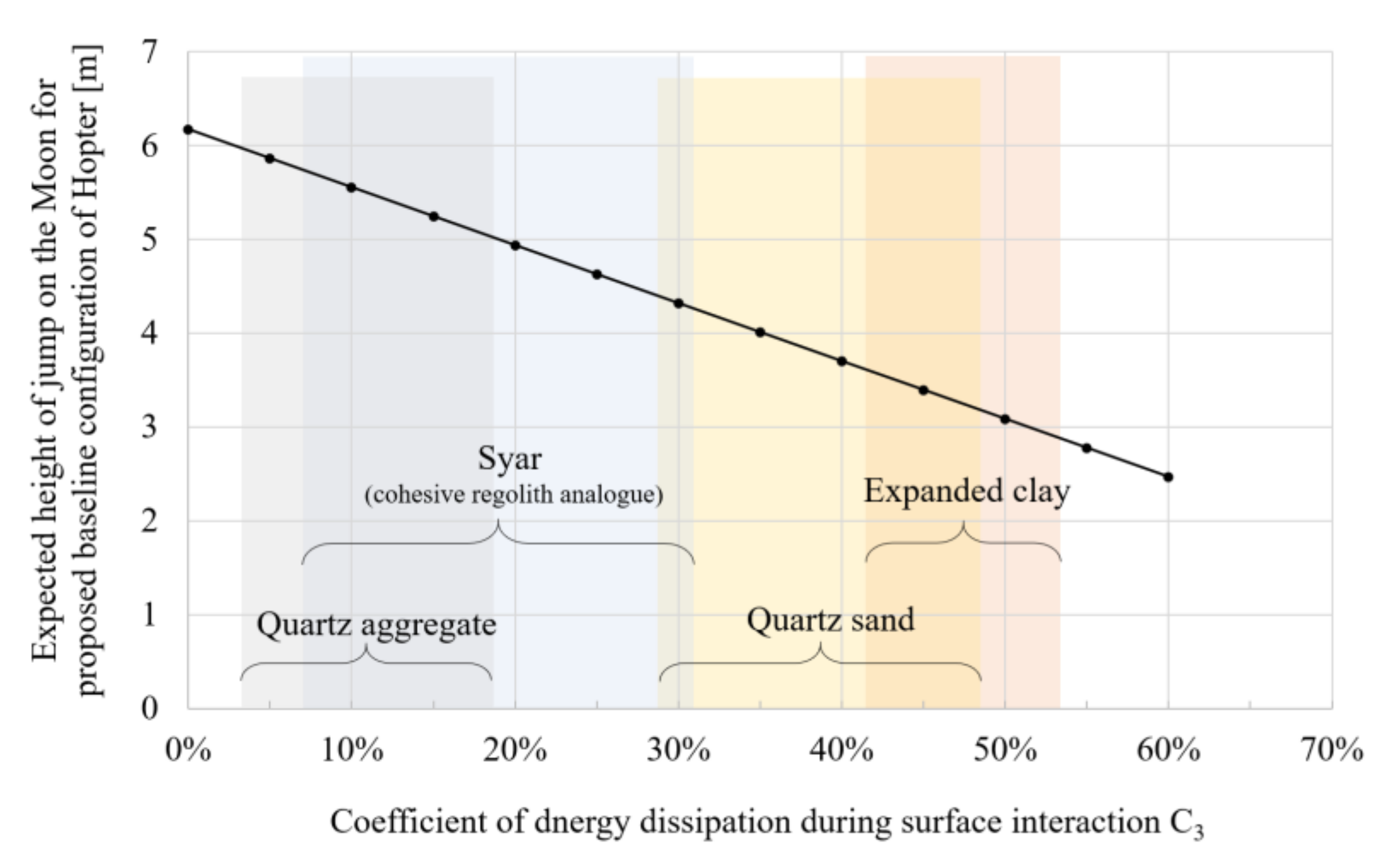
• Projections of maximum height of jump for Hopter case study;
• Results for reverse analysis and mean absolute error calculations as potential feedback for the robot’s trajectory planning.

4.1. Results of C₁ (Based on Analysis) and Defining C_{2_ref} for Reference Jumps

The achieved results of coefficients C₁ and C₂ are summarized for each test configuration in

Table 4. Results synthesis of the average coefficients C₁ and C₂.

Configuration	Average C1	Expected C1	Coefficient C2 (*)
#0	26.8% (25.6–30.2%) (based on 5 runs)	26.6%	2.6% (0.0–5.7%) (based on 5 ref runs)
#1	27.9 % (25.4–29.7%) (based on 35 runs)	28.4 %	5.9% (1.1–16.4%) (based on 11 ref runs)
#2	30.1% (30.07–30.13%) (based on 4 runs)	31.1%	7.2% (based on 1 ref run)
#3	29.0% (28.95–29.03%) (based on 6 runs)	29.9%	3.8% (based on 2 ref runs)
#4	29.6% (29.32–29.92%) (based on 4 runs)	30.4%	3.1% (based on 1 ref run)

(*) Average C₂ across all reference jumps is 4.8% (range: 0.0–16.4%) (based on 20 reference runs).

. The average C₁ results from the analysis run from Section 3.3, done for each actual jump of BB-0B and calculated with Equation (2). The expected C₁ is estimated as outlined in Section 3.2, Equation (1). The C₁ can be determined for each of the 54 test runs (regardless of the surface type). The results for C₁ show consistency with the simplified model with a mean absolute error of 3.4%, which is considered a satisfactory result.

The coefficient C₂ (interpreted as average internal energy losses in the mechanism) is averaged across each configuration of the BB-0B. It is calculated only for reference jumps on solid surfaces. Depending on the configuration used, they are in the range of 2.6–7.2% (average 4.8% for all runs). This value is considered moderate, and additional effort needs to be focused on developing the mechanism for the full-scale model to make sure this coefficient is lower than 5% in all cases. The components that contribute to that energy loss are listed previously in Table 1.

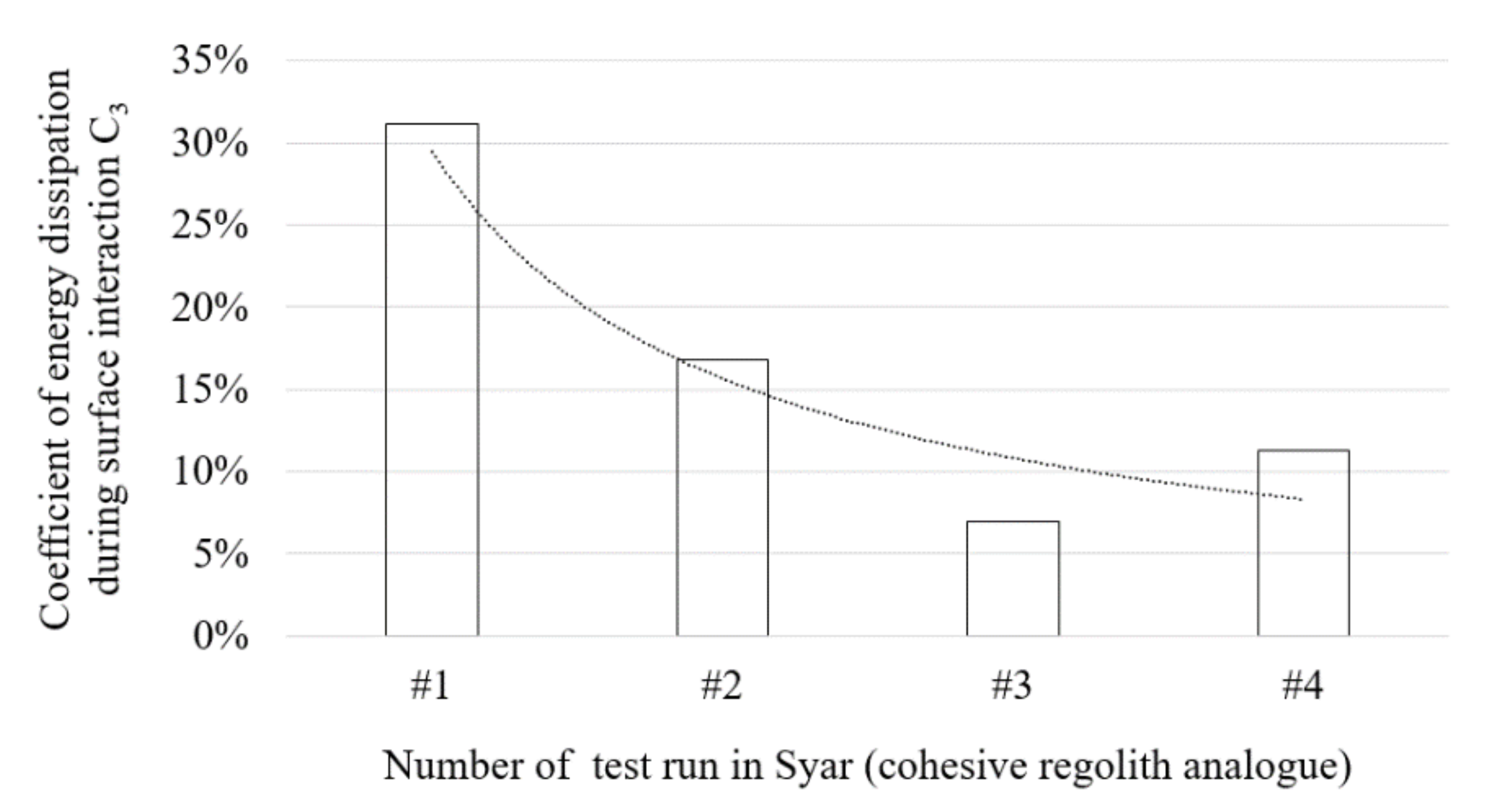
4.2. Results of C₃ for Jumps on the Non-Solid Surfaces

The aggregated data for the results of the coefficient C₃ are provided in

Table 5. Results synthesis for calculations of coefficient C₃.

Surface Type	Foot and Testbed Inclination	C3 Average (Range) for C2_ref_direct	C3 Average (Range) for C2_ref_average	No. of Runs	Density [kg/m3] (as in Table 2)
Syar	Foot: Config 1 (round) Angle: 0°	18.2% (7.2–31.3%)	18.1% (7.0–31.2%)	5	2010
Quartz sand	Foot: Config 1 (round) Angle: 0°	35.9% (29.3–47.2%)	38.8% (31.7–47.9%)	6	1840
Quartz sand	Foot: Config 1 (round) Angle: 20°	58.1% (51.0–68.9%)	57.9% (50.7–68.7%)	5	1840
Quartz sand	Foot: Config 2 (small flat) Angle: 0°	42.4% (34.7–47.9%)	43.9% (36.4–49.2%)	3	1840
Quartz sand	Foot: Config 3 (medium flat) Angle: 0°	26.3% (23.5–32.2%)	25.6% (22.8–31.5%)	4	1840
Quartz sand	Foot: Config 4 (large flat) Angle: 0°	15.1% (9.8–21.4%)	13.6% (8.2–20.0%)	3	1840
Expanded clay	Foot: Config 1 (round) Angle: 0°	46.0% (41.9–52.9%)	44.4% (40.2–51.6%)	4	270
Quartz aggregate	Foot: Config 1 (round) Angle: 0°	11.4% (6.4–19.1%)	8.8% (3.7–16.8%)	4	1700

. Where applicable, the average values were calculated and ranges were provided. The C₃ factor determines the amount of the effective jump energy E_{jump_effective} that was dissipated during the reaction with the surface. As derived in Appendix B, knowledge about C_{2_ref} is needed to calculate the C₃ correctly. There are two approaches, both presented in the table, where we use for either (1) the C₂ defined directly for the reference jump that was executed before the runs on a specific surface (C_{2_ref_direct}) or (2) for C₂ calculated against all reference run (C_{2_ref_average}). Remarkably, coefficient C₃ should be considered a property of a pair of objects (here, actuating leg and the surface) rather than just surface property. To demonstrate that, we obtained additional results for C₃ for jumps in quartz sand using three footpads with variable surface area. As seen in Table 5 and shown in Figure 16, the C₃ improves significantly with the surface area. It is reasonably justified that the dissipation needs tend towards 100% for surface area tending to zero. As expected, the round foot (config. #1) provides a dissipation coefficient smaller than the small flat foot (config. #2) yet larger than the medium flat foot (config. #3). Generally, those results may be considered for scaling laws in tailoring the surface area of the footpads for the best performance in the given geometrical constraints. Directional control in hopping robots requires changing the angle of approach of the actuating leg. Additional tests were conducted for a tilted configuration at a 20° angle in quartz sand. The angle corresponds to the maximum actuation angle in Hopter. The results suggest that the dissipation coefficient increases by a factor of 1.5 for a tilted actuation (from an average 39% to 58%). The change is greater than it would result from cosine function as would normally be expected on a rigid surface without slip.

4.3. Other Observations

Significant observations were made on jumping on Syar. Even though the jumps on Syar were limited only to 5 runs, a clear tendency was observed in which the coefficient C₃ decreased with each jump. This is important since Syar is an example of a cohesive regolith analog, and similar behavior may be expected on planetary surfaces. The C₃ factor for the sequence of the first four jumps is plotted in Figure 17 (for the fifth run the Syar was loosened again). The rapid change of dissipation coefficient may suggest that a cohesive material may get easily compacted, which may be used as a help in displacement strategies, e.g., conducting several minor jumps in place before taking a major jump forward. Apart from cohesiveness, particle size and shape distributions, which are much wider in Syar sand than in other investigated materials, should also play a major role in this effect. Such distributions allow porous space to be filled with the dry material instead of being displaced around the hopper’s foot.

The behavior of actuating leg and the surface were captured on recordings from a high-speed camera. For friable materials (e.g., quartz sand and expanded clay), the impulse force in jumps with configuration #1 was fluidizing the particles and generating a visible shock wave on the surface. The video showing the slow-motion movement on the surfaces is available at the link provided in Supplementary Materials. Video frames before and after the jump are shown in Figure 18, Figure 19, Figure 20 and Figure 21. Noticeably, configurations with flat footpads (i.e., configurations #3, #4 with the enlarged foot with the additional rim as shown in Figure 13) were encapsulating the movement of the quartz sand grains in the area directly below the foot, as seen partially in Figure 20 and Figure 21.

4.4. Results for Reverse Analysis and Projection of the Results to the Hopter Case Study

The principle of controlling any hopping robot over uncertain terrain would require a continuous update of the C₃ coefficient to adapt the trajectory planning to variable surface conditions. In this reverse analysis, we used the identified average C₃ coefficients to feed back the numerical model using Equation (7) to calculate expected performance and calculate mean absolute errors of the method. The analysis is inspired by [27]. The values are shown in Figure 22, and the MAE is summarized in

Table 6. Summary of average mean absolute errors.

Description	No. of Runs	MAE
Syar @ 0deg	5	8.6%
Quartz sand @ 0deg	16	7.1%
Quartz sand @ 20deg	5	11.7%
Expanded clay @ 0deg	4	7.1%
Quartz aggregate @ 0deg	4	3.7%
Total	34	7.6%

. The relative error is satisfactory (average 7.6%), given the small number of trials. It is anticipated that this method of surface energy dissipation identification may be a promising approach for reducing uncertainties in trajectory planning in planetary underactuated robots. Mainly, it would not be required to invest additional mass budget for additional force gauges sensors, but just interpret the adequate energy of the hop to identify the surface.

Having calculated energy coefficients C₁, C₂, C₃, we can eventually combine the model from Section 3.2 and Section 3.3 and the test results and represent them in terms of the expected maximum height of the vertical jump (h_max) of Hopter on the Moon (Figure 23). The hopper baseline is 10 kg, with 3 kg for legs and C₁ = 30% (the mass of the springs is distributed 50:50 between the legs and the platform). The coefficient of the mechanism losses during a jump is measured, and on average C_{2_ref_avarage} = 4.8%. The jump height decreases linearly with surface energy coefficient C₃, which is the horizontal axis of the plot.

5. Discussion

5.1. Lessons Learned

Several tests on various surfaces were conducted using a highly energetic actuator suitable for planetary underactuated hopping robots. In the proposed design, the floating spring principle was introduced (Figure 4), which is successfully tested on a prototype, demonstrating that we can achieve an acceptable efficiency level (average energy losses, C₂ factor, only about 4.8%). The use of volume and mass is optimal since only one set of springs is used in both directions (instead of two sets of springs, one for each actuation direction). The results are put in the context of the exemplary Hopter case study for lunar application to narrow down its estimated maximum height of jump to between 3–6 m high depending on the surface type. This is a promising result for a robot of which the objective is to hop over obstacles order of magnitude larger than itself.

The presented methodology allows for a combination of the numerical model with the actual system. It was successfully demonstrated on a unidirectional system that it could be utilized to predict its performance under limited runs on a given surface with an average mean absolute error of 7.6%. Furthermore, the energy approach is taken, which greatly simplifies the measurements; modeling is limited to a rigid surface (since the contact dynamics are indexed) and allows the use of the robot’s internal sensors that are already available on board a typical robot. The only parameters needed for the utilization of this method are:

• Actuators input energy, controlled by measurement of a deflection of the springs;
• The effective kinetic or potential energy of the hopping system, which can be determined by either measurement of the height of the jump (as done here but may be tricky for planetary application) or time of travel between actuators trigger and the first contact with the ground (i.e., by monitoring internal accelerometer). The latter is sufficient since the physics of projected vertical motion are well known.

The results provided in this article are essential since the available data addressing dissipation energy for space hopping platforms on various surfaces are limited and mostly related to recent hopping demonstrators in the Hayabusa2 mission [29,38]. In such investigations, Bekker or RFT modelings were used to simulate interaction with soils, and soil parameters were often simplified with a single empirical coefficient. Our research results provide valuable and specific information about energy dissipation (defined by coefficient C₃), which for vertical hops may vary in the range of 4% to 53% of the direct jump energy depending on the surface type. The highest dissipation was experienced on expanded clay (range: 40–53%), most probably attributed to its high porosity and brittleness. The lowest dissipation was measured on quartz aggregate (range: 4–19%), probably due to the hardness of the grains and their shape, which favors interlocking with each other. An interesting result was demonstrated for Syar, which increased its compaction very quickly and hence reduced the energy dissipation around 3 times in just four jumps performed in one place. This is a significant observation since a highly cohesive material like Syar may be expected on the lunar surface. This knowledge will help to improve the adaptive displacement strategies of hopping robots, which may use it to enhance trajectory planning and jump accuracy by compacting or probing the surface with a few preliminary jumps or hammerings before taking the large leap.

Scaling laws can be inferred from the energy dissipation coefficient determined against various surface areas (54–257 cm²) and shapes (flat and rounded) of the footpads on quartz sand. It was shown that an increase of the area by 4.8 times could reduce the dissipation factor ca. 3 times in the given condition. The measurement of dissipation energy coefficient for the tilted angle of approach was also demonstrated (increases ca. 1.5 times when changing from 0° to 20°).

In addition to the quantitative information, the direct methodology was validated on the 1-D system that may also be used in full-scale models of hopping robots. A proposal of such a recurrent algorithm is shown in Figure 24, where the calibration phase and in-field phase are distinguished. The calibration phase needs to take place before the actual field operation. The resulting coefficient of system efficiency (C₁) and coefficient of internal energy losses (C_{2_ref}) are identified in this phase. The control strategy applies for the infield phase in which surface dissipation coefficient (C₃) can be determined. [39] studied a similar 1-D system hopping on the granular media and suggests an implemented hopping control system extends to multipedal systems. In such a system, a simple open-loop control system is proposed. Essentially, during the flight phase, the jumping trajectory is not controlled. The data of the energy dissipation can be post-processed after the hop and used as an input for the trajectory planning of the next hop.

In comparison to [39], where a granular media model is considered to calculate the resistance of the soil, our approach takes into account indexing of the ground properties. The control strategy and hopping accuracy can be enhanced by the surface probing that can index the surface energy dissipation coefficients to minimize the hopping error. In the future, one can consider machine learning techniques to enhance the robot’s performance on the unknown surface, e.g., [40,41].

While the robot is operating, a catalog of expected jump performances may be used for regolith prospecting (helping determine, e.g., types of surfaces, density, cohesion, hardness, etc.) It is essential in the scope of in situ planetary exploration, where the scientific payload is limited and operations are done only in relatively unknown and extreme environments. There are several examples of how the regolith properties could be collected from dynamic interaction with the surface. Those are, for instance, Philae comet landing [42], MUPUS experiment [43], Hayabusa touch-and-go operation [44] and Deep Impact [45], or the one studied for Spacecraft/Rover Hybrids [46]. There are also numerous studies showing analysis of the interaction of the rover’s wheel with the surface to determine its properties, e.g., [47]. As in those examples, capturing the performance of the hopper is likely to help to identify surface types and properties by doing reverse analysis of its performance. However, this is open for future work.

Additionally, in this research, we could not demonstrate any strong correlation between the bulk density of a material and energy dissipation coefficient during surface interaction (C₃). Therefore, the number of test runs would need to be significantly increased with various other analogs. A dedicated (and different from presented here) methodology should also be implemented to conduct such research. However, it is visible in Figure 23 that the highest dissipation is experienced for the lightest material (i.e., expanded clay), which is in line with expectations.

It shall also be highlighted that the resulting factors for energy dissipation were measured in Earth’s gravity. At the same time, it is expected that the surface properties of granular materials may change with gravity. Still, the achieved results are essential and narrow down the uncertainties and risks to specific ranges of quantitative data that were not available at all previously. Furthermore, testing in simulated reduced gravity is not trivial and is considered an open matter for future work (as pointed in Section 5.2).

5.2. Open Matters and Future Work

The number of trials performed in this research was limited to validate the methodology of recurrent identification of energy dissipation at surface interaction. In the future, more statistical data should be characterized against various parameters and properties of such soils (e.g., cohesion, bearing capacity, grain size, relative density, shear strength). Such a database of information can be used to improve reverse analysis and interpretation of which kinds of soil the robot is traversing, knowing that energy dissipation is measured. Unfortunately, trials towards that statistical database are rarely done. Such operation with the soil, regolith and rocks requires additional efforts linked to sample preparation (usually large amounts of rocky and granular materials) and safety aspects (e.g., dust generation and heavy equipment).

From the perspective of the mechanical design, the presented test results indicate the need to improve the actuating mechanism in two aspects. Firstly, the energy loss in the mechanism is relatively low but not negligible, and the total energy accumulated in the springs needs to be higher to compensate for that loss. Secondly, the energies that need to be accumulated in the mechanism require significant amounts of force that elastically deflect the actuating mechanism itself (left side of Figure 7), which also reduces the effective jump energy; therefore, the actuating mechanism needs to be upgraded to improve the stiffness of the components.

Another aspect of the presented research is that the conducted tests were limited to normal conditions and only one component of the system, which is the actuating mechanism and actuating leg. As the technology readiness level (TRL) of this system increases (definitions of TRL can be found in [48]), it is typical for the next steps of developing space mechanisms and systems to include testing against relevant environmental conditions (i.e., extreme temperature, vacuum, reduced gravity). Naturally, such conditions are not trivial to replicate, and dedicated thermal vacuum chambers are needed. Testing for reduced gravity is even more challenging and rather unlikely to be tested on Earth unless advanced means are taken, e.g., 0 g flight campaigns [36] or 3-D off-loading systems [27].

References

1. Castillo-Rogez, J.C.; Pavone, M.; Nesnas, I.A.D.; Hoffman, J.A. Expected science return of spatially-extended in-situ exploration at small Solar system bodies. In Proceedings of the 2012 IEEE Aerospace Conference, Big Sky, MT, USA, 3–10 March 2012. [Google Scholar] [CrossRef]
2. Nesnas, I.A.; Matthews, J.B.; Abad-Manterola, P.; Burdick, J.W.; Edlund, J.A.; Morrison, J.C.; Peters, R.D.; Tanner, M.M.; Miyake, R.N.; Solish, B.S.; et al. Axel and DuAxel rovers for the sustainable exploration of extreme terrains. J. Field Robot. 2012, 29, 663–685. [Google Scholar] [CrossRef]
3. Nesnas, I.A.; Kerber, L.; Parness, A.; Kornfeld, R.; Sellar, G.; Mcgarey, P.; Brown, T.; Paton, M.; Smith, M.; Johnson, A.; et al. Moon Diver: A Discovery Mission Concept for Understanding the History of Secondary Crusts through the Exploration of a Lunar Mare Pit. In Proceedings of the 2019 IEEE Aerospace Conference, Big Sky, MT, USA, 2–9 March 2019. [Google Scholar] [CrossRef]
4. Yoshimitsu, T.; Kubota, T. Engineering challenges and results by MINEVRA-II asteroid surface rovers. J. Robot. Soc. Jpn. 2020, 38, 754–761. [Google Scholar] [CrossRef]
5. Kemurdzhian, A.; Bogomolov, A.; Brodskii, P.; Gromov, V.; Dolginov, S.; Kirnozov, F.F.; Kozlov, G.V.; Komissarov, V.I.; Ksanfomality, L.V.; Kucherenko, V.I.; et al. Study of Phobos’ Surface with a Movable Robot. In Scientific and Methodological Aspects of the Phobos Study; Space Research Institute: Moscow, Russia, 1986; pp. 357–367. [Google Scholar]
6. Reid, R.G.; Roveda, L.; Nesnas, I.A.D.; Pavone, M. Contact Dynamics of Internally-Actuated Platforms for the Exploration of Small Solar System Bodies. In Proceedings of the i-SAIRAS, Montreal, QC, Canada, 17–19 June 2014. [Google Scholar]
7. Clark, B.C.; Sunshine, J.M.; A’Hearn, M.F.; Cochran, A.L.; Farnham, T.L.; Harris, W.M.; McCoy, T.J.; Veverka, J. Comet Hopper: A Mission Concept for Exploring the Heterogeneity of Comets. Proceedings of LPI Asteroids, Comets, Meteors, Baltimore, MD, USA, 14–18 July 2008. [Google Scholar]
8. Fiorini, P.; Bovo, F.; Bertelli, L.; Munteanu, M.G. Solving the landing problem of hopping robots: The elastic cage design. In Proceedings of the ESA Workshop on Advanced Space Technologies for Robotics and Automation (ASTRA), Noordwijk, The Netherlands, 11–14 November 2008. [Google Scholar]
9. Lee, P.; Riedel, J.E.; Jones-Wilson, L.L.; Brandeau, E.J.; O’Farrel, C.; Gallon, J.C.P.R.S. Globetrotter: An airbag hopper for Mars surface and pit/cave exploration. In Proceedings of the LPI Ninth International Conference on Mars, Pasadena, CA, USA, 22–25 July 2019. [Google Scholar]
10. Landis, G.A.; Oleson, S.R.; Abel, P.; Bur, M.; Colozza, A.; Faller, B.; Fittje, J.; Gyekenyesi, J.; Hartwig, J.; Jones, R.; et al. Missions to Triton and Pluto using a Hopper Vehicle with In-Situ Refueling. In Proceedings of the 70th International Astronautical Congress (IAC), Washington, DC, USA, 21–25 October 2019. [Google Scholar]
11. Kalita, H.; Thangavelautham, J. Exploration of extreme environments with current and emerging robot systems. Curr. Robot. Rep. 2020, 1, 94–104. [Google Scholar] [CrossRef]
12. Mège, D.; Gurgurewicz, J.; Grygorczuk, J.; Wiśniewski, Ł.; Thornell, G. The Highland Terrain Hopper (HOPTER): Concept and use cases of a new locomotion system for the exploration of low gravity Solar System bodies. Acta Astronaut. 2016, 121, 200–220. [Google Scholar] [CrossRef]
13. Byl, K.; Byl, M.; Rutschmann, M.; Satzinger, B.; van Blarigan, L.; Piovan, G.; Cortell, J. Series-elastic actuation prototype for rought terrain hopping. In Proceedings of the IEEE International Conference on Technologies for Practical Robot Applications, Woburn, MA, USA, 23–24 April 2012. [Google Scholar] [CrossRef]
14. Batts, Z.; Kim, J.; Yamane, K. Design of a hopping mechanism using a voice coil actuator: Linear elastic actuator in parallel (LEAP). In Proceedings of the 2016 IEEE International Conference on Robotics and Automation (ICRA), Stockholm, Sweden, 16–21 May 2016. [Google Scholar] [CrossRef]
15. Bai, L.; Zheng, F.; Chen, X.; Sun, Y.; Hou, J. Design and Experimental Evaluation of a Single-Actuator Continuous Hopping Robot Using the Geared Symmetric Multi-Bar Mechanism. Appl. Sci. 2019, 9, 13. [Google Scholar] [CrossRef] [Green Version]
16. Ambrose, E.; Csomay-Shanklin, N.; Or, Y.; Ames, A. Design and Comparative Analysis of 1D Hopping Robots. In Proceedings of the 2019 IEEE/RSJ International Conference on Intelligent Robots and Systems (IROS), Macau, China, 4–8 November 2019. [Google Scholar]
17. Wilburn, G.; Kalita, H.; Thangavelautham, J. Development and testing of an engineering model of an asteroid hopping robot. In Proceedings of the International Astronautical Congress, Washington, DC, USA, 21–25 October 2019. [Google Scholar]
18. Kalita, H.; Schwartz, S.; Asphaug, E.; Thangavelautham, J. Mobility and Science Operations on an Asteroid Using a Hopping Small Spacecraft on Stilts. 2018. Available online: https://arxiv.org/abs/1801.09482 (accessed on 1 March 2021).
19. Oshashi, E.; Ohnishi, K. Hopping height control for hopping robots. Electr. Eng. Jpn. 2006, 155, 650–665. [Google Scholar]
20. Kobashi, K.; Bando, A.; Nagaoka, K.; Yoshida, K. Tumbling and Hopping Locomotion Control for a Minor Body Exploration Robot. In Proceedings of the 2020 IEEE/RSJ International Conference on Intelligent Robots and Systems (IROS), Las Vegas, NV, USA, 25–29 October 2020. [Google Scholar] [CrossRef]
21. Cherouvim, N.; Papadopoulos, P. Control of hopping speed and height over unknown rough terrain using a single actuator. In Proceedings of the IEEE International Conference on Robotics and Automation, Kobe, Japan, 12–17 May 2009. [Google Scholar] [CrossRef]
22. Hyon, S.H.; Emura, T.; Mita, T. Dynamics-based control of a one-legged hopping robot. Inst. Mech. Eng. Part I J. Syst. Control Eng. 2003, 217, 83–98. [Google Scholar] [CrossRef]
23. Zabihi, M.; Alasty, A. Dynamic stability and control of a novel handspringing robot. Mech. Mach. Theory 2019, 137, 154–171. [Google Scholar] [CrossRef]
24. Yesilevskiy, Y.; Gan, Z.; Remy, C.D. Energy-optimal hopping in parallel and series elastic 1D monopods. J. Mech. Robot. 2018, 10. [Google Scholar] [CrossRef] [Green Version]
25. Kalveram, K.T.; Häufle, D.; Grimmer, S.; Seyfarth, A. Energy management that generates hopping: Comparison of virtual, robotic and human bouncing. In Proceedings of the International Conference on Simulation, Modelling and Programming for Autonomous Robots, Darmstadt, Germany, 15–16 November 2010. [Google Scholar]
26. Chen, G.; Tu, J.; Ti, X.; Hu, H. A Single-legged Robot Inspired by the Jumping Mechanism of Click Beetles and Its Hopping Dynamics Analysis. J. Bionic Eng. 2020, 17, 1109–1125. [Google Scholar] [CrossRef]
27. Hockman, B.; Reid, R.G.; Nesnas, I.A.D.; Pavone, M. Experimental Methods for Mobility and Surface Operations of Microgravity Robots. In 2016 International Symposium on Experimental Robotics; Springer Proceedings in Advanced, Robotics; Kulić, D., Nakamura, Y., Khatib, O., Venture, G., Eds.; Springer: Cham, Switzerland, 2017; Volume 1. [Google Scholar] [CrossRef]
28. Moritz, C.T.; Farley, C.T. Human hoppers compensate for simultaneous changes in surface compression and damping. J. Biomech. 2004, 39, 1030–1038. [Google Scholar] [CrossRef] [PubMed]
29. Sakamoto, K.; Otsuki, M.; Kubota, T.; Morino, Y. RFT-Based Analysis of Mobility Performance of Hopping Rover on Soft Soil for Planetary Exploration. In Proceedings of the 13th International Symposium on Artificial Intelligence, Robotics and Automation in Space (i-SAIRAS 2016), Beijing, China, 20–22 June 2016. [Google Scholar]
30. Sakamoto, K.; Otsuki, M.; Kubota, T.; Morino, Y. Hopping Motion Estimation on Soft Soil by Resistive Force Theory. J. Robot. Mechatron. 2017, 29, 895–901. [Google Scholar] [CrossRef]
31. Vasilopoulos, V.; Paraskevas, I.S.; Papadopoulos, E.G. Monopod hopping on compliant terrains. Robot. Auton. Syst. 2018, 102, 13–26. [Google Scholar] [CrossRef]
32. Maeda, T.; Kunii, Y.; Yoshikawa, K.; Otsuki, M.; Yoshimitsu, T.; Kubota, T. Design of shoe plate for small hopping rover on loose soil. In Proceedings of the 2018 IEEE Aerospace Conference, Big Sky, MT, USA, 3–10 March 2018. [Google Scholar] [CrossRef]
33. Roberts, S.; Koditschek, D.E. Mitigating energy loss in a robot hopping on a physically emulated dissipative surface. In Proceedings of the International Conference on Robotics and Automation (ICRA), Montreal, QC, Canada, 20–24 May 2019. [Google Scholar]
34. Wiśniewski, Ł.; Grygorczuk, J.; Węclewski, P.; Mege, D.; Gurgurewicz, J.; Zielińska, T.; Gritsevich, M.; Peltoniemi, J. Mobility and terrain accessibility analysis for Hopter—An underactuated mobile robot for planetary exploration. In Proceedings of the ESA Workshop on Advanced Space Technologies for Robotics and Automation (ASTRA), Leiden, The Netherlands, 20–22 June 2017. [Google Scholar]
35. Wiśniewski, Ł.; Grygorczuk, J.; Mege, D.; Gurgurewicz, J. Design Features of Novel High Energy Impulsive Drive of Underactuated Mobile Robot for Planetary Exploration. In Proceedings of the 17th European Space Mechanisms and Tribology Symposium, Hatfield, UK, 20–22 September 2017. [Google Scholar]
36. Marshall, J.P.; Hurley, R.C.; Arthur, D.; Vlahinic, I.; Senatore, C.; Iagnemma, K.; Trease, B.; Andrade, J.E. Failures in sand in reduced gravity environments. J. Mech. Phys. Solids 2018. [Google Scholar] [CrossRef] [Green Version]
37. Karapiperis, K.; Marshall, J.P.; Andrade, J.E. Reduced Gravity Effects on the Strength of Granular Matter: DEM Simulations versus Experiments. J. Geotech. Geoenviron. Eng. 2020, 146. [Google Scholar] [CrossRef]
38. Maeda, T.; Kunii, Y.; Yoshikawa, K.; Otsuki, M.; Yoshimitsu, T.; Kubota, T. Hopping simulation for small rover using regolith model considering the result of vacuum and small gravity flight experiment. In Proceedings of the i-SAIRAS 2018, Madrid, Spain, 4–6 June 2018. [Google Scholar]
39. Hubicki, C.M.; Aguilar, J.J.; Goldman, D.I.; Ames, A. Tractable terrain-aware motion planning on granular media: An impulsive jumping study. In Proceedings of the 2016 IEEE/RSJ International Conference on Intelligent Robots and Systems (IROS), Daejeon, Korea, 9–14 October 2016. [Google Scholar] [CrossRef]
40. Dong, Y.; Tang, X.; Yuan, Y. Principled reward shaping for reinforcement learning via lyapunov stability theory. Neurocomputing 2020, 393, 83–90. [Google Scholar] [CrossRef]
41. Kusano, Y.; Tsutsumi, K. Hopping height control of an active suspension type leg module based on reinforcement learning and a neural network. In Proceedings of the IEEE/RSJ International Conference on Intelligent Robots and System, Lausanne, Switzerland, 30 September–4 October 2002. [Google Scholar] [CrossRef]
42. Biele, J.; Ulamec, S.; Maibaum, M.; Roll, R.; Witte, L.; Jurado, E.; Muñoz, P.; Arnold, W.; Auster, H.-U.; Casas, C.M.; et al. The landing(s) of Philae and inferences about comet surface mechanical properties. Science 2015, 349, 6247. [Google Scholar] [CrossRef] [PubMed]
43. Spohn, T.; Knollenberg, J.; Ball, A.J.; Banaszkiewicz, M.; Benkhoff, J.; Grott, M.; Kührt, E.; Kossacki, K.J.; Marczewski, W.; Pelivan, I.; et al. Thermal and mechanical properties of the near-surface layers of comet 67P/Churyumov-Gerasimenko. Science 2015, 349, 6247. [Google Scholar] [CrossRef] [PubMed] [Green Version]
44. Yano, H.; Kubota, T.; Miyamoto, H.; Okada, T.; Scheeres, D.; Takagi, Y.; Yoshida, K.; Abe, M.; Abe, S.; Barnouin, O.; et al. Touchdown of the Hayabusa Spacecraft at the Muses Sea on Itokawa. Science 2006, 312, 1350–1353. [Google Scholar] [CrossRef]
45. A’Hearn, M.F.; Belton, M.J.S.; Delamere, W.A.; Kissel, J.; Klaasen, K.P.; McFadden, L.A.; Meech, K.J.; Melosh, H.J.; Schultz, P.H.; Sunshine, J.M.; et al. Deep Impact: Excavating Comet Tempel 1. Science 2005, 310, 5746. [Google Scholar] [CrossRef] [Green Version]
46. Wisniewski, L.; Reid, R.G.; Nesnas, I.A.; Chmielewski, A.; Grygorczuk, J. In Situ Measurements of Regolith Properties on Small Solar System Bodies using Spacecraft/Rover Hybrids. In Proceedings of the 69th International Astronautical Congress (IAC), Bremen, Germany, 1–5 October 2018. [Google Scholar]
47. Sullivan, R.; Anderson, R.; Biesiadecki, J.; Bond, T.; Stewart, H. Martian Regolith Cohesions and Angles of Internal Friction from Analysis of Mer Wheel Trenches. Proceedings of 38th Lunar and Planetary Science Conference, League City, TX, USA, 12–16 March 2007. [Google Scholar]
48. European Cooperation for Space Standarization. ECSS, ECSS-E-HB-11A Technology Readiness Level (TRL) Guidelines; ESA-ESTEC, Requirements & Standards Division: Noordwijk, The Netherlands, 2017. [Google Scholar]
Figure 1. Design visualization of Hopter, top of the cover, and one of the front legs are semi-transparent to show the interior arrangement.
Energies 14 04282 g001
Figure 2. Visualization of the actuator in a neutral position (left) and tensioned (right).
Energies 14 04282 g002
Figure 3. The actual implementation of the actuator in the prototype model (also called BB-0B).
Energies 14 04282 g003
Figure 4. Principle of compression of the drive springs suspension in BB-0B (floating spring).
Energies 14 04282 g004
Figure 5. (Left) representation of the BB-0B. (Right) cross-section through guides to show the realization of the concept in BB-0B.
Energies 14 04282 g005
Figure 6. (Left) The actual implementation of the compression springs suspension in the BB-0B testbed. (Right) Horizontal (0°) and inclined (20°) configurations of the testbed.
Energies 14 04282 g006
Figure 7. Energy contributions in the actuating mechanism and drive springs. The horizontal axis is mechanism (fmech) and drive springs deflection (fgrav + fused), the vertical axis is the drive spring reaction forces.
Energies 14 04282 g007
Figure 8. Schematics of the masses for the simplified analytical model. See Appendix A for more details.
Energies 14 04282 g008
Figure 9. Jumping efficiency factor ( C 1 * ) against mass ratio of the mass of legs (mlegs) to total mass of Hopter (Mtotal).
Energies 14 04282 g009
Figure 10. View over typical test scene of the BB-0B.
Energies 14 04282 g010
Figure 11. Two overlayed video frames showing actuating leg just before the jump and in the utmost height position (hmax).
Energies 14 04282 g011
Figure 12. From left: configuration #1 with a cylindrical 3D-printed foot in contact with quartz sand; configuration #2 actuating leg with a flat surface contact area same as config #1; configuration #3 with a flat surface contact area based on a width equivalent to the diameter of the round foot; configuration #4 with a flat foot with a contact area 4.8 times greater than contact area from the configuration #1 and #2.
Energies 14 04282 g012
Figure 13. Dimensions and details of the configurations #1, #2, #3 and #4. The extrusion of the shapes is 134 mm.
Energies 14 04282 g013
Figure 14. The type of surface materials used in the tests. From left: Syar, quartz sand, expanded clay, quartz aggregate.
Energies 14 04282 g014
Figure 15. The overlayed sequence of BB-0B jump in MSC Adams with indicated major components and geometry.
Energies 14 04282 g015
Figure 16. Dependence of the coefficient of surface energy dissipation against footpad surface area. The blue dots are results for configurations #2, #3 and #4. The orange triangle is a result for the rounded footpad (config. #1).
Energies 14 04282 g016
Figure 17. Results of the measurement of coefficient C3 for subsequent jumps on Syar surface.
Energies 14 04282 g017
Figure 18. Jump in Syar with the foot in configuration #1.
Energies 14 04282 g018
Figure 19. Jump in quartz sand with the foot in configuration #2.
Energies 14 04282 g019
Figure 20. Jump in quartz sand with the foot in configuration #3.
Energies 14 04282 g020
Figure 21. Jump in quartz sand with the foot in configuration #4.
Energies 14 04282 g021
Figure 22. Test measurements (htest) compared to predicted height of jump from analysis (hanalysis).
Energies 14 04282 g022
Figure 23. Exemplary maximum height of jump (hmax) for the 10 kg Hopter in lunar gravity against the measured energy dissipation coefficients (here, for the purpose of the exercise, assuming the coefficient does not change with gravity). The semi-transparent areas are the ones calculated based on the test data.
Energies 14 04282 g023
Figure 24. Structured control algorithm for trajectory planning, including energy dissipation coefficients.
Energies 14 04282 g024