Assessing Economic Impacts of Thailand’s Fiscal Reallocation between Biofuel Subsidy and Transportation Investment: Application of Recursive Dynamic General Equilibrium Model

Phomsoda, Korrakot; Puttanapong, Nattapong; Piantanakulchai, Mongkut

doi:10.3390/en14144248

Open AccessArticle

Assessing Economic Impacts of Thailand’s Fiscal Reallocation between Biofuel Subsidy and Transportation Investment: Application of Recursive Dynamic General Equilibrium Model

by

Korrakot Phomsoda

¹

,

Nattapong Puttanapong

²

and

Mongkut Piantanakulchai

^1,*

¹

Sirindhorn International Institute of Technology, School of Civil Engineering and Technology, Thammasat University, Pathum Thani 12120, Thailand

²

Faculty of Economics, Thammasat University, Bangkok 10200, Thailand

^*

Author to whom correspondence should be addressed.

Energies 2021, 14(14), 4248; https://doi.org/10.3390/en14144248

Submission received: 31 May 2021 / Revised: 28 June 2021 / Accepted: 9 July 2021 / Published: 14 July 2021

(This article belongs to the Section C: Energy Economics and Policy)

Download

Browse Figures

Versions Notes

Abstract

:

This study examined the economy-wide effects of reallocating the biofuel subsidy to invest in transportation using a recursive dynamics computable general equilibrium model. The constructed model consists of 35 sectors, 42 commodities, and 3 institutions (household, government, and the rest of the world). Three scenarios were simulated. In the first scenario, the subsidy of gasohol and biodiesel is completely removed, whereas, in the second and third scenarios, half of the removed subsidy is reallocated to finance investment in road freight transportation and road public transportation. The simulation results show that reallocating the biofuel subsidy to invest in road public transportation can lead to the highest long-term economic growth and has the lowest impact on the consumer price index (CPI). All findings suggest that policymakers should maintain continuous investment in transportation and prioritize this investment policy over the fuel price distortion scheme.

Keywords:

computable general equilibrium; investment; transportation; logistics; subsidy

1. Introduction

Since the implementation of the first Social and Economic Development Plan in 1961, transportation investment has continuously been one of the main targeted activities. Although road transportation is the main mode of domestic transportation and shipment, the coverage of the road network still lags behind the growing economic activities that influence vehicle ownership and transportation volume [1]. A comparison between the coverage of telecommunications and transportation facilities also indicated that the penetration of mobile phones per capita in Thailand is close to that in Japan, but transportation accessibility is roughly 10 times lower [2].

In addition to measurements of the road network (i.e., the total road length and its density), the efficiency and economic contribution of transportation have been regularly studied by the Office of the National Economic and Social Development Council (NESDC) and published in the Thailand Logistics Report [3]. The latest report indicated that between 2015 and 2019, the logistics costs per GDP of Thailand slightly declined from 13.9% to 13.4%. This ratio was still higher than the global average (10.7%) and the value for the Asia-Pacific region (12.7%). Similarly, the most recent Logistics Performance Index (LPI) of Thailand is 3.41, which ranks 32nd of 167 countries [4] and is still far from the values of OECD countries [5]. To resolve this shortcoming, the national strategic plan for logistics development was formulated, aiming to enhance Thailand’s logistics performance and expand facilities to enable multimodal transportation [6,7]. Specifically, this national policy concentrates on financing infrastructure investment [1,7] because transportation development can raise manufacturing productivity in the long run [2]. Moreover, the construction of roads and transportation facilities directly increases employment, demand for construction materials, and real estate investment [8,9].

From an alternative perspective, economic expansion has been concurrently increasing the volumes of domestic road transportation for many decades, which has subsequently induced the continuous growth in demand for fuels. To stabilize the domestic prices of fossil-based fuels amid the fluctuation of the global crude oil price, the oil fund was established in 2003 to function as a cross-fuel price subsidizer. However, in response to the rising concern regarding the economic efficiency and the sustainability of the fund, the government recently revised the oil fund legislation. The goal of the new act is to terminate the biofuel subsidy by the end of 2022.

By integrating the goals and the constraints of both the transportation investment policy and the fuel price scheme, this study aimed to examine the impacts of removing the biofuel subsidy and reallocating it to finance the investment in road transportation. A recursive dynamics computable general equilibrium model was the main research method, which enables the quantitative investigation of intertemporal economy-wide adjustments. Furthermore, a sensitivity analysis was conducted by varying the substitution coefficients to validate the stability of the main findings. Hence, these quantitative approaches enable the thorough hypothesis testing of formulating the feasible policy for offsetting the negative impacts of the fuel subsidy removal.

The paper is structured as follows: Section 1 introduces the background of this study, and Section 2 discusses previous literature related to Computable General Equilibrium (CGE) model and transportation investment simulations. Section 3 outlines the model’s main structure. Section 4 presents the results and discussion. Section 5 reports the key findings and suggests policy recommendations.

2. Materials and Methods

In Thailand, CGE studies have confirmed that the removal of biofuel subsidies will lead to an increase in economic growth in the long term [10,11,12]. These results are in line with previous studies in other countries [13,14]. In particular, the reallocation of the biofuel subsidy will be more beneficial than removing it without re-investment [12]. In the aspect of transportation, previous CGE studies have mainly emphasized the effects of investments in transportation infrastructure.

Korea developed a framework to estimate economic growth resulting from highway projects, and it was found that all projects were beneficial to GDP and export growth [15]. Furthermore, this model was extended to analyze the effect of the network of highway projects on the regional economy of Korea. The simulation found that highway development could reduce regional disparities [16]. In addition, the model was also applied to study different financial strategies. The results indicated that earmarked tax positively affected income growth and diminished regional income inequality more than the current tax system [17]. The finding related to inequality is similar to the result of a study in Poland that applied the regional dynamics CGE model to measure the impacts of transportation investments. It highlighted a disparity in road investment between regions, resulting in a decrease in real GDP and employment [18].

A study in the USA applied the CGE model to evaluate the public transportation stock. It revealed that road stock had the highest impact on GDP growth and social welfare. On the contrary, public transit and other ground passenger transportation had relatively negligible impacts on the economy [19]. The results of this study differ from those reported in an Iranian study, which used the CGE model to assess investment in transport infrastructure. The authors found that investment in the railway had the greatest impact on economic growth, while investment in roads could affect household welfare [20]. However, road infrastructure investment was still confirmed to affect economic growth [8,9,21,22,23].

In addition, a CGE model was developed by combining it with an engineering model called USAGE-Hwy to examine the economic impacts of highway investments. Simulations showed that with an increase in petroleum tax to finance highway and bridge expenditures, employment grew slightly in the short term, considerably increased in the middle term, and decreased in the long term [24].

Because our study is related to the transportation issue, several CGE studies are reviewed as follows. In Malaysia, a study demonstrated the effects of energy subsidy reform on the economy and the transportation sector. The results showed that real GDP and real investment would increase, while exports and imports would decrease. Moreover, the transportation sector was affected due to an increase in production costs, which affected total output and exports [13].

In Indonesia, a study on transportation investment using path analysis found that shifting the fuel subsidy led to GDP growth but decreased the transport multiplier, leading to inequality. The authors recommended two options for subsidy policy management, i.e., (1) cutting the fuel subsidy if the goal is income distribution or (2) cutting the fuel subsidy to invest in transport infrastructure if the goal is economic growth [25]. The financial CGE model was developed to analyze the effect of infrastructure investment projects on the economic system of Indonesia, and its results showed that government financing of transportation projects with tax revenue could have a greater impact on GDP than other financing methods [26]. A further study used the CGE model to examine the effect of reallocating the fuel subsidy to infrastructure investment. Its simulation outcomes indicated that the reallocation had positive impacts on economic growth but adversely affected income equality [27].

In our study, the main research question and method are similar to those of a South African study, which constructed a CGE model to simulate the reallocation of the fuel subsidy to support public transport services. The results indicated that unemployment was reduced, and the household income and economy increased [28]. This benefit of reallocation corresponds to the redistribution of a tax levy, proving that the government can decrease personal income tax and increase other taxes to balance its revenue [29]. Therefore, the additional government revenue resulting from the termination of biofuel subsidies should be distributed to invest in significant sectors to drive economic growth, especially transportation sectors with construction activity and other management projects that need capital to drive their productivities [19].

3. Methodologies

The standard CGE model used in this study was adopted from the Partnership for Economic Policy (PEP) [30]. The features of the model consist of four parts, which are described below. (The full details of equations, variables and coefficients of this model are shown in Appendix B).

3.1. Production Structure

Figure 1 presents the structure of production sectors that consist of three levels. The aggregate output combines a primary factor and intermediate commodity demand at the top level with a fixed proportion, called the Leontief (LEO) function. At the second level, the primary factor is the combination of labor and capital with the function of constant elasticity of substitution (CES). At the same level, the non-transport-energy and transport-energy commodities are integrated with LEO. Finally, there are four combinations mixed with CES at the lowest level. Because this study focused on the removal of the biofuel subsidy, we focused on two types of biofuel that can substitute each other, i.e., mixed biodiesel, which comprises mandatory biodiesel and optional biodiesel, and mixed gasohol, which is the combination of gasohol–gasoline (91/95/E10) and gasohol (E20/E85). Similarly, this study concentrated on reallocating the subsidy to invest in transportation sectors. Hence, we distinguished two types of transportation, i.e., freight transportation, which consists of railway and road freight transportation, and mass transportation, which includes railway passenger transportation and road public transportation.

Besides production sectors, household consumption plays a crucial role in driving the economy. The household consumption of goods and services follows the Stone–Geary utility function to maximize utility subject to budget constraints. The commodity price determines the investment demand. The commodity produced domestically has two selling options, i.e., supplying the domestic consumption or exporting in the form of international trade with constant elasticity of transformation (CET) (the values of elasticity of transformation parameters are shown in Appendix A). Finally, the commodity sold domestically is a combination between an import and the domestic commodity determined by CES’s function.

3.2. Database

The CGE model replicates the economy-wide market-based relationship among economic agents. The model is conventionally constructed based on the nationwide transaction data shown in the Social Accounting Matrix (SAM). In this study, the SAM comprises 35 sectors and 42 commodities, as exhibited in Table A1 (see Appendix A).

3.3. Dynamics Assumption

This study applied the recursive dynamic modeling technique to examine impacts over a 10-year period (2022–2031). Following the main structure suggested by the Partnership for Economic Policy (PEP) [30], the discrete intertemporal mechanism of capital accumulation is embedded in the CGE model, enabling medium-term and long-term simulations. (There is an alternative specification of dynamic simulation that allows for intertemporally optimizing behaviors of the economic agent [12,31]. However, several parameters for such specifications were unavailable for Thailand. Therefore, the recursive dynamic technique was selected.)

In addition to the endogenous dynamic process of capital accumulation, the growth rates of some dynamic variables were exogenously assigned, i.e., the depreciation rate, the elasticity of investment demand, population, exports, total investment, public investment, government expenditures, and productivity. The depreciation rate and the elasticity of investment demand were based on the conventional values suggested by previous studies [12,32]. The growth rates of the population, exports, total investment, public investment, and government expenditures were averaged from the official report published by the Office of the National Economic and Social Development Council [33]. The productivity was based on the historical trend estimated by the Office of Industrial Economics (OIE) [34,35] (the numerical details of these growth rates are shown in Appendix A).

3.4. Closure and Solution

In general, the initial structure of the CGE model has more variables than equations. To obtain a unique mathematical solution and satisfy the Walras law, the values of some variables are assigned exogenously, leading to an equal number of endogenous variables and equations in the model [36]. Thus, this study specified government expenditures, public sector investment, total investment, capital stock, minimum consumption, labor supply, stock change, and global prices of imports and exports as exogenous variables. To satisfy the relative price mechanism, an exchange rate was a numeraire. Following the conventional approach of the numerical computation process [37], the calibration technique generated the values of scale, share, and exponential parameters. In this study, the solution of the model was obtained by using the general algebraic modeling system (GAMS) with the solver’s specification of the constrained nonlinear system (CNS). (Alternative specifications and related programming techniques of CGE modeling include GAMS/MPSGE and GEMPACK/GTAP models [38,39]).

3.5. Scenarios

To study the effects of removing the biofuel subsidy and apply the saved costs to investments, some production sectors need to be selected for examination. In a previous study [12], we explored investment in energy crops, which are the feedstocks of biofuel production. In this study, therefore, we focus on transportation sectors, which are consumers of biofuel. Figure 2 maps the process of terminating the biofuel subsidy and reallocating the budget to invest in road freight transportation and road public transportation. In the I/O table (see Appendix A), road freight transportation is distinguished between heavy truckload transportation (>1.5 ton) and light truckload transportation (≤1.5 ton). Road public transportation covers the transport of passengers by taxicabs, buses, and other vehicles such as bicycles.

Table 1 summarizes the three case studies of interest. In Scenario A (SIM A), the total biofuel subsidy is removed in 2022. Since the government has more income and savings, it can use the budget for expenditures and investment purposes. Hence, in scenarios B and C (SIM B and SIM C), 50% of government savings are reallocated to invest in road freight and road public transportation.

In addition, due to the investment in transportation sectors, the impact of logistics costs on GDP was also calculated by summarizing the costs of intermediate consumption of transportation and logistics sectors, i.e., railway freight transportation, railway mass transportation, road public transportation, road freight transportation (heavy), road freight transportation (light), land transportation services, ocean and coastal transportation, water transportation services, air transportation, and other services and activities.

3.6. Sensitivity Analysis

The solution of the CGE model was conventionally obtained by using the numerical technique to solve the system of nonlinear equations. Thus, variation in the parameters, especially the coefficients of elasticity of substitution, can potentially affect the simulation outcomes. Following the technique used in related studies [40,41,42,43], Monte Carlo simulations were conducted to validate the robustness of simulation results. The main characteristic of Monte Carlo simulation is a set of computations repeatedly conducted by using the randomized coefficients. This technique generates a large set of computed outcomes, enabling the examination of its statistical distribution. Thus, if the model is highly sensitive, the obtained outcomes will be widely distributed. In this study, simulations were repeatedly undertaken with randomized sets (with ±15% deviation) of substitution coefficients (i.e., the substitution between (1) gasohol (E10) and gasohol (E20/85), (2) biodiesel B5 and biodiesel B7/B10, and (3) labor and capital). The statistical distribution was then calculated, and the stability of variables was identified.

4. Results and Discussion

This section is divided into four subsections. First, we illustrate the model reliability by comparing the model results and official data. In the second and third subsections, we describe the impacts on transportation sectors and logistics costs, respectively. Finally, in the fourth subsection, we summarize the macroeconomic impacts.

4.1. Model Reliability

To harmonize the CGE model with the actual economic situation, the parameters were calibrated until the economic indices generated by the model corresponded to the actual data. Table 2 shows the model reliability through the root mean square error (RMSE). The RMSEs of macroeconomic indices between model results and official data are lower than 10 percent. In this model, import (IMP) has the maximum RMSE (7.22%), whereas the consumer price index (CPI) has the minimum RMSE (1.33%). The other indices, including gross domestic product (GDP), private consumption (PCON), government expenditures (GCON), gross fixed capital formation (GFCF), and export (EXP), have RMSEs of 2.59%, 2.88%, 6.86%, 4.56%, and 3.79%, respectively. For this reason, the model was confirmed to be reliable for studying the removal of the biofuel subsidy and re-investment in transportation sectors.

4.2. Change in Road Transportation Sectors

Generally, the removal of biofuel subsidies will increase biofuel prices. Then, the costs of production will increase, particularly in road transportation sectors. Hence, reallocating the budget to increase the capital supply of road transportation sectors could offset higher production costs. This section illustrates the changes in domestic prices and demand for road freight transportation and road public transportation.

4.2.1. SIM A: Terminating Biofuel Subsidy

Figure 3 shows the changes in road freight and road public transportation sectors after terminating the biofuel subsidy. The results suggest that removing the biofuel subsidy causes an increase in the prices of road freight and road public transportation sectors. As a result of the higher prices, the demand decreases for both transportation sectors. The domestic price and demand for road freight transportation change, on average, by 0.799% and 0.485%, respectively. Additionally, in the case of road public transportation, the domestic price and demand change on average, by 0.372% and 0.602%, respectively.

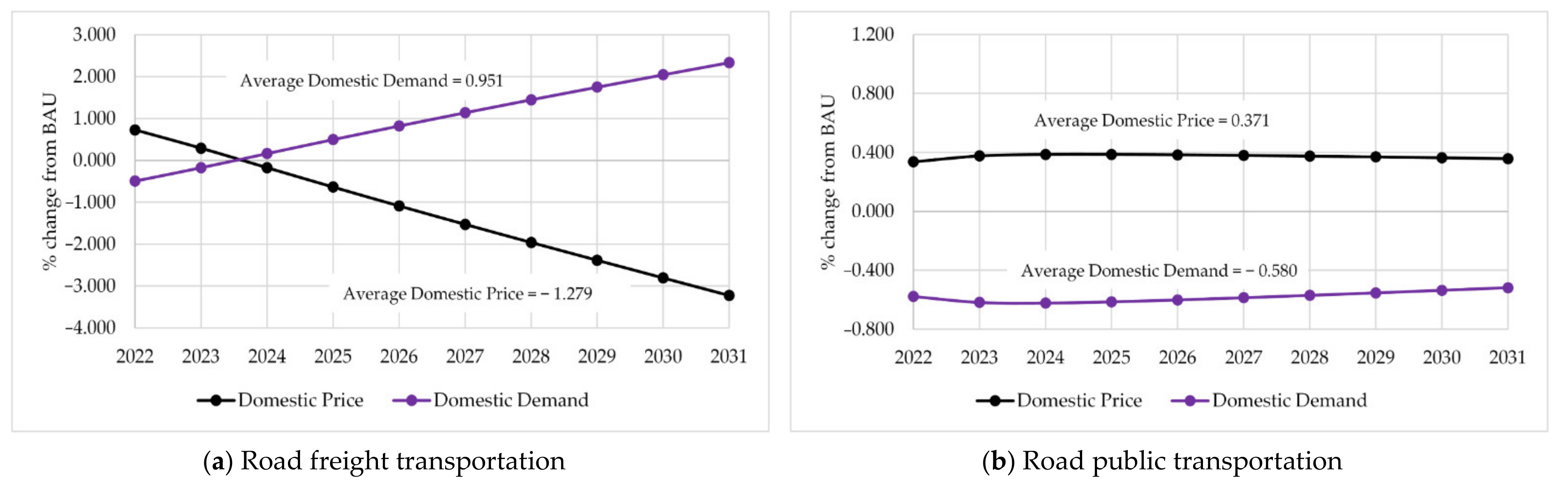
4.2.2. SIM B: Reallocating Biofuel Subsidy to Invest in Road Freight Transportation Sector

In this case, 50% of the terminated biofuel subsidy is reallocated to invest in road freight transportation. The changes in road transportation are shown in Figure 4. The results show no change in the price or demand for road public transportation. On the contrary, reallocation leads to changes in the price and demand for road freight transportation.

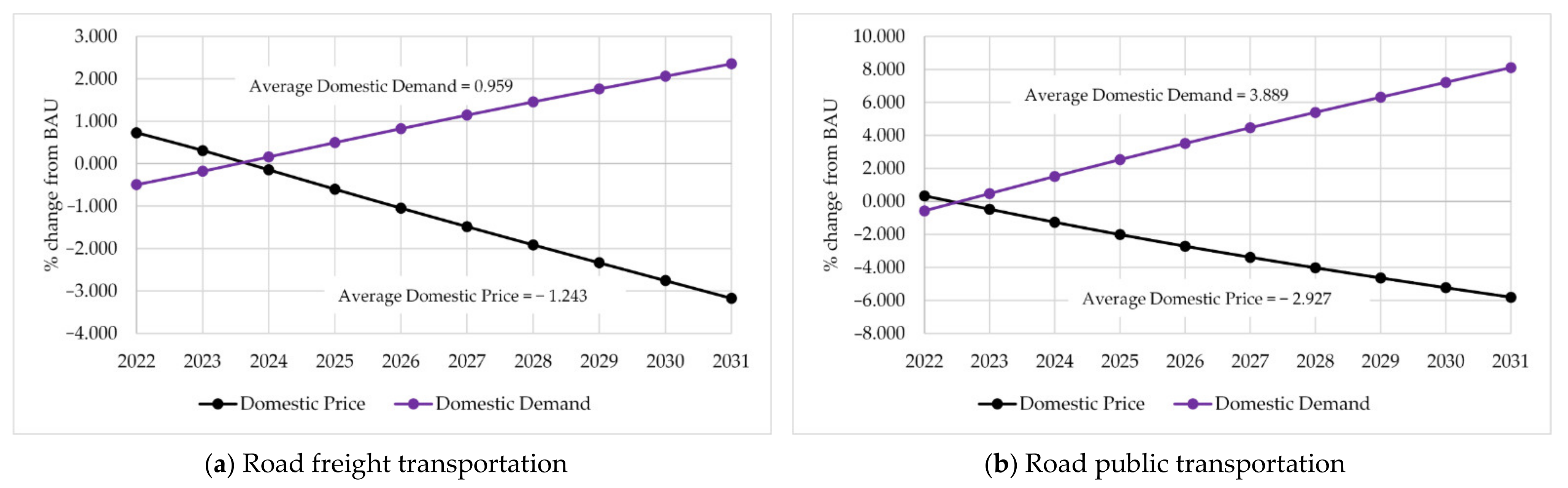
4.2.3. SIM C: Reallocating Biofuel Subsidy to Invest in Road Public Transportation Sector

Figure 5 shows the change in prices and demand for road transportation sectors when 50% of the terminated biofuel subsidy is invested in road public transportation. The prices of road public transportation decrease, but the demand increases. Moreover, investment in the road public transportation sector results in a greater change compared to investing in the road freight transport sector. This is because the costs associated with the road public transportation sector are significantly higher than those of the road freight transport sector. Therefore, it leads to a reduction in price and a rise in demand for the road freight transport sector.

In sum, although eliminating biofuel subsidy can increase the higher saving and rising government investment, the subsidy removal brings about the higher cost of productions that result in increasing inflation. However, reallocating the budgets to invest in road transportation can increase capital supply. Hence, the transportation facilities will be expanded, subsequently lowering the transportation cost and the economy-wide price level. With this change, the production costs of other sectors will continuously decrease as well. Thus, the investment mechanisms mitigate the adverse effects caused by biofuel subsidy removal.

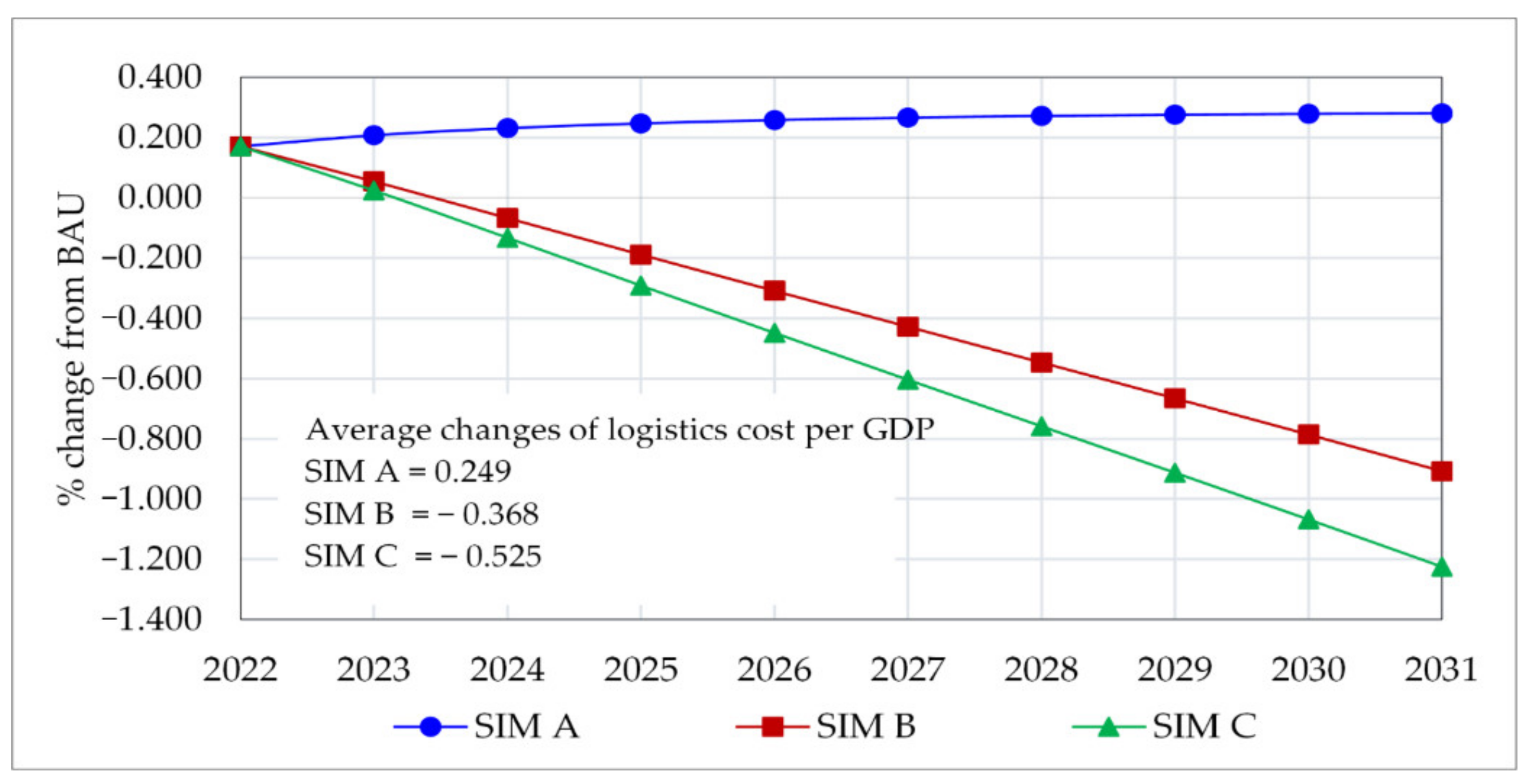
4.3. Change in Logistics Costs

Figure 6 shows that eliminating the biofuel subsidy (SIM A) leads to a minor increase in logistics costs per GDP (0.249%). In contrast, reallocating the biofuel subsidy to invest in public road transportation (SIM C) and road freight transportation (SIM B) leads to a decrease in logistics costs per GDP of 0.525% and 0.368%, respectively. It can be observed that SIM B and SIM C tend to continuously reduce logistics costs per GDP because of the higher demand and lower prices of road transportation sectors, as discussed in Section 4.2. Hence, the logistics costs per GDP and transportation costs both decrease.

4.4. Change in Macroeconomics

4.4.1. Consumer Price Index (CPI)

Figure 7 shows the effects of all scenarios on the CPI. The removal of the biofuel subsidy (SIM A) increases the CPI slightly (by 0.100% on average). In addition, it is likely to remain constant throughout the 10-year study period. Since investments play a role in road transportation sectors, the CPI changes are evident. Reallocating the budget to road freight transportation (SIM B) still increases the CPI by 0.062% on average. However, when the budget is reallocated to road public transportation (SIM C), the CPI decreases by 0.041% on average. The negative slope in SIM C is distinctly different from those in SIM A and SIM B. This is because, in SIM C, the prices of road freight and road public transportation decrease, as mentioned in Section 4.2.3, while in SIM B, only the price of road freight transportation decreases, as mentioned in Section 4.2.2. Therefore, reducing transportation prices leads to a decrease in production costs. This cost reduction is similar to that of a previous study [44], indicating that a reduced transport margin eventually decreases the CPI. This results in a greater decrease in the CPI in SIM C compared to SIM B.

4.4.2. Real Gross Domestic Product (Real GDP)

Figure 8 displays the impacts of biofuel subsidy removal and budget reallocation on real GDP. The results show that removing biofuel subsidies (SIM A) can reduce the average change in real GDP by 0.106%, and the trend slightly increases over the 10-year period. Conversely, reallocating the budget to invest in road freight transportation (SIM B) still decreases the average change in real GDP by 0.055%. In SIM C, in which the budget is reallocated to invest in public road transportation, the average change in real GDP increases by 0.049%.

The removal of the biofuel subsidy (SIM A) is the cause of an economic recession. However, investments in both transportation sectors (road freight and road public transportation) lead to economic recovery. Investment in the road freight transport sector can lead to a positive rebound of the real GDP after 2029, while investment in the road public transportation sector can lead to a positive enhancement of real GDP after 2025. The reasons are demonstrated by the price changes in the transportation sectors in Section 4.2.2 and Section 4.2.3. The reduction in prices of road freight and road public transportation leads to a decrease in production costs, contributing to overall productivity. Furthermore, the lower CPI can increase real GDP. Therefore, the investment measure in road transportation can compensate for the effects of biofuel subsidy removal.

4.4.3. Real Private Consumption (Real PCON)

Figure 9 presents the results of canceling the biofuel subsidy and reallocating it to invest in two types of road transportation. All scenarios result in a decrease in real PCON. SIM A, SIM B, and SIM C decrease real PCON by 0.302%, 0.263%, and 0.177%, respectively.

In SIM A, when the biofuel subsidy is eliminated, the prices of goods and services increase. Then, the outputs also decrease. Consequently, the revenue of labor and capital is reduced accordingly, which causes the household income to decrease as well. Due to the decrease in household incomes and the increase in commodity prices, eventually, real PCON decreases. In this scenario, there is no measure to mitigate the impacts; therefore, the change in real PCON is relatively constant for 10 years.

In SIM B, reallocation of the biofuel subsidy to invest in road freight transportation can mitigate the adverse effects of subsidy cancellation on real PCON. Although the average real PCON remains negative, the trend shows an upward change. This is because investment in the road freight transport sector directly decreases the prices of such transportation, as mentioned in Section 4.2.2. When the prices of road freight transportation decrease, the prices of all commodities are reduced as well. Thus, real PCON is higher in SIM B than in SIM A. However, the reallocation in SIM B cannot compensate for all of the effects, so the average real PCON remains negative.

In SIM C, reallocation of the biofuel subsidy to invest in road public transportation raises real PCON. Additionally, it is likely to be positive in the future (the slope is different). For the same reason as in SIM B, investment induces a price reduction in road public transportation, as mentioned in Section 4.2.3. Due to the two impacts, real PCON is higher in SIM C than in SIM B.

4.4.4. Real Gross Fixed Capital Formation (Real GFCF)

Figure 10 shows the impacts on real GFCF. All scenarios have positive average changes in real GFCF. Real GFCF increases by 0.213%, 0.321%, and 0.311% in SIM A, SIM B, and SIM C, respectively.

In SIM A, real GFCF initially increases because the biofuel subsidy is terminated, and the government receives more income for expenditures. However, the trend of real GFCF change decreases after 2025. This is because of the increase in the CPI, which increases the price index of investments. SIM A is different from SIM B and SIM C, in which real GFCF increases consecutively. Moreover, real GFCF is slightly higher in SIM B than in SIM C. This is because investment in road freight transportation increases the outputs of production sectors (i.e., agriculture-fishery and forestry, metal and non-metal, chemical production, rubber, and plastic production, electrical machinery production, transport industry, other manufacturing, construction, trading and services, road freight transportation (heavy), and road freight transportation (light) produce commodities for investments). These sectors have a high share of road freight transportation. Therefore, road freight transportation investment (SIM B) increases real GFCF to a greater extent than road public transportation investment (SIM C).

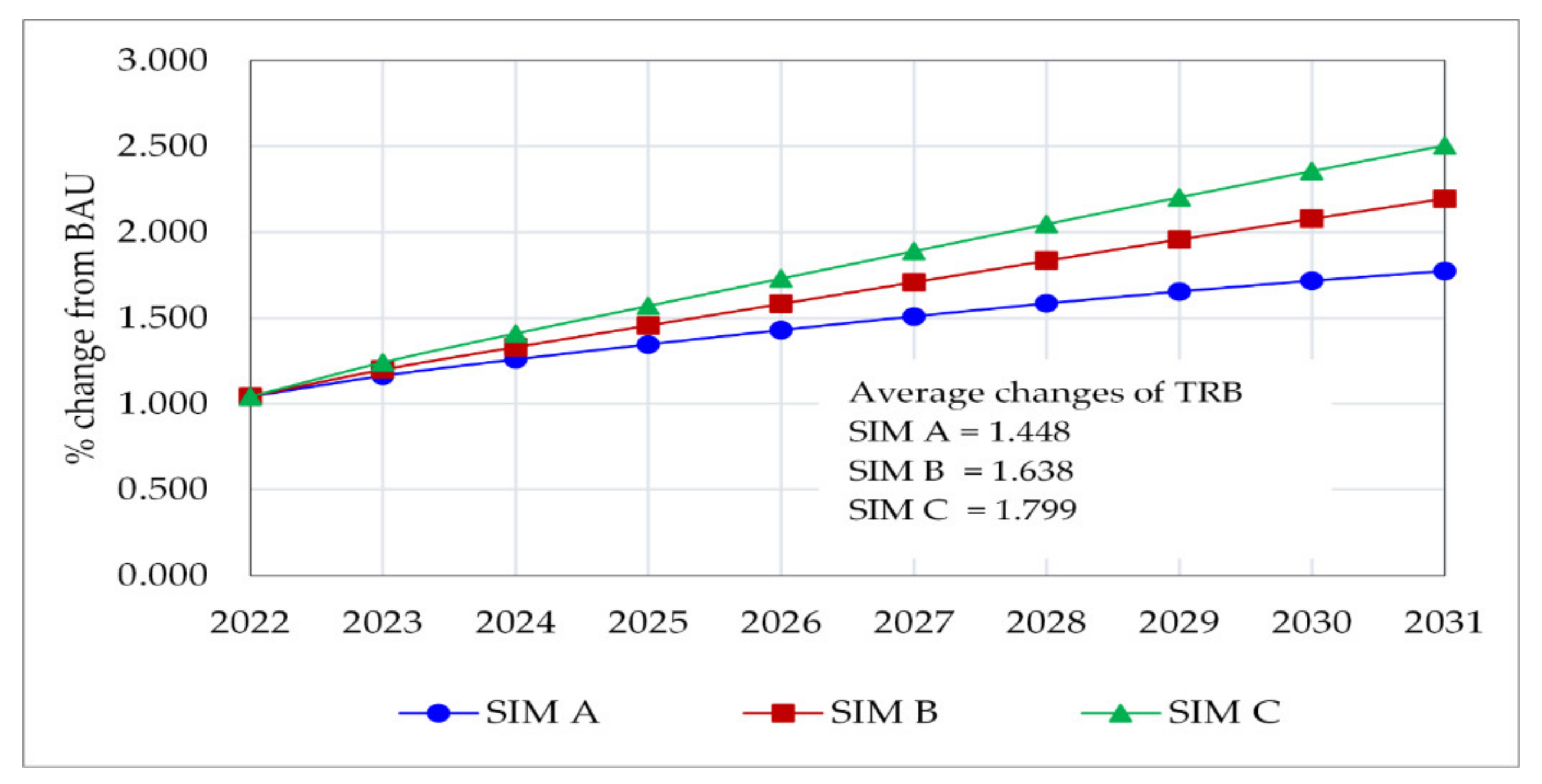
4.4.5. Trade Balance (TRB)

Figure 11 shows the impacts on TRB. TRB increases by 1.448%, 1.638%, and 1.799% in SIM A, SIM B, and SIM C, respectively. The removal of biofuel subsidy (SIM A) increases the government saving, which results in higher total investments. Moreover, in the cases of SIM B and C, an expansion of transportation investment can continuously lower the transportation cost and subsequently enhance Thailand’s export price competitive advantage. Therefore, the export will increase, leading to a continually higher trade surplus.

4.5. Sectoral Impacts

The recursive dynamic CGE model used in this study represents the main mechanism of Thailand’s economy, allowing economy-wide price endogenous adjustment. Hence, in addition to macroeconomic indicators, the model simulation results show the adjustment of prices and quantities of all production sectors, enabling a thorough investigation of positive and negative impacts. As exhibited in Table 3, in SIM A, the removal of the biofuel subsidy can directly reduce the production of ethanol (cassava-based), coastal and water transportation, and public road transportation. In addition, this contraction can indirectly lower the outputs of petroleum refinery and biodiesel production. On the other hand, this change can also cause the substitution of prices and factors of production, allowing the outputs of manufacturing, construction, metal and non-metal, electrical machinery, and railway freight transportation to increase.

In SIM B, the obtained sectoral impacts indicate that the expansion of road infrastructure can directly induce the production of construction raw materials and activities related to construction. Furthermore, the impacts positively influence the spillovers on road freight transportation (heavy), road freight transportation (light), construction, rubber plastics and chemicals production, and manufacturing. Simultaneously, this expansion leads to the substitution of factors of production, subsequently reducing the production of ethanol (cassava-based), coastal and water transportation, petroleum refinery, biodiesel production, and public road transportation.

In SIM C, the investment in public transportation can considerably expand both road freight transportation (heavy) and public road transportation. Additionally, the other sectors, i.e., land transportation services, road freight transportation (light), and transport industries can also increase due to the subsidy reallocation. On the contrary, the negative impacts on production and service activities are similar to those observed in SIM B, i.e., ethanol (cassava-based), coastal and water transportation, petroleum refinery, biodiesel production, and water transportation services. Notably, an investment in road public transportation can not only improve productivity itself but also enhance the output of road freight transportation (heavy). The main reason is due to the price adjustment of the road freight transportation sector described in Section 4.2.3.

4.6. Sensitivity Analysis

Figure 12 illustrates the outcomes of the Monte Carlo simulation for SIM A, B, and C. Similar to a previous study [45], the threshold of two standard deviations (2SD) identifies the highly probable range of simulation outcomes (with 95% probability). For SIM A—SIM C, the bands of 2SD of real GDP and real private consumption are stable, whereas those of the CPI and real gross fixed capital formation are tapering. Nevertheless, all sensitivity analysis outcomes show that the 95% probability range includes the opposite sign of the result. Therefore, the stability of substitution coefficients is very crucial. In practical implementation, the impact analysis should be constantly updated with the latest values of substitution coefficients.

4.7. Discussion

The main findings of simulation results can be classified into two categories.

(1): The adjustment mechanism of biofuel subsidy removal

Because the biofuel subsidy is a demand intervention policy, the results of SIM A represent the outcomes of removing the price distortion scheme. Hence, this change shifted the economy towards a new equilibrium with the market-based biofuel price. In accordance with previous studies [10,11,12,46,47,48], the rising biofuel price imposed burdens on many activities, subsequently inducing higher inflation and negative impacts on most activities. In addition, this negative effect has dynamic impacts on investment, which dampens the long-run capital accumulation (similar to the main findings of previous publications [12,49]). Hence, the economy will experience both short-term and long-term downturns.

(2): The integrated responses of subsidy removal and transportation investment

SIM B and SIM C exemplify the implementation of alternative policies that offset the negative impacts of biofuel subsidy removal. With the reallocated budget financing the transportation investment, this government-led supply-side stimulus can counteract the adverse effects and simultaneously induce gains in production and service activities. Similar to previous literature [15,19,25,26,27,28], the results of this study show that investment-led expansion can directly influence activities related to construction and machinery purchases. Thus, production outputs and employment in these sectors will benefit and subsequently create economy-wide positive spillovers. Furthermore, the continuously increasing investment will yield cumulative long-term benefits from the higher rate of capital accumulation. This change will permanently increase the capital stock in road transportation (i.e., facilities and machinery), consequently extending the capacity and coverage of this mode of transportation activity. Therefore, in accordance with many studies [8,9,21,22,23], the obtained simulation outcomes suggest that the road transportation investment is the preferred policy option.

4.8. Limitations and Further Study

The limitations of this study can be categorized into three issues that require further study. First, infrastructure investment should be extended to include other modes of transportation in the simulation analysis. Second, the specification of intertemporal relationships should be modified to embed the fully dynamic mechanism, enabling the foresight-based optimization of the economic agent. Third, the model should be enhanced to optimize the combination of sources of funds for financing the infrastructure investment, which will suggest additional valuable recommendations for policy implications.

5. Conclusions

This study examined the economy-wide impacts of reallocating the biofuel subsidy to finance road transportation investment. A recursive dynamic CGE model was constructed based on the official input–output table, which was subsequently extended to SAM. The model was validated with the actual 2015–2019 data and showed a low percentage of discrepancies, ranging from 1.33 to 7.22%. The simulation result revealed that terminating the biofuel subsidy can cause negative impacts on the economy, whereas reallocating this amount to finance investment in road transportation can offset the impacts and eventually lead to positive outcomes. In addition, the simulation result showed that investing in road public transportation can generate greater impacts than investing in road freight transportation. All findings suggest that an investment in transportation infrastructure yields higher long-term gains than the short-term price distortion scheme. Therefore, policymakers should maintain transportation investment as their top priority based on its long-term economy-wide benefits. In addition, this policy suggestion would be a guideline for other developing countries seeking the alternative scheme for offsetting the adverse consequences of fuel subsidy removal.

Author Contributions

Conceptualization, K.P., N.P. and M.P.; data curation, K.P.; formal analysis, K.P.; funding acquisition, M.P.; investigation, K.P. and N.P.; methodology, K.P. and N.P.; project administration, N.P. and M.P.; resource, K.P. and N.P.; software, N.P. and M.P.; supervision, N.P. and M.P.; validation, K.P., N.P. and M.P.; visualization, K.P. and N.P.; writing—original draft preparation, K.P.; writing—review and editing, N.P. and M.P. All authors have read and agreed to the published version of the manuscript.

Funding

This research was funded by the Joint Graduate School of Energy and Environment (JGSEE) and the Sirindhorn International Institute of Technology (SIIT).

Institutional Review Board Statement

Not applicable.

Informed Consent Statement

Not applicable.

Data Availability Statement

Not applicable.

Conflicts of Interest

The authors declare no conflict of interest. The funders had no role in the design of the study; in the collection, analyses, or interpretation of data; in the writing of the manuscript, or in the decision to publish the results.

Appendix A

Table A1. Sectors and commodities in the CGE model.

Sector Number	Industries	IO Code	Commodity Number	Commodities
1	Agriculture forest and fishery	001–003, 005–008, 010, 012–029	1	Agriculture forest and fishery
2	Cassava plantation	004	2	Cassava
3	Sugarcane plantation	009	3	Sugarcane
4	Oil palm plantation	011	4	Oil palm
5	Food industry	042–054, 056–066	5	Food products
6	Crude palm oil production	047	6	Crude palm oil
7	Sugar refinery	055	7	Sugar products
			8	Molasses
8	Coal and lignite mining	030	9	Coal and lignite
9	Crude oil and natural gas	031	10	Crude oil and natural gas
10	Other mining	032–041	11	Other mineral products
11	Petroleum refinery	093–094	12	Liquefied petroleum gas
			13	Jet and kerosene
			14	Fuel oil
			15	Other petroleum products
			16	Gasohol E10 and gasoline
			17	Gasohol E20 and E85
			18	Biodiesel B5/7 (mandatory)
			19	Biodiesel B10/B20 (option)
12	Biodiesel production	093	20	Purified biodiesel (B100)
13	Ethanol (cassava-based)	093	21	Ethanol
14	Ethanol (molasses-based)	093
15	Electricity production	135	22	Electricity
16	Natural gas separation	136	23	Natural gas products
17	Metal and non-metal	110–111	24	Metal and non-metal
18	Chemical production	067–092	25	Chemical products
19	Rubber and plastic production	095–109	26	Rubber, plastics, and material
20	Electrical machinery production	112–122	27	Electrical machinery and equipment
21	Transport industry	123–128	28	Transport machinery and maintenance
22	Other manufacturing	129–134	29	Other industrial products
23	Construction	137–144	30	Construction
24	Trading and services	145–148, 160–164	31	Trading and services
25	Public administration	165–171	32	Public administration
26	Railway freight transportation	149	33	Railway freight transportation
27	Railway mass transportation	149	34	Railway mass transportation
28	Road public transportation	150	35	Road public transportation
29	Road freight transportation (heavy)	151	36	Road freight transportation (heavy)
30	Road freight transportation (light)	151	37	Road freight transportation (light)
31	Land transportation services	152	38	Land transportation services
32	Ocean and coastal transportation	153–154	39	Ocean and coastal transportation
33	Water transportation services	155	40	Water transportation services
34	Air transportation	156	41	Air transportation
35	Other services and activities	157–159, 172–180	42	Other services and activities

Table A2. Coefficients of elasticity of substitution.

Sector Number	Industries	Coefficients of Elasticity of Substitution
Sector Number	Industries	[a]	[b]	[c]	[d]	[e]
1	Agriculture forest and fishery	1.15	0.5	0.5	0.5	0.5
2	Cassava plantation	1.15	0.5	0.5	0.5	0.5
3	Sugarcane plantation	1.15	0.5	0.5	0.5	0.5
4	Oil palm plantation	1.15	0.5	0.5	0.5	0.5
5	Food industry	0.86	0.5	0.5	0.5	0.5
6	Crude palm oil production	0.86	0.5	0.5	0.5	0.5
7	Sugar refinery	0.86	0.5	0.5	0.5	0.5
8	Coal and lignite mining	1.1	0.5	0.5	0.5	0.5
9	Crude oil and natural gas	1.1	0.5	0.5	0.5	0.5
10	Other mining	1.1	0.5	0.5	0.5	0.5
11	Petroleum refinery	1.1	0.5	0.5	0.5	0.5
12	Biodiesel production	1.1	0.5	0.5	0.5	0.5
13	Ethanol (cassava based)	0.86	0.5	0.5	0.5	0.5
14	Ethanol (molasses based)	0.86	0.5	0.5	0.5	0.5
15	Electricity production	1.02	0.5	0.5	0.5	0.5
16	Natural gas separation	1.02	0.5	0.5	0.5	0.5
17	Metal and non-metal	0.86	0.5	0.5	0.5	0.5
18	Chemical production	0.86	0.5	0.5	0.5	0.5
19	Rubber and plastic production	0.86	0.5	0.5	0.5	0.5
20	Electrical machinery production	0.86	0.5	0.5	0.5	0.5
21	Transport industry	0.87	0.5	0.5	0.5	0.5
22	Other manufacturing	0.86	0.5	0.5	0.5	0.5
23	Construction	0.97	0.5	0.5	0.5	0.5
24	Trading and services	0.87	0.5	0.5	0.5	0.5
25	Public administration	1.04	0.5	0.5	0.5	0.5
26	Railway freight transportation	1.03	0.5	0.5	0.5	0.5
27	Railway mass transportation	1.03	0.5	0.5	0.5	0.5
28	Road public transportation	1.03	0.5	0.5	0.5	0.5
29	Road freight transportation (heavy)	1.03	0.5	0.5	0.5	0.5
30	Road freight transportation (light)	1.03	0.5	0.5	0.5	0.5
31	Land transportation services	1.03	0.5	0.5	0.5	0.5
32	Ocean and coastal transportation	1.03	0.5	0.5	0.5	0.5
33	Water transportation services	1.03	0.5	0.5	0.5	0.5
34	Air transportation	1.03	0.5	0.5	0.5	0.5
35	Other services and activities	1.03	0.5	0.5	0.5	0.5

Notes: [a] is elasticity of substitution between labor and capital based on [37]; [b] is elasticity of substitution between biodiesel (B5/B7 vs. B10); [c] is elasticity of substitution between gasoline/gasohol E10 vs. gasohol E20/E85; [d] is elasticity of substitution between road freight transportation and railway freight transportation; [e] is elasticity of substitution between road public transportation and railway passenger transportation; [b], [c], [d], and [e] are based on the assumption of the authors. The other types of elasticity, i.e., the elasticity of transformation between products of industry j = 2, the elasticity of transformation between exports and local supplies of commodity i by industry j = 2, and the elasticity of substitution between imported and domestically produced commodity i = 2 are based on [30].

Table A3. Dynamic parameters.

Year	n	eg	ig	itg	etr	ppg	δ	γ
2019–2031	0.01	0.05	0.05	0.055	0.05	0.01	0.07	2

Notes: n = population growth [50]; eg = government expenditures growth [33]; ig = public sector investment growth [33]; itg = total investment growth [33]; etr = export growth [33]; ppg = total factor productivity growth [34]; δ = depreciation rate [32,37]; γ = elasticity of investment demand [32,37].

Appendix B

Lists of sets, parameters, variables, and equations of CGE model.

Appendix B.1. Set

The subscripts in equations are a set of economic agents shown in Table A1 in Appendix A.

j	All sectors
pub	Public sectors (sector number 25–30)
pri	Private industries (sector number 1–24 and 31–35)
j0	All sectors except sector number 7 and 11
j1	Sugar and petroleum refinery sector (sector number 7 and 11)
i	All commodities
ij	All commodities (alias commodities)
i1	All commodities except sector number 16–19 and 33–36
i2	Mixed gasohol (sector number 16, 17)
i3	Mixed biodiesel (sector number 18, 19)
i4	Mass transportation (sector number 34, 35)
i5	Freight transportation (sector number 33, 36)
l	Labor
k	Capital
ag	All agents (firms, households, government, and the rest of the world)
agng	Non-government agents (firms, households, and the rest of the world)
agd	Domestic agents (firms, households, and government)
gvt	Government
row	The rest of the world
f	Firms
h	Households
t	Time for simulation

Appendix B.2. Parameters

Appendix B.2.1. Input-Output Co-Efficient

$a i j_{i, j}$	Input-output coefficient of intermediate commodity i for industry j
$a d m_{j}$	Input-output coefficient of mixed biodiesel for industry j
$a g m_{j}$	Input-output coefficient of mixed gasohol for industry j
$a f t_{j}$	Input-output coefficient of freight transportation for industry j
$a m t_{j}$	Input-output coefficient of mass transportation for industry j
$i o_{j}$	Input-output coefficient (total intermediate consumption) for industry j
$v_{j}$	Input-output coefficient (total value added) for industry j

Appendix B.2.2. Scale Share and Elasticity of Production Function

$B_{j, t}^{V A T}$	Scale parameter (CES—value added) for industry j
$β_{j}^{V A}$	Share parameter (CES—value added) for industry j
$ρ_{j}^{V A}$	Elasticity parameter (CES—value added) for industry j; $- 1 < ρ_{j}^{V A} < \infty$
$σ_{j}^{V A}$	Elasticity of substitution (CES—value added) for industry j; $0 < σ_{j}^{V A} < \infty$ where $ρ_{j}^{V A} = \frac{1 - σ_{j}^{V A}}{σ_{j}^{V A}}$
$B_{j}^{K D}$	Scale parameter (CES—composite capital) for industry j
$β_{k, j}^{K D}$	Share parameter (CES—composite capital) for industry j
$ρ_{j}^{K D}$	Elasticity parameter (CES—composite capital) for industry j; $- 1 < ρ_{j}^{K D} < \infty$
$σ_{j}^{K D}$	Elasticity of substitution (CES—composite capital) for industry j; $0 < σ_{j}^{K D} < \infty$ where $ρ_{j}^{K D} = \frac{1 - σ_{j}^{K D}}{σ_{j}^{K D}}$
$B_{j}^{L D}$	Scale parameter (CES—composite labor) for industry j
$β_{l, j}^{L D}$	Share parameter (CES—composite labor) for industry j
$ρ_{j}^{L D}$	Elasticity parameter (CES—composite labor) for industry j; $- 1 < ρ_{j}^{L D} < \infty$
$σ_{j}^{L D}$	Elasticity of substitution (CES—composite labor) for industry j; $0 < σ_{j}^{L D} < \infty$ where $ρ_{j}^{L D} = \frac{1 - σ_{j}^{L D}}{σ_{j}^{L D}}$
$B_{j}^{G M}$	Scale parameter (CES—composite mixed gasohol) for industry j
$β_{j}^{G M}$	Share parameter (CES—composite mixed gasohol) for industry j
$ρ_{j}^{G M}$	Elasticity parameter (CES—mixed gasohol) for industry j; $- 1 < ρ_{j}^{G M} < \infty$
$σ_{j}^{G M}$	Elasticity of substitution (CES—mixed gasohol) for industry j; $0 < σ_{j}^{G M} < \infty$ where $ρ_{j}^{G M} = \frac{1 - σ_{j}^{G M}}{σ_{j}^{G M}}$
$B_{j}^{D M}$	Scale parameter (CES—composite mixed biodiesel) for industry j
$β_{j}^{D M}$	Share parameter (CES—composite mixed biodiesel) for industry j
$ρ_{j}^{D M}$	Elasticity parameter (CES—mixed biodiesel) for industry j; $- 1 < ρ_{j}^{D M} < \infty$
$σ_{j}^{D M}$	Elasticity of substitution (CES—mixed biodiesel) for industry j; $0 < σ_{j}^{D M} < \infty$ where $ρ_{j}^{D M} = \frac{1 - σ_{j}^{D M}}{σ_{j}^{D M}}$
$B_{j}^{M T}$	Scale parameter (CES—mass transportation) for industry j
$β_{j}^{M T}$	Share parameter (CES—mass transportation) for industry j
$ρ_{j}^{M T}$	Elasticity parameter (CES—mass transportation) for industry j; $- 1 < ρ_{j}^{M T} < \infty$
$σ_{j}^{M T}$	Elasticity of substitution (CES—mass transportation) for industry j; $0 < σ_{j}^{M T} < \infty$ where $ρ_{j}^{M T} = \frac{1 - σ_{j}^{M T}}{σ_{j}^{M T}}$
$B_{j}^{F T}$	Scale parameter (CES—freight transportation) for industry j
$β_{j}^{F T}$	Share parameter (CES—freight transportation) for industry j
$ρ_{j}^{F T}$	Elasticity parameter (CES—freight transportation) for industry j; $- 1 < ρ_{j}^{F T} < \infty$
$σ_{j}^{F T}$	Elasticity of substitution (CES—freight transportation) for industry j; $0 < σ_{j}^{F T} < \infty$ where $ρ_{j}^{F T} = \frac{1 - σ_{j}^{F T}}{σ_{j}^{F T}}$
$B_{i}^{M}$	Scale parameter (CES—composite commodity)
$β_{i}^{M}$	Share parameter (CES—composite commodity)
$ρ_{i}^{M}$	Elasticity parameter (CES—composite commodity); $- 1 < ρ_{i}^{M} < \infty$
$σ_{i}^{M}$	Elasticity of substitution (CES—composite commodity); $0 < σ_{i}^{M} < \infty$ where $ρ_{i}^{M} = \frac{1 - σ_{i}^{M}}{σ_{i}^{M}}$
$B_{j, i}^{X}$	Scale parameter (CET—exports and local sales)
$β_{j, i}^{X}$	Share parameter (CET—exports and local sales)
$ρ_{j, i}^{X}$	Elasticity parameter (CET—exports and local sales); $1 < ρ_{j, i}^{X} < \infty$
$σ_{j, i}^{X}$	Elasticity of transformation (CET—total output); $0 < σ_{j}^{X T} < \infty$ where $ρ_{j, i}^{X} = \frac{1 + σ_{j, i}^{X}}{σ_{j, i}^{X}}$
$B_{j}^{X T}$	Scale parameter (CET—total output) for industry j
$β_{j, i}^{X T}$	Share parameter (CET—total output) for industry j
$ρ_{j}^{X T}$	Elasticity parameter (CET—total output) for industry j; $1 < ρ_{j}^{X T} < \infty$
$σ_{j}^{X T}$	Elasticity of transformation (CET—total output) for industry j; $0 < σ_{j}^{X T} < \infty$ where $ρ_{j}^{X T} = \frac{1 + σ_{j}^{X T}}{σ_{j}^{X T}}$
$σ_{i}^{X D}$	Price-elasticity of the world demand for exports of product i
$e x t r_{i, t}$	Export growth rate of product i

Appendix B.2.3. Parameters for Income Saving and Investment of Institutes

$λ_{a g, k}^{R K}$	Share of type k capital income received by agent ag
$λ_{h, l}^{W L}$	Share of type l labor income received by type h households
$s h 0_{h, t}$	Intercept (type h household savings)
$s h 1_{h, t}$	Slope (type h household savings)
$γ_{i, h}^{L E S}$	Marginal share of commodity i in type h household consumption budget
$γ_{i}^{I N V P R I}$	Share of commodity i in total private investment expenditures
$γ_{i}^{I N V P U B}$	Share of commodity i in total public investment expenditures
$γ_{i}^{G V T}$	Share of commodity i in total current public expenditures on goods and services
$A^{K_P R I}$	Scale parameter (price for new private capital)
$A^{K_P U B}$	Scale parameter (price for new public capital)
$ϕ_{k, p r i}$	Scale parameter (allocation of investment to industry)
$δ_{k, p u b}$	Deprecation rate of capital k used in public

Appendix B.2.4. Tax and Transfer

$λ_{a g, a g}^{T R}$	Share parameter (transfer functions) between ag
$η$	Price elasticity of indexed transfers and parameters
$t m r g_{i, i}$	Rate of transport margin applied to domestic commodity i
$t m r g_{i, i}^{X}$	Rate of transport margin applied to export commodity i
$t r 0_{g v t, h, t}$	Intercept (transfers by type h households to government)
$t r 1_{g v t, h, t}$	Marginal rate of transfers by type h households to government
$t t i c_{i, t}$	Tax rate on commodity i
$t t d f 0_{f, t}$	Intercept (income taxes of type f businesses)
$t t d f 1_{f, t}$	Marginal income tax rate of type f businesses
$t t d h 0_{h, t}$	Intercept (income taxes of type h households)
$t t d h 1_{h, t}$	Marginal income tax rate of type h households
$t t i k_{k, j, t}$	Tax rate on type k capital used by industry j
$t t i m_{i, t}$	Rate of taxes and duties on imports of commodity i
$t t i p_{j, t}$	Tax rate on the production of industry j
$t t i w_{l, j, t}$	Tax rate on type l worker compensation in industry j
$t t i x_{i, t}$	Export tax rate on exported commodity i

Appendix B.3. Variables

Appendix B.3.1. Prices and Wages

$P_{j, i, t}$	Basic price of industry j’s production of commodity i
$P C_{i, t}$	Purchaser price of composite commodity i (including all taxes and margins)
$P C_{i}^{0}$	Purchaser price of composite commodity i (base year)
$P C I_{j, t}$	Intermediate consumption price index of industry j
$P D_{i, t}$	Price of local product i sold on the domestic market
$P D M_{j, t}$	Aggregate price of mixed biodiesel by industry j
$P E_{i, t}$	Price received for exported commodity i (excluding export taxes)
$P E_{i, t}^{F O B}$	FOB price of exported commodity i (in local currency)
$P F T_{j, t}$	Aggregate price of freight transportation by industry j
$P G M_{j, t}$	Aggregate price of mixed gasohol by industry j
$P I X C O N_{t}^{η}$	Consumer price index
$P I X G D P_{t}$	GDP deflator
$P I X G V T_{t}$	Public expenditures price index
$P I X I N V_{t}^{P R I}$	Private Investment price index
$P I X I N V_{t}^{P U B}$	Public Investment price index
$P K_{t}^{P R I}$	Price of new private capital
$P K_{t}^{P U B}$	Price of new public capital
$P L_{i, t}$	Price of local product i (excluding all taxes on products)
$P M_{i, t}$	Price of imported product i (including all taxes and margins)
$P M T_{j, t}$	Aggregate price of mass transportation by industry j
$P P_{j, t}$	Industry j unit cost
$P T_{j, t}$	Basic price of industry j output
$P V A_{j, t}$	Price of industry j value added
$P W M_{i, t}$	World price of imported product i (expressed in foreign currency)
$P W X_{i, t}$	World price of exported product i (expressed in foreign currency)
$R_{k, j, t}$	Rental rate of type k capital in industry j
$R C_{j, t}$	Rental rate of industry j composite capital
$R T I_{k, j, t}$	Rental rate paid by industry j for type k capital, including capital taxes
$W_{l, t}$	Wage rate of type l labor
$W C_{j, t}$	Wage rate of industry j composite labor
$W T I_{l, j, t}$	Wage rate paid by industry j for type l labor, including payroll taxes
$U_{k, p r i, t}$	User cost of type k capital in private industry
$U_{k, p u b, t}$	User cost of type k capital in public industry

Appendix B.3.2. Taxes

$T D F_{f, t}$	Income taxes of type f businesses
$T D F T_{t}$	Total government revenue from business income taxes
$T D H_{h, t}$	Income taxes of type h households
$T D H T_{t}$	Total government revenue from household income taxes
$T I C_{i, t}$	Government revenue from indirect taxes on product i
$T I C T_{t}$	Total government receipts of indirect taxes on commodities
$T I K_{k, j, t}$	Government revenue from taxes on type k capital used by industry j
$T I K T_{t}$	Total government revenue from taxes on capital
$T I M_{i, t}$	Government revenue from import duties on product i
$T I M T_{t}$	Total government revenue from import duties
$T I P_{j, t}$	Government revenue from taxes on industry j production (excluding taxes directly related to the use of capital and labor)
$T I P T_{t}$	Total government revenue from production taxes (excluding taxes directly related to the use of capital and labor)
$T I W_{l, j, t}$	Government revenue from payroll taxes on type l labor in industry j
$T I W T_{t}$	Total government revenue from payroll taxes
$T I X_{i, t}$	Government revenue from export taxes on product i
$T I X T_{t}$	Total government revenue from export taxes

Appendix B.3.3. Quantity

$C_{i, h, t}$	Consumption of commodity i by type h households
$C_{i, h, t}^{M I N}$	Minimum consumption of commodity i by type h households
$C G_{i, t}$	Public consumption of commodity i (volume)
$C I_{j, t}$	Total intermediate consumption of industry j
$C T H_{h, t}$	Consumption budget of type h households
$C T H_{h, t}^{R E A L}$	Real consumption expenditure of households h
$D D_{i, t}$	Domestic demand for commodity i produced locally
$D I_{i, j, t}$	Intermediate consumption of commodity i by industry j
$D I D M_{j, t}$	Aggregate intermediate consumption of mixed biodiesel by industry j
$D I F T_{j, t}$	Aggregate intermediate consumption of freight transportation by industry j
$D I G M_{j, t}$	Aggregate intermediate consumption of mixed gasohol by industry j
$D I M T_{j, t}$	Aggregate intermediate consumption of mass transportation by industry j
$D I T_{i, t}$	Total intermediate demand for commodity i
$D S_{j, i, t}$	Supply of commodity i by sector j to the domestic market
$E X_{j, i, t}$	Quantity of product i exported by sector j
$E X D_{i, t}$	World demand for exports of product i
$E X D_{i}$	World demand for exports of product i (base year)
$I M_{i, t}$	Quantity of product i imported
$I N D_{k, j, t}$	Volume of new type k capital investment to sector j
$I N V_{i, t}$	Final demand of commodity i for investment purposes
$I N V_{i, t}^{P R I}$	Final demand of commodity i for private investment purposes
$I N V_{i, t}^{P U B}$	Final demand of commodity i for public investment purposes
$K D_{k, j, t}$	Demand for type k capital by industry j
$K D C_{j, t}$	Industry j demand for composite capital
$K S_{k, t}$	Supply of type k capital
$L D_{l, j, t}$	Demand for type l labor by industry j
$L D C_{j, t}$	Industry j demand for composite labor
$L S_{l, t}$	Supply of type l labor
$M R G N_{i, t}$	Demand for commodity i as a trade or transport margin
$Q_{i, t}$	Quantity demanded of composite commodity i
$V A_{j, t}$	Value added of industry j
$V S T K_{i, t}$	Inventory change of commodity i
$X S_{j, i, t}$	Industry j production of commodity i
$X S T_{j, t}$	Total aggregate output of industry j

Appendix B.3.4. Value

$C A B_{t}$	Current account balance
$G_{t}$	Current government expenditures on goods and services
$G_{t}^{R E A L}$	Real government expenditures
$G D P_{t}^{B P_R E A L}$	Real GDP at basic price
$G D P_{t}^{M P_R E A L}$	Real GDP at market price
$G F C F_{t}^{P R I_R E A L}$	Real private gross fixed capital formation
$G F C F_{t}^{P U B_R E A L}$	Real public gross fixed capital formation
$G F C F_{t}$	Gross fixed capital formation
$G D P^{B P}$	GDP at basic prices
$G D P^{F D}$	GDP at purchasers’ prices from the perspective of final demand
$G D P^{I B}$	GDP at market prices (income-based)
$G D P^{M P}$	GDP at market prices
$I T_{t}$	Total investment expenditures
$I T_{t}^{P R I}$	Total private investment expenditures
$I T_{t}^{P U B}$	Total public investment expenditures
$R I N V_{k, j, t}$	Reallocation budget k for industry j
$S F_{f, t}$	Savings of type f businesses
$S G_{t}$	Government savings
$S R O W_{t}$	Rest-of-the-world savings
$S H_{h, t}$	Savings of type h households
$T R_{h, a g, t}$	Transfers from agent ag to type h households
$T P R C T S_{t}$	Total government revenue from taxes on products and imports
$T P R O D N_{t}$	Total government revenue from other taxes on production
$Y D F_{f, t}$	Disposable income of type f businesses
$Y D H_{h, t}$	Disposable income of type h households
$Y F_{f, t}$	Total income of type f businesses
$Y F K_{f, t}$	Capital income of type f businesses
$Y F T R_{f, t}$	Transfer income of type f businesses
$Y G_{t}$	Total government income
$Y G K_{t}$	Government capital income
$Y G T R_{t}$	Government transfer income
$Y H_{h, t}$	Total income of type h households
$Y H K_{h, t}$	Capital income of type h households
$Y H L_{h, t}$	Labor income of type h households
$Y H T R_{h, t}$	Transfer income of type h households
$Y R O W_{t}$	Rest-of-the-world income

Appendix B.3.5. Monetary

$e_{t}$	Exchange rate; price of foreign currency in terms of local currency
$I R_{t}$	Interest rate

Appendix B.4. Equation

V A_{j, t} = v_{j} X S T_{j, t}

(A1)

C I_{j, t} = i o_{j} X S T_{j, t}

(A2)

V A_{j, t} = B_{j}^{V A} {[β_{j}^{V A} L D C_{j, t}^{- ρ_{j}^{V A}} + (1 - β_{j}^{V A}) K D C_{j, t}^{- ρ_{j}^{V A}}]}^{- \frac{1}{ρ_{j}^{V A}}}

(A3)

L D C_{j, t} = {[\frac{β_{j}^{V A}}{1 - β_{j}^{V A}} \frac{R C_{j, t}}{W C_{j, t}}]}^{σ_{j}^{V A}} K D C_{j, t}

(A4)

L D C_{j, t} = B_{j}^{L D} {[\sum_{l} β_{l . j}^{L D} L D_{l . j, t}^{- ρ_{j}^{L D}}]}^{- \frac{1}{ρ_{j}^{L D}}}

(A5)

K D C_{j, t} = B_{j}^{K D} {[\sum_{k} β_{k . j}^{K D} K D_{k . j, t}^{- ρ_{j}^{K D}}]}^{- \frac{1}{ρ_{j}^{K D}}}

(A6)

L D_{l, j, t} = {[\frac{β_{l . j}^{L D} W C_{j, t}}{W T I_{l, j, t}}]}^{σ_{j}^{L D}} {(B_{j}^{L D})}^{σ_{j}^{L D} - 1} L D C_{j, t}

(A7)

K D_{k, j, t} = {[\frac{β_{k . j}^{K D} R C_{j, t}}{R T I_{k, j, t}}]}^{σ_{j}^{K D}} {(B_{j}^{K D})}^{σ_{j}^{K D} - 1} K D C_{j, t}

(A8)

D I_{i 1, j, t} = a i j_{i 1, j} C I_{j, t}

(A9)

D I G M_{j, t} = a g m_{j} C I_{j, t}

(A10)

D I D M_{j, t} = a d m_{j} C I_{j, t}

(A11)

D I M T_{j, t} = a m t_{j} C I_{j, t}

(A12)

D I F T_{j, t} = a f t_{j} C I_{j, t}

(A13)

D I G M_{j, t} = B_{j}^{G M} {[\sum_{i 2} β_{i 2, j}^{G M} D I_{i 2 . j, t}^{- ρ_{j}^{G M}}]}^{- \frac{1}{ρ_{j}^{G M}}}

(A14)

D I_{i 2, j, t} = {[\frac{β_{i 2 . j}^{G M} P G M_{j, t}}{P C_{i 2, t}}]}^{σ_{j 1}^{G M}} {(B_{j}^{G M})}^{σ_{j}^{G M} - 1} D I G M_{j, t}

(A15)

D I D M_{j, t} = B_{j}^{D M} {[\sum_{i 3} β_{i 3, j}^{D M} D I_{i 3, j, t}^{- ρ_{j}^{D M}}]}^{- \frac{1}{ρ_{j}^{D M}}}

(A16)

D I_{i 3, j, t} = {[\frac{β_{i 3 . j}^{D M} P D M_{j, t}}{P C_{i 3, t}}]}^{σ_{j}^{G M}} {(B_{j}^{D M})}^{σ_{j}^{D M} - 1} D I D M_{j, t}

(A17)

D I M T_{j, t} = B_{j}^{M T} {[\sum_{i 4} β_{i 4, j}^{M T} D I_{i 4, j, t}^{- ρ_{j}^{M T}}]}^{- \frac{1}{ρ_{j}^{M T}}}

(A18)

D I_{i 4, j, t} = {[\frac{β_{i 4 . j}^{M T} P M T_{j, t}}{P C_{i 4, t}}]}^{σ_{j}^{M T}} {(B_{j}^{M T})}^{σ_{j}^{M T} - 1} D I M T_{j, t}

(A19)

D I F T_{j, t} = B_{j}^{F T} {[\sum_{i 5} β_{i 5, j}^{F T} D I_{i 5, j, t}^{- ρ_{j}^{F T}}]}^{- \frac{1}{ρ_{j}^{F T}}}

(A20)

D I_{i 5, j, t} = {[\frac{β_{i 5 . j}^{F T} P F T_{j, t}}{P C_{i 5, t}}]}^{σ_{j}^{F T}} {(B_{j}^{F T})}^{σ_{j}^{F T} - 1} D I F T_{j, t}

(A21)

Y H_{h, t} = Y H L_{h, t} + Y H K_{h, t} + Y H T R_{h, t}

(A22)

Y H L_{h, t} = \sum_{l} λ_{h, l}^{W L} (W_{l, t} \sum_{j} L D_{l, j, t})

(A23)

Y H K_{h, t} = \sum_{k} λ_{h, k}^{R K} (\sum_{j} R_{k, j, t} K D_{k, j, t})

(A24)

Y H T R_{h, t} = \sum_{a g} T R_{h, a g, t}

(A25)

Y D H_{h, t} = Y H_{h, t} - T D H_{h, t} - T R_{g v t, h, t}

(A26)

C T H_{h, t} = Y D H_{h, t} - S H_{h, t} - \sum_{a g n g} T R_{a g n g, h, t}

(A27)

S H_{h, t} = P I X C O N_{t}^{η} s h 0_{h, t} + s h 1_{h, t} Y D H_{h, t}

(A28)

Y F_{f, t} = Y F K_{f, t} + Y F T R_{f, t}

(A29)

Y F K_{f, t} = \sum_{k} λ_{f, k}^{R K} (\sum_{j} R_{k, j, t} K D_{k, j, t})

(A30)

Y F T R_{f, t} = \sum_{a g} T R_{f, a g, t}

(A31)

S F_{f, t} = Y D F_{f, t} - \sum_{a g} T R_{a g, f, t}

(A32)

Y D F_{f, t} = Y F_{f, t} - T D F_{f, t}

(A33)

Y G_{t} = Y G K_{t} + T D H T_{t} + T D F T_{t} + T P R O D N_{t} + T P R C T S_{t} + Y G T R_{t}

(A34)

Y G K_{t} = \sum_{k} λ_{g v t, k}^{R K} (\sum_{j} R_{k, j, t} K D_{k, j, t})

(A35)

T D H T_{t} = \sum_{h} T D H_{h, t}

(A36)

T D F T_{t} = \sum_{f} T D F_{f, t}

(A37)

T P R O D N_{t} = T I W T_{t} + T I K T_{t} + T I P T_{t}

(A38)

T I W T_{t} = \sum_{l, j} T I W_{l, j, t}

(A39)

T I K T_{t} = \sum_{k, j} T I K_{k, j, t}

(A40)

T I P T_{t} = \sum_{j} T I P_{j, t}

(A41)

T P R C T S_{t} = T I C T_{t} + T I M T_{t} + T I X T_{t}

(A42)

T I C T_{t} = \sum_{i} T I C_{i, t}

(A43)

T I M T_{t} = \sum_{i} T I M_{i, t}

(A44)

T I X T_{t} = \sum_{i} T I X_{i, t}

(A45)

Y G T R_{t} = \sum_{a g n g} T R_{g v t, a g n g, t}

(A46)

T D H_{h, t} = P I X C O N_{t}^{η} t t d h 0_{h, t} + t t d h 1_{h, t} Y H_{h, t}

(A47)

T D F_{f, t} = P I X C O N_{t}^{η} t t d f 0_{f, t} + t t d f 1_{f, t} Y F K_{f, t}

(A48)

T I W_{l, j, t} = t t i w_{l, j, t} W_{l, t} L D_{l, j, t}

(A49)

T I K_{k, j, t} = t t i k_{k, j, t} R_{k, j, t} K D_{k, j, t}

(A50)

T I P_{j, t} = t t i p_{j, t} P P_{j, t} X S T_{j, t}

(A51)

\begin{array}{l} T I C_{i, t} = t t i c_{i, t} [(P L_{i, t} + \sum_{i j} P C_{i j, t} t m r g_{i j, i}) D D_{i, t} \\ + ((1 + t t i m_{i, t}) P W M_{i, t} e_{t} + \sum_{i j} P C_{i j, t} t m r g_{i j, j}) I M_{i, t}] \end{array}

(A52)

T I M_{i, t} = t t i m_{i, t} P W M_{i, t} e_{t} I M_{i, t}

(A53)

T I X_{i, t} = t t i x_{i, t} (P E_{i, t} + \sum_{i j} P C_{i j, t} t m r g_{i j, i, t}^{X}) E X D_{i, t}

(A54)

S G_{t} = Y G_{t} - \sum_{a g n g} T R_{a g n g, g v t, t} - G_{t}

(A55)

Y R O W_{t} = e_{t} \sum_{i} P W M_{i, t} I M_{i, t} + \sum_{k} λ_{r o w, k}^{R K} (\sum_{j} R_{k, j, t} K D_{k, j, t}) + \sum_{a g d} T R_{r o w, a g d, t}

(A56)

S R O W_{t} = Y R O W_{t} - \sum_{i} P E_{i, t}^{F O B} E X D_{i, t} - \sum_{a g d} T R_{a g d, r o w, t}

(A57)

S R O W_{t} = - C A B_{t}

(A58)

T R_{a g n g, h, t} = λ_{a g n g, h}^{T R} Y D H_{h, t}

(A59)

T R_{a g, f, t} = λ_{a g, f}^{T R} Y D F_{f, t}

(A60)

T R_{g v t, h, t} = P I X C O N_{t}^{η} t r 0_{h, t} + t r 1_{h, t} Y H_{h, t}

(A61)

T R_{a g n g, g v t, t} = P I X C O N_{t}^{η} T R_{a g n g, g v t}^{0} p o p_{t}

(A62)

T R_{a g d, r o w, t} = P I X C O N_{t}^{η} T R_{a g d, r o w}^{0} p o p_{t}

(A63)

P C_{i, t} C_{i, h, t} = P C_{i, t} C_{i, h, t}^{M I N} + γ_{i, h}^{L E S} (C T H_{h, t} - \sum_{i j} P C_{i j, t} C_{i j, h, t}^{M I N})

(A64)

G F C F_{t} = I T_{t} - \sum_{i} P C_{i, t} V S T K_{i, t}

(A65)

P C_{i, t} I N V_{i, t}^{P R I} = γ_{i}^{I N V P R I} I T_{t}^{P R I}

(A66)

P C_{i, t} I N V_{i, t}^{P U B} = γ_{i}^{I N V P U B} I T_{t}^{P U B}

(A67)

I N V_{i, t} = I N V_{i, t}^{P R I} + I N V_{i, t}^{P U B}

(A68)

P C_{i, t} C G_{i, t} = γ_{i}^{G V T} G_{t}

(A69)

D I T_{i, t} = \sum_{j} D I_{i, j, t}

(A70)

M R G N_{i, t} = \sum_{i j} t m r g_{i, i j} D D_{i j, t} + \sum_{i j} t m r g_{i, i j} I M_{i j, t} + \sum_{i j} t m r g_{i, i j}^{X} E X D_{i j, t}

(A71)

X S T_{j 1, t} = B_{j 1}^{X T} {[\sum_{i} β_{j 1, i}^{X T} X S_{j 1, i, t}^{ρ_{j}^{X T}}]}^{\frac{1}{ρ_{j 1}^{X T}}}

(A72)

X S_{j 1, i, t} = \frac{X S T_{j 1, t}}{{(B_{j 1}^{X T})}^{1 + σ_{j 1}^{X T}}} {[\frac{P_{j 1, i, t}}{β_{j 1, i}^{X T} P T_{j 1, t}}]}^{σ_{j 1}^{X T}}

(A73)

X S_{j 0, i, t} = X S T_{j 0, t}

(A74)

X S_{j, i, t} = B_{j, i}^{X} {[β_{j, i}^{X} E X_{j, i, t}^{ρ_{j, i}^{X}} + (1 - β_{j, i}^{X}) D S_{j, i, t}^{ρ_{j, i}^{X}}]}^{\frac{1}{ρ_{j, i}^{X}}}

(A75)

E X_{j, i, t} = {[\frac{1 - β_{j, i}^{X} P E_{i, t}}{β_{j, i}^{X} P L_{i, t}}]}^{σ_{j, i}^{X}} D S_{j, i, t}

(A76)

E X D_{i, t} = e x t r_{i, t} E X D_{i}^{O} p o p_{t} {(\frac{e_{t} P W X_{i, t}}{P E_{i, t}^{F O B}})}^{σ_{i}^{X D}}

(A77)

Q_{i, t} = B_{i}^{M} {[β_{i}^{M} I M_{i, t}^{- ρ_{i}^{M}} + (1 - β_{i}^{M}) D D_{i, t}^{- ρ_{i}^{M}}]}^{\frac{- 1}{ρ_{i}^{M}}}

(A78)

I M_{i, t} = {[\frac{β_{i}^{M} P D_{i, t}}{1 - β_{i}^{M} P M_{i, t}}]}^{σ_{i}^{M}} D D_{i, t}

(A79)

P P_{j, t} = \frac{P V A_{j, t} V A_{j, t} + P C I_{j, t} C I_{j, t}}{X S T_{j, t}}

(A80)

P T_{j, t} = (1 + t t i p_{j, t}) P P_{j, t}

(A81)

P C I_{j, t} = \frac{\sum_{i} P C_{i, t} D I_{i, j, t}}{C I_{j, t}}

(A82)

P V A_{j, t} = \frac{W C_{j, t} L D C_{j, t} + R C_{j, t} K D C_{j, t}}{V A_{j, t}}

(A83)

W T I_{l, j, t} = W_{l, t} (1 + t t i w_{l, j, t})

(A84)

R T I_{k, j, t} = R_{k, j, t} (1 + t t i k_{k, j, t})

(A85)

P_{j 0, i, t} = P T_{j 0, t}

(A86)

P_{j, i, t} = \frac{P E_{i, t} E X_{j, i, t} + P L_{i, t} D S_{j, i, t}}{X S_{j, i, t}}

(A87)

P E_{i, t}^{F O B} = (P E_{i, t} + \sum_{i j} P C_{i j, t} t m r g_{i j, i}^{X}) (1 + t t i x_{i, t})

(A88)

P D_{i, t} = (1 + t t i c_{i, t}) (P L_{i, t} + \sum_{i j} P C_{i j, t} t m r g_{i j, i t})

(A89)

P M_{i, t} = (1 + t t i c_{i, t}) ((1 + t t i m_{i, t}) e_{t} P W M_{i, t} + \sum_{i j} P C_{i j, t} t m r g_{i j, i})

(A90)

P C_{i, t} = \frac{P M_{i, t} I M_{i, t} + P D_{i, t} D D_{i, t}}{Q_{i, t}}

(A91)

P I X G D P_{t} = \sqrt{\frac{\sum_{j} (P V A_{j, t} + \frac{T I P_{j, t}}{V A_{j, t}}) V A_{j}^{O} \sum_{j} (P V A_{j, t} V A_{j, t} + T I P_{j, t})}{\sum_{j} (P V A_{j}^{O} V A_{j}^{O} + T I P_{j}^{O}) \sum_{j} (P V A_{j}^{O} + \frac{T I P_{j}^{O}}{V A_{j}^{O}}) V A_{j, t}}}

(A92)

P I X C O N_{t} = \frac{\sum_{i} P C_{i, t} \sum_{h} C_{i, h}^{0}}{\sum_{i j} P C_{i j}^{0} \sum_{h} C_{i j, h}^{0}}

(A93)

P I X I N V_{t}^{P R I} = {\prod_{i} (\frac{P C_{i, t}}{P C_{i}^{0}})}^{γ_{i}^{I N V P R I}}

(A94)

P I X I N V_{t}^{P U B} = {\prod_{i} (\frac{P C_{i, t}}{P C_{i}^{0}})}^{γ_{i}^{I N V P U B}}

(A95)

P I X G V T_{t} = {\prod_{i} (\frac{P C_{i, t}}{P C_{i}^{0}})}^{γ_{i}^{G V T}}

(A96)

Q_{i 0, t} = \sum_{h} C_{i 0, h, t} + C G_{i 0, t} + I N V_{i 0, t} + V S T K_{i 0, t} + D I T_{i 0, t} + M R G N_{i 0, t}

(A97)

\sum_{j} L D_{l, j, t} = L S_{l, t}

(A98)

\sum_{j} K D_{k, j, t} = K S_{k, t}

(A99)

I T_{t} = \sum_{h} S H_{h, t} + \sum_{f} S F_{f, t} + S G_{t} + S R O W_{t}

(A100)

I T_{t}^{P R I} = I T_{t} - I T_{t}^{P U B} - \sum_{i} P C_{i, t} V S T K_{i, t}

(A101)

\sum_{j} D S_{j, i, t} = D D_{i, t}

(A102)

\sum_{j} E X_{j, i, t} = E X D_{i, t}

(A103)

G D P_{t}^{B P} = \sum_{j} P V A_{j} V A_{j, t} + T I P T_{t}

(A104)

G D P_{t}^{M P} = G D P_{t}^{B P} + T P R C T S_{t}

(A105)

G D P_{t}^{I B} = \sum_{l, j} W_{l, t} L D_{l, j, t} + \sum_{k, j} R_{k, j, t} K D_{k, j, t} + T P R O D N_{t} + T P R C T S_{t}

(A106)

\begin{array}{l} G D P_{t}^{F D} = \sum_{i} P C_{i, t} [\sum_{h} C_{i, h, t} + C G_{i, t} + I N V_{i, t} + V S T K_{i, t}] \\ + \sum_{i} P E_{i, t}^{F O B} E X D_{i, t} - \sum_{i} e_{t} P W M_{i, t} I M_{i, t} \end{array}

(A107)

C T H_{h, t}^{R E A L} = \frac{C T H_{h, t}}{P I X C O N_{t}}

(A108)

G_{t}^{R E A L} = \frac{G_{t}}{P I X V T_{t}}

(A109)

G D P_{t}^{B P_R E A L} = \frac{G D P_{t}^{B P}}{P I X G D P_{t}}

(A110)

G D P_{t}^{M P_R E A L} = \frac{G D P_{t}^{M P}}{P I X C O N_{t}}

(A111)

G F C F_{t}^{P R I_R E A L} = \frac{I T_{t}^{P R I}}{P I X I N V_{t}^{P R I}}

(A112)

G F C F_{t}^{P U B_R E A L} = \frac{I T_{t}^{P U B}}{P I X I N V_{t}^{P U B}}

(A113)

K D_{k, j, t + 1} = K D_{k, j, t} (1 - δ_{k, j}) + I N D_{k, j, t} + R I N V_{k, j, t}

(A114)

I T_{t}^{P U B} = P K_{t}^{P U B} \sum_{k, p u b} I N D_{k, p u b, t}

(A115)

I T_{t}^{P R I} = P K_{t}^{P R I} \sum_{k, p r i} I N D_{k, p r i, t}

(A116)

P K_{t}^{P R I} = \frac{1}{A^{K_P R I}} {\prod_{i} [\frac{P C_{i, t}}{γ_{i}^{I N V P R I}}]}^{γ_{i}^{I N V P R I}}

(A117)

P K_{t}^{P U B} = \frac{1}{A^{K_P U B}} {\prod_{i} [\frac{P C_{i, t}}{γ_{i}^{I N V P U B}}]}^{γ_{i}^{I N V P U B}}

(A118)

I N D_{k, p r i, t} = ϕ_{k, p r i} {[\frac{R_{k, p r i, t}}{U_{k, p r i, t}}]}^{σ_{k, p r i}^{I N V}} K D_{k, p r i, t}

(A119)

\begin{array}{l} U_{k, p r i, t} = P K_{t}^{P R I} (δ_{k, p r i} + I R_{t}) \\ U_{k, p u b, t} = P K_{t}^{P U B} (δ_{k, p u b} + I R_{t}) \end{array}

(A120)

L E O N_{t} = Q_{i, t} - \sum_{h} C_{i, h, t} - C G_{i, t} - I N V_{i, t} - V S T K_{i, t} - D I T_{i, t} - M R G N_{i, t}

(A121)

References

Asian Development Bank. Thailand Transport Sector Assessment, Strategy, and Road Map; Asian Development Bank: Manila, Philippines, 2011; ISBN 978-92-9092-415-9. [Google Scholar]
Asian Development Bank. Financing Infrastructure in Asia and the Pacific: Capturing Impacts and New Sources; Asian Development Bank: Manila, Philippines, 2018; ISBN 978-4-89974-071-1. [Google Scholar]
Office of the National Economic and Social Development Council. Thailand Logistic Report 2019; Office of the National Economic and Social Development Council: Bangkok, Thailand, 2019; p. 33.
Arvis, J.-F.; Ojala, L.; Wiederer, C.; Shepherd, B.; Raj, A.; Dairabayeva, K.; Kiiski, T. Connecting to Compete 2018: Trade Logistics in the Global Economy; World Bank: Washington, DC, USA, 2018. [Google Scholar]
Limcharoen, A.; Jangkrajarng, V.; Wisittipanich, W.; Ramingwong, S. Thailand Logistics Trend: Logistics Performance Index. IJAER 2017, 12, 4882–4885. [Google Scholar]
Office of the National Economic and Social Development Council. The Third Thailand Logistics Development Plan (2017–2022); Office of the National Economic and Social Development Council: Bangkok, Thailand, 2019.
Traivivatana, S.; Wangjiraniran, W.; Junlakarn, S.; Wansophark, N. Impact of Transportation Restructuring on Thailand Energy Outlook. Energy Procedia 2017, 138, 393–398. [Google Scholar] [CrossRef]
Gibbons, S.; Lyytikäinen, T.; Overman, H.G.; Sanchis-Guarner, R. New road infrastructure: The effects on firms. J. Urban Econ. 2019, 110, 35–50. [Google Scholar] [CrossRef]
Laborda, L.; Sotelsek, D. Effects of Road Infrastructure on Employment, Productivity and Growth: An Empirical Analysis at Country Level. J. Infrastruct. Dev. 2019, 11, 81–120. [Google Scholar] [CrossRef]
Preecha, R.; Wianwiwat, S. The Effect of Abolishing the Oil Fund on the Thai Economy: A Computable General Equilibrium Analysis. Int. Energy J. 2017, 17, 155–162. [Google Scholar]
Chanthawong, A.; Dhakal, S.; Kuwornu, J.K.M.; Farooq, M.K. Impact of Subsidy and Taxation Related to Biofuels Policies on the Economy of Thailand: A Dynamic CGE Modelling Approach. Waste Biomass Valorization 2020, 11, 909–929. [Google Scholar] [CrossRef]
Phomsoda, K.; Puttanapong, N.; Piantanakulchai, M. Economic Impacts of Thailand’s Biofuel Subsidy Reallocation Using a Dynamic Computable General Equilibrium (CGE) Model. Energies 2021, 14, 2272. [Google Scholar] [CrossRef]
Solaymani, S.; Kari, F. Impacts of energy subsidy reform on the Malaysian economy and transportation sector. Energy Policy 2014, 70, 115–125. [Google Scholar] [CrossRef]
Breisinger, C.; Engelke, W.; Ecker, O. Leveraging Fuel Subsidy Reform for Transition in Yemen. Sustainability 2012, 4, 2862–2887. [Google Scholar] [CrossRef] [Green Version]
Kim, E.; Hewings, G.J.D.; Hong, C. An Application of an Integrated Transport Network– Multiregional CGE Model: A Framework for the Economic Analysis of Highway Projects. Econ. Syst. Res. 2004, 16, 235–258. [Google Scholar] [CrossRef]
Kim, E.; Hewings, G.J.D. An Application of an Integrated Transport Network–Multiregional CGE Model to the Calibration of Synergy Effects of Highway Investments. Econ. Syst. Res. 2009, 21, 377–397. [Google Scholar] [CrossRef]
Kim, E.; Kim, H.S.; Hewings, G.J.D. An Application of the Integrated Transport Network—Multi-Regional CGE Model: An Impact Analysis of Government-Financed Highway Projects. J. Transp. Econ. Policy 2011, 45, 223–245. [Google Scholar]
Boonpanya, T.; Masui, T. Assessing the economic and environmental impact of freight transport sectors in Thailand using computable general equilibrium model. J. Clean. Prod. 2021, 280, 124271. [Google Scholar] [CrossRef]
Chen, Z.; Haynes, K.E. Transportation Capital in the United States: A Multimodal General Equilibrium Analysis. Public Work. Manag. Policy 2013, 19, 97–117. [Google Scholar] [CrossRef]
Arman, S.A.; Manesh, A.S.; Izady, A.T. Design of a CGE Model to Evaluate Investment in Transport Infrastructures: An Application for Iran. Asian Econ. Financ. Rev. 2015, 5, 532–545. [Google Scholar] [CrossRef] [Green Version]
Bekele, S.; Ferede, T. Economy-wide Impact of Investment in Road Infrastructure in Ethiopia: A Recursive Dynamic CGE Approach. Ethiop. J. Bus. Econ. 2015, 5, 187–213. [Google Scholar] [CrossRef] [Green Version]
Chen, Z.; Daito, N.; Gifford, J.L. Socioeconomic impacts of transportation public-private partnerships: A dynamic CGE assessment. Transp. Policy 2017, 58, 80–87. [Google Scholar] [CrossRef]
Piskin, M.; Hewings, G.J.D.; Hannum, C.M. Synergy effects of highway investments on the Turkish economy: An application of an integrated transport network with a multiregional CGE model. Transp. Policy 2020, 95, 78–92. [Google Scholar] [CrossRef]
Dixon, P.B.; Rimmer, M.T.; Waschik, R. Linking CGE and specialist models: Deriving the implications of highway policy using USAGE-Hwy. Econ. Model. 2017, 66, 1–18. [Google Scholar] [CrossRef]
Kim, E.; Samudro, Y.N. Structural Path Analysis of Fuel Subsidy and Road Investment Policies: Application of Indonesian Financial Social Accounting Matrix. J. Transp. Res. 2016, 23, 119–143. [Google Scholar] [CrossRef]
Kim, E.; Hewings, G.J.D.; Amir, H. Economic evaluation of transportation projects: An application of Financial Computable General Equilibrium model. Res. Transp. Econ. 2017, 61, 44–55. [Google Scholar] [CrossRef]
Kim, E.; Samudro, Y.N. Reducing Fuel Subsidies and Financing Road Infrastructure in Indonesia: A Financial Computable General Equilibrium Model. Bull. Indones. Econ. Stud. 2021, 57, 111–133. [Google Scholar] [CrossRef]
Henseler, M.; Maisonnave, H. Low world oil prices: A chance to reform fuel subsidies and promote public transport? A case study for South Africa. Transp. Res. Part A Policy Pract. 2018, 108, 45–62. [Google Scholar] [CrossRef]
Bhattarai, K.; Benjasak, C. Growth and redistribution impacts of income taxes in the Thai Economy: A dynamic CGE analysis. J. Econ. Asymmetries 2021, 23, e00189. [Google Scholar] [CrossRef]
Decaluwe, B.; Lemelin, A.; Maisonnave, H.; Robichaud, V. PEP Standard CGE Models. Available online: https://www.pep-net.org/pep-standard-cge-models (accessed on 17 July 2020).
Bretschger, L.; Zhang, L. Carbon policy in a high-growth economy: The case of China. Resour. Energy Econ. 2017, 47, 1–19. [Google Scholar] [CrossRef] [Green Version]
Annabi, N.; Cockburn, J.; Decaluwe, B. A Sequential Dynamic CGE Model for Poverty Analysis; CIRPÉE, Département d’économique Québec (Québec): Montreal, QC, Canada, 2004; p. 23. [Google Scholar]
Office of the National Economic and Social Development Council National Income of Thailand (NI). Available online: https://www.nesdc.go.th/nesdb_en/more_news.php?cid=154&filename=index (accessed on 11 February 2021).
University of Groningen; University of California. Davis Total Factor Productivity at Constant National Prices for Thailand. Available online: https://fred.stlouisfed.org/series/RTFPNATHA632NRUG (accessed on 10 March 2021).
Asian Productivity Organization. APO Productivity Databook 2020; Asian Productivity Organization: Tokyo, Japan, 2020. [Google Scholar]
Hosoe, N.; Gasawa, K.; Hashimoto, H. Textbook of Computable General Equilibrium Modeling: Programming and Simulations, 2010th ed.; Palgrave Macmillan: Basingstoke, UK, 2010; ISBN 978-0-230-24814-4. [Google Scholar]
Kaenchan, P.; Puttanapong, N.; Bowonthumrongchai, T.; Limskul, K.; Gheewala, S.H. Macroeconomic modeling for assessing sustainability of bioethanol production in Thailand. Energy Policy 2019, 127, 361–373. [Google Scholar] [CrossRef]
Sue Wing, I. Computable General Equilibrium Models and Their Use in Economy-Wide Policy Analysis. Joint Program Technical Note TN #6. 2004. Available online: http://globalchange.mit.edu/publication/13808 (accessed on 14 July 2021).
Dixon, P.B.; Jorgenson, D. Handbook of Computable General Equilibrium Modeling; North-Holland: Oxford, UK, 2013. [Google Scholar]
Mary, S.; Phimister, E.; Roberts, D.; Santini, F. A Monte Carlo filtering application for systematic sensitivity analysis of computable general equilibrium results. Econ. Syst. Res. 2018, 31, 404–422. [Google Scholar] [CrossRef]
Belgodere, A.; Vellutini, C. Identifying key elasticities in a CGE model: A Monte Carlo approach. Appl. Econ. Lett. 2011, 18, 1619–1622. [Google Scholar] [CrossRef]
Puttanapong, N. The Computable General Equilibrium (CGE) Models with Monte-Carlo Simulation for Thailand: An Impact Analysis of Baht Appreciation. Ph.D. Thesis, Cornell University, Ithaca, NY, USA, 2008. [Google Scholar]
Puttanapong, N. Impacts of Climate Change on Major Crop Yield and the Thai Economy: A Nationwide Analysis Using Static and Monte-Carlo Computable General Equilibrium Models. Thail. World Econ. 2013, 31, 68–87. [Google Scholar]
Phomsoda, K.; Puttanapong, N.; Piantanakulchai, M. Effects of Transport Margin Reduction to Thailand’s Economy Using CGE Model. Asia Pacif. Struct. Eng. Constr. J. 2015, 12, 15–21. [Google Scholar]
Puttanapong, N.; Wachirarangsrikul, S.; Phonpho, W.; Raksakulkarn, V. A Monte-Carlo Dynamic CGE Model for the Impact Analysis of Thailand’s Carbon Tax Policies. J. Sustain. Energy Environ. 2015, 6, 43–53. [Google Scholar]
Lin, B.; Li, A. Impacts of removing fossil fuel subsidies on China: How large and how to mitigate? Energy 2012, 44, 741–749. [Google Scholar] [CrossRef]
Farajzadeh, Z.; Bakhshoodeh, M. Economic and environmental analyses of Iranian energy subsidy reform using Computable General Equilibrium (CGE) model. Energy Sustain. Dev. 2015, 27, 147–154. [Google Scholar] [CrossRef]
Manzoor, D.; Shahmoradi, A.; Haqiqi, I. An analysis of energy price reform: A CGE approach. OPEC Energy Rev. 2012, 36, 35–54. [Google Scholar] [CrossRef]
Aydın, L.; Acar, M. Economic impact of oil price shocks on the Turkish economy in the coming decades: A dynamic CGE analysis. Energy Policy 2011, 39, 1722–1731. [Google Scholar] [CrossRef]
Organisation for Economic Co-operation and Development (OECD); International Labor Organization (ILO). How Immigrants Contribute to Thailand’s Economy; OECD Publishing: Paris, France, 2017; ISBN 978-92-64-28774-7. [Google Scholar]

Figure 1. Nested production structure.

Figure 2. A flowchart of biofuel subsidy reallocation for Scenarios A–C (SIMs A–C).

Figure 3. The changes in road transportation sectors in SIM A.

Figure 4. The changes in road freight transportation in SIM B.

Figure 5. The changes in mass transportation in SIM C.

Figure 6. Impacts on logistics costs per GDP for three scenarios (SIMs A–C) from 2022 to 2031.

Figure 7. Impacts on the consumer price index for three scenarios (SIMs A–C) from 2022 to 2031.

Figure 8. Impacts on the real gross domestic product for three scenarios (SIMs A–C) from 2022 to 2031.

Figure 9. Impacts on the real private consumption for three scenarios (SIMs A–C) from 2022 to 2031.

Figure 10. Impacts on the real gross fixed capital formation for three scenarios (SIMs A–C) from 2022 to 2031.

Figure 11. Impacts on the trade balance for three scenarios (SIMs A–C) from 2022 to 2031.

Figure 12. Statistical distribution of macroeconomic indices.

Table 1. The three scenarios used for simulations.

Scenarios	Terminating Biofuel Subsidy	% Reallocation for Capital Investment
Scenarios	Terminating Biofuel Subsidy	Road Freight Transportation	Road Public Transportation
SIM A	+100%	-	-
SIM B	+100%	+50%	-
SIM C	+100%	-	+50%

Table 2. The difference between model results and official data for the years 2015–2019.

Macroeconomic Indices (Unit: Million Baht)	Data	2015	2016	2017	2018	2019	%RMSE
GDP	Model results	13,916.25	14,481.36	15,073.66	15,696.82	16,354.22	2.59
GDP	Official data	13,916.25	14,816.27	15,581.15	16,214.62	16,756.07	2.59
PCON	Model results	7256.41	7557.51	7872.46	8203.21	8551.57	2.88
PCON	Official data	7056.81	7296.68	7579.74	8002.73	8448.32	2.88
GCON	Model results	2144.16	2251.36	2363.93	2482.13	2606.23	6.86
GCON	Official data	2353.04	2460.82	2521.45	2643.38	2722.78	6.86
GFCF	Model results	3287.62	3478.01	3678.94	3890.97	4114.70	4.56
GFCF	Official data	3371.07	3459.90	3579.85	3726.89	3814.37	4.56
IMP	Model results	8221.10	8515.06	8832.76	9174.77	9541.91	7.22
IMP	Official data	7861.68	7806.46	8397.74	9169.69	8543.41	7.22
EXP	Model results	9264.69	9524.48	9805.49	10,109.18	10,437.00	3.79
EXP	Official data	9295.64	9785.87	10,326.73	10,616.16	10,086.59	3.79
CPI *	Model results	100.00	101.24	102.39	103.46	104.45	1.33
CPI *	Official data	100.00	100.19	100.85	101.93	102.65	1.33

Source: authors’ simulation. Note: * the CPI is a unitless index. RMSE can be calculated by

R M S E = \sqrt{\frac{\sum_{N} {(X_{a c t u a l} - X_{m o d e l})}^{2}}{N}}

. The RMSE shown in this table is the average value of 2015–2019.

Table 3. Sectoral impacts for SIMs A–C (average for 2022–2031).

Scenario	Highest Positive Sectoral Impact	%Change	Highest Negative Sectoral Impact	%Change
SIM A	Manufacturing	0.212	Ethanol (cassava-based)	−1.636
	Construction	0.203	Coastal and water transportation	−1.154
	Metal and non-metal	0.200	Public road transportation	−1.024
	Industrial electrical machinery	0.188	Petroleum refinery	−1.023
	Railway freight transportation	0.186	Biodiesel production	−0.649
SIM B	Road freight transportation (heavy)	4.199	Ethanol (cassava-based)	−1.643
	Road freight transportation (light)	0.951	Coastal and water transportation	−1.146
	Construction	0.347	Petroleum refinery	−0.794
	Rubber plastics and chemicals production	0.251	Biodiesel production	−0.794
	Manufacturing	0.243	Public road transportation	−0.580
SIM C	Road freight transportation (heavy)	4.216	Ethanol (cassava-based)	−1.233
	Public road transportation	3.889	Coastal and water transportation	−1.180
	Land transportation services	0.988	Petroleum refinery	−0.499
	Road freight transportation (light)	0.959	Biodiesel production	−0.499
	Transport industries	0.394	Water transportation services	−0.495

Source: authors’ simulations.

Publisher’s Note: MDPI stays neutral with regard to jurisdictional claims in published maps and institutional affiliations.

© 2021 by the authors. Licensee MDPI, Basel, Switzerland. This article is an open access article distributed under the terms and conditions of the Creative Commons Attribution (CC BY) license (https://creativecommons.org/licenses/by/4.0/).

Share and Cite

MDPI and ACS Style

Phomsoda, K.; Puttanapong, N.; Piantanakulchai, M. Assessing Economic Impacts of Thailand’s Fiscal Reallocation between Biofuel Subsidy and Transportation Investment: Application of Recursive Dynamic General Equilibrium Model. Energies 2021, 14, 4248. https://doi.org/10.3390/en14144248

AMA Style

Phomsoda K, Puttanapong N, Piantanakulchai M. Assessing Economic Impacts of Thailand’s Fiscal Reallocation between Biofuel Subsidy and Transportation Investment: Application of Recursive Dynamic General Equilibrium Model. Energies. 2021; 14(14):4248. https://doi.org/10.3390/en14144248

Chicago/Turabian Style

Phomsoda, Korrakot, Nattapong Puttanapong, and Mongkut Piantanakulchai. 2021. "Assessing Economic Impacts of Thailand’s Fiscal Reallocation between Biofuel Subsidy and Transportation Investment: Application of Recursive Dynamic General Equilibrium Model" Energies 14, no. 14: 4248. https://doi.org/10.3390/en14144248

APA Style

Phomsoda, K., Puttanapong, N., & Piantanakulchai, M. (2021). Assessing Economic Impacts of Thailand’s Fiscal Reallocation between Biofuel Subsidy and Transportation Investment: Application of Recursive Dynamic General Equilibrium Model. Energies, 14(14), 4248. https://doi.org/10.3390/en14144248

Note that from the first issue of 2016, this journal uses article numbers instead of page numbers. See further details here.

Article Menu

Assessing Economic Impacts of Thailand’s Fiscal Reallocation between Biofuel Subsidy and Transportation Investment: Application of Recursive Dynamic General Equilibrium Model

Abstract

1. Introduction

2. Materials and Methods

3. Methodologies

3.1. Production Structure

3.2. Database

3.3. Dynamics Assumption

3.4. Closure and Solution

3.5. Scenarios

3.6. Sensitivity Analysis

4. Results and Discussion

4.1. Model Reliability

4.2. Change in Road Transportation Sectors

4.2.1. SIM A: Terminating Biofuel Subsidy

4.2.2. SIM B: Reallocating Biofuel Subsidy to Invest in Road Freight Transportation Sector

4.2.3. SIM C: Reallocating Biofuel Subsidy to Invest in Road Public Transportation Sector

4.3. Change in Logistics Costs

4.4. Change in Macroeconomics

4.4.1. Consumer Price Index (CPI)

4.4.2. Real Gross Domestic Product (Real GDP)

4.4.3. Real Private Consumption (Real PCON)

4.4.4. Real Gross Fixed Capital Formation (Real GFCF)

4.4.5. Trade Balance (TRB)

4.5. Sectoral Impacts

4.6. Sensitivity Analysis

4.7. Discussion

4.8. Limitations and Further Study

5. Conclusions

Author Contributions

Funding

Institutional Review Board Statement

Informed Consent Statement

Data Availability Statement

Conflicts of Interest

Appendix A

Appendix B

Appendix B.1. Set

Appendix B.2. Parameters

Appendix B.2.1. Input-Output Co-Efficient

Appendix B.2.2. Scale Share and Elasticity of Production Function

Appendix B.2.3. Parameters for Income Saving and Investment of Institutes

Appendix B.2.4. Tax and Transfer

Appendix B.3. Variables

Appendix B.3.1. Prices and Wages

Appendix B.3.2. Taxes

Appendix B.3.3. Quantity

Appendix B.3.4. Value

Appendix B.3.5. Monetary

Appendix B.4. Equation

References

Share and Cite

Article Metrics

Article Access Statistics

Further Information

Guidelines

MDPI Initiatives

Follow MDPI